Diffractive Higgs Production from Intrinsic Heavy Flavors in the Proton

Stanley J. Brodsky^a, Boris Kopeliovich^b, Ivan Schmidt^b, Jacques Soffer^c

^aStanford Linear Accelerator Center,

Stanford University, Stanford, California 94309, USA

^bDepartamento de Física, Universidad Técnica Federico Santa María,

Casilla 110-V, Valparaíso, Chile

^c Centre de Physique Théorique, UMR 6207 ,

CNRS-Luminy Case 907, F-13288 Marseille Cedex 9, France

Abstract

We propose a novel mechanism for exclusive diffractive Higgs production $pp\to pHp$ in which the Higgs boson carries a significant fraction of the projectile proton momentum. This mechanism will provide a clear experimental signal for Higgs production due to the small background in this kinematic region. The key assumption underlying our analysis is the presence of intrinsic heavy flavor components of the proton bound state, whose existence at high light-cone momentum fraction $x$ has growing experimental and theoretical support. We also discuss the implications of this picture for exclusive diffractive quarkonium and other channels.

1 Introduction

A central goal of the Large Hadron Collider (LHC) being built at CERN is the discovery of the Higgs boson, a key component of the Standard Model, and whose discovery would constitute the first observation of an elementary scalar field. A number of theoretical analyses suggest the existence of a light Higgs boson with a mass $M_{H}\lesssim 130~{}\mbox{GeV}$.

In this paper we propose a novel mechanism for hadronic Higgs production, in which the Higgs is produced with a significant fraction of the projectile momentum. The key assumption underlying our analysis is the presence of intrinsic charm (IC) and intrinsic bottom (IB) fluctuations in the proton bound state [1, 2], whose existence at high $x$ as large as $x\simeq 0.4$ has a substantial and growing experimental and theoretical support. Clearly, this phenomenon can be extended to the consideration of intrinsic top (IT). A recent review of the theory and experimental constraints on the charm quark distribution $c(x,Q^{2})$ and its consequences for open and hidden charm production has been given by Pumplin [3]. The presence of high $x$ intrinsic heavy quark components in the proton’s structure function will lead to Higgs production at high $x_{F}$ through subprocesses such as $gb\to Hb$; such reactions could be particularly important in MSSM models in which the Higgs has enhanced couplings to the $b$ quark [4].

The virtual Fock state $|uudQ\overline{Q}>$ of a proton has a long lifetime at high energies and can be materialized in a collision by the exchange of gluons. The heavy quark and antiquark can then coalesce to produce the Higgs boson at large $x_{F}\simeq x_{c}+x_{\overline{c}}.$ This Higgs production process can be inclusive as in $pp\to HX$, semi-diffractive $pp\to HpX,$ where one of the projectile protons remains intact, or exclusive diffractive $pp\to pHp,$ where the Higgs can be reconstructed from the missing mass distribution. In each case the Higgs distribution can extend to momentum fractions $x_{F}$ as large as 0.8, reflecting the combined momentum fractions of the heavy intrinsic quarks.

Perhaps the most novel production process for the Higgs is the exclusive diffractive reaction, $pp\to p+H+p$ [5], where the + sign stands for a large rapidity gap (LRG) between the produced particles. If both protons are detected, the mass and momentum distribution of the Higgs can be determined. The TOTEM detector [6] proposed for the LHC will have the capability to detect exclusive diffractive channels. The detection of the Higgs via the exclusive diffractive process $pp\to p+H+p$, has the advantage that it does not depend on a specific decay mechanism for the Higgs. The branching ratios for the decay modes of the Higgs can then be individually determined by combining the measurement of $\sigma(pp\to p+H+p)$ with the rate for a specific diffractive final state $B_{f}~{}\sigma(pp\to p+H_{\to f}+p)$. This is in contrast to the standard inclusive measurement, where one can only determine the product of the cross section and branching ratios $B_{f}~{}\sigma(pp\to H_{\to f}X).$

The existing theoretical estimates for diffractive Higgs production are based on the gluon-gluon fusion subprocess, where two hard gluons couple to the Higgs $(gg\to H)$ [5]. A third gluon is also exchanged in order that both projectiles remain color singlets. Perturbative QCD then predicts $\sigma(pp\to p+H+p)\simeq 3~{}\mbox{fb}$ for the production of a Higgs boson of mass 120 GeV at LHC energies, with a factor of 2 uncertainty [5]. Since the annihilating gluons each carry a small fraction of the momentum of the proton, the Higgs is primarily produced in the central rapidity region.

In this paper we will specifically consider the exclusive diffractive production reaction $pp\to p+M+p$, depicted in Fig. 1, where $M$ stands for $J/\psi,\chi_{c},\Upsilon,\chi_{b},Z^{0}~{}\mbox{or}~{}H$. The final state $M$ will be produced in the projectile proton’s fragmentation region with a significant fraction $x_{F}$ of the incident proton’s momentum, since the sum of the momenta of two heavy quarks contribute to the momentum of $M$. This has an important advantage of providing a distinctive signal with relatively small background. This production process is analogous to the positron-antiproton coalescence reaction by which anti-hydrogen was first detected [7, 8, 9].

Figure 1: The exclusive diffractive production of $J/\psi,\chi_{c},\Upsilon,\chi_{b},Z^{0}~{}\mbox{or}~{}H$, the Standard Model Higgs.

2 Intrinsic Heavy Quarks

The proton eigenstate $\,\left|\,{p}\right\rangle=\sum_{n=3}\psi_{n}(x_{i},\vec{k}_{\perp_{i}},\lambda_{i})\,\left|\,{n;x_{i},\vec{k}_{\perp_{i}},\lambda_{i}}\right\rangle$ of the QCD Light-front Hamiltonian $H^{QCD}_{LF}$ can be expanded at fixed light-front time $\tau=t+z/c$ as a superposition of quark and gluon Fock eigenstates of the free Hamiltonian $H^{0}_{LF}:$ $\,\left|\,{p}\right\rangle=\,\left|\,{uud}\right\rangle$, $\,\left|\,{uudg}\right\rangle,\cdots$, including, in particular, a “hidden charm” Fock component $\,\left|\,{uudc\overline{c}}\right\rangle$. The fact that the hadronic eigenstate has fluctuations with an arbitrary number of constituents is a consequence of quantum mechanics and relativity. The $\,\left|\,{uudc\overline{c}}\right\rangle$ Fock state arises in QCD not only from gluon splitting which is included in DGLAP evolution, but also from diagrams in which the heavy quark pair is multi-connected to the valence constituents. The latter components are called “intrinsic charm” (IC) Fock components. The frame-independent light-front wave functions $\psi_{n}(x_{i},\vec{k}_{\perp_{i}},\lambda_{i})$ describe the constituents in the hadron with momenta $p^{+}_{i}=x_{i}P^{+},\vec{p}_{\perp i}=x_{i}\vec{P}_{\perp}+\vec{k}_{\perp i}$ and spin projection $\lambda_{i}.$ Here $\sum^{n}_{i=1}x_{i}=1,$ and $\sum^{n}_{i=1}\vec{k}_{\perp i}=\vec{0}.$ The light-cone momentum fractions $x_{i}=p^{+}_{i}/P^{+}=(p^{0}_{i}+p^{z}_{i})/(P^{0}+P^{z})$ are boost invariant [10].

It was originally suggested in Refs. [1, 2] that there is a $\sim 1\%$ probability of IC Fock states in the nucleon; more recently, the operator product expansion has been used to show that the probability for Fock states in light hadron to have an extra heavy quark pair of mass $M_{Q}$ decreases only as $\Lambda^{2}_{QCD}/M_{Q}^{2}$ in non-Abelian gauge theory [11]. In contrast, in the case of Abelian QED, the probability of an intrinsic heavy lepton pair in a light-atom such as positronium is suppressed by $\mu^{4}_{bohr}/M_{\ell}^{4},$ where $\mu_{bohr}$ is the Bohr momentum. The quadratic QED scaling corresponds to the dimension-$8$ Euler-Heisenberg effective Hamiltonian $F^{4}/M^{4}_{\ell}$ for light-by light scattering mediated by heavy leptons. Here $F_{\mu\nu}$ is the electromagnetic field strength. In contrast, the corresponding effective Hamiltonian in QCD $G^{3}/M^{2}_{Q}$ has dimension $6.$ This difference in power behavior provides a remarkable discriminant between non-Abelian and Abelian theory.

The maximal probability for an intrinsic heavy quark Fock state occurs for minimal off-shellness; i.e., at minimum invariant mass squared ${\cal M}^{2}=\sum^{n}_{i=3}(m^{2}_{i}+{\vec{k}}^{2}_{\perp i})/x_{i}.$ Thus the dominant Fock state configuration is $x_{i}\propto m_{\perp i}$ where $m^{2}_{i\perp}=m^{2}_{i}+{\vec{k}}^{2}_{\perp i};$ i.e., at equal rapidity. Since all of the quarks tend to travel coherently at same rapidity in the $\,\left|\,{uudQ\overline{Q}}\right\rangle$ intrinsic heavy quark Fock state, the heaviest constituents carry the largest momentum fraction [1, 2]. Models for the intrinsic heavy quark distributions $c_{I}(x,Q^{2})$ and $b_{I}(x,Q^{2})$ predict a peak at $x\sim 0.4.$ Thus the intrinsic heavy quarks are highly efficient carriers of the projectile momentum.

Intrinsic charm also leads to new, competitive decay mechanisms for B decays which are nominally CKM-suppressed [12] and in explaining the $J/\psi\to\rho\pi$ puzzle [13]. Furthermore, it has been found that intrinsic bottom could even contribute significantly to exotic processes such as neutrino-less $\mu^{-}-e^{-}$ conversion in nuclei [14].

3 Relevant Experimental Facts

The most direct test of intrinsic charm is the measurement of the charm quark distribution $c(x,Q^{2})$ in deep inelastic lepton-proton scattering $\ell p\to\ell^{\prime}cX.$ The only experiment which has looked for a charm signal in the large $x_{bj}$ domain is the European Muon Collaboration (EMC) experiment [15], which used prompt muon decay in deep inelastic muon-proton scattering to tag the produced charm quark. The EMC data show a distinct excess of events in the charm quark distribution at $x_{bj}>0.3,$ at a rate at least an order of magnitude beyond predictions based on gluon splitting and DGLAP evolution. Next-to-leading order (NLO) analyses [16] show that an intrinsic charm component, with probability of order $1\%$, is needed to fit the EMC data in the large $x_{bj}$ region. This value is consistent with an estimate based on the operator product expansion [11]. Clearly it would be very valuable to have additional direct measurements of the charm and bottom structure functions at large $x$.

An immediate consequence of intrinsic charm is the production of charmonium states at high $x_{F}=x_{c}+x_{\overline{c}}$ in high energy hadronic collisions such as $pp\to J/\psi X$. The $c$ and $\overline{c}$ in the IC Fock state $\,\left|\,{uudc\overline{c}}\right\rangle$ can be materialized by gluon exchange as a color-singlet pair which coalesces to a high $x_{F}$ low $p_{T}$ quarkonium state. The internal color structure of the Fock state is important. The effective operator in the non-Abelian theory predicts that the charm quark pair is dominantly a color-octet $8_{C}.$ The color octet $(c\overline{c})_{8_{C}}$ is then converted to a high $x$ color-singlet $(c\overline{c})_{1_{C}}$ state via gluon exchange with the target; it then couples to the color-singlet quarkonium state. Note that the $J/\psi$ can be produced this way only from the component of IC which is symmetric, relative to a simultaneous permutation of spatial and spin variables.

Comprehensive measurements of the $pA\to J/\psi X$ and $\pi A\to J/\psi X$ cross sections have been performed by fixed target experiments, NA3 at CERN  [17] and E886 at FNAL [18]. According to the arguments in Refs.  [19, 20, 21], the IC contribution is strongly shadowed, thus accounting for the observed nuclear dependence of the high $x_{F}$ component of the $J/\psi$ hadroproduction. It is also important to consider effects coming from energy conservation. Multiple interactions in a nucleus can resolve higher Fock components of the projectile hadron compared to interaction with a free proton target. Therefore, energy sharing between the projectile partons imposes more severe restrictions on production of energetic particles leading to nuclear suppression at large $x_{F}$ [22].”

The materialization of the intrinsic charm Fock state also leads to the production of open-charm states such as $\Lambda(cud)$ and $D^{-}(\overline{c}d)$ at large $x_{F}$. This may occur either through the coalescence of the valence and charm quarks which are co-moving with the same rapidity, thus producing a leading particle effect or via hadronization of the produced $c$ and $\overline{c}$. As shown in Refs. [23, 24], a model based on intrinsic charm naturally accounts for the production of leading charm hadrons in $pp\to DX$ and $pp\to\Lambda_{c}X$ as observed at the ISR [25] and also at Fermilab [26, 27]. We also note that it is also possible to construct Regge models which give similar $x_{F}$ behavior as the IC approach.

The diffractive cross section $\sigma(pp\to\Lambda_{c}X+p)$, at $\sqrt{s}=63~{}\mbox{GeV}$ was measured at the ISR to be is of order $10$ to $60~{}\mu b$ [28]. This result seems to be in contradiction with findings of Fermilab experiments searching for diffractive charm production [29, 30]. The E690 experiment [29] observed the diffractive channel $\sigma(pp\to D^{*}pX)\sim 0.2\,\mu b$ at $\sqrt{s}=40~{}\mbox{GeV}.$ Their results lead to the diffractive charm production cross section $\sigma_{diff}(\overline{c}c)^{pp}=0.6-0.7\,\mu b$ which is about two order of magnitude smaller than the cross section measured at ISR [28]. This result agrees with the upper limit found for coherent diffractive production of charm, $pSi\to\overline{c}cX+Si$, in the E653 experiment [30] at Fermilab. However, forward charm production is most likely strongly suppressed in a nuclear target as is the case for light hadrons. If one extrapolates to $pp$ collisions assuming an $A^{1/3}$ dependence [31], the upper limit is $\sigma_{diff}(\overline{c}c)^{pp}<7\,\mu b$. The ISR signals for forward charm production are thus not necessarily inconsistent with the fixed target experiments considering the large differences in the available center of mass energy, as well as the nuclear target suppression.

It should be noted that diffractive charm production via elastic scattering of the projectile plus gluon radiation also leads to the right order of magnitude of the cross section. Indeed, the cross section for diffractive gluon radiation (via the triple-pomeron term) in $pp$ collisions is known from data, $\sigma^{3{I\!\!P}}_{sd}\approx 4\,\mbox{mb}.$ The production of a $\overline{c}c$ pair via a radiated gluon brings extra factors from the coupling $\alpha_{s}\approx 0.2$ and from the gluon propagator $(m_{g}/M_{\overline{c}c})^{4}$ where $m_{g}\approx 0.8~{}\,\mbox{GeV}$ is the effective gluon mass [32]. Thus, one obtains an estimate for the singly diffractive charm production cross section $\sigma(pp\to c\overline{c}pX)\approx 4\,\mu b$, in good agreement with the magnitude of the data, at least in the central rapidity region. However, the shape of the empirical $\Lambda_{c}$ distribution at large $x_{F}$ is not readily accounted for this model.

One can produce the $\Lambda(bud)$ at high $x_{F}$ in inclusive $pp$ collisions, through the materialization of the intrinsic bottom Fock state $\,\left|\,{(uud)_{8_{C}}(b\overline{b})_{8_{C}}}\right\rangle$. The cross section for forward open bottom production relative to open charm is reduced by the relative IC/IB probability factor $m^{2}_{c}/m^{2}_{b}\sim 1/10$. Evidence for the forward production of the $\Lambda_{b}$ in $pp\to\Lambda_{b}X$ at the ISR was reported in Ref. [33].

The existence of rare double-IC Fock state fluctuations in the proton, such as $|uudc\overline{c}c\overline{c}>$ can lead to the production of two $J/\psi$’s [34] or a double-charm baryon state at large $x_{F}$ and small $p_{T}$. Double-$J/\psi$ events at a high combined $x_{F}\geq 0.5$ were in fact observed by NA3 [35]. The observation of the doubly-charmed baryon $\Xi^{+}_{cc}(3520)$ with mean $<x_{F}>\simeq 0.33$ has been reported by the SELEX collaboration at FNAL [36]; the presence of two charm quarks at large $x_{F}$ has, indeed, a natural IC interpretation.

4 Intrinsic Heavy Quarks and Exclusive Diffractive Production

We now investigate the implications of IC and IB for exclusive diffractive production processes $pp\to pMp$ at large $x_{F}$ where $M$ is a charmonium state, $Z^{0}$ boson, or the Higgs. We first explain, using Fig. 2, how the exclusive diffractive channels shown in Fig. 1 arise with the required color structure in the final state. As noted above, we shall assume that the projectile (upper) proton has an approximate $1\%$ probability to fluctuate to an IC Fock component with the color structure $|[uud]_{8_{C}}[\overline{c}c]_{8_{C}}>$. This virtual state has a long coherence length in a high energy collision $\propto{s/{\cal M}^{2}M_{p}}$, where $\cal{M}$ is the total invariant final-state mass. In a $pp$ collision, two soft gluons must be exchanged in order to keep both protons intact and to create a rapidity gap, mimicking pomeron exchange. The two gluons couple the target nucleon to the large color dipole moment of the projectile IC Fock state. For example, as shown in Fig. 2, one of the exchanged gluon can be attached to the $d$ valence quark spectator in $|[uud]_{8_{C}}[\overline{c}c]_{8_{C}}>$, changing its color, and the other one can be attached to the $\overline{c}$, also changing its color. The net effect of this color rearrangement is the same as single-gluon exchange between the two color-octet clusters. The $\overline{c}c$ and the $uud$ can thus emerge as color singlets because of the gluonic exchange. The $[\overline{c}c]_{1_{C}}$ can couple to the $J/\psi$, or to a $Z^{0}$ or to a $H$. Meanwhile the color-singlet $uud$ gives rise to the scattered proton, thus producing the two required rapidity gaps in the final state. Notice that the $x_{F}$ distribution of the produced particle is approximately the same as the distribution of the $[\overline{c}c]$ inside the proton. As we shall discuss below, the sum of couplings of the gluon to all of the quarks, as dictated by gauge invariance, brings in a form factor which vanishes at zero momentum transfer, thus giving an important suppression factor.

4.1 The cross section

The cross section of exclusive diffractive production of the Higgs, $pp\to Hp+p$, can be estimated in the light cone (LC) dipole approach [37]. The Born graph for this process is shown in Fig. 2.

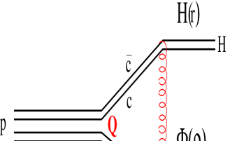
Figure 2: The two-gluon exchange diagram for the Higgs exclusive production

As discussed above, we shall assume the presence in the proton of an intrinsic charm (IC) component, a $\overline{c}c$ pair, which is predominantly in a color-octet state, and which has either a nonperturbative or perturbative origin. In the former case this heavy component can interact strongly with the $3q$ valence quark component. Such nonperturbative reinteractions of the intrinsic sea quarks in the proton wavefunction can lead to a $Q(x)\neq\overline{Q}(x)$ asymmetry as in the $\Lambda K$ model for the $s\overline{s}$ asymmetry [38, 39]. As in charmonium, the mean $\overline{c}c$ separation should be considerably larger than the transverse size $1/m_{c}$ of perturbative $\overline{c}c$ fluctuations. For instance, if the binding potential has the oscillator form, the mean distance is

$$\langle r_{\overline{c}c}^{2}\rangle=\frac{2}{\omega\,m_{c}}\ ,$$ (1)

where $\omega\sim 300\,\mbox{MeV}$ is the oscillation frequency. Alternatively, the IC component can be considered to derive perturbatively from the minimal gluonic couplings of the heavy quark pair to two valence quarks of the proton; this is likely the dominant mechanism at the largest values of $x_{c}$ [21]. In this case the transverse separation of the $\overline{c}c$ is controlled by the energy denominator, $\langle r_{\overline{c}c}^{2}\rangle=1/m_{c}^{2}$, and is much smaller than the estimate given by Eq. (1).

In accordance with the notation in Fig. 2 the two protons in the CM frame are detected with Feynman momentum fractions $x_{1}$ and $x_{2}$ and transverse momenta $\vec{p}_{1}$ and $\vec{p}_{2}$ respectively. Correspondingly, the produced Higgs carries longitudinal momentum $(x_{2}-x_{1})$ and transverse momentum $\vec{p}_{H}=-(\vec{p}_{1}+\vec{p}_{2})$. We assume the Higgs to be heavy, over $100\,\mbox{GeV}$, then $x_{1}$ and $x_{2}$ turn out to be tightly correlated in this reaction. Indeed, the effective mass squared of the $H-p_{1}$ pair reads,

$$M^{2}=\frac{M_{H}^{2}+\vec{p}_{H}^{\,2}}{1-x_{1}}+\frac{m_{p}^{2}+\vec{p}_{1}^{\,2}}{x_{1}}-\vec{p}_{2}^{\,2}\ .$$ (2)

(We assume the equivalence of Feynman $x$ and the corresponding fractions of the light-cone momenta, which is an accurate approximation at large $x$.) Due to the form factors of the two protons, neither transverse momenta, $\vec{p}_{1,2}$, can be much larger than a few hundred  MeV and therefore they, together with $\vec{p}_{H}$ and the proton mass, can be safely neglected in Eq. (2). This could be incorrect at very small values of $x_{1}\sim m_{p}^{2}/M_{H}^{2}$, but we will show that the $x_{1}$ distribution sharply peaks at $\overline{x}_{1}\approx 0.25$. Then, employing the standard relation $M^{2}/s=1-x_{2},$ we arrive at the simple relation,

$$(1-x_{1})(1-x_{2})=\frac{M_{H}^{2}}{s}\ .$$ (3)

The diffractive cross section has the form,

$$\frac{d\sigma(pp\to ppH)}{dx_{2}\,d^{2}p_{1}\,d^{2}p_{2}}=\frac{1}{(1-x_{2})16\pi^{2}}\left|A(x_{2},\vec{p}_{1},\vec{p}_{2})\right|^{2}\ ,$$ (4)

where the diffractive amplitude in Born approximation reads,

$$A(x_{2},\vec{p}_{1},\vec{p}_{2}) = \frac{8}{3\sqrt{2}}\,\int d^{2}Q\,\frac{d^{2}q}{q^{2}}\,\frac{d^{2}k}{k^{2}}\,\alpha_{s}(q^{2})\alpha_{s}(k^{2})\,\delta(\vec{q}+\vec{p}_{2}+\vec{k})\,\delta(\vec{k}-\vec{p}_{1}-\vec{Q})$$ (5)

$$\times \int d^{2}\tau\,\left|\Phi_{p}(\tau)\right|^{2}\left[e^{i(\vec{k}+\vec{q})\cdot\vec{\tau}/2}-e^{i(\vec{q}-\vec{k})\cdot\vec{\tau}/2}\right]\int d^{2}R\,d^{2}r\,d^{2}\rho\,H^{\dagger}(\vec{r})\ e^{i\vec{q}\cdot\vec{r}/2}$$

$$\times \left(1-e^{-i\vec{q}\cdot\vec{r}}\right)\Phi_{p}^{\dagger}(\vec{\rho})e^{i\vec{k}\cdot\vec{\rho}/2}\left(1-e^{-i\vec{k}\cdot\vec{\rho}}\right)\,\Psi_{p}(\vec{R},\vec{r},\vec{\rho},z)\,e^{i\vec{Q}\cdot\vec{R}}.$$

Here $\Psi_{p}(\vec{R},\vec{r},\vec{\rho},z)$ is the light-cone wave function of the IC component of the projectile proton with transverse separations $\vec{R}$ between the $\overline{c}c$ and $3q$ clusters, $\vec{r}$ between the $c$ and $\overline{c}$, $\vec{Q}$ is the relative transverse momentum of the $3q$ and $\overline{c}c$ clusters in the projectile and $\vec{\rho}$ is the transverse separation of the quark and diquark which couple to the final-state proton $p_{2}.$ The density $|\Phi_{p}(\tau)|^{2}$ is the wave function of the target proton which we also treat as a color dipole quark-diquark with transverse separation $\tau$. (The extension to three quarks is straightforward [37]). The fraction of the projectile proton light-cone momentum carried by the $\overline{c}c$, $z\approx 1-x_{1}$. This wave function is normalized as,

$$\int\limits_{0}^{1}dz\int d^{2}R\,d^{2}r\,d^{2}\rho\,\left|\Psi_{p}(\vec{R},\vec{r},\vec{\rho},z)\right|^{2}=P_{IC}\ ,$$ (6)

where $P_{IC}$ is the weight of the IC component of the proton, which is suppressed as $1/m_{c}^{2}$, and is assumed to be $P_{IC}\sim 1\%$. The amplitudes $H(\vec{r})$ and $\Phi_{p}(\vec{\rho})$ denote the wave functions of the produced Higgs and the outgoing proton, respectively, in accordance with Fig. 2.

The phase factors in Eq. (5) correspond to different attachments of the exchange gluons to quarks in Fig. 2. Thus, attaching the gluon either to the $c$, or to the $\overline{c}$ quarks one gets factor $[\exp(i\vec{q}\cdot\vec{r}/2)-\exp(-i\vec{q}\cdot\vec{r}/2)]$. An analogous factor corresponding to the second gluon coupling to the proton $p_{1}$ is also included in Eq. (5). The transverse coordinates of the quark and diquark in the target proton are $\tau/2$ and $-\tau/2$ (relative to its center of gravity). The phase factor in the square brackets in Ref. (5) thus includes two terms corresponding to attachment of the exchanged gluons to the same or different valence quark or diquark in $p_{2}$.

In order to advance the calculations further, we will take the following steps: First, we assume a factorized form of the proton wave function,

$$\Psi_{p}(\vec{R},\vec{r},\vec{\rho},z)=\Psi_{IC}(\vec{R},z)\,\Psi_{\overline{c}c}(\vec{r})\,\Psi_{3q}(\vec{\rho})\ .$$ (7)

Here $\Psi_{\overline{c}c}$ and $\Psi_{3q}$ are the $\overline{c}c$ and $3q$ wave functions normalized to unity, whereas $\Psi_{IC}(\vec{R},z)$ is the wave function describing the relative motion of the $\overline{c}c$ and $3q$ clusters, where $z$ is the fraction of the longitudinal momentum carried by the $\overline{c}c$. This wave function is normalized as,

$$\int d^{2}R\,\left|\Psi_{IC}(\vec{R},z)\right|^{2}=P_{IC}(z)\ ,$$ (8)

where $P_{IC}(z)$ is the $z$-distribution of $\overline{c}c$, related to the $x_{1}$ distribution of the produced protons, since with a very high precision $z=1-x_{1}=M_{H}^{2}/s(1-x_{2})$ (unless $x_{1}$ is as small as $x_{1}\sim 2m_{p}/\sqrt{s}$).

We will perform the calculations in Eq. (5) only for forward diffraction, i.e. $p_{2}=0$, $\vec{q}=-\vec{k}$, and we assume for the Pomeron the typical Gaussian $t$-dependence ($t=-p_{2}^{2}$),

$$\frac{d\sigma}{d^{2}p_{1}\,d^{2}p_{2}}\propto e^{-B(s^{\prime})p_{2}^{2}}\ ,$$ (9)

so the $t$-integrated cross section then reads,

$$\frac{d\sigma}{d^{2}p_{1}\,dx_{2}}=\left.\frac{\pi}{B(s^{\prime})}\,\frac{d\sigma}{d^{2}p_{1}\,d^{2}p_{2}\,dx_{2}}\right|_{p_{2}=0}\ .$$ (10)

Here the slope $B(s^{\prime})\sim B_{0}+2\alpha_{I\!\!P}^{\prime}\,\ln(s^{\prime}/M^{2}_{0})$, where $B_{0}=4\,\mbox{GeV}^{-2}$, $\alpha_{I\!\!P}^{\prime}=0.25\,\mbox{GeV}^{-2}$, $s^{\prime}/M_{0}^{2}=s/M_{H}^{2}$ and $M_{0}=1\,\mbox{GeV}$.

The next step is to replace the two-gluon proton vertex, represented by the integral over $\vec{\tau}$ in Eq. (5), by the unintegrated gluon density, ${\cal F}(x,k^{2})=\partial G(x,k^{2})/\partial({\rm ln}k^{2})$, where $G(x,Q^{2})=x\,g(x,Q^{2})$. This preserves the infra-red stability of the cross section, since ${\cal F}$ vanishes at $k^{2}\to 0$. The phenomenological gluon density fitted to data includes by default all higher order corrections and supplies the cross section with an energy dependence important for extrapolation to very high energies. One can relate the unintegrated gluon distribution to the phenomenological dipole cross section fitted to data for $F_{2}(x,Q^{2})$ from HERA, as was done in Ref. [40],

$${\cal F}(x,k^{2})=\frac{3\,\sigma_{0}}{16\,\pi^{2}\,\alpha_{s}(k^{2})}\ k^{4}\,R_{0}^{2}(x)\,{\rm exp}\Bigl{[}-{1\over 4}\,R_{0}^{2}(x)\,k^{2}\Bigr{]}\ .$$ (11)

The problem is the extrapolation to the small virtualities $k^{2}$ typical for the process under consideration. The Bjorken variable is not a proper variable for soft reactions; therefore we use the parametrization from Ref. [32] adjusted to data for soft interactions. Then $R_{0}(x)$ in Eq. (11) should be replaced by $R_{0}(s^{\prime})=0.88\,\,\mbox{fm}\times(s^{\prime}/s_{0})^{-\lambda/2}$ with $\lambda=0.28,$ $s_{0}=1000~{}\mbox{GeV}^{2}$ and $\sigma_{0}\Rightarrow\sigma_{0}(s^{\prime})=\sigma^{\pi p}_{tot}(s^{\prime})\,[1+3R^{2}_{0}(s^{\prime})/8\langle r^{2}_{ch}\rangle_{\pi}]$, where $\sigma^{\pi p}_{tot}(s^{\prime})=23.6\,\mbox{mb}\times(s^{\prime}/s_{0})^{0.08}$ is the Pomeron part of the $\pi p$ total cross section. The energy variable $s^{\prime}$ is related to the rapidity gap between the two protons in the final state, controlled by $x_{2}$,

$$s^{\prime}=\frac{M_{0}^{2}}{1-x_{2}}=s\,(1-x_{1})\,\frac{M_{0}^{2}}{M_{H}^{2}}\ .$$ (12)

Finally, combining all the above modifications and performing the $p_{1}$-integration in Eq. (5), we arrive at,

$$\frac{d\sigma^{IC}(pp\to ppH)}{dx_{2}} = \frac{32\pi\,P_{IC}(z)}{9\,B(s^{\prime})(1-x_{2})}\left|\int\frac{d^{2}k}{k^{4}}\,\alpha_{s}(k^{2})\,{\cal F}(x,k^{2})\,\right.$$ (13)

$$\times \left.\int d^{2}rH^{\dagger}(\vec{r})e^{-i\vec{k}\cdot\vec{r}/2}\left(1-e^{i\vec{k}\cdot\vec{r}}\right)\,\Psi_{\overline{c}c}(\vec{r})\right.$$

$$\times \left.\int d^{2}\rho\,\Phi_{p}^{\dagger}(\vec{\rho})e^{-i\vec{k}\cdot\vec{\rho}/2}\left(1-e^{i\vec{k}\cdot\vec{\rho}}\right)\,\Psi_{3q}(\vec{\rho})\right|^{2}\ .$$

Here

$$z=[x^{H}_{F}+\sqrt{(x_{F}^{H})^{2}+4M_{H}^{2}/s}]/2\approx x_{F}^{H}\approx 1-x_{1}=M_{H}^{2}/s(1-x_{2})\ .$$ (14)

This relation receives sizeable corrections only at very small Higgs Feynman $x^{H}_{F}\sim 2M_{H}/\sqrt{s}$. Notice that the expansion of the exponentials in Eq. (13) contains only odd powers of $\vec{k}\cdot\vec{r}$ and $\vec{k}\cdot\vec{\rho}$. This signals a change of orbital momentum of the quark configurations participating in the one-gluon exchange process. In order to obtain a nonzero result of the integration over $\vec{r}$, either the initial or the final $\overline{c}c$ wave function must contain a factor $\vec{\nabla}_{r}$, i.e. it must be a $P$-wave. Since we assume that the Higgs is a scalar, its $\overline{c}c$ component must be in a $P$-wave state, while the primordial $\overline{c}c$ in the projectile IC state should be in an $S$-wave. This is vice versa for the proton $p_{1}$: the final $|3q\rangle$ system is in an $S$-wave, but $\Psi_{3q}(\vec{\rho})$ must be a $P$-wave.

Notice that both the scalar Higgs and $\chi$ states may be produced from the same IC component of the proton containing $S$-wave $\overline{c}c$. However, the production of $J/\psi$, $\Upsilon$, $Z^{0}$ requires an IC component containing a $P$-wave $\overline{c}c$, which is presumably more suppressed.

The $P$-wave LC wave function of Higgs in impact parameter representation is given by the Fourier transform of its Breit-Wigner propagator:

$$H(\vec{r})=i\,\frac{\sqrt{N_{c}\,G_{F}}}{2\pi}\,m_{c}\,\overline{\chi}\,\vec{\sigma}\,\chi\,\frac{\vec{r}}{r}\,\left[\epsilon\,Y_{1}(\epsilon r)-{ir\over 2}\,\Gamma_{H}M_{H}\,Y_{0}(\epsilon r)\right]\ .$$ (15)

Here $G_{F}$ is the Fermi constant, $\chi$ and $\overline{\chi}$ are the spinors for $c$ and $\overline{c}$ respectively and

$$\epsilon^{2}=\alpha(1-\alpha)M_{H}^{2}-m_{c}^{2}\ ,$$ (16)

where $\alpha$ is the fraction of the LC momentum of the Higgs carried by the $c$-quark. The functions $Y_{0,1}(x)$ in Eq. (15) are the second order Bessel functions and $\Gamma_{H}$ is the total width of the Higgs. Assuming $\Gamma_{G}\ll M_{H}$, we neglect the second term in Eq. (15).

The LC wave function Eq. (16) assumes that the Higgs mass is much larger than the quark masses, which is probably true for charm and bottom. However, it is quite probable that for top-antitop in the Higgs $2m_{t}>M_{H}$, then the wave function is different,

$$H_{\overline{t}t}(\vec{r})=\frac{\sqrt{N_{c}\,G_{F}}}{2\pi}\,m_{t}\,\overline{\chi}\,\vec{\sigma}\,\chi\,\frac{\vec{r}}{r}\,\epsilon_{t}\,K_{1}(\epsilon_{t}r)\ ,$$ (17)

where $K_{1}(x)$ is the modified Bessel function and

$$\epsilon_{t}^{2}=m_{t}^{2}-\alpha(1-\alpha)M_{H}^{2}~{}~{}.$$ (18)

The probabilities computed from the wave functions Eqs. (15) and (18) require regularization in the ultraviolet limit [41, 42], as is the case of the $\overline{q}q$ wave function of a transverse photon. Such wave functions are not solutions of the Schrödinger equation, but are distribution functions for perturbative fluctuations. They are overwhelmed by very heavy fluctuations with large intrinsic transverse momenta, or vanishing transverse separations. Such point-like fluctuations lead to a divergent normalization, but they do not interact with external color fields, i.e.they are not observable. All the expressions for any measurable quantity, including the cross section, are finite.

As we have discussed, the IC wave function can be modeled as a nonperturbative $5-quark$ stationary state $|3qc\overline{c}\rangle$, or as a perturbative fluctuation $|3q\rangle\to|3qc\overline{c}\rangle$. Correspondingly, the $\overline{c}c$ wave function within the Fock state will be assumed to be a linear combination of nonperturbative and perturbative distribution amplitudes,

$$\Psi_{\overline{c}c}(\vec{r})=\beta\,\Psi^{npt}_{\overline{c}c}(\vec{r})+\sqrt{1-\beta^{2}}\,\Psi^{pt}_{\overline{c}c}(\vec{r})\ .$$ (19)

The parameter $\beta$ which controls the relation between the nonperturbative and perturbative IC contributions, is such that $0\leq\beta\leq 1$. The nonperturbative wave function should be an S-wave solution of the Schrödinger equation. Assuming oscillator potential we get,

$$\Psi^{npt}_{\overline{c}c}(\vec{r})=\sqrt{\frac{m_{c}\omega}{2\pi}}\,\exp(-r^{2}\,m_{c}\,\omega/4)\ ,$$ (20)

where $\omega$ is the oscillation frequency, as mentioned earlier.

Since the Higgs is produced from an $S$-wave $\overline{c}c$, the perturbative distribution amplitude is ultraviolet stable and can be normalized to one, in order to correspond to $P_{c}$ as a probability to have such a charm quark pair in the proton

$$\Psi^{pt}_{\overline{c}c}(\vec{r})=\frac{m_{c}}{\sqrt{\pi}}\,K_{0}(m_{c}r)\ .$$ (21)

Here the modified Bessel function $K_{0}(m_{c}r)$ is the Fourier transform of the energy denominator associated with the $\overline{c}c$ fluctuation. We assume the $c$ and $\overline{c}$ quarks to carry equal fractional momenta. For fixed $\alpha_{s}$ the energy denominator governs the probability of the fluctuation in momentum space, since perturbatively one treats the charm quarks as free particles.

Now we can calculate the part of the matrix element in Eq. (13) related to Higgs production from the IC. We assume the initial $\overline{c}c$ wave function to be a linear combination (19) of the nonperturbative, Eq. (20) and perturbative, Eq. (21) wave functions, and the final state wave function of the $\overline{c}c$ pair in the Higgs in the form (15). The result reads,

$$\int d^{2}r\,H^{\dagger}(\vec{r})\,e^{i\vec{k}\cdot\vec{r}/2}\left(1-e^{-i\vec{k}\cdot\vec{r}}\right)\Psi_{\overline{c}c}(\vec{r})=\frac{4}{\sqrt{\pi}}\,\frac{m_{c}^{2}}{M_{H}^{2}}\sqrt{N_{c}G_{F}}\ \overline{\chi}\,\vec{\sigma}\,\chi\,\vec{k}$$ (22)

$$\times \left[\beta\,\sqrt{\frac{\omega}{2m_{c}}}+\sqrt{1-\beta^{2}}\,\ln\left(\frac{M_{H}}{2m_{c}}\right)\right]\ .$$

Here we have made use of $M_{H}\gg m_{c}$ and expanded the exponentials $\exp(\pm i\vec{k}\cdot\vec{r})$ up to the first nonvanishing term. We also dropped the integration over $\alpha$, assuming that the $c$ and $\overline{c}$ in the IC component carry the same momentum, i.e. $\Psi_{\overline{c}c}(r,\alpha)=\Psi_{\overline{c}c}(r)\,\delta(\alpha-1/2)$. Correspondingly, we have fixed $\epsilon=M_{H}/2$ and we will assume $\beta\ll 1$.

The result of integration in Eq. (22) shows that the perturbative contribution is quite enhanced relative to the nonperturbative term. First of all, the enhancement by factor $\sqrt{2m_{c}/\omega}$ is due to the fact that the projection to the point-like Higgs wave function is proportional to $\Psi_{\overline{c}c}^{IC}(0)$, and the perturbative fluctuation has a smaller radius. Another enhancement factor, $\ln(M_{H}/2m_{c})$, is due to the long power tail in the momentum distribution in the perturbative IC wave function, which the nonperturbative one has a Gaussian cut off. Thus, the perturbative term in the matrix element Eq. (22) is relatively enhanced by one order of magnitude.

Notice that the nonrelativistic nonperturbative solution should not be used for convolution with the highly perturbative Higgs wave function. The large transverse momentum tail of the IC should be represented by the perturbative term in Eq. (19). Unfortunately, the normalization of such a perturbative tail is unknown, and we normalize it to the IC weight $1\%$.

Enhancement of the perturbative intrinsic heavy flavor in Higgs production is especially large for the top component. Using the IT wave function Eq. (17) we get

$$\int d^{2}r\,H_{\overline{t}t}^{\dagger}(\vec{r})\,e^{i\vec{k}\cdot\vec{r}/2}\left(1-e^{-i\vec{k}\cdot\vec{r}}\right)\Psi^{pt}_{\overline{t}t}(\vec{r}) = \frac{1}{\sqrt{\pi}}\,\frac{m_{t}^{2}}{M_{H}^{2}}\sqrt{N_{c}G_{F}}\ \overline{\chi}\,\vec{\sigma}\,\chi\,\vec{k}$$ (23)

$$\times \left[1+\frac{1-\delta}{\delta}\,\ln(1-\delta)\right]\ ,$$

where $\delta=M_{H}^{2}/4m_{t}^{2}$.

The proton is produced in a similar way from the P-wave $3q$ in the projectile IC component. The exponentials, however, should not be expanded, since the radius is not small. Therefore, using the relation,

$$\int\limits_{0}^{2\pi}d\phi\,\vec{\rho}\,\left(e^{i\vec{\rho}\cdot\vec{k}/2}-e^{-i\vec{\rho}\cdot\vec{k}/2}\right)=4\pi i\,\rho\,\frac{\vec{k}}{k}\,J_{1}(k\rho/2)\ ,$$ (24)

we get for the integral over $d^{2}\rho$ in Eq. (13),

$$\int d^{2}\rho\,\frac{1}{\sqrt{\pi}R_{3q}}\,\frac{\vec{\rho}}{\rho}\,e^{-\rho^{2}/2R_{3q}^{2}}\left(e^{i\vec{\rho}\cdot\vec{k}/2}-e^{-i\vec{\rho}\cdot\vec{k}/2}\right)\frac{1}{\sqrt{\pi}R_{p}}\,e^{-\rho^{2}/2R_{p}^{2}}$$ (25)

$$= i\,\frac{\sqrt{\pi}}{4}\,\frac{{\cal R}^{3}\,\vec{k}}{R_{p}\,R_{3q}}\,e^{-y}\left[J_{0}(y)-J_{1}(y)\right]\ ,$$

where ${\cal R}^{2}=2\,R_{p}^{2}\,R_{3q}^{2}/(R_{p}^{2}+R_{3q}^{2})$, and $y={\cal R}^{2}\,k^{2}/32$. For further estimates we assume that $R_{p}=R_{3q}$, so ${\cal R}=R_{p}$. Since we assumed a meson-type quark-diquark structure for the proton, the mean separation $R_{p}^{2}=2\langle r_{ch}^{2}\rangle_{p}/3$. The transition proton form factor, $\exp(-k^{2}{\cal R}^{2}/32)$, cuts off the integration over $d^{2}k$.

Now we are in a position to perform the last integration over $\vec{k}$ in Eq. (13),

$$\frac{d\sigma^{IC}(pp\to ppH)}{dx_{2}}=\frac{32}{\pi^{2}}\,\frac{G_{F}\,P_{IC}(z)}{1-x_{2}}\,\frac{m_{c}^{4}}{M_{H}^{4}}\,\frac{[\sigma^{\pi p}_{tot}(s^{\prime})]^{2}}{B(s^{\prime})\,\langle r^{2}_{ch}\rangle_{p}}\,\frac{\gamma^{2}(s^{\prime})}{[2+2\gamma(s^{\prime})+\gamma^{2}(s^{\prime})]^{3}}$$ (26)

$$\times \left[1+\frac{\langle r^{2}_{ch}\rangle_{p}}{16\,\langle r^{2}_{ch}\rangle_{\pi}}\,{1\over\gamma(s^{\prime})}\right]^{2}\,\left[\beta\,\sqrt{\frac{\omega}{2m_{c}}}+\sqrt{1-\beta^{2}}\,\ln\left(\frac{M_{H}}{2m_{c}}\right)\right]^{2}\ ,$$

where $\gamma(s^{\prime})=R_{p}^{2}/4R_{0}^{2}(s^{\prime})$.

The cross section of Higgs production from the intrinsic bottom has the same form as Eq. (26), and we assume that the weight of intrinsic heavy flavor scales as, $P_{IQ}=P_{IC}m_{c}^{2}/m_{Q}^{2}$. However, as we found above, if the Higgs mass is restricted by $M_{H}^{2}<4m_{t}^{2}$, production from intrinsic perturbative top component of the proton has cross section,

$$\frac{d\sigma^{IT}(pp\to ppH)}{dx_{2}}=\frac{8}{\pi^{2}}\,\frac{G_{F}\,P_{IT}(z)}{1-x_{2}}\,\frac{m_{t}^{4}}{M_{H}^{4}}\,\frac{[\sigma^{\pi p}_{tot}(s^{\prime})]^{2}}{B(s^{\prime})\,\langle r^{2}_{ch}\rangle_{p}}\,\frac{\gamma^{2}(s^{\prime})}{[2+2\gamma(s^{\prime})+\gamma^{2}(s^{\prime})]^{3}}$$ (27)

$$\times \left[1+\frac{\langle r^{2}_{ch}\rangle_{p}}{16\,\langle r^{2}_{ch}\rangle_{\pi}}\,{1\over\gamma(s^{\prime})}\right]^{2}\,\left[1+\frac{1-\delta}{\delta}\,\ln(1-\delta)\right]^{2}\ .$$

4.2 Feynman $x^{H}_{F}$ distribution of Higgs particles

The $x_{F}^{H}$ distribution of the cross section Eqs. (26)-(27) is related to the LC wave function $\Psi_{IC}(R,z)$ of the system $3q-\overline{c}c$, namely to the function $P_{IC}(z)$ defined in Eq. (8). The momentum fraction $z$ is related to $x_{1,2}$ and $x_{F}^{H}$ by Eq. (14). The shape of $P_{IC}(z)$ strongly correlates with the origin of IC, a nonperturbative component of the proton wave function or a perturbative fluctuation.

4.2.1 Nonperturbative IC

In principle one can construct hadronic LC wave function by diagonalizing the LC Hamiltonian. Here we will use the method of Ref. [43] for the Lorentz boost of the wave function, which is supposed to be known in the hadron rest frame. The Lorentz boost generates higher particle number quantum fluctuations which are missed by this procedure; however this method works well in known cases  [44, 45], and even provides a nice cancelation of large terms violating the Landau-Yang theorem  [46].

We assume that the rest frame IC wave function has the oscillatory form (in momentum space),

$$\tilde{\Psi}_{IC}(\vec{Q},z)=\sqrt{P_{IC}(z)}\left(\frac{1}{\pi\omega\mu}\right)^{3/4}\exp\left(-\frac{\vec{Q}^{2}}{2\omega\mu}\right)\ .$$ (28)

Here $\omega$ stands for the oscillator frequency and $\mu=M_{\overline{c}c}M_{3q}/(M_{\overline{c}c}+M_{3q})$ is the reduced mass of the $\overline{c}c$ and $3q$ clusters. For further estimates we use $M_{\overline{c}c}=3\,\mbox{GeV}$ and $M_{3q}=1\,\mbox{GeV}$, although the latter could be heavier, since it is the $P$-wave.

To express the 3-vector $\vec{Q}$ by the effective mass of the system, $M_{eff}=\sqrt{\vec{Q}^{2}+M_{\overline{c}c}^{2}}+\sqrt{\vec{Q}^{2}+M_{3q}^{2}}$, one can switch to the LC variables, $\vec{Q}$ and $z$,

$$M_{eff}^{2}=\frac{Q^{2}}{z(1-z)}+\frac{M_{\overline{c}c}^{2}}{z}+\frac{M_{3q}^{2}}{1-z}\ .$$ (29)

Then the longitudinal component $Q_{L}$ in the exponent in (28) reads,

$$Q_{L}^{2}=\frac{M_{eff}^{2}}{4}+\frac{(M_{\overline{c}c}^{2}-M_{3q}^{2})^{2}}{4M_{eff}^{2}}-\frac{M_{\overline{c}c}^{2}+M_{3q}^{2}}{2}-Q^{2}\ ,$$ (30)

and the LC wave function acquires the form,

$$\Psi_{IC}(Q,z)=K\,\sqrt{P_{IC}(z)}\,\exp\left\{-\frac{1}{8\omega\mu}\left[M_{eff}^{2}+\frac{(M_{\overline{c}c}^{2}-M_{3q}^{2})^{2}}{M_{eff}^{2}}\right]\right\}\ ,$$ (31)

where

$$K^{2} = \frac{1}{8Q_{L}}\,\left(\frac{1}{\pi\omega\mu}\right)^{3/2}\,\exp\left(\frac{M_{\overline{c}c}^{2}+M_{3q}^{2}}{2\omega\mu}\right)\,\left[1-\frac{(M_{\overline{c}c}^{2}-M_{3q}^{2}}{M_{eff}^{4}}\right]$$ (32)

$$\times \left[\frac{Q^{2}(2z-1)}{z^{2}(1-z)^{2}}-\frac{M_{\overline{c}c}^{2}}{z^{2}}+\frac{M_{3q}^{2}}{(1-z)^{2}}\right]~{}.$$

Now we can calculate the $z$-dependence of the function $P_{IC}(z)$ defined in Eq. (8), which controls the $x_{1}$ dependence of the cross section,

$$\frac{P_{IC}(z)}{P_{IC}}=\ \frac{1}{\sigma^{IC}(pp\to ppH)}\,\frac{d\sigma^{IC}(pp\to ppH)}{dx_{1}}=\frac{1}{P_{IC}}\int d^{2}Q\,\left|\Psi_{IC}(Q,z)\right|^{2}~{}.$$ (33)

This function is plotted in Fig. 3.

Figure 3: The distribution of produced Higgs particles over the fraction of the proton beam momentum. The dotted, dashed and solid curves correspond to Higgs production from nonperturbative IC ($\beta=1$), perturbative IC ($\beta=0$) and IT, respectively.

The distribution sharply picks at $z\approx 0.75$, as one could expect, since the IC pair is heavy and should carry the main fraction of the proton momentum. Note that at high energies, in particular at LHC, the momentum fraction $z$ coincides with the Feynman $x_{H}$ of the Higgs particle, with a high accuracy $\sim M_{H}^{2}/s$.

4.2.2 Perturbative intrinsic heavy flavors

The light-cone wave function of a perturbative fluctuation $p\to|3q\overline{Q}Q\rangle$ in momentum representation is controlled by the energy denominator,

$$\Psi_{IQ}(Q,z,\kappa)\propto\frac{z(1-z)}{Q^{2}+z^{2}m_{p}^{2}+M^{2}_{\overline{Q}Q}(1-z)}\ .$$ (34)

Momentum $\vec{Q}$ was defined in Fig. 2 and Eq. (5). The effective mass of the $\overline{Q}Q$ depends on the intrinsic transverse momentum of the $\overline{Q}Q$ pair, $M_{\overline{Q}Q}^{2}=4(\kappa^{2}+m_{Q}^{2})$. It is controlled by the convolution of the IC $\overline{Q}Q$ wave function with the $P$-wave $\overline{Q}Q$ wave function in the Higgs and the one-gluon exchange amplitude (see Fig. 2), which has the form,

$$\int\limits_{0}^{\infty}d\kappa^{2}\,\Psi_{IQ}(Q,z,\kappa)\left[H_{\overline{Q}Q}(\vec{\kappa}+\vec{k}/2)-H_{\overline{Q}Q}(\vec{\kappa}-\vec{k}/2)\right]$$ (35)

$$\propto z(1-z)\,\frac{\ln\left[\frac{\left|M_{H}^{2}-4m_{Q}^{2}\right|(1-z)}{Q^{2}+4m_{Q}^{2}(1-z)+m_{p}^{2}z^{2}}\right]}{M_{H}^{2}(1-z)+Q^{2}+m_{p}^{2}z^{2}}\ .$$

This expression peaks at $1-z\sim m_{p}/M_{H}$, therefore the logarithmic factor hardly varies as function of $Q^{2}$ which is restricted by the proton form factor. Making use of this we perform integration in Eq. (33) and arrive at the following $z$-distribution,

$$\frac{P_{IQ}(z)}{P_{IQ}}=Nz(1-z)\,\frac{\left\{\ln\left[\frac{\left|M_{H}^{2}-4m_{Q}^{2}\right|(1-z)}{4m_{Q}^{2}(1-z)+m_{p}^{2}z^{2}}\right]\right\}^{2}}{M_{H}^{2}(1-z)+m_{p}^{2}z^{2}}\ ,$$ (36)

where $N$ is a constant normalizing to one the integral over $z$. The corresponding $z$-distributions for charm and top are shown in Fig. 3 by dotted (dashed) and solid curves respectively.

4.3 Energy dependence

One can integrate in Eqs. (26)-(27) over $x_{2}$ using relation (14). Since the momentum distribution of Higgs produced from the nonperturbative IC sharply peaks at $z=z_{0}=0.75$, one can replace $P_{IC}(z)\Rightarrow\delta(z-z_{0})\,P_{IC}$. With a reasonable accuracy we can fix $z$ at the same value for the perturbative case and heavier flavors too, which is justified by the rather mild dependence on $\tilde{s}$ of other factors in Eqs. (26)-(27).

Since at high energies $z\approx x_{H}\approx 1-x_{1}$, performing integration in Eq. (26) one arrives at,

$$\sigma^{IC}(pp\to ppH)=\frac{32}{\pi^{2}}\,\frac{G_{F}\,P_{IC}}{z_{0}}\,\frac{m_{c}^{4}}{M_{H}^{4}}\,\frac{[\sigma^{\pi p}_{tot}(\tilde{s})]^{2}}{B(\tilde{s})\,\langle r^{2}_{ch}\rangle_{p}}\,\frac{\gamma^{2}(\tilde{s})}{[2+2\gamma(\tilde{s})+\gamma^{2}(\tilde{s})]^{3}}$$ (37)

$$\times \left[1+\frac{\langle r^{2}_{ch}\rangle_{p}}{16\,\langle r^{2}_{ch}\rangle_{\pi}}\,{1\over\gamma(\tilde{s})}\right]^{2}\,\left[\beta\,\sqrt{\frac{\omega}{2m_{c}}}+\sqrt{(1-\beta^{2})}\,\ln\left(\frac{M_{H}}{2m_{c}}\right)\right]^{2}\ ,$$

where $\tilde{s}=s\,z_{0}\,M_{0}^{2}/M_{H}^{2}$. Analogous expression should be valid for Higgs production from intrinsic bottom. For top quark in the proton we use Eq. (27) which leads to,

$$\sigma^{IT}(pp\to ppH)=\frac{8}{\pi^{2}}\,\frac{G_{F}\,P_{IT}}{z_{0}}\,\frac{m_{t}^{4}}{M_{H}^{4}}\,\frac{[\sigma^{\pi p}_{tot}(\tilde{s})]^{2}}{B(\tilde{s})\,\langle r^{2}_{ch}\rangle_{p}}\,\frac{\gamma^{2}(\tilde{s})}{[2+2\gamma(\tilde{s})+\gamma^{2}(\tilde{s})]^{3}}$$ (38)

$$\times \left[1+\frac{\langle r^{2}_{ch}\rangle_{p}}{16\,\langle r^{2}_{ch}\rangle_{\pi}}\,{1\over\gamma(\tilde{s})}\right]^{2}\,\left[1+\frac{1-\delta}{\delta}\,\ln(1-\delta)\right]^{2}\ .$$

Notice that function $\gamma(\tilde{s})$ increases with energy as $s^{0.28}$, and such a steep rise of the denominator in Eq. (37) is not compensated by the rise of the total cross section in the numerator. Therefore, the diffractive cross sections, Eqs. (37)-(38), turns out to decrease at asymptotic energies approximately as inverse energy. This unexpected result may be interpreted as follows. The source of the falling energy dependence is the steep rise with energy of the mean transverse momentum of gluons as is given by the unintegrated gluon density Eq. (11), $\langle k^{2}\rangle=4/R_{0}^{2}(x)\propto(s/M_{H}^{2})^{0.28}$. Also the integral over $k^{2}$ of the distribution (11) rises with energy, and its value at $k=0$ is steeply falling. The rise comes for large transverse momenta which, however, are cut off by the nucleon form factor Eq. (20). This is why the diffractive cross section (37) is steeply falling. Indeed, without this form factor, for instance in the reaction $pp\to HXp$, the cross section would rise as $(s/M_{H})^{0.7}$.

Nevertheless, at the energy of LHC, $\sqrt{s}=14\,\mbox{TeV}$, the effective energy is rather low, $\sqrt{\epsilon}s=120\,\mbox{GeV}$ (we assume $M_{H}=100\,\mbox{GeV}$) the cross section still rises with energy. Indeed, $R_{0}^{2}=0.36\,\mbox{fm}^{2}$, so $\gamma(\epsilon s)=0.55$ is still rather small at this energy, and the cross sections Eqs. (37)-(38) rise as,

$$\sigma^{IQ}(pp\to ppH)_{LHC}\propto\left(\frac{s}{M_{H}^{2}}\right)^{0.6}\ .$$ (39)

However, at much higher energies the energy dependence will switch to a steeply falling one. Besides, absorptive or unitarity corrections are known to slow down the rise of the cross sections.

4.4 Absorptive corrections

The amplitude of any off-diagonal large rapidity gap process is subject to unitarity or absorptive corrections, which have the intuitive meaning of a survival probability of the participating hadrons. To include these corrections one should replace the diffractive amplitude as,

$$f^{pp}_{sd}(b,s)\Rightarrow f^{pp}_{sd}(b,s)\,\left[1-\,\mbox{Im}\,f^{pp}_{el}(b,s)\right]\ ,$$ (40)

The data for elastic $pp$ scattering show that the partial amplitude $f^{pp}_{el}(b,s)$ is constant energy at small impact parameters $b\to 0$, while rising as function of energy at large $b$ [47, 48, 49]. This is usually interpreted as a manifestation of saturation of the unitarity limit, $\,\mbox{Im}\,f^{pp}_{el}\leq 1$. Indeed, this condition imposes a tight restriction at small $b$, where $\,\mbox{Im}\,f^{pp}_{el}\approx 1$, leaving almost no room for further rise. We will treat the Pomeron as a Regge pole without unitarity corrections:

$$\,\mbox{Im}\,f^{pp}_{el}(b,s)=\frac{\sigma^{pp}_{tot}(s)}{4\pi B^{pp}_{el}(s)}\ \exp\left[-\frac{b^{2}}{2B^{pp}_{el}(s)}\right]\ ,$$ (41)

where $\sigma^{pp}_{tot}(s)=21.8\,\mbox{mb}\times(s/M_{0}^{2})^{\epsilon}$, and $\epsilon=0.08$; $B^{pp}_{el}(s)=B^{0}_{el}+2\,\alpha^{\prime}_{{I\!\!P}}\,\ln(s/M_{0}^{2})$ with $B^{0}_{el}=7.5\,\mbox{GeV}^{-2}$. Due to the accidental closeness of $2\alpha_{{I\!\!P}}^{\prime}/B^{0}_{el}=0.067$ and $\epsilon$, the pre-exponential factor in (41) hardly changes with energy even without unitarity corrections. It is demonstrated in Ref. [49] that not only at $b=0$, but in the whole range of impact parameters, the model Eq. (41) describes correctly the energy dependence of the partial amplitude $f^{pp}_{el}(b,s)$.

Thus we arrive at the absorption corrected cross section,

$$\tilde{\sigma}^{IQ}(pp\to ppH)=\sigma^{IQ}(pp\to ppH)\,$$ (42)

$$\times \left\{1-{1\over{\pi}}\,\frac{\sigma^{pp}_{tot}(s^{\prime})}{B(s^{\prime})+2B^{pp}_{el}(s^{\prime})}+\frac{1}{(4\pi)^{2}}\,\frac{\left[\sigma^{pp}_{tot}(s^{\prime})\right]^{2}}{B^{pp}_{el}(s^{\prime})\left[B(s^{\prime})+B^{pp}_{el}(s^{\prime})\right]}\right\}\ .$$

This is not a severe suppression even at the energy of LHC, where the absorptive factor is $0.2$.

Including the absorptive corrections we calculated the total cross sections for diffractive Higgs production, $pp\to Hpp$, from the IQ components. The results at the energy of LHC, $\sqrt{s}=14\,\mbox{TeV}$, are plotted as function of Higgs mass in the Fig. 4. We assume a perturbative origin for all intrinsic components, a $1/m_{Q}^{2}$ scaling for their weights, and $1\%$ probability of IC for $\beta=0$ in Eq. (37).

Figure 4: The cross section of the reaction $pp\to Hp+p$ as function of the Higgs mass. Contributions of IC (dashed) of IB (dotted) and IT (solid).

Note that the contributions of the intrinsic charm and bottom falls steeply with the mass of the Higgs in accordance with Eq. (37). The contribution of the intrinsic top rises with $M_{H}$ unless $M_{H}>2m_{t}\approx 350\,\mbox{GeV}$, then the cross section starts falling.

5 Further possibilities to get a larger cross section

5.1 Direct production of Higgs from a colorless IQ

A heavy flavor $\overline{Q}Q$ pair in the IQ component of the proton may be found in a colorless state. In this case the Higgs particle can be produced directly from this pair via Pomeron exchange as is shown in Fig. 5.

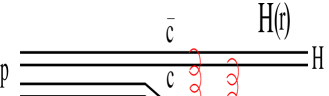
Figure 5: Higgs production via Pomeron exchange

We consider the example of intrinsic charm of a nonperturbative origin throughout this section.

At first glance one may think that this channel is less suppressed by powers of the Higgs mass compared to the mechanism presented in Fig. 2. Indeed, the integration over $\vec{k}$ does not have the upper cutoff imposed by the proton form factor in the previous case; therefore it may compensate two powers of $M_{H}$ in the amplitude. This analysis is correct. Nevertheless the amplitude turns out to be more suppressed than in the diagram Fig. 2.

The diffractive amplitude $A(x_{2},\vec{p}_{1},\vec{p}_{2})$ is proportional to the matrix element of the dipole cross section $\sigma_{\overline{q}q}(r)$ between the initial $\overline{c}c$ wave function $\Psi_{\overline{c}c}(r)$ and the distribution amplitude of the $\overline{c}c$ in the Higgs,

$$A(x_{2},\vec{p}_{1},\vec{p}_{2})\propto\int d^{2}r\,H^{\dagger}(\vec{r})\,\sigma_{\overline{q}q}(r)\,\Psi_{\overline{c}c}(r)\ .$$ (43)

This factor contains all the dependence on the Higgs mass. To estimate it one can use a Gaussian shape for both $\Psi_{\overline{c}c}(r)$ and $H(\vec{r})$. Then one finds $A\propto\sqrt{m_{c}\omega}/M_{H}^{3}$. A more refined calculation confirms this,

$$\int d^{2}r\,H^{\dagger}(\vec{r})\,\sigma_{\overline{q}q}(r)\,\Psi_{\overline{c}c}(r) = \frac{3\sigma_{0}(s)\sqrt{2\pi N_{c}G_{F}}}{2m_{c}\omega\,R_{0}^{2}(s)}\ {\rm U}\left({3\over 2},0,\frac{M_{H}^{2}}{4m_{c}\omega}\right)$$ (44)

$$= \frac{12\sigma_{0}(s)}{R_{0}^{2}(s)}\,\sqrt{2\pi N_{c}G_{F}}\,\frac{\sqrt{m_{c}\omega}}{M_{H}^{3}}\ ,$$

where the initial state $\overline{c}c$ pair is assumed to be in a $P$-wave. Here $U(a,b,x)$ is the confluent hypergeometric function, and we use its asymptotic behavior at $x\gg 1$,

$$U(a,b,x)=x^{-a}+O(x^{-a-1})\ .$$ (45)

Notice that a convolution similar to Eq. (43) also defines the scale dependence of the amplitude of photoproduction of heavy quarkonia, which also behaves like $(Q^{2}+M^{2})^{-3}$. Thus, the complementary mechanism of diffractive Higgs production, besides the smaller probability to find the colorless IC component, is additionally suppressed by $1/M_{H}^{2}$ compared to the dominant mechanism depicted in Fig. 2. Therefore, this contribution can be safely neglected.

5.2 Nuclear enhancement

The produced Higgs is supposed to escape detection and to be identified only by using the missing mass spectrum. One may also consider the same reaction on a bound proton in $pA$ collisions where the nuclear debris spectators flying in the same direction as the Higgs. The nuclear enhancement in this case is not as large as one could naively expect. The reason is that absorptive corrections are stronger than those considered above in Sect. 4.4 for the case of $pp$ collisions. The survival probability represented by the last factor in Eq. (42) can be evaluated within the Glauber approximation for $pA$ collisions as

$$Z_{eff}=\frac{Z}{A}\int d^{2}b\,T_{A}(b)\,e^{-\sigma^{pp}_{in}T_{A}(b)}\ ,$$ (46)

where $T_{A}(b)=\int_{-\infty}^{\infty}dz\,\rho_{A}(b,z)$ is the nuclear thickness function at impact parameter $\vec{b}$, and $\rho_{A}(b)$ is the nuclear density. We assume here that diffractive recoil neutrons cannot be detected; otherwise the factor (46) should be multiplied by $A/Z$.

The nuclear enhancement for lead according to (46) is rather mild, of about an order of magnitude, since $Z_{eff}\approx 2.5$ should be compared with the suppression factor $0.2$, for $pp$ collisions calculated in Sect. 4.4. Gribov corrections [50] are known to make nuclei more transparent, therefore they may substantially increase the survival probability factor [51, 31]. If we employ the simplest quadratic dependence of the dipole cross section $\sigma_{\overline{q}q}(r)\propto r^{2},$ then the nuclear enhancement is considerably larger, a factor of about $50$.

6 Conclusions

The key assumption underlying our analysis of high $x_{F}$ Higgs hadroproduction is the presence of intrinsic heavy flavor $|uudQ\overline{Q}>$ Fock components in the proton bound-state wave function. Such quantum fluctuations are in fact rigorous consequences of QCD. The the probability for intrinsic heavy quark on the heavy quark mass falls as $\Lambda^{2}_{QCD}\over M_{Q}^{2}$ in non-abelian theories and can be computed from the operator product expansion  [11]. In such Fock states the heavy quarks $Q$ and $\overline{Q}$ carry the highest light-cone momentum fractions. Thus although they have small probability, intrinsic heavy quark Fock states are highly efficient in transferring the momentum of the proton to the momenta of particles in the final-state, especially heavy quarkonium and the Higgs which can sum the momenta of both the $Q$ and $\overline{Q}$. It is thus interesting and important that measurements of the production of heavy quarkonium at high $x_{F}$ as well as other heavy hadrons such as the $\Lambda_{b}$ and $\Lambda_{c}$ be carried out at RHIC, the Tevatron, as well as the LHC in order to test this novel feature of QCD.

As we have reviewed in section 3, there is substantial but not conclusive phenomenological evidence for intrinsic charm at the $1\%$ probability level in the proton. It is thus particularly important to have measurements of the charm and bottom structure functions in deep inelastic lepton-proton scattering over the full range of $x_{bJ}$. One must allow for intrinsic sea components at any scale $Q_{0}$ when parameterizing the proton’s structure functions, since the intrinsic Fock states are responsible for the $\overline{u}(x)\neq\overline{d}(x)$, $s(x)\neq\overline{s}(x)$ asymmetries, as well as the high-$x$ $c(x)$ and $b(x)$ distributions. There are also important nuclear and heavy quark threshold effects related to intrinsic charm which can be tested at lower energy fixed-target facilities such as JLAB, GSI-FAIR, and J-PARC [52].

As we have emphasized here, the materialization of intrinsic heavy flavor states in the proton leads to Higgs production in the proton fragmentation region: this includes inclusive production $pp\to HX,$ singly diffractive production $pp\to p+HX$ and exclusive diffractive production $pp\to p+H+p$, reactions which should be considered in addition to the conventional central rapidity production processes. The fractional momentum distribution for a Higgs produced by combining the momenta of both heavy quarks in the IQ Fock states is presented in Fig. 3. As seen in the figure, the Higgs can be produced with momentum fractions as large as $x_{F}\sim 0.8$ or even higher. One also produce the Higgs inclusively from leading-twist PQCD processes such as $gc\to Hc$ and $gb\to Hb$ where the high momentum of one intrinsic heavy quark is transferred to the Higgs.

We have focused in this paper on diffractive exclusive Higgs production $pp\to p+H+p,$ since in principle, only the final-state protons need to be measured and the Higgs can be reconstructed from the missing mass distribution. We note, however, that detecting the diffractive signal $pp\to p+H+p$ poses new challenges: When the Higgs is produced at large $x_{F}$, one of the final-state protons will be need to be detected at a small momentum fraction $\sim 1-x_{F}$, which is outside of the usual acceptance of forward proton detectors.

The underlying color structure of the intrinsic Fock state and the gauge theory properties of the two-gluon exchange mechanism for high energy diffraction play key roles in the physics of the exclusive diffractive Higgs hadroproduction process. The main result of our analysis, the cross sections given in Eqs. (37,38), demonstrates that the heavier the intrinsic heavy quark, the larger is the cross section for the doubly diffractive reaction. It rises with $m_{Q}$ linearly if the heavy quarks are confined by a potential, and is presented in Fig. 4 if the $\overline{Q}Q$ appear in the proton as a perturbative fluctuation. The production cross section also steeply rises with energy $\propto s^{0.7}$, which is characteristic for the energy dependence of hard reactions. Absorptive correction slow down this rise and eventually stop it at very high energies, above the energy range of LHC. Asymptotically, in the Froissart regime, this cross section is expected to fall. Numerical predictions for diffractive Higgs production from IC, IB and IT components are shown in Fig. 4. The cross section will be further enhanced from possible Fock states of the proton containing supersymmetric partners of quarks or gluons. We also have discussed a potential increase in the rate for such reactions using proton-nucleus collisions.

Acknowledgments: Work supported in part by the Department of Energy under contract number DE-AC02-76SF00515, by Fondecyt (Chile) grant numbers 1030355 and 1050519, by DFG (Germany) grant PI182/3-1 and by the cooperation program Ecos-Conicyt C04E04 between France and Chile.

We are thankful to Fred Goldhaber, Paul Hoyer and Alexander Tarasov for informative and helpful discussions.

References

- [1] S. J. Brodsky, C. Peterson and N. Sakai, Phys. Rev. D 23, 2745 (1981).
- [2] S. J. Brodsky, P. Hoyer, C. Peterson and N. Sakai, Phys. Lett. B 93, 451 (1980).
- [3] J. Pumplin, arXiv:hep-ph/0508184.
- [4] H. P. Nilles, Phys. Rept. 110, 1 (1984).
- [5] A. De Roeck, V. A. Khoze, A. D. Martin, R. Orava and M. G. Ryskin, Eur. Phys. J. C 25, 391 (2002) [arXiv:hep-ph/0207042], and references therein.
- [6] M. Deile [TOTEM Collaboration], arXiv:hep-ex/0410084.
- [7] C. T. Munger, S. J. Brodsky and I. Schmidt, Phys. Rev. D 49, 3228 (1994).
- [8] G. Baur et al., Phys. Lett. B 368, 251 (1996).
- [9] G. Blanford, D. C. Christian, K. Gollwitzer, M. Mandelkern, C. T. Munger, J. Schultz and G. Zioulas [E862 Collaboration], Phys. Rev. Lett. 80, 3037 (1998).
- [10] For a review of the light-front formalism, see S. J. Brodsky, H. C. Pauli and S. S. Pinsky, Phys. Rept. 301, 299 (1998) [arXiv:hep-ph/9705477].
- [11] M. Franz, V. Polyakov and K. Goeke, Phys. Rev. D 62, 074024 (2000) [arXiv:hep-ph/0002240]. See also: S. J. Brodsky, J. C. Collins, S. D. Ellis, J. F. Gunion and A. H. Mueller, DOE/ER/40048-21 P4 Proc. of 1984 Summer Study on the SSC, Snowmass, CO, Jun 23 - Jul 13, 1984 .
- [12] S. J. Brodsky and S. Gardner, Phys. Rev. D 65, 054016 (2002) [arXiv:hep-ph/0108121].
- [13] S. J. Brodsky and M. Karliner, Phys. Rev. Lett. 78, 4682 (1997) [arXiv:hep-ph/9704379].
- [14] J. S. Kosmas, S. Kovalenko and I. Schmidt, Phys. Lett. B 519, 78 (2001) [arXiv:hep-ph/0107292].
- [15] J. J. Aubert et al. [European Muon Collaboration], Nucl. Phys. B 213, 31 (1983).
- [16] B. W. Harris, J. Smith and R. Vogt, Nucl. Phys. B 461, 181 (1996) [arXiv:hep-ph/9508403].
- [17] J. Badier et al. [NA3 Collaboration], Z. Phys. C 20, 101 (1983).
- [18] M. J. Leitch et al. [FNAL E866/NuSea Collaboration], Phys. Rev. Lett. 84, 3256 (2000).
- [19] S. J. Brodsky and P. Hoyer, Phys. Rev. Lett. 63, 1566 (1989).
- [20] P. Hoyer, M. Vanttinen and U. Sukhatme, Phys. Lett. B 246, 217 (1990).
- [21] S. J. Brodsky, P. Hoyer, A. H. Mueller and W. K. Tang, Nucl. Phys. B 369, 519 (1992).
- [22] B. Z. Kopeliovich, J. Nemchik, I. K. Potashnikova, M. B. Johnson and I. Schmidt, Phys. Rev. C 72, 054606 (2005).
- [23] V. D. Barger, F. Halzen and W. Y. Keung, Phys. Rev. D 25, 112 (1982).
- [24] R. Vogt and S. J. Brodsky, Nucl. Phys. B 478, 311 (1996) [arXiv:hep-ph/9512300].
- [25] P. Chauvat et al., Phys. Lett. B 199, 304 (1987). See also the analysis of J. F. Gunion and R. Vogt, [arXiv:hep-ph/9706252].
- [26] E. M. Aitala et al. [E791 Collaboration], Phys. Lett. B 495, 42 (2000) [arXiv:hep-ex/0008029].
- [27] E. M. Aitala et al. [Fermilab E791 Collaboration], Phys. Lett. B 539, 218 (2002) [arXiv:hep-ex/0205099].
- [28] K. L. Giboni et al., Phys. Lett. B 85, 437 (1979).
- [29] M. H. L. Wang et al., Phys. Rev. Lett. 87, 082002 (2001).
- [30] K. Kodama et al., Phys. Lett. B 316, 188 (1993).
- [31] B.Z. Kopeliovich, I.K. Potashnikova and I. Schmidt, Phys. Rev. C 73, 034901 (2006).
- [32] B.Z. Kopeliovich, A. Schäfer and A.V. Tarasov, Phys. Rev. D 62, 054022 (2000).
- [33] M. Basile et al., Nuovo Cim. A 65, 408 (1981); G. Bari et al., Nuovo Cim. A 104, 1787 (1991).
- [34] R. Vogt and S.J. Brodsky, Phys. Lett. B 349, 569 (1995).
- [35] NA3 Collaboration, J. Badier et al. Phys. Lett. B 114, 457 (1982).
- [36] A. Ocherashvili et al. [SELEX Collaboration], Phys. Lett. B 628, 18 (2005) [arXiv:hep-ex/0406033].
- [37] B.Z. Kopeliovich, L.I. Lapidus and A.B. Zamolodchikov, Sov. Phys. JETP Lett. 33, 612 (1981).
- [38] M. Burkardt and B. Warr, Phys. Rev. D 45, 958 (1992).
- [39] S. J. Brodsky and B. Q. Ma, Phys. Lett. B 381, 317 (1996) [arXiv:hep-ph/9604393].
- [40] K. Golec-Biernat and M. Wüsthoff, Phys. Rev. D 59 , 014017 (1999).
- [41] B.Z. Kopeliovich, J. Raufeisen, A.V. Tarasov, Phys. Rev. C 62, 035204 (2000).
- [42] M.B. Johnson et al., Phys. Rev. Lett. 86, 4483 (2001) ; Phys. Rev. C 65, 025203 (2002).
- [43] M.V.Terent’ev, Sov. J. Nucl. Phys. 24, 106 (1976).
- [44] J. Hüfner, Yu.P. Ivanov, B.Z. Kopeliovich and A.V. Tarasov, Phys. Rev. D 62, 094022 (2000).
- [45] B.Z. Kopeliovich, A.V. Tarasov, J. Hüfner, Nucl. Phys. A 696, 669 (2001).
- [46] B.Z. Kopeliovich and A.V. Tarasov, Nucl. Phys. A 710, 180 (2002).
- [47] U. Amaldi and K.R. Schubert, Nucl. Phys. B166, 301 (1980).
- [48] B.Z. Kopeliovich, B. Povh and E. Predazzi, Phys. Lett. B 405, 361 (1997).
- [49] B.Z. Kopeliovich, I.K. Potashnikova, B. Povh, E. Predazzi, Phys. Rev. Lett. 85, 507 (2000); Phys. Rev. D 63, 054001 (2002).
- [50] V.N. Gribov, Sov. Phys. JETP 56, 892 (1968).
- [51] B.Z. Kopeliovich, Phys. Rev. C 68, 044906 (2003).
- [52] For a survey of such tests, see S. J. Brodsky, arXiv:hep-ph/0411046.