Abstract

Method of polarized semi-inclusive deep inelastic scattering (SIDIS) data analysis in the next to leading order (NLO) QCD is developed. Within the method one first directly extracts in NLO few first truncated (available to measurement) Mellin moments of the quark helicity distributions. Second, using these moments as an input to the proposed modification of the Jacobi polynomial expansion method (MJEM), one eventually reconstructs the local quark helicity distributions themselves. All numerical tests demonstrate that MJEM allows us to reproduce with the high precision the input local distributions even inside the narrow Bjorken $x$ region accessible for experiment. It is of importance that only four first input moments are sufficient to achieve a good quality of reconstruction. The application of the method to the simulated SIDIS data on the pion production is considered. The obtained results encourage one that the proposed NLO method can be successfully applied to the SIDIS data analysis. The analysis of HERMES data on pion production is performed. To this end the pion difference asymmetries are constructed from the measured by HERMES standard semi-inclusive spin asymmetries. The LO results of the valence distribution reconstruction are in a good accordance with the respective leading order SMC and HERMES results, while the NLO results are in agreement with the existing NLO parametrizations on these quantities.

1 Introduction

One of very important topics in the modern high energy physics is the investigation of the partonic spin structure of nucleon. In this connection, nowadays, there is a huge growth of interest to the SIDIS experiments with longitudinally polarized beam and target such as SMC [1], HERMES [2], COMPASS [3]. It is of importance that the SIDIS experiments, where one identifies the hadron in the final state, provide us with the additional information on the partonic spin structure in comparison with the usual DIS experiments. Namely, on the contrary to the DIS data, the SIDIS data allows us to extract the sea and valence quark helicity distributions in separation.

At the same time it is argued (see, for example, Ref. [4]) that to obtain the reliable distributions at relatively low average $Q^{2}$ available to the modern SIDIS experiments, the leading order (LO) analysis is not sufficient and NLO analysis is necessary. In Ref. [5] it was proposed the procedure allowing the direct extraction from the SIDIS data of the first moments (truncated to the accessible for measurement Bjorken $x$ region) of the quark helicity distributions in NLO QCD. However, in spite of the special importance of the first moments, it is certainly very desirable to have the procedure of reconstruction in NLO QCD of the polarized densities themselves. At the same time, it is extremely difficult to extract the local in Bjorken $x$ ($x_{B}$) distributions directly, because of the double convolution product entering the NLO QCD expressions for the semi-inclusive asymmetries (see Ref. [5] and references therein). Fortunately, operating just as in Ref. [5], one can directly extract not only the first moments, but the Mellin moments of any required order. Using the truncated moments of parton distribution functions (PDFs) and applying the modified Jacobi polynomial expansion method (MJEM) proposed in Ref. [6] one can reconstruct PDFs themselves in the entire accessible for measurement $x_{B}$ region. In the brief letter [6] MJEM was tested using only the simple numerical (idealized) examples, where the exact values of the input moments entering MJEM are known (see Section 2). However, in the conditions of the experiment we have at our disposal only rather small number of the measured asymmetry values (one point for each bin with the rather wide bin widths at the middle and large $x_{B}$). Thus, extracting the moments from the measured asymmetries one calculates the integrals over $x_{B}$ using rather small number of points. So, because of this problem, even for the data obtained with very high precision (small errors) the extracted moments always suffer from the deviation from their true values. In this extended paper we investigate this problem in detail (see Section 3). In Section 3 MJEM is tested with the simulations corresponding to the kinematics of the HERMES experiment, where the accessible $x_{B}$ region is the most narrow in comparison with SMC and COMPASS regions.

After the testing the proposed method is applied to the NLO QCD analysis of the HERMES data (Section 4). Notice that although the method is quite general, within this paper we deal only with the SIDIS data on the pion production. The point is that here we would like first of all to see how well the method itself works. That is why, for a moment, we do not like to deal with the such poorly known objects as $D_{q}^{K^{\pm}}$ and $D_{g}^{h}$ fragmentation functions which additionally introduce the big uncertainties in the analysis results. For example, the analysis performed in Ref. [7] shows that the different choices of parametrizations for these fragmentation functions lead to the strong disagreement in the obtained results (about 30% for valence quarks and about 100% for sea quarks). From this point of view the most attractive objects are the difference asymmetries [8] (for details on difference asymmetry in NLO see [9, 5] and references therein), where the fragmentation functions are cancel out in LO, while in NLO the difference asymmetry has only weak dependence of the difference of the favored and unfavored pion fragmentation functions (known with a good precision). In Section 4 the pion difference asymmetries are constructed from the measured by HERMES standard semi-inclusive spin asymmetries. Using as a starting point the constructed in such a way difference asymmetries, the (preliminary) reconstruction in NLO QCD of the valence PDFs from the HERMES data is performed.

2 MJEM and the usual JEM in comparison. Numerical tests.

In this section we, for the sake of selfconsistence and clarity, represent in more detail the results of Ref. [6].

There exist several methods allowing to reconstruct the local in $x_{B}$ quantities (like structure functions, polarized and unpolarized quark distributions, etc) knowing only finite number of numerical values of their Mellin moments. All of them use the expansion of the local quantity in the series over the orthogonal polynomials (Bernstein, Laguerre, Legendre, Jacobi) – see Ref. [10] and references therein. The most successful in applications (reconstruction of the local distributions from the evolved with GLAP moments and investigation of $\Lambda_{\rm QCD}$) occurred the Jacobi polynomial expansion method (JEM) proposed in the pioneer work by Parisi and Sourlas [11] and elaborated in Refs. [12] and [10].

The local in $x_{B}$ functions (structure functions or quark distributions) are expanded in the double series over the Jacobi polynomials and Mellin moments (see the Appendix):

$$F(x)\simeq F_{N_{max}}(x)=\omega^{(\alpha,\beta)}(x)\sum\nolimits_{k=0}^{N_{max}}\Theta_{k}^{(\alpha,\beta)}(x)$$

$$\times\sum\nolimits_{j=0}^{k}c_{kj}^{{(\alpha,\beta)}}M(j+1),$$ (1)

where $\omega^{(\alpha,\beta)}(x)=x^{\beta}(1-x)^{\alpha}$ and $N_{max}$ is the number of moments left in the expansion. For what follows it is of importance that the moments entering Eq. (2) are the full moments, i.e., the integrals over the entire Bjorken $x$ region $0<x<1$:

$$M[j]=\int_{0}^{1}dxx^{j-1}F(x).$$ (2)

Till now nobody investigated the question of applicability of JEM to the rather narrow $x_{B}$ region available to the modern polarized SIDIS experiments. So, let us try to apply JEM to the reconstruction of $\Delta u_{V}(x)$ and $\Delta d_{V}(x)$ in the rather narrow $x_{B}$ region $a=0.023<x<b=0.6$ available to HERMES, and to investigate is it possible to safely replace the full moments (2) by the truncated moments. To this end we perform the simple test. We choose GRSV2000NLO (symmetric sea) parametrization [14] at $Q^{2}=2.5\,GeV^{2}$. Integrating the parametrizations on $\Delta u_{V}$ and $\Delta d_{V}$ over the HERMES $x_{B}$ region we calculate twelve truncated moments given by (c.f. Eq. (13) below)

$$M^{\prime}[j]\equiv M^{\prime}_{[a,b]}[j]\equiv\int_{a}^{b}dxx^{j-1}F(x),$$ (3)

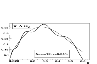
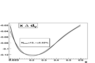
Figure 1: Results of $\Delta u_{V}(x)$ ($\alpha_{opt}=8.189221$, $\beta_{opt}=-0.99000$) and $\Delta d_{V}(x)$ ($\alpha_{opt}=-0.99000$, $\beta_{opt}=-0.387196$) reconstruction with the usual JEM. Solid line corresponds to the input (reference) parametrization GRSV2000NLO (symmetric sea). Dotted line corresponds to the distribution reconstructed with JEM for $N_{max}=12$.

where we put $F(x)=\Delta u_{V}(x)$ or $F(x)=\Delta d_{V}(x)$ and choose $a=0.023,b=0.6$ . Substituting these moments in the expansion Eq. (2) with $N_{max}=12$, we look for optimal values of parameters $\alpha$ and $\beta$ corresponding to the minimal deviation of reconstructed curves for $\Delta u_{V}(x)$ and $\Delta d_{V}(x)$ from the input (reference) curves corresponding to input parametrization. To find these optimal values $\alpha_{opt}$ and $\beta_{opt}$ we use the program MINUIT [15]. The results are presented in Fig. 1. Looking at Fig. 1, one can see that the curves strongly differ from each other even for the high number of used moments $N_{max}=12$.

Thus, the substitution of truncated moments instead of exact ones in the expansion (2) is a rather crude approximation at least for HERMES $x_{B}$ region. Fortunately it is possible to modify the standard JEM in a such way that new series contains the truncated moments instead of the full ones. The new expansion looks as (see the Appendix)

$$F(x)\simeq F_{N_{max}}(x)=\left(\frac{x-a}{b-a}\right)^{\beta}\left(1-\frac{x-a}{b-a}\right)^{\alpha}$$

$$\times\sum_{n=0}^{N_{max}}\Theta_{n}^{(\alpha,\beta)}\left(\frac{x-a}{b-a}\right)\sum_{k=0}^{n}c_{nk}^{(\alpha,\beta)}\frac{1}{(b-a)^{k+1}}\sum_{l=0}^{k}\frac{k!}{l!(k-l)!}M^{\prime}[l+1](-a)^{k-l},$$ (4)

where we use the notation Eq. (3) for the moments truncated to accessible for measurement $x_{B}$ region. It is of great importance that now in the expansion enter not the full (unavailable) but the truncated (accessible) moments. Thus, having at our disposal few first truncated moments extracted in NLO QCD (Eqs. (9) below), and applying MJEM, Eq. (2), one can reconstruct the local distributions in the accessible for measurement $x_{B}$ region.

To proceed let us clarify the important question about the boundary distortions. The deviations of reconstructed with MJEM, Eq. (2), $F_{N_{max}}$ from F near the boundary points are unavoidable since MJEM is correctly defined in the entire region $(a,b)$ except for the small vicinities of boundary points (see the Appendix). Fortunately, $F_{N_{max}}$ and F are in very good agreement in the practically entire accessible $x_{B}$ region, while the boundary distortions are easily identified and controlled since they are very sharp and hold in very small vicinities of the boundary points (see Figs. 2-4 below). In this section we, for clarity, explicitly show these distortions in all figures. In the next sections the all such distortions will be just cutted off.

Let us check how well MJEM works. To this end let us repeat the simple exercises with reconstruction of the known GRSV2000NLO (symmetric sea) parametrization and compare the results of $\Delta u_{V}(x)$ and $\Delta d_{V}(x)$ reconstruction with the usual JEM and with the proposed MJEM. To control the quality of reconstruction we introduce the parameter

$$\nu=\frac{\int_{a}^{b}dx|F_{reconstructed}(x)-F_{reference}(x)|}{\int_{a}^{b}dx|F_{reference}|}\cdot 100\%,$$ (5)

where $F_{reference}(x)$ corresponds to the input parametrization and $F_{reconstructed}(x)\equiv F_{N_{max}}(x)$ in Eq. (2). We first perform the reconstruction with very high number of moments $N_{max}=12$ and then with the small number $N_{max}=4$. Notice that the last choice $N_{max}=4$ is especially important because of peculiarities of the data on asymmetries provided by the SIDIS experiments. Indeed, the number of used moments should be as small as possible because first, the relative error $|\delta(M^{\prime}[j])/M^{\prime}[j]|$ on $M^{\prime}[j]$ becomes higher with increase of $j$ and second, the high moments become very sensitive to the replacement of integration by the sum over the bins. The results of $\Delta u_{V}(x)$ and $\Delta d_{V}(x)$ reconstruction with MJEM at $N_{max}=12$ and with application of both JEM and MJEM (in comparison) at $N_{max}=4$, are presented in Figs. 2 and 3. It is seen (see Fig. 2) that for $N_{max}=12$ MJEM, on the contrary to the usual JEM (see Fig. 1), gives the excellent agreement between the reference and reconstructed curves. In the case $N_{max}=4$ the difference in quality of reconstruction between JEM and MJEM (see Fig. 3) becomes especially impressive. While for standard JEM the reconstructed and reference curves strongly differ from each other, the respective curves for MJEM are in a good agreement. Thus, one can conclude that dealing with the truncated, available to measurement, $x_{B}$ region one should apply the proposed modified JEM to obtain the reliable results on the local distributions.

Until now we looked for the optimal values of parameters $\alpha$ and $\beta$ entering MJEM using explicit form of the reference curve (input parametrization). Certainly, in reality we have no any reference curve to be used for optimization. However, one can extract from the data in NLO QCD the first few moments (Eqs. (9) below). Thus, we need some criterion of MJEM optimization which would use for optimization of $\alpha$ and $\beta$ only the known (extracted) moments entering MJEM.

On the first sight it seems to be natural to find the optimal values of $\alpha$ and $\beta$ minimizing the difference of reconstructed with MJEM and input (entering MJEM (2)) moments. However, it is easy to prove (see the Appendix) that this difference is equal to zero:

$$M^{\prime}_{[a,b]}[n]{\Biggl{|}}_{\rm reconstructed}=M^{\prime}_{[a,b]}[n]{\Biggl{|}}_{input},\quad n\leq N_{max},$$ (6)

i.e. all reconstructed moments with $n\leq N_{max}$ are identically equal to the respective input moments for any $\alpha$ and $\beta$. Fortunately, we can use for comparison the reference “twice-truncated” moments

$$M^{\prime\prime}[n]\equiv M^{\prime\prime}_{[a+a^{\prime},b-b^{\prime}]}[n]\equiv\int_{a+a^{\prime}}^{b-b^{\prime}}dx\,x^{n-1}F(x)\quad(a<a+a^{\prime}<b-b^{\prime}<b),$$ (7)

i.e. the integrals over the region less than the integration region $(a,b)$ for the “once-truncated” moments $M^{\prime}_{[a,b]}$ entering MJEM (2). The respective optimization criterion can be written in the form

$$\sum_{j=0}^{N_{max}}{\Bigl{|}}M^{\prime\prime}_{\rm(reconstructed)}[j]-M^{\prime\prime}_{\rm(reference)}[j]{\Bigl{|}}=min.$$ (8)

The “twice truncated” reference moments should be extracted in NLO QCD from the data in the same way as the input (entering MJEM (2)) “once truncated” moments. In reality one can obtain “twice-truncated” moments using Eqs. (9) (below) and removing, for example, first and/or last bin from the sum in Eq. (14) (below).

Let us now check how well the optimization criterion (8) works. To this end we again perform the simple numerical test. We choose GRSV2000NLO parametrization at $Q^{2}=2.5\,GeV^{2}$ with both broken and symmetric sea scenarios. We then calculate four first “once-truncated” and four first “twice-truncated” moments defined by Eqs. (3) and (7), and then substitute them in Eq. (2) and the optimization criterion (8), respectively. To find the optimal values of $\alpha$ and $\beta$ we use the MINUIT [15] program. The results are presented in Fig. 4. It is seen that the optimization criterion works well for both symmetric and broken sea scenarios.

Thus, the performed numerical tests show that the proposed modification of the Jacobi polynomial expansion method allows to reconstruct with a high precision the quark helicity distributions in the accessible for measurement $x_{B}$ region.

3 Reconstruction of the valence quark helicity distributions from the simulated data.

In this section the proposed NLO QCD method will be applied to the simulated data. The simulations give us a good tool for testing of the method since here one knows in advance the answer to be found – the reference parametrization entering the generator as an input. At the same time the properly performed simulations (i.e., corresponding to the experimental statistics, binning and kinematical cuts) allow us finally adapt the method for application to the real experimental data.

Let us first investigate the peculiarities of the nth moments extraction in the conditions of the real experimental binning (rather small number of bins covering the accessible for measurement $x_{B}$ region).

The simple extension of the procedure proposed in Ref. [5] gives for the n-th moments $\Delta_{n}q\equiv\int_{0}^{1}dx\,x^{n-1}q(x)$ of the valence distributions the equations

$$\Delta_{n}u_{V}=\frac{1}{5}\frac{{\cal A}_{p}^{(n)}+{\cal A}_{d}^{(n)}}{L_{(n)1}-L_{(n)2}};\quad\Delta_{n}d_{V}=\frac{1}{5}\frac{4{\cal A}_{d}^{(n)}-{\cal A}_{p}^{(n)}}{L_{(n)1}-L_{(n)2}}.$$ (9)

Here the notation is absolutely analogous to one used in Ref. [5]:

$${\cal A}_{p}^{(n)}\equiv\int_{0}^{1}dx\ x^{n-1}A_{p}^{\pi^{+}-\pi^{-}}{\Biggl{|}}_{Z}(4u_{V}-d_{V})$$

$$\times\int_{Z}^{1}dz_{h}[1+\otimes\frac{\alpha_{s}}{2\pi}{C}_{qq}\otimes](D_{1}-D_{2}),$$ (10)

$${\cal A}_{d}^{(n)}\equiv\int_{0}^{1}dx\ x^{n-1}A_{d}^{\pi^{+}-\pi^{-}}{\Biggl{|}}_{Z}(u_{V}+d_{V})$$

$$\times\int_{Z}^{1}dz_{h}[1+\otimes\frac{\alpha_{s}}{2\pi}{C}_{qq}\otimes](D_{1}-D_{2}),$$ (11)

where $D_{1}$ ($D_{2}$) is favored (unfavored) pion fragmentation function, the quantities $L_{(n)1}$, $L_{(n)2}$ are defined as

$$L_{(n)1}\equiv L_{(n)u}^{\pi^{+}}=L_{(n)\bar{u}}^{\pi^{-}}=L_{(n)\bar{d}}^{\pi^{+}}=L_{(n)d}^{\pi^{-}},$$

$$L_{(n)2}\equiv L_{(n)d}^{\pi^{+}}=L_{{(n)}\bar{d}}^{\pi^{-}}=L_{(n)u}^{\pi^{-}}=L_{(n)\bar{u}}^{\pi^{+}},$$ (12)

$$L_{(n)q}^{h}\equiv\int_{Z}^{1}dz_{h}\left[D_{q}^{h}(z_{h})+\frac{\alpha_{s}}{2\pi}\int_{z_{h}}^{1}\frac{dz^{\prime}}{z^{\prime}}\ \Delta_{n}C_{qq}(z^{\prime})D_{q}^{h}(\frac{z_{h}}{z^{\prime}})\right],$$

where

$$\Delta_{n}C_{qq}(z)\equiv\int_{0}^{1}dx\ x^{n-1}\Delta C_{qq}(x,z)$$

are the nth moments of the polarized Wilson coefficients $\Delta C_{qq}(x,z)$ entering the NLO expressions for the difference asymmetries $A_{p,d}^{\pi^{+}-\pi^{-}}$ (the respective experimental expressions via counting rates are given by Eq. (19) – see below):

$$A_{p}^{\pi^{+}-\pi^{-}}(x,Q^{2}){\Bigl{|}}_{Z}=\frac{(4\Delta u_{V}-\Delta d_{V})\int_{Z}^{1}dz_{h}[1+\otimes\frac{\alpha_{s}}{2\pi}\Delta C_{qq}\otimes](D_{1}-D_{2})}{(4u_{V}-d_{V})\int_{Z}^{1}dz_{h}[1+\otimes\frac{\alpha_{s}}{2\pi}{C}_{qq}\otimes](D_{1}-D_{2})},$$

$$A_{d}^{\pi^{+}-\pi^{-}}(x,Q^{2}){\Bigl{|}}_{Z}=\frac{(\Delta u_{V}+\Delta d_{V})\int_{Z}^{1}dz_{h}[1+\otimes\frac{\alpha_{s}}{2\pi}\Delta C_{qq}\otimes](D_{1}-D_{2})}{(u_{V}+d_{V})\int_{Z}^{1}dz_{h}[1+\otimes\frac{\alpha_{s}}{2\pi}{C}_{qq}\otimes](D_{1}-D_{2})}.$$

It should be noticed that in reality one can measure the asymmetries only in the restricted Bjorken $x$ region $a<x<b$, so that the approximate equations for the truncated moments (c.f. Eq. (3))

$$\Delta^{\prime}_{n}q\equiv M^{\prime}[n]\equiv\int_{a}^{b}dx\,x^{n-1}\Delta q(x)$$ (13)

of the valence distributions have the form Eq. (9) with the replacement of the full integrals in Eq. (3) by the sums over bins covering the accessible region $a<x<b$:

$${\cal A}_{p}^{(n)}\simeq\sum_{i=1}^{N_{bins}}x^{n-1}\Delta x_{i}\,A_{p}^{\pi^{+}-\pi^{-}}(x_{i}){\Bigl{|}}_{Z}(4u_{V}-d_{V})(x_{i})\int_{Z}^{1}dz_{h}[1+\otimes\frac{\alpha_{s}}{2\pi}{C}_{qq}\otimes](D_{1}-D_{2}),$$ (14)

and analogously for ${\cal A}_{d}^{(n)}$.

The approximation to Eq. (3) given by Eq. (14) is based on the assumption that all integrated quantities are the constants within each bin. This is well-known “middle point” numerical integration method.

However, it seems that there is a way to improve this approximation having in mind the real experimental situation. The point is that the reality of an experiment compel us to approximate by the constant within the bin only the measured quantity (difference asymmetry here), that can be written as

$$A_{p}^{\pi^{+}-\pi^{-}}(x){\Bigl{|}}_{Z}=\sum_{i=1}^{N_{bins}}A_{p}^{\pi^{+}-\pi^{-}}(\langle x_{i}\rangle){\Bigl{|}}_{Z}\theta(x-x_{i-1})\theta(x_{i}-x),$$ (15)

where $A_{p}^{\pi^{+}-\pi^{-}}(\langle x_{i}\rangle){\Bigl{|}}_{Z}$ is the mean value of asymmetry in ith bin, $x_{0}=a$, $x_{N_{bins}}=b$ and $\theta(x)$ is the usual step function. At the same time, there is no any need to approximate by the constant another $x$-dependent quantities (unpolarized valence PDFs and Wilson coefficients here) entering the integrals over $x_{B}$ as the known input. Thus, substituting Eq. (15) in the initial integral equation Eq. (3) we get (c.f. Eq. (14))

$${\cal A}_{p}^{(n)}=\sum_{i=1}^{N_{bins}}A_{p}^{\pi^{+}-\pi^{-}}(\langle x_{i}\rangle){\Bigl{|}}_{Z}\int_{x_{i-1}}^{x_{i}}dxx^{n-1}(4u_{V}-d_{V})(x)\int_{Z}^{1}dz_{h}[1+\otimes\frac{\alpha_{s}}{2\pi}{C}_{qq}\otimes](D_{1}-D_{2}).$$ (16)

Notice that the analogous way of the integral approximation was applied by the HERMES collaboration in Ref. [2], where the moments $\Delta^{\prime}_{n}q$ were reconstructed substituting extracted from the data (“measured”) quantities $(\Delta q/q)(x_{i})$ in the equation (see Eq. (46) in Ref. [2])

$$\Delta^{\prime}_{n}q=\int_{0.023}^{0,6}dx\sum_{i=1}^{N_{bins}}\left[\frac{\Delta q}{q}(\langle x_{i}\rangle)\theta(x-x_{i-1})\theta(x_{i}-x)\right]x^{n-1}q(x).$$ (17)

To see the advantage of Eq. (16) application, let us compare it with the application of the integration procedure given by Eq. (14). To this end we perform absolutely idealized LO test, where in each bin (we choose the HERMES binning) the value of asymmetry is directly calculated from the given parametrization on $\Delta u_{V}$ and $\Delta d_{V}$ using the theoretical LO expressions [8] for the difference asymmetries

$$A_{p}^{\pi^{+}-\pi^{-}}=\frac{4\Delta u_{V}-\Delta d_{V}}{4u_{V}-d_{V}};\quad A_{d}^{\pi^{+}-\pi^{-}}=\frac{\Delta u_{V}+\Delta d_{V}}{u_{V}+d_{V}}.$$ (18)

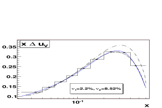
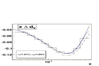
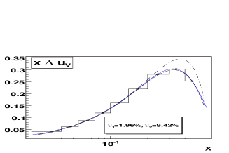
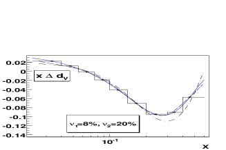
Figure 5: (color online) Idealized LO testing of the integration procedures given by Eq. (14) and Eq. (16). The input parametrizations GRSV2000LO with symmetric sea scenario (top) and broken sea scenario (bottom) are used for direct calculation of asymmetries with Eq. (18). Solid line corresponds to the input parametrization. Closed circles correspond to the values of input parametrization in the middle of each bin. Broken line shows the way of integral approximation corresponding to application of Eq. (14). Dashed line is obtained with MJEM and application of Eq. (16) for the moment calculation. Dot-dashed line is obtained with MJEM and application of Eq. (14) for the moment calculation. Parameters $\nu_{1}$ and $\nu_{2}$ are given by Eq. (5) and show the quality of reconstruction for the dashed and dot-dashed lines, respectively.

For simplicity, within this test we put $\langle x_{i}\rangle=(x_{i}-x_{i-1})/2$ ($i=1,\ldots,9;x_{0}=0.023,x_{9}=0.6$), so that reconstructed with Eq. (18) values of $\Delta u_{V}(\langle x_{i}\rangle)$ and $\Delta d_{V}(\langle x_{i}\rangle)$ exactly coincide with the respective input parametrization values in the points $\langle x_{i}\rangle$ – see Fig 5. Now we calculate four first moments using reduced to LO Eqs. (9) and the integration procedures given by Eqs. (14) and (16) and then we apply MJEM to both sets of the obtained moments. Looking at Fig. 5 one can see that reconstructed in this way curves strongly differ from each other, and the curve obtained with application of the integration procedure given by Eq. (16) is in much better agreement with the input (reference) parametrization.

Thus, following the results of just performed test, from now on we will use namely Eq. (16) performing the moments calculations.

Let us now perform LO and NLO analysis of the simulated SIDIS data on $\pi^{+}$ and $\pi^{-}$ production with both proton and deutron targets. To this end we use the PEPSI generator of polarized events [16]. The conditions of simulations are presented in Table 1 and correspond to the HERMES kinematics. Let us stress that all the cuts on $Q^{2}$, $x_{F}$, $W^{2}$ and $z_{h}$ in Table 1 are the standard physical cuts applied by SMC, HERMES and COMPASS. The statistics $3\cdot 10^{6}$ in Table 1 is the total number of DIS events for both proton and deutron targets and for both longitudinal polarizations.

Table 1: Simulation conditions. Here $x_{B}$ and $x_{F}$ are the Bjorken and Feynman variables, respectively, $z_{h}$ is the standard hadronic variable and $W$ is the invariant mass of the final hadronic state.

$E_{lepton}$	$x_{B}$	$x_{F}$	$z_{h}$
27.5 $GeV$	$0.023<x_{B}<0.6$	$x_{F}>0.1$	$z_{h}>Z=0.2$
$W^{2}$	$Q^{2}$	$Q^{2}_{mean}$	Events
$W^{2}>10\,GeV^{2}$	$Q^{2}>1\,GeV^{2}$	2.4 $GeV^{2}$	$3\cdot 10^{6}$

Using the simulated data we construct the difference asymmetries (see Ref. [5] for details)

$$A^{\pi^{+}-\pi^{-}}_{p(d)}{\Bigl{|}}_{Z}=\frac{1}{P_{B}P_{T}fD}\frac{(N^{\pi^{+}}_{\uparrow\downarrow}-N^{\pi^{-}}_{\uparrow\downarrow})L_{\uparrow\uparrow}-(N^{\pi^{+}}_{\uparrow\uparrow}-N^{\pi^{-}}_{\uparrow\uparrow})L_{\uparrow\downarrow}}{(N^{\pi^{+}}_{\uparrow\downarrow}-N^{\pi^{-}}_{\uparrow\downarrow})L_{\uparrow\uparrow}+(N^{\pi^{+}}_{\uparrow\uparrow}-N^{\pi^{-}}_{\uparrow\uparrow})L_{\uparrow\downarrow}},$$ (19)

where $N^{\pi^{\pm}}_{\uparrow\downarrow(\uparrow\uparrow)}$ are the counting rates integrated over $z_{h}$ in the region $Z=0.2<z_{h}<1$, $L_{\uparrow\downarrow(\uparrow\uparrow)}=N_{\uparrow\downarrow(\uparrow\uparrow)}/\sigma_{\uparrow\downarrow(\uparrow\uparrow)}$ are the luminosities, and the quantities $p_{B}$, $p_{T}$, $f$ are equal to unity in the conditions of simulations with PEPSI.

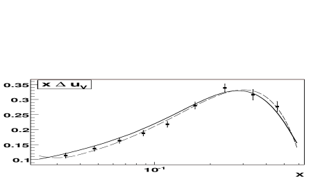
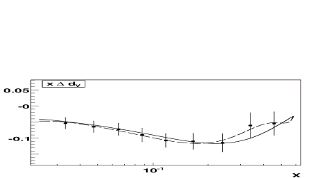
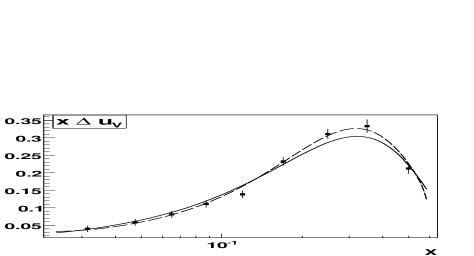
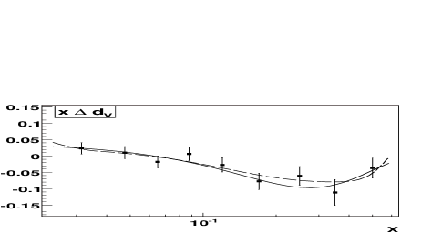
Figure 6: Results of the simulated difference asymmetry analysis in LO. GRSV2000LO parametrizations for symmetric sea (top) and broken sea (bottom) scenarios are used for simulations. Solid line corresponds to the input parametrization. Dashed line corresponds to the reconstructed with MJEM curve. Points with error bars correspond to direct extraction of the valence distributions with Eq. (18).

We first perform the LO analysis of the simulated difference asymmetries. The important peculiarity of LO analysis is that in this case one can perform the extraction of $\Delta u_{V}$ and $\Delta d_{V}$ in two ways. First is the direct extraction where one applies Eqs. (18) in each bin – points with error bars in Fig. 6. The second method is the proposed one, where MJEM is applied to the LO extracted moments – dashed line in Fig. 6. The moments used in MJEM are extracted from the simulated difference asymmetries with application of reduced to LO Eqs. (9-3), (16) and are presented in Table 2.

Table 2: Results for LO extracted truncated moments for the simulations with the entering PEPSI two different parametrizations: GRSV2000LO (symmetric sea) parametrization (top) and GRSV2000LO (broken sea) parametrization (bottom). For comparison the respective reference (obtained by direct integration of entering PEPSI input parametrizations) moments are also presented.

	$\Delta^{\prime}_{n}u_{V}$		$\Delta^{\prime}_{n}d_{V}$
n	Extracted	Reference	Extracted	Reference
1	0.7042 $\pm$ 0.0124	0.7176	-0.2568 $\pm$ 0.0271	-0.2618
2	0.1489 $\pm$ 0.0037	0.1477	-0.0439 $\pm$ 0.0079	-0.0482
3	0.0467 $\pm$ 0.0016	0.0457	-0.0118 $\pm$ 0.0033	-0.0135
4	0.0179 $\pm$ 0.0007	0.0173	-0.0041 $\pm$ 0.0015	-0.0048
	$\Delta^{\prime}_{n}u_{V}$		$\Delta^{\prime}_{n}d_{V}$
n	Extracted	Reference	Extracted	Reference
1	0.5346 $\pm$ 0.0123	0.5255	-0.0952 $\pm$ 0.0274	-0.1103
2	0.1318 $\pm$ 0.0036	0.1282	-0.0297 $\pm$ 0.0081	-0.0331
3	0.0434 $\pm$ 0.0015	0.0425	-0.0098 $\pm$ 0.0034	-0.0107
4	0.0167 $\pm$ 0.0007	0.0166	-0.0037 $\pm$ 0.0015	-0.0039

Looking at Fig. 6, one can see that the input (reference) parametrization slightly deviates from both the directly extracted values of $\Delta u_{V}$ and $\Delta d_{V}$ and the reconstructed with MJEM curve. These deviations are unavoidable and are caused by the specific character of the events generation with PEPSI. Our experience shows that the asymmetries reconstructed from the generated events always slightly differ from the respective asymmetries calculated from the input parametrizations (with application of Eq. (18) in LO). One the other hand, comparing the directly extracted and the reconstructed with MJEM $\Delta u_{V}$ and $\Delta d_{V}$, one can see that they are in a good agreement with each other. Thus, the performed LO testing encourage us that the proposed method of PDFs extraction could be successfully applied.

Let us now clarify the important point concerning application of the optimization criterion Eq. (8) which we use to find the optimal values $\alpha_{opt}$ and $\beta_{opt}$ of the entering MJEM parameters $\alpha$ and $\beta$ (see Section 2 for details). All over the paper, applying the optimization criterion, we simultaneously use for each $j$ ($j=1,\ldots 4$) in the sum two extracted twice-truncated moments. These moments correspond to two (sufficiently large and overlapping) integration regions, covering respectively the bins from first to seven and from third to last ninth. We make such choice because on the one hand, one should take into account in the criterion the whole accessible integration region, and, on the other hand, the “twice-truncated” moments should essentially differ from the “once truncated” moments for the well-working of the minimization procedure (see the respective discussion just after Eq. (6)).

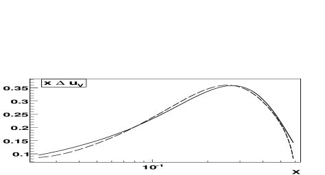
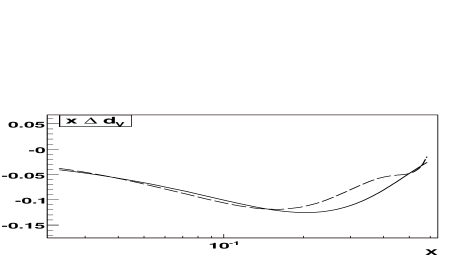
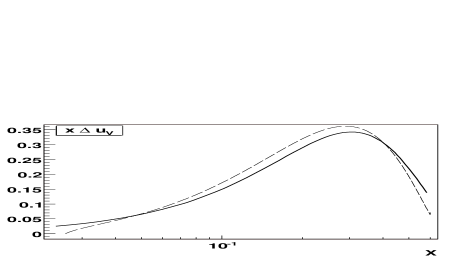
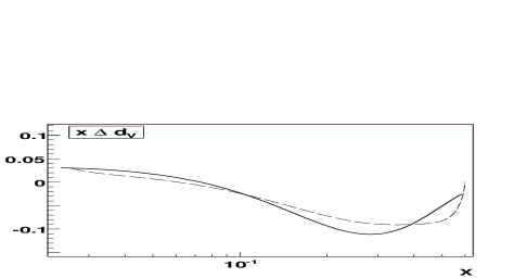
Figure 7: Results of the simulated difference asymmetry analysis in NLO. GRSV2000NLO parametrizations for symmetric sea (top) and broken sea (bottom) scenarios are used for simulations. Solid line corresponds to the input parametrization. Dashed line corresponds to the reconstructed with MJEM curve.

Let us now perform the NLO analysis of the simulated data. We again use as an input two different parametrizations GRSV2000NLO (symmetric sea) and GRSV2000NLO (broken sea). The conditions of simulation are presented in Table 1. We first extract the truncated moments using Eqs. (9)-(3) and (16). The results are presented in Table 3. Using these moments and applying MJEM, we reconstruct in NLO $\Delta u_{V}(x)$ and $\Delta d_{V}(x)$ with the results presented in Fig. 7. Comparing Fig. 7 with Fig. 6, one can see that quality of reconstruction in NLO is not worse than the quality of LO reconstruction. The slight deviations of reconstructed and input curves as before (c.f. Fig. 6) are explained by the unavoidable deviations of the simulated with PEPSI asymmetries from their reference (corresponding to the input parametrization) values.

Table 3: Results for NLO extracted truncated moments for the simulations with the entering PEPSI two different parametrizations: GRSV2000NLO (symmetric sea) parametrization (top) and GRSV2000NLO (broken sea) parametrization (bottom). For comparison the respective reference (obtained by direct integration of entering PEPSI input parametrizations) moments are also presented.

	$\Delta^{\prime}_{n}u_{V}$		$\Delta^{\prime}_{n}d_{V}$
n	Extracted	Reference	Extracted	Reference
1	0.7369 $\pm$ 0.0133	0.7507	-0.2577 $\pm$ 0.0293	-0.2760
2	0.1507 $\pm$ 0.0039	0.1545	-0.0423 $\pm$ 0.0085	-0.0490
3	0.0449 $\pm$ 0.0016	0.0471	-0.0109 $\pm$ 0.0033	-0.0133
4	0.0163 $\pm$ 0.0007	0.0176	-0.0037 $\pm$ 0.0015	-0.0045
	$\Delta^{\prime}_{n}u_{V}$		$\Delta^{\prime}_{n}d_{V}$
n	Extracted	Reference	Extracted	Reference
1	0.5860 $\pm$0.0134	0.5701	-0.1045 $\pm$0.0300	-0.1137
2	0.1392 $\pm$0.0039	0.1381	-0.0314 $\pm$0.0088	-0.0367
3	0.0433 $\pm$0.0015	0.0448	-0.0101 $\pm$0.0034	-0.0121
4	0.0159 $\pm$0.0007	0.0172	-0.0037 $\pm$0.0016	-0.0045

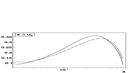
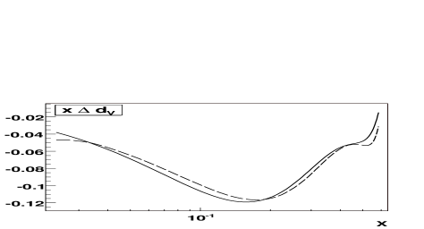
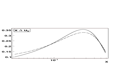
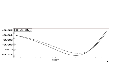
Figure 8: Combined results of LO and NLO analysis (top) of the simulated difference asymmetries in comparison with the respective LO and NLO versions of GRSV2000 (symmetric sea) parametrization (bottom). Dashed and solid lines correspond to LO and NLO curves, respectively.

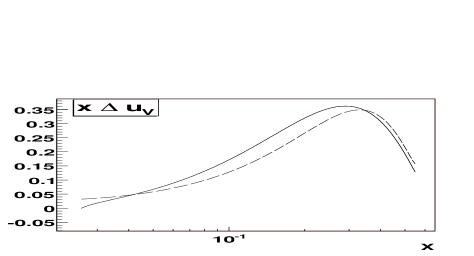
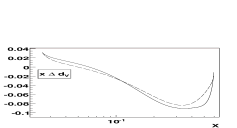
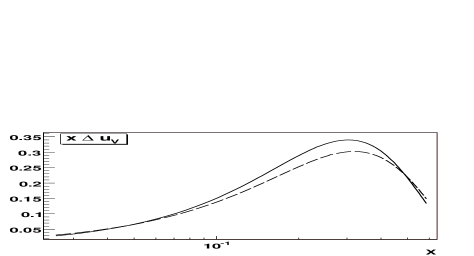
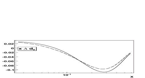
Figure 9: Combined results of LO and NLO analysis (top) of the simulated difference asymmetries in comparison with the respective LO and NLO versions of GRSV2000 (broken sea) parametrization (bottom). Dashed and solid lines correspond to LO and NLO curves, respectively.

The remark concerning very important peculiarity of application in NLO of the optimization criterion Eq. (8) should be made here. The crucial point for the optimization criterion is the proper choice of the initial values of $\alpha$ and $\beta$. Indeed, the experience shows that if these initial values are too far away from the real $\alpha_{opt}$ and $\beta_{opt}$ to be found, then the MINUIT program can “fall” into some wrong local minimum and produce the false values of $\alpha_{opt}$ and $\beta_{opt}$. Fortunately in LO we can compare the reconstructed with MJEM curve with the reference (directly extracted) values of PDFs and unambiguously find the optimal values of $\alpha_{opt}$ and $\beta_{opt}$. On the other hand, it is natural to use $\alpha_{opt}$ and $\beta_{opt}$ obtained within LO analysis as the initial (starting) values for the application of optimization criterion Eq. (8) in NLO. The simulations demonstrate (see Fig. 7) that with the such choice of initial $\alpha$ and $\beta$ the minimization procedure performed in NLO analysis unambiguously finds the proper values of $\alpha_{opt}$ and $\beta_{opt}$. As a result the obtained with MJEM curves are in a good agreement with the input (reference) parametrizations. At the same time, looking at Figs. 8 and 9, one can see that the behavior of both LO and NLO extracted curves is in a good agreement with the respective behavior of the input (reference) parametrizations.

Thus, all performed in this section studies show that the proposed method can be successfully applied to the polarized PDFs extraction in NLO QCD.

4 NLO QCD analysis of the HERMES data on pion production.

4.1 Construction of the difference asymmetries from the HERMES data on pion production

Let us now apply the proposed method to the HERMES SIDIS data on the pion production. Within this paper we would like first of all to test the applicability of the method to the experimental data analysis. That is why, for a moment, we do not like to deal with the such poorly known objects as $D_{q}^{K^{\pm}}$ and $D_{g}^{h}$ fragmentation functions. As it was discussed before (see the Introduction), from this point of view the most attractive objects are the difference asymmetries. At the same time the difference asymmetries are still not constructed. So, let us apply a trick and express the difference asymmetry given by Eq. (19) via the standard virtual photon SIDIS asymmetries

$$A_{p(d)}^{\pi^{\pm}}{\Bigl{|}}_{Z}=\frac{1}{P_{B}P_{T}fD}\frac{N^{\pi^{\pm}}_{\uparrow\downarrow}L_{\uparrow\uparrow}-N^{\pi^{\pm}}_{\uparrow\uparrow}L_{\uparrow\downarrow}}{N^{\pi^{\pm}}_{\uparrow\downarrow}L_{\uparrow\uparrow}+N^{\pi^{\pm}}_{\uparrow\uparrow}L_{\uparrow\downarrow}},$$

which were measured by HERMES [2]. Namely, in each ith bin the difference asymmetries given by Eq. (19) can be rewritten as

$$A^{\pi^{+}-\pi^{-}}(x_{i})=\frac{R_{i}^{+/-}}{R_{i}^{+/-}-1}A^{\pi^{+}}(x_{i})-\frac{1}{R_{i}^{+/-}-1}A^{\pi^{-}}(x_{i}),$$ (20)

where the quantity $R^{+/-}_{i}$ is defined as

$$R^{+/-}_{i}\equiv\frac{N^{\pi^{+}}_{i\uparrow\downarrow}L_{\uparrow\uparrow}+N^{\pi^{+}}_{i\uparrow\uparrow}L_{\uparrow\downarrow}}{N^{\pi^{-}}_{i\uparrow\downarrow}L_{\uparrow\uparrow}+N^{\pi^{-}}_{i\uparrow\uparrow}L_{\uparrow\downarrow}}.$$

It is easy to see that the ratio $R^{+/-}_{i}$ can be rewritten as

$$R^{+/-}_{i}=\frac{\sigma^{\pi^{+}}_{\uparrow\downarrow}(x_{i})+\sigma^{\pi^{+}}_{\uparrow\uparrow}(x_{i})}{\sigma^{\pi^{-}}_{\uparrow\downarrow}(x_{i})+\sigma^{\pi^{-}}_{\uparrow\uparrow}(x_{i})}=\frac{\sigma^{\pi^{+}}_{unpol}(x_{i})}{\sigma^{\pi^{-}}_{unpol}(x_{i})}=\frac{N^{\pi^{+}}_{i}}{N^{\pi^{-}}_{i}},$$ (21)

and, thus, can be taken from the unpolarized SIDIS data. This relative quantity is well defined and extracted with the high precision object. We take its value from the LEPTO generator of unpolarized events [17], which gives a good description of the fragmentation processes. The calculations show that the relative quantities $R_{i}^{+/-}$ remarkably weakly depend on statistics of simulated events. Indeed, if one changes $N_{total}^{\pi^{+}}{\Bigl{|}}_{LEPTO}$ from $10^{5}$ to $10^{6}$ then only 1-3% deviation of $R^{+/-}_{i}$ (in dependence of bin number) occurs. Nevertheless, to be more precise, extracting the quantities $R_{i}^{+/-}$ for the HERMES statistics ($N^{\pi^{+}}_{total}=117.000$, $N^{\pi^{-}}_{total}=82.000$ for proton and $N^{\pi^{+}}_{total}=491.000$, $N^{\pi^{-}}_{total}=385.000$ for deutron targets, respectively [2]) we preserve the condition

$$N^{\pi^{\pm}}_{total}{\Bigl{|}}_{LEPTO}\simeq N^{\pi^{\pm}}_{total}{\Bigl{|}}_{HERMES},\quad N_{total}^{\pi^{\pm}}\equiv\sum\nolimits_{i}N_{i}^{\pi^{\pm}},$$ (22)

performing the simulations with LEPTO. The results for $R_{i}^{+/-}$ are presented in Table 4.

Table 4: The obtained from the LEPTO generator results for the relative unpolarized quantity $R_{i}^{+/-}$ given by Eq. (21).

	proton target	deutron target
$i$	$R^{+/-}_{i}$	$R^{+/-}_{i}$
1	1.220	1.150
2	1.270	1.201
3	1.346	1.229
4	1.436	1.274
5	1.494	1.315
6	1.569	1.350
7	1.629	1.407
8	1.669	1.444
9	1.803	1.556

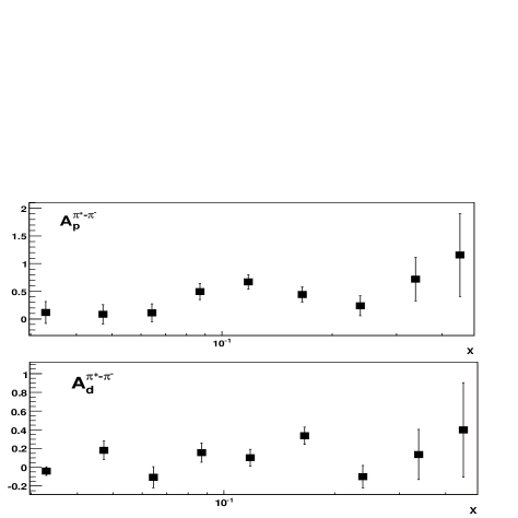
Figure 10: Difference asymmetries constructed with application of Eq. (20).

Thus, using in Eq. (20) the results from Table 4 and HERMES results [2] on $A_{p,d}^{\pi^{\pm}}$ (see Tables XII and XIII in Ref. [2]), one easily constructs the difference asymmetries $A_{p,d}^{\pi^{+}-\pi^{-}}$. The results are presented in Fig. 10.

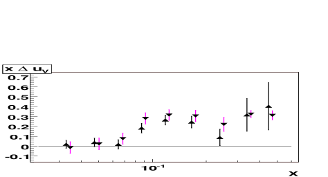
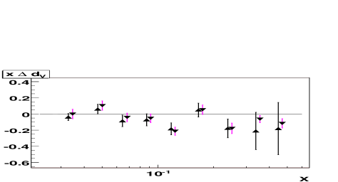
Figure 11: (color online) LO extraction of the valence PDFs from the difference asymmetries constructed with Eq. (20) (up-oriented triangles) in comparison with the respective published HERMES results (down-oriented triangles). The HERMES results are shifted to the right for better visibility.

First, for the sake of testing (to check how well Eq. (20) works), we reconstruct the valence PDFs in the leading order. In LO the equations for the difference asymmetries take the simple form given by Eq. (18). With these equations we reconstruct $\Delta u_{V}$ and $\Delta d_{V}$ using the results on difference asymmetries presented in Fig. 10. The results are shown in Fig. 11 , where we also plotted the respective results from Ref. [2] (obtained with the purity method). One can see that the results obtained with both procedures are in a good agreement.

Let us now compare the LO extracted moments (truncated to the HERMES $x_{B}$ region) obtained with application of Eq. (20) (first line in the Table 5 ) with the existing LO results of SMC and HERMES taken from the Table XI in Ref. [2]. One can see that the results obtained with application of Eq. (20) (i.e., from the difference asymmetries plotted in Fig. 10 ) are in a good accordance with both HERMES and SMC results.

Table 5: LO extracted truncated moments obtained from the difference asymmetries constructed with application of Eq. (20) in comparison with the existing LO results of SMC and HERMES collaborations.The SMC moments are truncated to the HERMES $x_{B}$ region and are evolved to the HERMES $Q^{2}_{mean}=2.5\,GeV^{2}$ – see Table XI in Ref. [2].

$\Delta^{\prime}_{n}u_{V}$
n	1	2	3	4
This paper	0.510 $\pm$ 0.110	0.134$\pm$0.043	0.048 $\pm$ 0.020	0.020 $\pm$ 0.010
HERMES	0.603 $\pm$ 0.071	0.144$\pm$0.014	-/-	-/-
SMC	0.614 $\pm$ 0.082	0.152$\pm$0.016	-/-	-/-
$\Delta^{\prime}_{n}d_{V}$
n	1	2	3	4
This paper	-0.280$\pm$0.146	-0.074$\pm$ 0.058	-0.026 $\pm$ 0.026	-0.011 $\pm$ 0.013
HERMES	-0.172$\pm$0.068	-0.047$\pm$ 0.012	-/-	-/-
SMC	-0.334$\pm$0.112	-0.056$\pm$ 0.026	-/-	-/-

Thus, the performed LO tests show that representation Eq. (20) for the difference asymmetry can be successfully applied.

Notice also that even the LO extraction of $\Delta u_{V}$ and $\Delta d_{V}$ from the difference asymmetries is interesting in itself as an alternative (complementary) possibility. Indeed, Eqs. (18) are free from the rather badly known fragmentation functions and purities.

4.2 Reconstruction of the valence PDFs in NLO QCD

Here, using the constructed difference asymmetries as a starting point and operating just as in Section 3, we will reconstruct in NLO QCD both the truncated Mellin moments of the valence PDFs and the local PDFs themselves.

Let us first extract four first moments truncated to the HERMES $x_{B}$ region. The results are presented in Table 6. It is of importance that the proposed procedure allows us to extract the moments in NLO directly, without the commonly used assumptions like $\Delta\bar{u}=\Delta\bar{d}=\Delta s=\Delta\bar{s}$ (see, for example, Refs. [14, 18]). Notice that the first moments $\Delta_{1}u_{V}$ and $\Delta_{1}d_{V}$ are very important in themselves because namely the first moments compose the nucleon spin. At the same time all four moments presented in Table 6 are necessary for the reconstruction of the local PDFs with MJEM application.

Table 6: NLO extracted truncated moments obtained from the difference asymmetries constructed with application of Eq. (20).

n	1	2	3	4
$\Delta^{\prime}_{n}u_{V}$	0.555 $\pm$ 0.126	0.134 $\pm$ 0.047	0.047 $\pm$ 0.020	0.019 $\pm$ 0.10
$\Delta^{\prime}_{n}d_{V}$	-0.302 $\pm$ 0.173	-0.076 $\pm$ 0.064	-0.025 $\pm$ 0.027	-0.010 $\pm$ 0.012

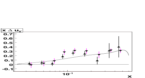
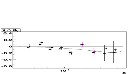
Figure 12: (color online) Different LO procedures of the valence PDFs extraction in comparison. Solid line and up-oriented triangles correspond to LO extraction with the proposed method and direct extraction with Eq. (18), respectively. The difference asymmetries constructed with application of Eq. (20) are used. Down-oriented triangles correspond to LO results of HERMES obtained with application of the purity method to the measured by HERMES usual virtual photon spin asymmetries.

Before application of MJEM in NLO, let us, for the sake of testing, reconstruct the local valence distributions in the leading order using LO moments from Table 5. The results are presented in Fig. 12. One can see that reconstructed with MJEM Eq. (2) and optimization criterion Eq. (8) curve is in a good agreement with both HERMES results and with the results of direct LO extraction from the difference asymmetries constructed with application of Eq. (20).

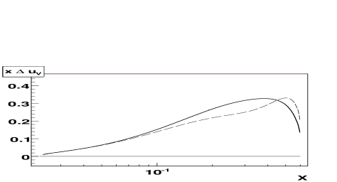
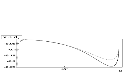
Figure 13: Results of both LO and NLO analysis of the difference asymmetries constructed with Eq. (20). Solid and dashed lines correspond to NLO and LO results, respectively.

After the successful LO testing we apply MJEM in NLO QCD using the results for $\Delta^{\prime}_{n}u_{V}$ and $\Delta^{\prime}_{n}d_{V}$ from Table 6. The results are presented in Fig. 13, where also, for comparison, the respective LO results are plotted. It is seen that the behavior of NLO and LO curves with respect to each other is in agreement with the predictions of existing parametrizations (see, for example, [14]).

4.3 Corrections caused by $Q^{2}$ dependence of asymmetries

Until now we applied the approximation

$$A(x_{i},Q_{i}^{2})\simeq A(x_{i},Q_{\rm mean}^{2})$$

commonly used (see Refs. [1, 2]) for analysis of the DIS and SIDIS asymmetries. This approximation is in a good agreement even with the COMPASS data (see Fig. 5 in Ref. [19]) and is especially suitable for the HERMES kinematics, where the “shoulder” in $Q^{2}$ is rather small ($1\,GeV^{2}\;\raisebox{-1.72218pt}{\tiny$\stackrel{{\scriptstyle{\textstyle<}}}{{\sim}}$}\;Q^{2}\;\raisebox{-1.72218pt}{\tiny$\stackrel{{\scriptstyle{\textstyle<}}}{{\sim}}$}\;10\,GeV^{2}$; $Q^{2}_{mean}=2.5\,GeV^{2}$ – see Tables XII and XIII in Ref. [2]) in comparison with the SMC and COMPASS kinematics. Nevertheless, even for the HERMES kinematics we deal with, for more comprehensive analysis, it is useful to estimate the corrections caused by the weak $Q^{2}$ dependence of the difference asymmetries. So, let us estimate the shifts in all four NLO moments caused by the respective shifts

$$\delta_{i}A_{p,d}^{\pi^{+}-\pi^{-}}=A_{p,d}^{\pi^{+}-\pi^{-}}(x_{i},Q^{2}_{mean})-A_{p,d}^{\pi^{+}-\pi^{-}}(x_{i},Q_{i}^{2})$$ (23)

in the difference asymmetries. The most simple way to estimate $\delta_{i}A_{p,d}^{\pi^{+}-\pi^{-}}$ is to use the maximal number of the latest available NLO parametrizations. Namely, we approximate r.h.s of Eq. (23) by the respective difference of “theoretical” asymmetries calculated with substitution of the different parametrizations to NLO equations for the difference asymmetries – Eqs. (14), (15) in Ref. [5].

Adding the calculated in this way $\delta_{i}A_{p,d}^{\pi^{+}-\pi^{-}}$ to the initial experimental asymmetries $A_{p,d}^{\pi^{+}-\pi^{-}}(x_{i},Q_{i}^{2})$, one estimates the evolved from $Q_{i}^{2}$ to $Q^{2}_{mean}$ asymmetries $A_{p,d}^{\pi^{+}-\pi^{-}}(x_{i},Q_{mean}^{2})|_{Evolved}$. Using the obtained in such a way evolved asymmetries we extract the respective corrected moments of the valence PDFs $\Delta^{\prime}_{n}q_{V}|_{Corrected}$ repeating the procedure from Section 3. Then we compare the corrected moments $\Delta^{\prime}_{n}q_{V}|_{Corrected}$ with the respective moments $\Delta^{\prime}_{n}q_{V}$ from the previous section (obtained without corrections due to evolution) and calculate the respective shifts $\delta(\Delta^{\prime}_{n}q_{V})=\Delta^{\prime}_{n}q_{V}|_{Corrected}-\Delta^{\prime}_{n}q_{V}$. The results are presented in the Tables 7 and 8, where also the relative quantities $\delta(\Delta^{\prime}_{n}q_{V})/\Delta^{\prime}_{n}q_{V}$ are presented.

Table 7: NLO results for $\Delta^{\prime}_{n}u_{V}$ corrected due to evolution (top) together with the respective absolute and relative deviations from the uncorrected moments (bottom). The corrections are estimated using seven different NLO parametrizations. The roman numbers I and II correspond to GRSV2000NLO parametrization for broken and symmetric sea scenarios, respectively. The roman numbers III and IV correspond to Ref. [21] for sets ii+ and ii- (symmetric and weakly broken sea scenarios). The rest of numbers V-VII corresponds to the NLO parametrizations from Ref. [18] (in the order of citation).

$\Delta^{\prime}_{n}u_{V}|_{Corrected}$
n	I	II	III	IV	V	VI	VII
1	0.5495	0.5464	0.5555	0.5551	0.5473	0.5588	0.5457
2	0.1364	0.1367	0.1378	0.1377	0.1368	0.1387	0.1363
3	0.0459	0.0460	0.0463	0.0463	0.0460	0.0467	0.0459
4	0.0182	0.0182	0.0183	0.0183	0.0182	0.0185	0.0182
Average $\Delta^{\prime}_{n}u_{V}|_{Corrected}$
n
1	0.5437 $\pm$ 0.1266
2	0.1348 $\pm$ 0.0475
3	0.0453 $\pm$ 0.0199
4	0.0179 $\pm$ 0.0089
$\delta(\Delta^{\prime}_{n}u_{V})$
n	I	II	III	IV	V	VI	VII
1	-0.0054	-0.0085	0.0006	0.0002	-0.0077	0.0039	-0.0092
2	-0.0034	-0.0031	-0.0019	-0.0021	-0.0030	-0.0010	-0.0035
3	-0.0013	-0.0012	-0.0009	-0.0009	-0.0012	-0.0005	-0.0013
4	-0.0005	-0.0005	-0.0004	-0.0004	-0.0005	-0.0002	-0.0006
$\delta(\Delta^{\prime}_{n}u_{V})/\Delta^{\prime}_{n}u_{V}$ (%)
n	I	II	III	IV	V	VI	VII
1	-0.97	-1.53	0.11	0.04	-1.38	0.71	-1.65
2	-2.42	-2.21	-1.37	-1.47	-2.12	-0.73	-2.47
3	-2.67	-2.54	-1.86	-1.95	-2.56	-1.14	-2.84
4	-2.62	-2.62	-2.08	-2.14	-2.72	-1.28	-2.94
Average $\delta(\Delta^{\prime}_{n}u_{V})$
n
1	-0.0037
2	-0.0026
3	-0.0011
4	-0.0004

Notice that the considered procedure of the asymmetry evolution is quite similar to the procedure used by SMC for the $\Gamma_{1p(d)}$ reconstruction (see Section V in Ref. [20]).

Table 8: NLO results for $\Delta^{\prime}_{n}d_{V}$ corrected due to evolution (top) together with the respective absolute and relative deviations from the uncorrected moments (bottom). The corrections are estimated using seven different NLO parametrizations. The roman numbers I and II correspond to GRSV2000NLO parametrization for broken and symmetric sea scenarios, respectively. The roman numbers III and IV correspond to Ref. [21] for sets ii+ and ii- (symmetric and weakly broken sea scenarios). The rest of numbers V-VII corresponds to the NLO parametrizations from Ref. [18] (in the order of citation).

$\Delta^{\prime}_{n}d_{V}|_{Corrected}$
n	I	II	III	IV	V	VI	VII
1	-0.3130	-0.3091	-0.3197	-0.3251	-0.3062	-0.3096	-0.3064
2	-0.0778	-0.0779	-0.0811	-0.0822	-0.0771	-0.0780	-0.0774
3	-0.0256	-0.0256	-0.0267	-0.0269	-0.0254	-0.0256	-0.0255
4	-0.0096	-0.0098	-0.0102	-0.0102	-0.0097	-0.0097	-0.0097
Average $\Delta^{\prime}_{n}d_{V}|_{Corrected}$
n
1	-0.3127 $\pm$0.1731
2	-0.0788 $\pm$0.0643
3	-0.0259 $\pm$0.0269
4	-0.0099 $\pm$0.0119
$\delta(\Delta^{\prime}_{n}d_{V})$
n	I	II	III	IV	V	VI	VII
1	-0.0114	-0.0075	-0.0181	-0.0235	-0.0046	-0.0080	-0.0048
2	-0.0015	-0.0017	-0.0048	-0.0059	-0.0008	-0.0018	-0.0012
3	-0.0003	-0.0004	-0.0014	-0.0017	-0.0001	-0.0003	-0.0002
4	-0.0001	-0.0001	-0.0005	-0.0006	-0.0000	-0.0000	-0.0000
$\delta(\Delta^{\prime}_{n}d_{V})/\Delta^{\prime}_{n}d_{V}$ (%)
n	I	II	III	IV	V	VI	VII
1	3.77	2.48	5.99	7.78	1.53	2.65	1.58
2	1.97	2.20	6.33	7.72	1.10	2.33	1.53
3	1.31	1.47	5.71	6.74	0.52	1.35	0.95
4	0.83	0.83	5.07	5.89	0.10	0.52	0.52
Average $\delta(\Delta^{\prime}_{n}d_{V})$
n
1	-0.0111
2	-0.0025
3	-0.0007
4	-0.0002

It is of importance that we use for estimations the set of essentially different NLO parametrizations and some of them, for example GRSV2000 (broken sea) and GRSV2000 (symmetric sea), differ from each other very strongly. However, one can see from the Tables 7, 8 that independently of the chosen parametrization the corrections for moments caused by evolution are very small (negligible in comparison with the statistical errors). To be precise, one can just include $\delta(\Delta^{\prime}_{n}q_{V})|_{Average}$ (see Tables 7 and 8) in the systematical error.

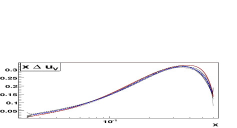
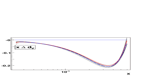
Figure 14: (color online) NLO results obtained with application of MJEM to the moments extracted from the difference asymmetries corrected due to evolution. Dotted lines correspond to corrections estimated with the different parametrizations. Dashed line corresponds to the curve averaged over corrections. Solid line corresponds to reconstruction without corrections.

Let us now reconstruct the local valence PDFs applying MJEM to the corrected moments $\Delta^{\prime}_{n}q_{V}|_{Corrected}$ from the Tables 7 and 8. The results are presented in Fig. 14. One can see that the curves corresponding to the different ways of correction (different used parametrizations) are very close to each other. The averaged over the different corrections curve (dashed line) also very insignificantly differs from the initial (obtained without corrections) curve (solid line).

Thus, the performed in this Section analysis demonstrates that at least for the HERMES kinematics we deal with here, the results are very insensitive to the corrections on the difference asymmetries caused by evolution.

5 Conclusions and prospects

Thus, in this paper the method of polarized SIDIS data analysis in NLO QCD is developed. The main peculiarity of the method is that its application is based on two subsequently applied procedures. First one directly extracts in NLO few first truncated (available to measurement) Mellin moments of the quark helicity distributions. The obtained at this stage results are very important and interesting in themselves. Indeed, the first moments are the main objects for understanding of the nucleon spin structure since they compose the nucleon spin. Second, using the obtained at first stage truncated moments as an input to the modification of the Jacobi polynomial expansion method, one eventually reconstructs the local quark helicity distributions in the accessible for measurement $x_{B}$ region.

After successful testing we apply the proposed NLO method to the HERMES data on the pion production. To this end the pion difference asymmetries are constructed for both proton and deutron targets. To construct the difference asymmetries we use the HERMES data on the usual virtual photon SIDIS asymmetries, and, also, the well known quantity – ratio of unpolarized cross-sections for $\pi^{+}$ and $\pi^{-}$ production which we take from the LEPTO generator of unpolarized events. With the constructed in such a way difference asymmetries the LO results of the valence distribution reconstruction are in a good accordance with the respective leading order HERMES and SMC results, while the NLO results are in agreement with the existing NLO parametrizations on these quantities. Nevertheless, the obtained results should be considered as the rather preliminary since we construct the difference asymmetries in indirect way. At present the difference asymmetries are constructed by HERMES and are expected to be available in the nearest future. Certainly, it is very desirable to perform the NLO analysis of these directly constructed asymmetries and compare the results with the respective results presented in this paper.

In this paper we apply the proposed method to the difference asymmetries only. Let us recall once again that essential advantage of these asymmetries in comparison with any other ones is the absence of fragmentation functions in LO and the weak dependence of well known difference of favored and unfavored pion fragmentation functions in NLO. So, since within this paper we mainly would like to investigate how well the method itself works, we, for a moment, prefer to deal namely with these very clean (from theoretical point of view) objects. In this connection it is of importance that the measurement of the difference asymmetries is one of the main topics of the physical program of E04-113 experiment planned at Jefferson Lab [22]. It is of importance that in this experiment the expected average $Q^{2}$ is also rather small (about $2\,GeV^{2}$). So, the NLO analysis in this experiment is also strongly required.

Certainly, in the nearest future we will apply the method to NLO analysis of all measured in the SIDIS experiments asymmetries. In particular, it can allow us to extract in NLO so important quantity as the polarized strangeness in nucleon. Regretfully, the only existing today data on kaon production (HERMES experiment) suffers of large statistical errors and, besides, the accessible for measurement HERMES $x_{B}$ region is rather narrow. So, to obtain the reliable results on the such tiny quantity as $\Delta_{1}s$ (as well as on $\Delta_{1}\bar{u}$ and $\Delta_{1}\bar{d}$) it is necessary to perform the combined analysis, i.e., to analyze in NLO the combined data of SMC, HERMES, COMPASS and the planned E04-113 (Jefferson Lab) experiments. This is one of the main subjects of our future investigations.

6 Acknowledgments

The authors are grateful to N. Akopov, E.C. Aschenauer, R. Bertini, M.P. Bussa, O. Denisov, D. Hasch, H.E. Jackson, A. Korzenev, V. Krivokhizhin, E. Kuraev, A. Maggiora, C.A. Miller, A. Nagaytsev, A. Olshevsky, G. Piragino, G. Pontecorvo, I. Savin, A. Sidorov, O. Teryaev and R. Windmolders, for fruitful discussions. The work of O.S and O.I. was supported by the Russian Foundation for Basic Research (project no. 05-02-17748).

Appendix

JEM is the expansion of $x$-dependent function (structure function or quark density) in the series over Jacobi polynomials $\Theta^{(\alpha,\beta)}_{n}(x)$ orthogonal with weight $\omega^{(\alpha,\beta)}(x)=x^{\beta}(1-x)^{\alpha}$ (see [11] -[10] for details):

$$F(x)\simeq F_{N_{max}}(x)=\omega^{(\alpha,\beta)}\sum\nolimits_{k=0}^{N_{max}}\Theta_{k}^{(\alpha,\beta)}(x)$$

$$\times\sum\nolimits_{j=0}^{k}c_{kj}^{{(\alpha,\beta)}}M(j+1),$$ (A.1)

where

$$M[j]=\int_{0}^{1}dx\,x^{j-1}F(x)$$ (A.2)

and

$$\int_{0}^{1}dx\omega^{(\alpha,\beta)}(x)\Theta^{(\alpha,\beta)}_{n}(x)\Theta^{(\alpha,\beta)}_{m}(x)=\delta_{nm}.$$ (A.3)

The details on the Jacobi polynomials

$$\Theta_{k}^{(\alpha,\beta)}(x)=\sum_{j=0}^{k}c_{kj}^{(\alpha,\beta)}x^{j}$$ (A.4)

can be found in Refs. [11] and [12]. In practice one truncates the series (6) living in the expansion only finite number of moments $N_{max}$ – see Eq. (2). The experience shows [10] that even small $N_{max}$ gives good results.

The idea of modified expansion is to reexpand $F(x)$ in the series over the truncated moments $M^{\prime}_{[ab]}[j]$ given by Eq. (3), performing the rescaling $x\rightarrow a+(b-a)x$ which compress the entire region $[0,1]$ to the truncated region $[a,b]$. To this end let us apply the following ansatz

$$F(x)=\left(\frac{x-a}{b-a}\right)^{\beta}\left(1-\frac{x-a}{b-a}\right)^{\alpha}\sum_{n=0}^{\infty}\tilde{f}_{n}\Theta_{n}^{(\alpha,\beta)}\left(\frac{x-a}{b-a}\right)$$ (A.5)

and try to find the coefficients $\tilde{f}_{n}$. Multiplying both parts of Eq. (A.5) by $\Theta_{k}^{(\alpha,\beta)}((x-a)/(b-a))$, integrating over x in the limits $[a,b]$ and performing the replacement $t=(x-a)/(b-a)$, one gets

$$\int_{a}^{b}dx\,F(x)\Theta_{k}^{(\alpha,\beta)}\left(\frac{x-a}{b-a}\right)=(b-a)\sum_{n=0}^{\infty}{\tilde{f}_{n}}\int_{0}^{1}dt\,t^{\beta}(1-t)^{\alpha}\Theta_{n}^{(\alpha,\beta)}(t)\Theta_{k}^{(\alpha,\beta)}(t),$$ (A.6)

so that with the orthogonality condition Eq. (A.3) one obtains

$$\tilde{f}_{n}=(b-a)^{-1}\int_{a}^{b}dx\,F(x)\Theta_{n}^{(\alpha,\beta)}\left(\frac{x-a}{b-a}\right).$$ (A.7)

Substituting Eq. (A.7) in the expansion (A.5), and using Eq. (A.4) one eventually gets

$$F(x)=\left(\frac{x-a}{b-a}\right)^{\beta}\left(1-\frac{x-a}{b-a}\right)^{\alpha}$$

$$\times\sum_{n=0}^{\infty}\Theta_{n}^{(\alpha,\beta)}\left(\frac{x-a}{b-a}\right)\sum_{k=0}^{n}c_{nk}^{(\alpha,\beta)}\frac{1}{(b-a)^{k+1}}\sum_{l=0}^{k}\frac{k!}{l!(k-l)!}M^{\prime}_{[a,b]}[l+1](-a)^{k-l},$$ (A.8)

where $M^{\prime}_{[a,b]}[j]$ is given by Eq. (3). Truncating in the exact Eq. (6) the infinite sum over $n$ to the sum $\sum_{n=0}^{N_{max}}$ one gets the approximate equation (2).

Let us prove the important property of the truncated moments reconstructed with MJEM.

For any $n\leq N_{max}$

$$M^{\prime}_{[a,b]}[n+1]{\Biggl{|}}_{reconstructed}=M^{\prime}_{[a,b]}[n+1]{\Biggl{|}}_{input},$$ (A.9)

where

$$M^{\prime}_{[a,b]}[n]{\Biggl{|}}_{input}=\int_{a}^{b}dxx^{n-1}F(x),\quad M^{\prime}_{[a,b]}[n]{\Biggl{|}}_{reconstructed}=\int_{a}^{b}dxx^{n-1}F_{N_{max}}(x),$$ (A.10)

$F_{N_{max}}(x)$ is the function reconstructed with application of MJEM (2), and $N_{max}+1$ is the number of the highest of moments used in Eq. (2).

To prove this statement we will need the inverse to (A.4) expansion

$$x^{n}=\sum_{k=0}^{n}d_{nk}^{(\alpha,\beta)}\Theta_{k}^{(\alpha,\beta)}(x),$$ (A.11)

with the obvious property of $d_{nk}^{(\alpha,\beta)}$ coefficients

$$\sum_{k=j}^{n}d_{nk}^{(\alpha,\beta)}c_{kj}^{(\alpha,\beta)}=\delta_{nj}.$$ (A.12)

Let us integrate Eq. (2) over $x$ in the limits $[a,b]$ with weight $((x-a)/(b-a))^{n}$.

$$\int_{a}^{b}dx\left(\frac{x-a}{b-a}\right)^{n}F_{N_{max}}(x)=$$

$$\int_{a}^{b}dx\left(\frac{x-a}{b-a}\right)^{n}\left\{\omega^{(\alpha,\beta)}\left(\frac{x-a}{b-a}\right)\sum_{m=0}^{N_{max}}\Theta_{m}^{(\alpha,\beta)}\left(\frac{x-a}{b-a}\right)\right.$$

$$\left.\times(b-a)^{-1}\sum_{j=0}^{m}c_{mj}^{(\alpha,\beta)}\int_{a}^{b}dz\,F(z)\left(\frac{z-a}{b-a}\right)^{j}\right\}.$$ (A.13)

Using expansion (A.11) and orthogonality condition (A.3), one easily gets

$$\int_{a}^{b}dx\left(\frac{x-a}{b-a}\right)^{n}F_{N_{max}}(x)=$$

$$\sum_{m=0}^{N_{max}}\sum_{k=0}^{n}\delta_{km}\left[d_{nk}^{(\alpha,\beta)}\sum_{j=0}^{m}c_{mj}^{(\alpha,\beta)}\int_{a}^{b}dx\,F(x)\left(\frac{x-a}{b-a}\right)^{j}\right].$$ (A.14)

It is obvious that at $n\leq N_{max}$ the Kronecker symbol $\delta_{km}$ reduces the sum $\sum_{m=0}^{N_{max}}$ to the sum $\sum_{m=0}^{n}$. Thus, summing over $m$ with $\delta_{km}$, using the identity

$$\sum_{k=0}^{n}\sum_{j=0}^{k}f_{jk}\equiv\sum_{j=0}^{n}\sum_{k=j}^{n}f_{jk}$$ (A.15)

and applying Eq. (A.12), one get eventually:

$$\int_{a}^{b}dx\left(\frac{x-a}{b-a}\right)^{n}F_{N_{max}}(x)=\int_{a}^{b}dx\left(\frac{x-a}{b-a}\right)^{n}F(x),\quad{n\leq N_{max}}$$ (A.16)

Setting $n=0$ in Eq. (A.16) one obtains

$$M^{\prime}_{[a,b]}[1]{\Biggl{|}}_{reconstructed}\equiv\int_{a}^{b}dx\,F_{N_{max}}(x)=\int_{a}^{b}dx\,F(x)\equiv M^{\prime}_{[a,b]}[1]{\Biggl{|}}_{input}.$$ (A.17)

Putting then $n=1$ in (A.16) and using (A.17) one gets

$$M^{\prime}_{[a,b]}[2]{\Biggl{|}}_{reconstructed}=M^{\prime}_{[a,b]}[2]{\Biggl{|}}_{input}.$$ (A.18)

Operating in this way for all $n\leq N_{max}$, one arrives at the equality (A.9) to be proved.

In conclusion, very important remark should be made here. Notice that ansatz (A.5) (as well as the expansion Eq. (2) itself) is correctly defined inside the entire region $(a,b)$ except for the small vicinities of boundary points (absolutely the same situation holds for the usual JEM, Eq. (6), applied to the quark distributions in the region $(0,1)$). Thus, near the boundary points the deviations of reconstructed with MJEM function from its true values are unavoidable. Fortunately, all numerical examples (see section 2) show that input and reconstructed with MJEM functions are in very good agreement in the practically entire considered $x_{B}$ region, while the boundary distortions are easily identified and controlled since they are very sharp and hold in very small vicinities of the boundary points (see Figs. 2-4). Thus, to reconstruct the curve near the boundary points one should just cut off these distortions and then extrapolate the rest to the boundaries of the considered $x_{B}$ region.

To be precise, it should be also noticed that the all proofs given in the Appendix are rather formal because of the boundary distortions problem. All equations in the Appendix (like, for example, Eq. (A.9)) become exact only when the distortions are cutted off and extrapolation to the boundaries is made. Fortunately, the practice show that the distortion regions are so small that the numerical results on the integrals over the entire region $[a,b]$ are practically insensitive to the way of extrapolation, so that all equations in the Appendix are valid with a high numerical precision.

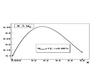
Figure 2: Results of $\Delta u_{V}(x)$ ($\alpha_{opt}=-0.827885$, $\beta_{opt}=-0.011505$) and $\Delta d_{V}(x)$ ($\alpha_{opt}=-0.989752$, $\beta_{opt}=-0.012393$) reconstruction with MJEM. Solid line corresponds to the input (reference) parametrization GRSV2000NLO (symmetric sea). Dotted line corresponds to the distribution reconstructed with MJEM for $N_{max}=12$.

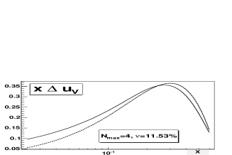
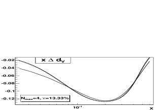
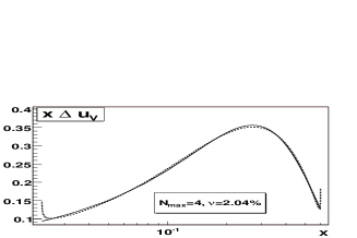
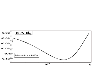
Figure 3: Results of the valence PDFs reconstruction with JEM and MJEM in comparison. Top part corresponds to $\Delta u_{V}(x)$ ($\alpha_{opt}=-0.99$, $\beta_{opt}=0.054010$) and $\Delta d_{V}(x)$ ($\alpha_{opt}=0.174096$, $\beta_{opt}=0.162567$) reconstructed with the usual JEM. Bottom part corresponds to $\Delta u_{V}(x)$ ($\alpha_{opt}=-0.0025869$, $\beta_{opt}=-0.071591$) and $\Delta d_{V}(x)$ ($\alpha_{opt}=0.110331$, $\beta_{opt}=-0.049255$) reconstructed with MJEM. Solid lines correspond to input (reference) parametrization GRSV2000NLO (symmetric sea). Dotted lines correspond to the distributions reconstructed with JEM (top) and MJEM (bottom).

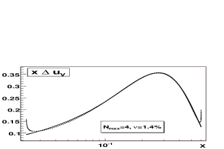
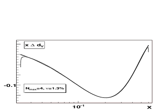
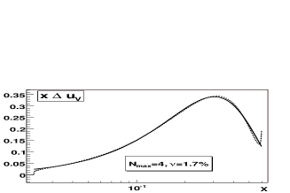
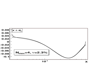
Figure 4: Results of $\Delta u_{V}$ and $\Delta d_{V}$ reconstruction for GRSV2000NLO parametrization for both symmetric (top) and broken sea (bottom) scenarios. Solid line corresponds to the reference curve (input parametrization). Dotted line is reconstructed with MJEM and criterion (8) inside the accessible for measurement region ([0.023,0.6] here). Optimal values of parameters for symmetric sea scenario for $\Delta u_{V}$ are $\alpha_{opt}=-0.15555$, $\beta_{opt}=-0.097951$ and for $\Delta d_{V}$ are $\alpha_{opt}=-0.002750$, $\beta_{opt}=-0.07190$. Optimal values of parameters for broken sea scenario for $\Delta u_{V}$ are $\alpha_{opt}=-0.209346$, $\beta_{opt}=0.153417$ and for $\Delta d_{V}$ are $\alpha_{opt}=0.702699$, $\beta_{opt}=-0.293231$.

References

- [1] SMC collaboration (B. Adeva et al.), Phys. Lett. B 369 (1996) 93
- [2] HERMES collaboration (A. Airapetyan et al.), Phys. Rev. D71 (2005) 012003
- [3] COMPASS collaboration (G. Baum et al.), ”COMPASS: A proposal for a common muon and proton apparatus for structure and spectroscopy”, CERN-SPSLC-96-14 (1996).
- [4] A.N. Sissakian, O.Yu. Shevchenko and O.N. Ivanov, Phys. Rev. D68 (2003) 031502
- [5] A.N. Sissakian, O.Yu. Shevchenko and O.N. Ivanov, Phys. Rev. D70 (2004) 074032
- [6] A.N. Sissakian, O.Yu. Shevchenko and O.N. Ivanov, JETP Lett. 82 (2005) 53
- [7] D. de Florian, G.A. Navarro, R. Sassot, Phys. Rev. D71 (2005) 094018
- [8] L. Frankfurt et al, Phys. Lett. B 230 (1989) 141
- [9] E. Christova and E. Leader, hep-ph/0007303.
- [10] V.G. Krivokhizhin et al, Z. Phys. C36 (1987) 51; JINR-E2-86-564
- [11] G. Parisi, N. Sourlas, Nucl. Phys. B151 (1979) 421
- [12] I.S. Barker, C.S. Langensiepen, G. Shaw, Nucl. Phys. B186 (1981) 61; CERN-TH-2988
- [13] E. Leader, A.V. Sidorov, D.B. Stamenov, Int. J. Mod. Phys. A13 (1998) 5573
- [14] M. Gluck, E. Reya, M. Stratmann, W. Vogelsang, Phys. Rev. D63 (2001) 094005; hep-ph/0011215
- [15] F. James, M. Roos, Comput. Phys. Commun. 10 (1975) 343
- [16] L. Mankiewicz, A. Schafer, M. Veltri, Comput. Phys. Commun. 71 (1992) 305
- [17] G. Ingelman, A. Edin, J. Rathsman, Comput. Phys. Commun. 101 (1997) 108.
-
[18]
Asymmetry Analysis collaboration (Y. Goto et al.), Phys. Rev. D 62 (2000) 034017;
E. Leader, A. Sidorov, D. Stamenov, Eur. Phys. J. C23 (2002) 479
Asymmetry Analysis Collaboration (M. Hirai et al.), Phys. Rev. D69 (2004) 054021 - [19] COMPASS Collaboration (E.S. Ageev et al.), Phys. Lett. B612 (2005) 154
- [20] SMC collaboration (B. Adeva et al), Phys. Rev. D58 (1998) 112002
- [21] D. de Florian, O.A. Sampayo, R. Sassot, Phys. Rev. D 57 (1998) 5803
- [22] X. Jiang et al., hep-ex/0412010