Improvement of the $\Theta^{+}$ width estimation method on the Light Cone

Recently, Diakonov and Petrov have suggested a formalism in the Chiral Quark Soliton Model allowing one to derive the 3-, 5-, 7-, …quark wavefunctions for the octet, decuplet and antidecuplet. They have used this formalism and many strong approximations in order to estimate the exotic $\Theta^{+}$ width. The latter has been estimated to $\sim$4 MeV. Besides they obtained that the 5-quark component of the nucleon is about 50% of its 3-quark component meaning that relativistic effects are not small. We have improved the technique by taking into account some relativistic corrections and considering the previously neglected 5-quark exchange diagrams. We also have computed all nucleon axial charges. It turns out that exchange diagrams affect very little Diakonov’s and Petrov’s results while relativistic corrections reduce the $\Theta^{+}$ width to $\sim$2 MeV and the 5- to 3-quark component of the nucleon ratio to 30%.

1 Introduction

Diakonov and Petrov have derived an effective low-energy Lagrangian within their instanton model of the QCD vacuum [1]. This Lagrangian is presented in Section 2. It enjoys all symmetries of chiral QCD, deals with appropriate degrees of freedom and is believed to reproduce fairly well low-energy QCD physics. Even though this Lagrangian is a strong simplification of the original QCD Lagrangian, it is still a considerable task to solve it. In order to have some insights, the authors have developed a mean field approach to the problem. A mean field approach is usually justified by the large number of participants. For example, the Thomas-Fermi model of atoms is justified at large $Z$ [2]. For baryons, the number of colors $N_{C}$ has been used as such parameter [3]. Since $N_{C}=3$ in the real world, one can wonder how accurate is the mean field approach. The chiral field experiences fluctuations about its mean-field value of the order of $1/N_{C}$. These are loop corrections which are further suppressed by factors of $1/2\pi$ yielding to corrections typically of the order of 10%. These are ignored. However, rotations of the baryon mean field in ordinary and flavor spaces are not small for $N_{C}=3$ and are taken into account exactly.

The view that there is a self-consistent mean chiral field in baryons which binds three constituent quarks [4] is adopted in this paper. The binding is rather strong: bound-state quarks are relativistic and their wavefunction has both the upper $s$-wave Dirac component and the lower $p$-wave Dirac component, see Section 3. At the same time, the Dirac sea is distorted by this mean chiral field leading to the presence of an indefinite number of additional $q\bar{q}$ pairs in baryons. Ordinary baryons are then superpositions of 3-, 5-, 7-, …quark Fock components. These additional non-perturbative quark-antiquark pairs are essential for the understanding of the spin crisis and the nucleon $\sigma$ term [5, 6]. The former experimental value is three times smaller and the latter one is four times larger than the 3-quark theoretical value [7]. This picture of baryons has been called the Chiral Quark Soliton Model ($\chi$QSM). It leads without any fitting parameters to a reasonable quantitative description of baryon properties [4, 8], including nucleon parton distributions at low normalization point [9] and other baryon characteristics [10]. The model supports full relativistic invariance and all symmetries following from QCD.

As mentioned above, the only 3-quark picture of baryons is too simplistic since it cannot explain some experimental values. It is then well accepted that one has to consider the effect of additive quark-antiquark pairs. The problem is now quantitative. A simple perturbative amount is not sufficient indicating that the non-perturbative amount is important. $\chi$QSM allows one to address those questions since it naturally incorporates all additive quark-antiquark pairs in its description of baryons. On the top of that, since those additive quark-antiquark pairs are collective excitations of the mean chiral field, an extra pair costs little energy. In a recent paper [11] Diakonov and Petrov have estimated the 5-quark component in the nucleon and found that it is roughly 50% of the 3-quark component, and thus not small. The 3-quark picture of the nucleon is then definitely too simplistic.

The quantization of the rotation of the mean chiral field in the ordinary and flavor spaces yields to correct quantum numbers for the lowest baryons [3]. The rotated mean chiral field can be represented by $U(\mathbf{x})=RV(\mathbf{x})R^{\dagger}$ where $R$ is a $SU(3)$ rotation matrix. For simplicity, we deal with $m_{s}=0$. In this limit any rotated field is classically as good as the unrotated one. At the quantum level, the mean chiral field experiences rotations which cannot be considered as small since there is no cost of energy (zero modes). These rotations should be quantized properly. As first pointed out by Witten [3] and then derived using different techniques by a number of authors [12], the quantization rule is such that the lowest baryon multiplets are the octet with spin 1/2 and the decuplet with spin 3/2 followed by the exotic antidecuplet with spin 1/2. All of those multiplets have same parity. The lowest baryons are just rotational excitations of the same mean chiral field (soliton). They are distinguished by their specific rotational wavefunctions given explicitly in Section 4.

In this approach, most of low-energy properties of the lowest baryons follow from the shape of the mean chiral field in the classical baryon. The difference and splitting between baryons are exclusively due to the difference in their rotational wavefunctions, difference that can be translated into the quark wavefunctions of the individual baryons, both in the infinite momentum [13, 14] and the rest [15] frames. In Section 3 we recall the compact general formalism how to find the 3-, 5-, 7-, …quark wavefunctions inside the octet, decuplet and antidecuplet baryons and give further details on the ingredients in Sections 4, 5 and 6. In Section 7 the 3-quark wavefunctions of the octet and decuplet are shown. In the non-relativistic limit they are similar to the old $SU(6)$ quark wavefunctions but with well-defined relativistic corrections. The 5-quark wavefunctions of ordinary and exotic baryons are presented in Section 8.

We consider baryons in the Infinite Momentum Frame (IMF) since this is the only frame in which one can distinguish genuine quark-antiquark pairs of the baryon wavefunctions from vacuum fluctuations. Therefore an accurate definition of what are the 3-, 5-,7-, …quark Fock components of baryons can be made only in the IMF. Another advantage of such a frame is that the vector and axial charges with a finite momentum transfer do not create or annihilate quarks with infinite momenta. The baryon matrix elements are thus diagonal in the Fock space.

QCD does not forbid states made of more than 3 quarks as long as they are colorless. It was first expected that pentaquarks, i.e. particles which minimal quark content is four quarks and one antiquark, have wide widths [16, 17] and then difficult to observe experimentally. Later, some theorists have suggested that particular quark structures might exist with a narrow width [18, 19]. The experimental status on the existence of the exotic $\Theta^{+}$ pentaquark is still unclear. There are many experiments in favor (mostly low energy and low statistics) and against (mostly high energy and high statistics). A review on the experimental status can be found in [20, 21, 22]. Concerning the experiments in favor, they all agree that the $\Theta^{+}$ width is small but give only upper values. It turns out that if it exists, the exotic $\Theta^{+}$ has a width of the order of a few MeV or maybe even less than 1 MeV, a really curious property since usual resonance widths are of the order of 100 MeV. In the paper [19] that actually motivated experimentalists to search a pentaquark, Diakonov, Petrov and Polyakov have estimated the $\Theta^{+}$ width to be less than 15 MeV. More recently, Diakonov and Petrov used the present technique based on light-cone baryon wavefunction to estimate more accurately the width and have found that it turns out to be $\sim 4$ MeV [11] and then the view of a narrow pentaquark resonance within the $\chi$QSM is safe and appears naturally without any parameter fixing. However, many approximations have been used such as non-relativistic limit and omission of some 5-quark contributions (exchange diagrams). The authors expected that these have high probability to reduce further the width. This is what has motivated our work. We have improved the technique in order to include previously neglected diagrams in the 5-quark sector and some relativistic corrections to the discrete-level wavefunction.

Since the exotic $\Theta^{+}$ has no 3-quark component and that axial transitions are diagonal in the Fock space, one has to compute the 5-quark component of the nucleon and the $\Theta^{+}$. We should add in principle the contribution coming from the 7-, 9-, …quark sectors. They are neglected in the present paper. One way to control the approximation is through the computation of the nucleon axial charges. The 3-quark values are too crude. The 5-quark contributions bring the values nearer to experimental ones.

This paper is supposed to be self-consistent. In Sections 9 and 10 we remind how to compute the 3- and 5-quark contributions. We then improve the technique by taking into account the exchange diagrams and some relativistic corrections to the discrete-level wavefunction. In section 11 we collect all old [11] and new formal results on the strange axial current between the $\Theta^{+}$ and the nucleon and complete the set of nucleon axial charges. In Section 12 we give the numerical evaluation of those observables along with an estimation of the $\Theta^{+}$ width. It appears that exchange diagrams, oppositely to what was expected in [11] have little effect. However relativistic corrections lead to a reduction of the $\Theta^{+}$ width to $\sim 2$ MeV and the 5- to 3-quark component of the nucleon ratio to 30%.

2 The effective action of the Chiral Quark Soliton Model

$\chi$QSM is assumed to mimic low-energy QCD thanks to an effective action describing constituent quarks with a momentum dependent dynamical mass $M(p)$ interacting with the scalar $\Sigma$ and pseudoscalar $\boldsymbol{\Pi}$ fields. The chiral circle condition $\Sigma^{2}+\boldsymbol{\Pi}^{2}=1$ is invoked. The momentum dependence of $M(p)$ serves as a formfactor of the constituent quarks and provides also the effective theory with the UV cutoff. At the same time, it makes the theory non-local as one can see in the action

$$S_{\textrm{eff}}=\int\frac{\mathrm{d}^{4}p\,\mathrm{d}^{4}p^{\prime}}{(2\pi)^{8}}\,\bar{\psi}(p)\left[p\!\!\!/\,(2\pi)^{4}\delta^{(4)}(p-p^{\prime})-\sqrt{M(p)}(\Sigma(p-p^{\prime})+i\Pi(p-p^{\prime})\gamma_{5})\sqrt{M(p^{\prime})}\right]\psi(p^{\prime})$$ (1)

where $\psi$ and $\bar{\psi}$ are quarks fields. This action has been originally derived in the instanton model of the QCD vacuum [1]. Note that oppositely to naive bag picture, this equation (1) is fully relativistic and supports all general principles and sum rules for conserved quantities.

The formfactors $\sqrt{M(p)}$ cut off momenta at some characteristic scale which corresponds in the instanton picture to the inverse average size of instantons $1/\bar{\rho}\approx 600$ MeV. This means that in the range of quark momenta $p\ll 1/\bar{\rho}$ one can neglect the non-locality. We use the standard approach: the constituent quark mass is replaced by a constant $M=M(0)$ and we mimic the decreasing function $M(p)$ by the UV Pauli-Villars cutoff [9]

$$S_{\textrm{eff}}=\int\frac{\mathrm{d}^{4}p}{(2\pi)^{4}}\,\bar{\psi}(p)(p\!\!\!/-MU^{\gamma_{5}})\psi(p)$$ (2)

with $U^{\gamma_{5}}$ a $SU(3)$ matrix

$$U^{\gamma_{5}}=\left(\begin{array}[]{cc}U_{0}&0\\ 0&1\end{array}\right),\qquad U_{0}=e^{i\pi^{a}\tau^{a}\gamma_{5}}$$ (3)

and $\tau^{a}$ being usual $SU(2)$ Pauli matrices.

We are now going to remind the general technique from [11] that allows one to derive the (ligth-cone) baryon wavefunctions.

3 Explicit baryon wavefunction

In $\chi$QSM it is easy to define the baryon wavefunction in the rest frame. Indeed, this model represents quarks in the Hartree approximation in the self-consistent pion field. The baryon is then described as $N_{C}$ valence quarks + Dirac sea in that self-consistent external field. It has been shown [13] that the wavefunction of the Dirac sea is the coherent exponential of the quark-antiquark pairs

$$|\Omega\rangle=\exp\left(\int(\mathrm{d}\mathbf{p})(\mathrm{d}\mathbf{p}^{\prime})\,a^{\dagger}(\mathbf{p})W(\mathbf{p},\mathbf{p}^{\prime})b^{\dagger}(\mathbf{p}^{\prime})\right)|\Omega_{0}\rangle$$ (4)

where $|\Omega_{0}\rangle$ is the vacuum of quarks and antiquarks $a,b\,|\Omega_{0}\rangle=0$, $\langle\Omega_{0}|\,a^{\dagger},b^{\dagger}=0$ defined for the quark mass $M\approx 345$ MeV (known to fit numerous observables within the instanton mechanism of spontaneous chiral symmetry breaking [1]), $(\mathrm{d}\mathbf{p})=\mathrm{d}^{3}\mathbf{p}/(2\pi)^{3}$ and $W(\mathbf{p},\mathbf{p}^{\prime})$ is the quark Green function at equal times in the background $\Sigma,\boldsymbol{\Pi}$ fields [13, 14] (its explicit expression is given in section 5). In the mean field approximation the chiral field is replaced by the following spherically-symmetric self-consistent field

$$\pi(\mathbf{x})=\mathbf{n}\cdot\tau\,P(r),\qquad\mathbf{n}=\mathbf{x}/r,\qquad\Sigma(\mathbf{x})=\Sigma(r).$$ (5)

We then have on the chiral circle $\Pi=\mathbf{n}\cdot\tau\sin P(r)$, $\Sigma(r)=\cos P(r)$ with $P(r)$ being the profile function of the self-consistent field. The latter is fairly approximated by [4, 5] (see Fig. 2)

$$P(r)=2\arctan\left(\frac{r_{0}^{2}}{r^{2}}\right),\qquad r_{0}\approx\frac{0.8}{M}.$$ (6)

Such a chiral field creates a bound-state level for quarks, whose wavefunction $\psi_{\textrm{lev}}$ satisfies the static Dirac equation with eigenenergy $E_{\textrm{lev}}$ in the $K^{p}=0^{+}$ sector with $K=T+J$ [4, 23, 24]

$$\psi_{\textrm{lev}}(\mathbf{x})=\left(\begin{array}[]{c}\epsilon^{ji}h(r)\\ -i\epsilon^{jk}(\mathbf{n}\cdot\sigma)^{i}_{k}\,j(r)\end{array}\right),\qquad\left\{\begin{array}[]{c}h^{\prime}+h\,M\sin P-j(M\cos P+E_{\textrm{lev}})=0\\ j^{\prime}+2j/r-j\,M\sin P-h(M\cos P-E_{\textrm{lev}})=0\end{array}\right.$$ (7)

where $i=1,2=\uparrow,\downarrow$ and $j=1,2=u,d$ are respectively spin and isospin indices. Solving those equations with the self-consistent field (5) one finds that “valence” quarks are tightly bound ($E_{\textrm{lev}}=200$ MeV) along with a lower component $j(r)$ smaller than the upper one $h(r)$ (see Fig. 2).

Figure 1: Profile of the self-consistent chiral field $P(r)$ in light baryons. The horizontal axis unit is $r_{0}=0.8/M=0.46$ fm.

Figure 2: Upper $s$-wave component $h(r)$ (solid) and lower $p$-wave component $j(r)$ (dashed) of the bound-state quark level in light baryons. Each of the three valence quarks has energy $E_{\textrm{lev}}=200$ MeV. Horizontal axis has units of $1/M=0.57$ fm.

For the valence quark part of the baryon wavefunction it suffices to write the product of $N_{C}$ quark creation operators that fill in the discrete level [13]

$$\prod_{\textrm{color}=1}^{N_{C}}\int(\mathrm{d}\mathbf{p})F(\mathbf{p})a^{\dagger}(\mathbf{p})$$ (8)

where $F(\mathbf{p})$ is obtained by expanding and commuting $\psi_{\textrm{lev}}(\mathbf{p})$ with the coherent exponential (4)

$$F(\mathbf{p})=\int(\mathrm{d}\mathbf{p}^{\prime})\sqrt{\frac{M}{\epsilon}}[\bar{u}(\mathbf{p})\gamma_{0}\psi_{\textrm{lev}}(\mathbf{p})(2\pi)^{3}\delta^{(3)}(\mathbf{p}-\mathbf{p}^{\prime})-W(\mathbf{p},\mathbf{p}^{\prime})\bar{v}(\mathbf{p}^{\prime})\gamma_{0}\psi_{\textrm{lev}}(-\mathbf{p}^{\prime})].$$ (9)

One can see from the second term that the distorted Dirac sea contributes to the one-quark wavefunction. For the plane-wave Dirac bispinor $u_{\sigma}(\mathbf{p})$ and $v_{\sigma}(\mathbf{p})$ we used the standard basis

$$u_{\sigma}(\mathbf{p})=\left(\begin{array}[]{c}\sqrt{\frac{\epsilon+M}{2M}}s_{\sigma}\\ \sqrt{\frac{\epsilon-M}{2M}}\frac{\mathbf{p}\cdot\sigma}{|\mathbf{p}|}s_{\sigma}\end{array}\right),\qquad v_{\sigma}(\mathbf{p})=\left(\begin{array}[]{c}\sqrt{\frac{\epsilon-M}{2M}}\frac{\mathbf{p}\cdot\sigma}{|\mathbf{p}|}s_{\sigma}\\ \sqrt{\frac{\epsilon+M}{2M}}s_{\sigma}\end{array}\right),\qquad\bar{u}u=1=-\bar{v}v$$ (10)

where $\epsilon=+\sqrt{\mathbf{p}^{2}+M^{2}}$ and $s_{\sigma}$ are two 2-component spinors normalized to unity

$$s_{1}=\left(\begin{array}[]{c}1\\ 0\end{array}\right),\qquad s_{2}=\left(\begin{array}[]{c}0\\ 1\end{array}\right).$$ (11)

The complete baryon wavefunction is then given by the product of the valence part (8) and the coherent exponential (4)

$$|\Psi_{B}\rangle=\prod_{\textrm{color}=1}^{N_{C}}\int(\mathrm{d}\mathbf{p})F(\mathbf{p})a^{\dagger}(\mathbf{p})\exp\left(\int(\mathrm{d}\mathbf{p})(\mathrm{d}\mathbf{p}^{\prime})\,a^{\dagger}(\mathbf{p})W(\mathbf{p},\mathbf{p}^{\prime})b^{\dagger}(\mathbf{p}^{\prime})\right)|\Omega_{0}\rangle.$$ (12)

We remind that the saddle-point of the self-consistent pion field is degenerate in global translations and global $SU(3)$ flavor rotations (the $SU(3)$-breaking strange mass can be treated perturbatively later). These zero modes must be handled with care. The result is that integrating over translations leads to momentum conservation which means that the sum of all quarks and antiquarks momenta have to be equal to the baryon momentum. Integrating over $SU(3)$ rotations $R$ leads to the projection of the flavor state of all quarks and antiquarks onto the spin-flavor state $B(R)$ specific to any particular baryon from the $\left({\bf 8},\frac{1}{2}^{+}\right)$, $\left({\bf 10},\frac{3}{2}^{+}\right)$ and $\left({\bf\overline{10}},\frac{1}{2}^{+}\right)$ multiplets.

If we restore color ($\alpha=1,2,3$), flavor ($f=1,2,3$), isospin ($j=1,2$) and spin ($\sigma=1,2$) indices, we obtain the following quark wavefunction of a particular baryon $B$ with spin projection $k$ [13, 14]

$$|\Psi_{k}(B)\rangle = \int\mathrm{d}R\,B_{k}^{*}(R)\epsilon^{\alpha_{1}\alpha_{2}\alpha_{3}}\prod_{n=1}^{3}\int(\mathrm{d}\mathbf{p}_{n})R_{j_{n}}^{f_{n}}F^{j_{n}\sigma_{n}}(\mathbf{p}_{n})a^{\dagger}_{\alpha_{n}f_{n}\sigma_{n}}(\mathbf{p}_{n})$$ (13)

$$\times \exp\left(\int(\mathrm{d}\mathbf{p})(\mathrm{d}\mathbf{p}^{\prime})a^{\dagger}_{\alpha f\sigma}(\mathbf{p})R^{f}_{j}W^{j\sigma}_{j^{\prime}\sigma^{\prime}}(\mathbf{p},\mathbf{p}^{\prime})R^{{\dagger}j^{\prime}}_{f^{\prime}}b^{{\dagger}\alpha f^{\prime}\sigma^{\prime}}\right)|\Omega_{0}\rangle.$$

Then the three $a^{\dagger}$ create three valence quarks with the same wavefunction $F$ while the $a^{\dagger}$, $b^{\dagger}$ create any number of additional quark-antiquark pairs whose wavefunction is $W$. One can notice that the valence quarks are antisymmetric in color whereas additional quark-antiquark pairs are color singlets. One can obtain the spin-flavor structure of a particular baryon by projecting a general $qqq+n\,q\bar{q}$ state onto the quantum numbers of the baryon under consideration. This projection is an integration over all spin-flavor rotations $R$ with the rotational wavefunction $B^{*}_{k}(R)$ unique for a given baryon.

Expanding the coherent exponential allows one to get the 3-, 5-, 7-, …quark wavefunctions of a particular baryon. We still have to give explicit expressions for the baryon rotational wavefunctions $B(R)$, the $q\bar{q}$ pair wavefunction in a baryon $W^{j\sigma}_{j^{\prime}\sigma^{\prime}}(\mathbf{p},\mathbf{p}^{\prime})$ and the valence wavefunction $F^{j\sigma}(\mathbf{p})$.

4 Baryon rotational wavefunctions

Baryon rotational wavefunctions are in general given by the $SU(3)$ Wigner finite-rotation matrices [25] and any particular projection can be obtained by a $SU(3)$ Clebsch-Gordan technique. In order to see the symmetries of the quark wavefunctions explicitly, we keep the expressions for $B(R)$ and integrate over the Haar measure in eq. (13).

The rotational $D$-functions for the $\left({\bf 8},\frac{1}{2}^{+}\right)$, $\left({\bf 10},\frac{3}{2}^{+}\right)$ and $\left({\bf\overline{10}},\frac{1}{2}^{+}\right)$ multiplets are listed below in terms of the product of the $R$ matrices. Since the projection onto a particular baryon in eq. (13) involves the conjugate rotational wavefunction, we list the latter one only. The unconjugate ones are easily obtained by hermitian conjugation.

4.1 The octet $\left({\bf 8},\frac{1}{2}^{+}\right)$

From the $SU(3)$ group of view, the octet transforms as $(p,q)=(1,1)$, i.e. the rotational wavefunction can be composed of a quark (transforming as $R$) and an antiquark (transforming as $R^{\dagger}$). Then the rotational wavefunction of an octet baryon having spin index $k=1,2$ is

$$\left[D^{(8,\frac{1}{2})*}(R)\right]^{g}_{f,k}\sim\epsilon_{kl}R^{{\dagger}l}_{f}R^{g}_{3}.$$ (14)

The flavor part of this octet tensor $P^{g}_{f}$ represents the particles as follows

$$P^{3}_{1}=N^{+}_{8},\qquad P^{3}_{2}=N^{0}_{8},\qquad P^{2}_{1}=\Sigma^{+}_{8},\qquad P^{1}_{2}=\Sigma^{-}_{8},$$

$$P^{1}_{1}=\frac{1}{\sqrt{2}}\,\Sigma^{0}_{8}+\frac{1}{\sqrt{6}}\,\Lambda^{0}_{8},\qquad P^{2}_{2}=-\frac{1}{\sqrt{2}}\,\Sigma^{0}_{8}+\frac{1}{\sqrt{6}}\,\Lambda^{0}_{8},$$

$$P^{3}_{3}=-\sqrt{\frac{2}{3}}\,\Lambda^{0}_{8},\qquad P^{2}_{3}=\Xi^{0}_{8},\qquad P^{1}_{3}=-\Xi^{-}_{8}.$$ (15)

For example, the proton ($f=1,g=3$) and neutron ($f=2,g=3$) rotational wavefunctions are

$$p_{k}(R)^{*}=\sqrt{8}\,\epsilon_{kl}R^{{\dagger}l}_{1}R^{3}_{3},\qquad n_{k}(R)^{*}=\sqrt{8}\,\epsilon_{kl}R^{{\dagger}l}_{2}R^{3}_{3}.$$ (16)

4.2 The decuplet $\left({\bf 10},\frac{3}{2}^{+}\right)$

The decuplet transforms as $(p,q)=(3,0)$, i.e. the rotational wavefunction can be composed of three quarks. The rotational wavefunctions are then labeled by a triple flavor index $\{f_{1}f_{2}f_{3}\}$ symmetrized in flavor and by a triple spin index $\{k_{1}k_{2}k_{3}\}$ symmetrized in spin

$$\left[D^{(10,\frac{3}{2})*}(R)\right]_{\{f_{1}f_{2}f_{3}\}\{k_{1}k_{2}k_{3}\}}\sim\epsilon_{k^{\prime}_{1}k_{1}}\epsilon_{k^{\prime}_{2}k_{2}}\epsilon_{k^{\prime}_{3}k_{3}}R^{{\dagger}k^{\prime}_{1}}_{f_{1}}R^{{\dagger}k^{\prime}_{2}}_{f_{2}}R^{{\dagger}k^{\prime}_{3}}_{f_{3}}\Big{|}_{\textrm{sym in }\{f_{1}f_{2}f_{3}\}}.$$ (17)

The flavor part of this decuplet tensor $D_{f_{1}f_{2}f_{3}}$ represents the particles as follows

$$D_{111}=\sqrt{6}\,\Delta^{++}_{10},\qquad D_{112}=\sqrt{2}\,\Delta^{+}_{10},\qquad D_{122}=\sqrt{2}\,\Delta^{0}_{10},\qquad D_{222}=\sqrt{6}\,\Delta^{-}_{10},$$

$$D_{113}=\sqrt{2}\,\Sigma^{+}_{10},\qquad D_{123}=-\Sigma^{0}_{10},\qquad D_{223}=-\sqrt{2}\,\Sigma^{-}_{10},\qquad D_{133}=\sqrt{2}\,\Xi^{0}_{10},$$

$$D_{233}=\sqrt{2}\,\Xi^{-}_{10},\qquad D_{333}=-\sqrt{6}\,\Omega^{-}_{10}.$$ (18)

For example, the $\Delta^{++}$ with spin projection 3/2 ($f_{1}=1,f_{2}=1,f_{3}=1$) and $\Delta^{0}$ with spin projection 1/2 ($f_{1}=1,f_{2}=2,f_{3}=2$) rotational wavefunctions are

$$\Delta^{++}_{\uparrow\uparrow\uparrow}(R)^{*}=\sqrt{10}\,R^{{\dagger}2}_{1}R^{{\dagger}2}_{1}R^{{\dagger}2}_{1},\qquad\Delta^{0}_{\uparrow}(R)^{*}=\sqrt{10}\,R^{{\dagger}2}_{2}(2R^{{\dagger}2}_{1}R^{{\dagger}1}_{2}+R^{{\dagger}2}_{2}R^{{\dagger}1}_{1}).$$ (19)

4.3 The antidecuplet $\left({\bf\overline{10}},\frac{1}{2}^{+}\right)$

The antidecuplet transforms as $(p,q)=(0,3)$, i.e. the rotational wavefunction can be composed of three antiquarks. The rotational wavefunctions are then labeled by a triple flavor index $\{f_{1}f_{2}f_{3}\}$ symmetrized in flavor

$$\left[D^{(\overline{10},\frac{1}{2})*}(R)\right]^{\{f_{1}f_{2}f_{3}\}}_{k}\sim R^{f_{1}}_{3}R^{f_{2}}_{3}R^{f_{3}}_{k}\Big{|}_{\textrm{sym in }\{f_{1}f_{2}f_{3}\}}.$$ (20)

The flavor part of this antidecuplet tensor $T^{f_{1}f_{2}f_{3}}$ represents the particles as follows

$$T^{111}=\sqrt{6}\,\Xi^{--}_{\overline{10}},\qquad T^{112}=-\sqrt{2}\,\Xi^{-}_{\overline{10}},\qquad T^{122}=\sqrt{2}\,\Xi^{0}_{\overline{10}},\qquad T^{222}=-\sqrt{6}\,\Xi^{+}_{\overline{10}},$$

$$T^{113}=\sqrt{2}\,\Sigma^{-}_{\overline{10}},\qquad T^{123}=-\Sigma^{0}_{\overline{10}},\qquad T^{223}=-\sqrt{2}\,\Sigma^{+}_{\overline{10}},\qquad T^{133}=\sqrt{2}\,N^{0}_{\overline{10}},$$

$$T^{233}=-\sqrt{2}\,N^{+}_{\overline{10}},\qquad T^{333}=\sqrt{6}\,\Theta^{+}_{\overline{10}}.$$ (21)

For example, the $\Theta^{+}$ ($f_{1}=3,f_{2}=3,f_{3}=3$) and neutron^∗ from $\overline{10}$ ($f_{1}=1,f_{2}=3,f_{3}=3$) rotational wavefunctions are

$$\Theta^{+}_{k}(R)^{*}=\sqrt{30}\,R^{3}_{3}R^{3}_{3}R^{3}_{k},\qquad n^{\overline{10}}_{k}(R)^{*}=\sqrt{10}\,R^{3}_{3}(2R^{1}_{3}R^{3}_{k}+R^{3}_{3}R^{1}_{k}).$$ (22)

All examples of rotational wavefunctions above have been normalized in such a way that for any (but the same) spin projection we have

$$\int\mathrm{d}R\,B^{*}_{\textrm{spin}}(R)B^{\textrm{spin}}(R)=1,$$ (23)

the integral being zero for different spin projections. Note that rotational wavefunctions belonging to different baryons are also orthogonal. This can be easily checked using the group integrals in Appendix A. The particle representations (15), (18) and (21) were found in [26].

5 $q\bar{q}$ pair wavefunction

In [13, 14] it is explained that the pair wavefunction $W^{j\sigma}_{j^{\prime}\sigma^{\prime}}(\mathbf{p},\mathbf{p}^{\prime})$ is expressed by means of the finite-time quark Green function at equal times in the external static chiral field (5). The Fourier transforms of this field will be needed

$$\Pi(\mathbf{q})^{j}_{j^{\prime}}=\int\mathrm{d}^{3}\mathbf{x}\,e^{-i\mathbf{q}\cdot\mathbf{x}}(\mathbf{n}\cdot\tau)^{j}_{j^{\prime}}\sin P(r),\qquad\Sigma(\mathbf{q})^{j}_{j^{\prime}}=\int\mathrm{d}^{3}\mathbf{x}\,e^{-i\mathbf{q}\cdot\mathbf{x}}(\cos P(r)-1)\delta^{j}_{j^{\prime}}$$ (24)

where $\Pi(\mathbf{q})$ is purely imaginary and odd and $\Sigma(\mathbf{q})$ is real and even.

A simplified interpolating approximation for the pair wavefunction $W$ has been derived in [13, 14] and becomes exact in three limiting cases: i) small pion field $P(r)$, ii) slowly varying $P(r)$ and iii) fast varying $P(r)$. Since the model is relativistically invariant, this wavefunction can be translated to the infinite momentum frame (IMF). In this particular frame, the result is a function of the fractions of the baryon longitudinal momentum carried by the quark $z$ and antiquark $z^{\prime}$ of the pair and their transverse momenta $\mathbf{p}_{\perp}$, $\mathbf{p}^{\prime}_{\perp}$

$$W^{j,\sigma}_{j^{\prime}\sigma^{\prime}}(z,\mathbf{p}_{\perp};z^{\prime},\mathbf{p}^{\prime}_{\perp})=\frac{M\mathcal{M}}{2\pi Z}\left\{\Sigma^{j}_{j^{\prime}}(\mathbf{q})[M(z^{\prime}-z)\tau_{3}+\mathbf{Q}_{\perp}\cdot\tau_{\perp}]^{\sigma}_{\sigma^{\prime}}+i\Pi^{j}_{j^{\prime}}(\mathbf{q})[-M(z^{\prime}+z)\mathbb{1}+i\mathbf{Q}_{\perp}\times\tau_{\perp}]^{\sigma}_{\sigma^{\prime}}\right\}$$ (25)

where $\mathbf{q}=((\mathbf{p}+\mathbf{p}^{\prime})_{\perp},(z+z^{\prime})\mathcal{M})$ is the three-momentum of the pair as a whole transferred from the background fields $\Sigma(\mathbf{q})$ and $\Pi(\mathbf{q})$, $\tau_{1,2,3}$ are Pauli matrices, $\mathcal{M}$ is the baryon mass and $M$ is the constituent quark mass. In order to condense the notations we used

$$Z=\mathcal{M}^{2}zz^{\prime}(z+z^{\prime})+z(p^{\prime 2}_{\perp}+M^{2})+z^{\prime}(p^{2}_{\perp}+M^{2}),\qquad\mathbf{Q}_{\perp}=z\mathbf{p}^{\prime}_{\perp}-z^{\prime}\mathbf{p}_{\perp}.$$ (26)

This pair wavefunction $W$ is normalized in such a way that the creation-annihilation operators satisfy the following anticommutation relations

$$\{a^{\alpha_{1}f_{1}\sigma_{1}}(z_{1},\mathbf{p}_{1\perp}),a^{\dagger}_{\alpha_{2}f_{2}\sigma_{2}}(z_{2},\mathbf{p}_{2\perp})\}=\delta^{\alpha_{1}}_{\alpha_{2}}\delta^{f_{1}}_{f_{2}}\delta^{\sigma_{1}}_{\sigma_{2}}\delta(z_{1}-z_{2})(2\pi)^{2}\delta^{(2)}(\mathbf{p}_{1\perp}-\mathbf{p}_{2\perp})$$ (27)

and similarly for $b$, $b^{\dagger}$, the integrals over momenta being understood as $\int\mathrm{d}z\int\mathrm{d}^{2}\mathbf{p}_{\perp}/(2\pi)^{2}$.

6 Discrete-level wavefunction

We see from eq. (9) that the discrete-level wavefunction $F^{j\sigma}(\mathbf{p})=F^{j\sigma}_{\textrm{lev}}(\mathbf{p})+F^{j\sigma}_{\textrm{sea}}(\mathbf{p})$ is the sum of two parts: the one is directly the wavefunction of the valence level and the other is related to the change of the number of quarks at the discrete level due to the presence of the Dirac sea; it is a relativistic effect and can be ignored in the non-relativistic limit ($E_{\textrm{lev}}\approx M$) together with the small $L=1$ lower component $j(r)$. Indeed, in the baryon rest frame $F^{j\sigma}_{\textrm{lev}}$ gives

$$F^{j\sigma}_{\textrm{lev}}=\epsilon^{j\sigma}\left(\sqrt{\frac{E_{\textrm{lev}}+M}{2E_{\textrm{lev}}}}h(p)+\sqrt{\frac{E_{\textrm{lev}}-M}{2E_{\textrm{lev}}}}j(p)\right)$$ (28)

where $h(p)$ and $j(p)$ are the Fourier transforms of the valence wavefunction

$$h(p) = \int\mathrm{d}^{3}\mathbf{x}\,e^{-i\mathbf{p}\cdot\mathbf{x}}h(r)=4\pi\int_{0}^{\infty}\mathrm{d}r\,r^{2}\frac{\sin pr}{pr}h(r),$$ (29)

$$j^{a}(p) = \int\mathrm{d}^{3}\mathbf{x}\,e^{-i\mathbf{p}\cdot\mathbf{x}}(-in^{a})j(r)=\frac{p^{a}}{|\mathbf{p}|}j(p),\qquad j(p)=\frac{4\pi}{p^{2}}\int_{0}^{\infty}\mathrm{d}r\,(pr\cos pr-\sin pr)j(r).$$ (30)

In the non-relativistic limit the second term is double-suppressed: first due to the kinematical factor and second due to the smallness of the $L=1$ wave $j(r)$ compared to the $L=0$ wave $h(r)$.

Switching to the IMF one obtains [13, 14]

$$F^{j\sigma}_{\textrm{lev}}(z,\mathbf{p}_{\perp})=\sqrt{\frac{\mathcal{M}}{2\pi}}\left[\epsilon^{j\sigma}h(p)+(p_{z}\mathbb{1}+i\mathbf{p}_{\perp}\times\tau_{\perp})^{\sigma}_{\sigma^{\prime}}\epsilon^{j\sigma^{\prime}}\frac{j(p)}{|\mathbf{p}|}\right]_{p_{z}=z\mathcal{M}-E_{\textrm{lev}}}.$$ (31)

The “sea” part of the discrete-level wavefunction gives in the IMF

$$F^{j\sigma}_{\textrm{sea}}(z,\mathbf{p}_{\perp})=-\sqrt{\frac{\mathcal{M}}{2\pi}}\int\mathrm{d}z^{\prime}\frac{\mathrm{d}^{2}\mathbf{p}^{\prime}_{\perp}}{(2\pi)^{2}}\,W^{j\sigma}_{j^{\prime}\sigma^{\prime}}(z,\mathbf{p}_{\perp};z^{\prime},\mathbf{p}^{\prime}_{\perp})\,\epsilon^{j^{\prime}\sigma^{\prime\prime}}\left[(\tau_{3})^{\sigma^{\prime}}_{\sigma^{\prime\prime}}h(p^{\prime})-(\mathbf{p}^{\prime}\cdot\tau)^{\sigma^{\prime}}_{\sigma^{\prime\prime}}\frac{j(p^{\prime})}{|\mathbf{p}^{\prime}|}\right]_{p_{z}=z\mathcal{M}-E_{\textrm{lev}}}.$$ (32)

In the work made by Diakonov and Petrov [11], the relativistic effects in the discrete-level wavefunction were neglected. One can then use only the first term in (31)

$$F^{j\sigma}(z,\mathbf{p}_{\perp})\approx\sqrt{\frac{\mathcal{M}}{2\pi}}\,\epsilon^{j\sigma}h(p)\big{|}_{p_{z}=z\mathcal{M}-E_{\textrm{lev}}}.$$ (33)

7 3-quark components of baryons

It will be shown in this section how to derive systematically the 3-quark component of the octet and decuplet baryons (antidecuplet baryons have no such component) and that they become in the non-relativistic limit similar to the well-known $SU(6)$ wavefunctions of the constituent quark model.

An expansion of the coherent exponential (4) gives access to all Fock components of the baryon wavefunction. Since we are interested in the present case only in the 3-quark component, this coherent exponential is just ignored. One can see from eq. (13) that the three valence quarks are rotated by the $SU(3)$ matrices $R^{f}_{j}$ where $f=1,2,3=u,d,s$ is the flavor and $j=1,2=u,d$ is the isospin index. The projection onto a specific baryon leads to the following group integral

$$T(B)^{f_{1}f_{2}f_{3}}_{j_{1}j_{2}j_{3},k}\equiv\int\mathrm{d}R\,B^{*}_{k}(R)R^{f_{1}}_{j_{1}}R^{f_{2}}_{j_{2}}R^{f_{3}}_{j_{3}}.$$ (34)

The group integrals can be found in Appendix A. This tensor $T$ must be contracted with the three discrete-level wavefunctions

$$F^{j_{1}\sigma_{1}}(\mathbf{p}_{1})F^{j_{2}\sigma_{2}}(\mathbf{p}_{2})F^{j_{3}\sigma_{3}}(\mathbf{p}_{3}).$$ (35)

The wavefunction is schematically represented on Fig. 4.

For example, one obtains the following non-relativistic 3-quark wavefunction for the neutron in the coordinate space

$$(|n\rangle_{k})^{f_{1}f_{2}f_{3},\sigma_{1}\sigma_{2}\sigma_{3}}(\mathbf{r}_{1},\mathbf{r}_{2},\mathbf{r}_{3})=\frac{\sqrt{8}}{24}\,\epsilon^{f_{1}f_{2}}\epsilon^{\sigma_{1}\sigma_{2}}\delta^{f_{3}}_{2}\delta^{\sigma_{3}}_{k}h(r_{1})h(r_{2})h(r_{3})+\textrm{ permutations of 1,2,3}$$ (36)

times the antisymmetric tensor $\epsilon^{\alpha_{1}\alpha_{2}\alpha_{3}}$ in color. This equation says that in the 3-quark picture the whole neutron spin is carried by a $d$-quark while the $ud$ pair is in the spin- and isopin-zero combination. This is similar to the better known non-relativistic $SU(6)$ wavefunction of the neutron

$$|n\uparrow\rangle = 2|d\uparrow(r_{1})\rangle|d\uparrow(r_{2})\rangle|u\downarrow(r_{3})\rangle-|d\uparrow(r_{1})\rangle|u\uparrow(r_{2})\rangle|d\downarrow(r_{3})\rangle-|u\uparrow(r_{1})\rangle|d\uparrow(r_{2})\rangle|d\downarrow(r_{3})\rangle$$ (37)

$$+ \textrm{ permutations of 1,2,3}.$$

There are, of course, many relativistic corrections arising from the exact discrete-level wavefunction (31,32) and the additional quark-antiquark pairs, both effects being generally not small.

Figure 3: Schematic representation of the 3-quark component of baryon wavefunctions. The dark gray rectangle stands for the three discrete-level wavefunctions $F^{j_{i}\sigma_{i}}(\mathbf{p}_{i})$.

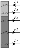
Figure 4: Schematic representation of the 5-quark component of baryon wavefunctions. The light gray rectangle stands for the pair wavefunction $W^{j_{i}\sigma_{i}}_{j_{k}\sigma_{k}}(\mathbf{p}_{i},\mathbf{p}_{k})$ where the reversed arrow represents the antiquark.

8 5-quark components of baryons

The 5-quark component of the baryon wavefunctions is obtained by expanding the coherent exponential (4) to the linear order in the $q\bar{q}$ pair. The projection involves now along with the three $R$’s from the discrete level two additional matrices $R\,R^{\dagger}$ that rotate the quark-antiquark pair in the $SU(3)$ space

$$T(B)^{f_{1}f_{2}f_{3}f_{4},j_{5}}_{j_{1}j_{2}j_{3}j_{4},f_{5},k}\equiv\int\mathrm{d}R\,B^{*}_{k}(R)R^{f_{1}}_{j_{1}}R^{f_{2}}_{j_{2}}R^{f_{3}}_{j_{3}}R^{f_{4}}_{j_{4}}R^{{\dagger}j_{5}}_{f_{5}}.$$ (38)

One then obtain the following 5-quark component of the neutron wavefunction in the momentum space

$$(|n\rangle_{k})^{f_{1}f_{2}f_{3}f_{4},\sigma_{1}\sigma_{2}\sigma_{3}\sigma_{4}}_{f_{5},\sigma_{5}}(\mathbf{p}_{1}\ldots\mathbf{p}_{5}) = \frac{\sqrt{8}}{360}\,F^{j_{1}\sigma_{1}}(\mathbf{p}_{1})F^{j_{2}\sigma_{2}}(\mathbf{p}_{2})F^{j_{3}\sigma_{3}}(\mathbf{p}_{3})W^{j_{4}\sigma_{4}}_{j_{5}\sigma_{5}}(\mathbf{p}_{4},\mathbf{p}_{5})$$ (39)

$$\times \epsilon_{k^{\prime}k}\left\{\epsilon^{f_{1}f_{2}}\epsilon_{j_{1}j_{2}}\left[\delta^{f_{3}}_{2}\delta^{f_{4}}_{f_{5}}\left(4\delta^{j_{5}}_{j_{4}}\delta^{k^{\prime}}_{j_{3}}-\delta^{j_{5}}_{j_{3}}\delta^{k^{\prime}}_{j_{4}}\right)+\delta^{f_{4}}_{2}\delta^{f_{3}}_{f_{5}}\left(4\delta^{j_{5}}_{j_{3}}\delta^{k^{\prime}}_{j_{4}}-\delta^{j_{5}}_{j_{4}}\delta^{k^{\prime}}_{j_{3}}\right)\right]\right.$$

$$+ \left.\epsilon^{f_{1}f_{4}}\epsilon_{j_{1}j_{4}}\left[\delta^{f_{2}}_{2}\delta^{f_{3}}_{f_{5}}\left(4\delta^{j_{5}}_{j_{3}}\delta^{k^{\prime}}_{j_{2}}-\delta^{j_{5}}_{j_{2}}\delta^{k^{\prime}}_{j_{3}}\right)+\delta^{f_{3}}_{2}\delta^{f_{2}}_{f_{5}}\left(4\delta^{j_{5}}_{j_{2}}\delta^{k^{\prime}}_{j_{3}}-\delta^{j_{5}}_{j_{3}}\delta^{k^{\prime}}_{j_{2}}\right)\right]\right\}$$

$$+ \textrm{permutations of 1,2,3}.$$

The color degrees of freedom are not explicitly written but the three valence quarks (1,2,3) are still antisymmetric in color while the quark-antiquark pair (4,5) is a color singlet. The wavefunction is schematically represented on Fig. 4.

Exotic baryons from the $\left({\bf\overline{10}},\frac{1}{2}^{+}\right)$ multiplet, despite the inexistence of a 3-quark component, have such a 5-quark component in their wavefunction. One has for example the following wavefunction for the $\Theta^{+}$

$$(|\Theta^{+}\rangle_{k})^{f_{1}f_{2}f_{3}f_{4},\sigma_{1}\sigma_{2}\sigma_{3}\sigma_{4}}_{f_{5},\sigma_{5}}(\mathbf{p}_{1}\ldots\mathbf{p}_{5}) = \frac{\sqrt{30}}{180}\,F^{j_{1}\sigma_{1}}(\mathbf{p}_{1})F^{j_{2}\sigma_{2}}(\mathbf{p}_{2})F^{j_{3}\sigma_{3}}(\mathbf{p}_{3})W^{j_{4}\sigma_{4}}_{j_{5}\sigma_{5}}(\mathbf{p}_{4},\mathbf{p}_{5})$$ (40)

$$\times \epsilon^{f_{1}f_{2}}\epsilon^{f_{3}f_{4}}\epsilon_{j_{1}j_{2}}\epsilon_{j_{3}j_{4}}\delta^{3}_{f_{5}}\delta^{j_{5}}_{k}$$

$$+ \textrm{ permutations of 1,2,3}.$$

The color structure is here very simple: $\epsilon^{\alpha_{1}\alpha_{2}\alpha_{3}}\delta^{\alpha_{4}}_{\alpha_{5}}$. This wavefunction says that we have two $ud$ pairs in the spin- and isospin-zero combination and that the whole $\Theta^{+}$ spin is carried by the $\bar{s}$ quark. One has naturally obtained the minimal quark content of the $\Theta^{+}$ pentaquark $uudd\bar{s}$.

9 Normalizations, vector and axial charges

The normalization of a Fock component $n$ of a specific spin-$\frac{1}{2}$ baryon $B$ wavefunction is obtained by

$$\mathcal{N}^{(n)}(B)=\frac{1}{2}\,\delta^{k}_{l}\langle\Psi^{(n)l}(B)|\Psi^{(n)}_{k}(B)\rangle.$$ (41)

One has to drag all annihilation operators in $\Psi^{(n){\dagger}l}(B)$ to the right and the creation operators in $\Psi^{(n)}_{k}(B)$ to the left so that the vacuum state $|\Omega_{0}\rangle$ is nullified. One then gets a non-zero result due to the anticommutation relations (27) or equivalently to the “contractions” of the operators.

A typical physical observable is the matrix element of some operator (preferably written in terms of quark annihilation-creation operators $a$, $b$, $a^{\dagger}$, $b^{\dagger}$) sandwiched between the initial and final baryon wavefunctions. As Diakonov and Petrov did in their paper [11], we shall consider only the operators of the vector and axial charges which can be written as

$$\left\{\begin{array}[]{c}Q\\ Q_{5}\end{array}\right\}=\int\mathrm{d}^{3}\mathbf{x}\,\bar{\psi}_{e}J^{e}_{h}\left\{\begin{array}[]{c}\gamma_{0}\\ \gamma_{0}\gamma_{5}\end{array}\right\}\psi^{h} = \int\mathrm{d}z\,\frac{\mathrm{d}^{2}\mathbf{p}_{\perp}}{(2\pi)^{2}}\left[a^{\dagger}_{e\pi}(z,\mathbf{p}_{\perp})a^{h\rho}(z,\mathbf{p}_{\perp})J^{e}_{h}\left\{\begin{array}[]{c}\delta^{\pi}_{\rho}\\ (-\sigma_{3})^{\pi}_{\rho}\end{array}\right\}\right.$$ (48)

$$- \left.b^{{\dagger}h\rho}(z,\mathbf{p}_{\perp})b_{e\pi}(z,\mathbf{p}_{\perp})J^{e}_{h}\left\{\begin{array}[]{c}\delta^{\pi}_{\rho}\\ (-\sigma_{3})^{\pi}_{\rho}\end{array}\right\}\right]$$ (51)

where $J^{e}_{h}$ is the flavor content of the charge and $\pi,\rho=1,2=L,R$ are helicity states. Notice that there are neither $a^{\dagger}b^{\dagger}$ nor $ab$ terms in the charges. This is a great advantage of the IMF where the number of $q\bar{q}$ pairs is not changed by the current. Hence there will only be diagonal transitions in the Fock space, i.e. the charges can be decomposed into the sum of the contributions from all Fock components $Q=\sum_{n}Q^{(n)}$, $Q_{5}=\sum_{n}Q^{(n)}_{5}$. Notice that there is also a color index which is just summed up.

The axial charges of the nucleon are defined as forward matrix elements of the axial current

$$\langle N(p)|\bar{\psi}\gamma_{\mu}\gamma_{5}\lambda^{a}\psi|N(p)\rangle=g^{(a)}_{A}\bar{u}(p)\gamma_{\mu}\gamma_{5}u(p)$$ (52)

where $a=0,3,8$ and $\lambda^{3},\lambda^{8}$ are Gell-Mann matrices, $\lambda^{0}$ is just in this context the $3\times 3$ unit matrix. These axial charges are related to the first moment of the polarized quark distributions

$$g^{(3)}_{A}=\Delta u-\Delta d,\qquad g^{(8)}_{A}=\frac{1}{\sqrt{3}}(\Delta u+\Delta d-2\Delta s),\qquad g^{(0)}_{A}=\Delta u+\Delta d+\Delta s$$ (53)

where $\Delta q\equiv\int_{0}^{1}\mathrm{d}z\left[q_{\uparrow}(z)-q_{\downarrow}(z)+\bar{q}_{\uparrow}(z)-\bar{q}_{\downarrow}(z)\right]$. Because of isospin symmetry, we expect that $g^{(3)}_{A}$ is the same as the axial charge obtained by the matrix element of the transition $p\to\pi^{+}n$.

9.1 3-quark contribution

If one looks to the 3-quark component of a baryon wavefunction, one can see that there are $3!$ possible and equivalent contractions of the annihilation-creation operators. The contraction in color then gives another factor of $3!=\epsilon^{\alpha_{1}\alpha_{2}\alpha_{3}}\epsilon_{\alpha_{1}\alpha_{2}\alpha_{3}}$. From eq. (34,41) on can express the normalization of the 3-quark component of baryon wavefunctions as

$$\mathcal{N}^{(3)}(B) = \frac{6\cdot 6}{2}\,\delta^{k}_{l}T(B)^{f_{1}f_{2}f_{3}}_{j_{1}j_{2}j_{3},k}T(B)_{f_{1}f_{2}f_{3}}^{l_{1}l_{2}l_{3},l}\int\mathrm{d}z_{1,2,3}\,\frac{\mathrm{d}^{2}\mathbf{p}_{1,2,3\perp}}{(2\pi)^{6}}\,\delta(z_{1}+z_{2}+z_{3}-1)(2\pi)^{2}\delta^{(2)}(\mathbf{p}_{1\perp}+\mathbf{p}_{2\perp}+\mathbf{p}_{3\perp})$$ (54)

$$\times F^{j_{1}\sigma_{1}}(p_{1})F^{j_{2}\sigma_{2}}(p_{2})F^{j_{3}\sigma_{3}}(p_{3})F^{\dagger}_{l_{1}\sigma_{1}}(p_{1})F^{\dagger}_{l_{2}\sigma_{2}}(p_{2})F^{\dagger}_{l_{3}\sigma_{3}}(p_{3})$$

where $F^{j\sigma}(p)\equiv F^{j\sigma}(z,\mathbf{p}_{\perp})$ are the discrete-level wavefunctions (31,32). In the non-relativistic limit, one can write $F^{j\sigma}(p)F^{\dagger}_{l\sigma}(p)\approx\delta^{j}_{l}h^{2}(p)$ (see eq. (33)). This 3-quark normalization is schematically represented in Fig. 6.

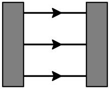
Figure 5: Schematic representation of the 3-quark normalization. All contractions of the annihilation-creation operators are equivalent to this specific one. Each quark line stands for the color, flavor and spin contractions $\delta^{\alpha_{i}}_{\alpha^{\prime}_{i}}\delta^{f_{i}}_{f^{\prime}_{i}}\delta^{\sigma_{i}}_{\sigma^{\prime}_{i}}\int\mathrm{d}z^{\prime}_{i}\,\mathrm{d}^{2}\mathbf{p}^{\prime}_{i\perp}\delta(z_{i}-z^{\prime}_{i})\delta^{(2)}(\mathbf{p}_{i\perp}-\mathbf{p}^{\prime}_{i\perp})$.

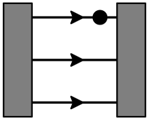
Figure 6: Schematic representation of the 3-quark contribution to a charge. The black dot stands for the one-quark operator with flavor content $J^{e}_{h}$. Since all three quark lines are equivalent one has three times this specific contribution.

In the 3-quark sector, there is no antiquark which means that the $b^{\dagger}b$ part of the current does not play. As in the 3-quark normalization one gets the factor $6\cdot 6$ from all contractions. Let the third quark be the one whose charge is measured. One then obtains an additional factor of 3 from the three quarks to which the charge operator can be applied (see Fig. 6). If we denote by $\int(\mathrm{d}p_{1-3})$ the integrals over momenta with the conservation $\delta$-functions as in eq. (54) one obtains the following expression for matrix element of the vector charge

$$V^{(3)}(1\to 2) = \frac{6\cdot 6\cdot 3}{2}\,\delta^{k}_{l}T(1)^{f_{1}f_{2}f_{3}}_{j_{1}j_{2}j_{3},k}T(2)_{f_{1}f_{2}g_{3}}^{l_{1}l_{2}l_{3},l}\int(\mathrm{d}p_{1-3})$$ (55)

$$\times \Big{[}F^{j_{1}\sigma_{1}}(p_{1})F^{j_{2}\sigma_{2}}(p_{2})F^{j_{3}\sigma_{3}}(p_{3})\Big{]}\left[F^{\dagger}_{l_{1}\sigma_{1}}(p_{1})F^{\dagger}_{l_{2}\sigma_{2}}(p_{2})F^{\dagger}_{l_{3}\tau_{3}}(p_{3})\right]\left[\delta^{\tau_{3}}_{\sigma_{3}}J^{g_{3}}_{f_{3}}\right].$$

We consider here for simplicity only matrix elements with zero momentum transfer.

The axial charge is easily obtained from the vector one. One just has to replace the averaging over baryon spin by $\frac{1}{2}(-\sigma_{3})^{k}_{l}$ and the axial charge operator involves now $(-\sigma_{3})^{\tau_{3}}_{\sigma_{3}}$ instead of $\delta^{\tau_{3}}_{\sigma_{3}}$. One then has

$$A^{(3)}(1\to 2) = \frac{6\cdot 6\cdot 3}{2}\,(-\sigma_{3})^{k}_{l}T(1)^{f_{1}f_{2}f_{3}}_{j_{1}j_{2}j_{3},k}T(2)_{f_{1}f_{2}g_{3}}^{l_{1}l_{2}l_{3},l}\int(\mathrm{d}p_{1-3})$$ (56)

$$\times \Big{[}F^{j_{1}\sigma_{1}}(p_{1})F^{j_{2}\sigma_{2}}(p_{2})F^{j_{3}\sigma_{3}}(p_{3})\Big{]}\left[F^{\dagger}_{l_{1}\sigma_{1}}(p_{1})F^{\dagger}_{l_{2}\sigma_{2}}(p_{2})F^{\dagger}_{l_{3}\tau_{3}}(p_{3})\right]\left[(-\sigma_{3})^{\tau_{3}}_{\sigma_{3}}J^{g_{3}}_{f_{3}}\right].$$

9.2 5-quark contributions

In the 5-quark component of the baryon wavefunctions there are already two types of contributions to the normalization: the direct and the exchange ones (see Fig. 7).

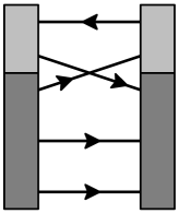
Figure 7: Schematic representation of the 5-quark direct (left) and exchange (right) contributions to the normalization.

In the former, one contracts the $a^{\dagger}$ from the pair wavefunction with the $a$ in the conjugate pair and all the valence operators are contracted with each other. As in the 3-quark normalization, there are 6 equivalent possibilities but the contractions in color give now a factor of $6\cdot 3=\epsilon^{\alpha_{1}\alpha_{2}\alpha_{3}}\epsilon_{\alpha_{1}\alpha_{2}\alpha_{3}}\delta^{\alpha}_{\alpha}$ because of the sum over color in the pair, then giving a total factor of 108. In the exchange contribution, one contracts the $a^{\dagger}$ from the pair with one of the three $a$’s from the conjugate discrete level. Vice versa, the $a$ from the conjugate pair is contracted with one of the three $a^{\dagger}$’s from the discrete level. There are at all 18 equivalent possibilities but the contractions in color give only a factor of $6=\epsilon^{\alpha_{1}\alpha_{2}\alpha}\epsilon_{\alpha_{1}\alpha_{2}\alpha_{3}}\delta^{\alpha_{3}}_{\alpha}$ and so one gets also a global factor of 108 for the exchange contribution but with an additional minus sign because one has to anticommute fermion operators to obtain exchange terms. We thus obtain the following expression for the 5-quark normalization

$$\mathcal{N}^{(5)}(B) = \frac{108}{2}\,\delta^{k}_{l}T(B)^{f_{1}f_{2}f_{3}f_{4},j_{5}}_{j_{1}j_{2}j_{3}j_{4},f_{5},k}T(B)_{f_{1}f_{2}g_{3}g_{4},l_{5}}^{l_{1}l_{2}l_{3}l_{4},f_{5},l}\int(\mathrm{d}p_{1-5})$$ (57)

$$\times F^{j_{1}\sigma_{1}}(p_{1})F^{j_{2}\sigma_{2}}(p_{2})F^{j_{3}\sigma_{3}}(p_{3})W^{j_{4}\sigma_{4}}_{j_{5}\sigma_{5}}(p_{4},p_{5})F^{\dagger}_{l_{1}\sigma_{1}}(p_{1})F^{\dagger}_{l_{2}\sigma_{2}}(p_{2})$$

$$\times \left[F^{\dagger}_{l_{3}\sigma_{3}}(p_{3})W_{c\,l_{4}\sigma_{4}}^{l_{5}\sigma_{5}}(p_{4},p_{5})\delta^{g_{3}}_{f_{3}}\delta^{g_{4}}_{f_{4}}-F^{\dagger}_{l_{3}\sigma_{4}}(p_{4})W_{c\,l_{4}\sigma_{3}}^{l_{5}\sigma_{5}}(p_{3},p_{5})\delta^{g_{3}}_{f_{4}}\delta^{g_{4}}_{f_{3}}\right]$$

where we have denoted

$$\int(\mathrm{d}p_{1-5})=\int\mathrm{d}z_{1-5}\,\delta(z_{1}+\ldots+z_{5}-1)\int\frac{\mathrm{d}^{2}\mathbf{p}_{1-5\perp}}{(2\pi)^{10}}\,(2\pi)^{2}\delta^{(2)}(\mathbf{p}_{1\perp}+\ldots+\mathbf{p}_{5\perp}).$$ (58)

These schematic representations or diagrams are really useful when one wishes to determine all the different possible contractions of annihilation-creation operators, the number of equivalent ones and their relative signs. In Appendix B we give some general rules that help one that desires to explore any specific Fock component of a baryon.

Concerning the vector and axial charges, we have three types of direct contributions and four types of exchange contributions.

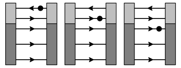
Figure 8: Schematic representation of the three type of 5-quark direct contributions to the charges.

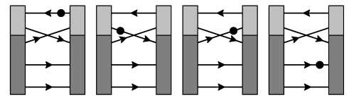
Figure 9: Schematic representation of the four types of 5-quark exchange contributions to the charges.

From schematic representations of these contributions (see Figs. 9,9), it is easy to write the direct and exchange transitions. We will write only vector charges since axial ones are obtained in the same way as in the 3-quark sector (the charge operator is in bold).

Direct contributions:

$$V^{(5)\textrm{direct}}(1\to 2) = \frac{108}{2}\,\delta^{k}_{l}T(1)^{f_{1}f_{2}f_{3}f_{4},j_{5}}_{j_{1}j_{2}j_{3}j_{4},f_{5},k}T(2)_{f_{1}f_{2}g_{3}g_{4},l_{5}}^{l_{1}l_{2}l_{3}l_{4},g_{5},l}\int(\mathrm{d}p_{1-5})$$ (59)

$$\times F^{j_{1}\sigma_{1}}(p_{1})F^{j_{2}\sigma_{2}}(p_{2})F^{j_{3}\sigma_{3}}(p_{3})W^{j_{4}\sigma_{4}}_{j_{5}\sigma_{5}}(p_{4},p_{5})F^{\dagger}_{l_{1}\sigma_{1}}(p_{1})F^{\dagger}_{l_{2}\sigma_{2}}(p_{2})F^{\dagger}_{l_{3}\tau_{3}}(p_{3})W_{c\,l_{4}\tau_{4}}^{l_{5}\tau_{5}}(p_{4},p_{5})$$

$$\times \left[-\delta^{g_{3}}_{f_{3}}\delta^{g_{4}}_{f_{4}}\boldsymbol{J^{f_{5}}_{g_{5}}}\delta^{\tau_{3}}_{\sigma_{3}}\delta^{\tau_{4}}_{\sigma_{4}}\boldsymbol{\delta_{\tau_{5}}^{\sigma_{5}}}+\delta^{g_{3}}_{f_{3}}\boldsymbol{J^{g_{4}}_{f_{4}}}\delta^{f_{5}}_{g_{5}}\delta^{\tau_{3}}_{\sigma_{3}}\boldsymbol{\delta^{\tau_{4}}_{\sigma_{4}}}\delta_{\tau_{5}}^{\sigma_{5}}+3\boldsymbol{J^{g_{3}}_{f_{3}}}\delta^{g_{4}}_{f_{4}}\delta^{f_{5}}_{g_{5}}\boldsymbol{\delta^{\tau_{3}}_{\sigma_{3}}}\delta^{\tau_{4}}_{\sigma_{4}}\delta_{\tau_{5}}^{\sigma_{5}}\right].$$

Exchange contributions:

$$V^{(5)\textrm{exchange}}(1\to 2) = -\frac{108}{2}\,\delta^{k}_{l}T(1)^{f_{1}f_{2}f_{3}f_{4},j_{5}}_{j_{1}j_{2}j_{3}j_{4},f_{5},k}T(2)_{f_{1}g_{2}g_{3}g_{4},l_{5}}^{l_{1}l_{2}l_{3}l_{4},g_{5},l}\int(\mathrm{d}p_{1-5})$$ (60)

$$\times F^{j_{1}\sigma_{1}}(p_{1})F^{j_{2}\sigma_{2}}(p_{2})F^{j_{3}\sigma_{3}}(p_{3})W^{j_{4}\sigma_{4}}_{j_{5}\sigma_{5}}(p_{4},p_{5})F^{\dagger}_{l_{1}\sigma_{1}}(p_{1})F^{\dagger}_{l_{2}\tau_{2}}(p_{2})F^{\dagger}_{l_{3}\tau_{3}}(p_{3})W_{c\,l_{4}\tau_{4}}^{l_{5}\tau_{5}}(p_{3},p_{5})$$

$$\times \left[-\delta^{g_{2}}_{f_{2}}\delta^{g_{4}}_{f_{3}}\delta^{g_{3}}_{f_{4}}\boldsymbol{J^{f_{5}}_{g_{5}}}\delta^{\tau_{2}}_{\sigma_{2}}\delta^{\tau_{4}}_{\sigma_{3}}\delta^{\tau_{3}}_{\sigma_{4}}\boldsymbol{\delta_{\tau_{5}}^{\sigma_{5}}}+\delta^{g_{2}}_{f_{2}}\delta^{g_{4}}_{f_{3}}\boldsymbol{J^{g_{3}}_{f_{4}}}\delta^{f_{5}}_{g_{5}}\delta^{\tau_{2}}_{\sigma_{2}}\delta^{\tau_{4}}_{\sigma_{3}}\boldsymbol{\delta^{\tau_{3}}_{\sigma_{4}}}\delta_{\tau_{5}}^{\sigma_{5}}\right.$$

$$+\left.\delta^{g_{2}}_{f_{2}}\boldsymbol{J^{g_{4}}_{f_{3}}}\delta^{g_{3}}_{f_{4}}\delta^{f_{5}}_{g_{5}}\delta^{\tau_{2}}_{\sigma_{2}}\boldsymbol{\delta^{\tau_{4}}_{\sigma_{3}}}\delta^{\tau_{3}}_{\sigma_{4}}\delta_{\tau_{5}}^{\sigma_{5}}+2\boldsymbol{J^{g_{2}}_{f_{2}}}\delta^{g_{4}}_{f_{3}}\delta^{g_{3}}_{f_{4}}\delta^{f_{5}}_{g_{5}}\boldsymbol{\delta^{\tau_{2}}_{\sigma_{2}}}\delta^{\tau_{4}}_{\sigma_{3}}\delta^{\tau_{3}}_{\sigma_{4}}\delta_{\tau_{5}}^{\sigma_{5}}\right].$$

We apply in the next sections these general formulae to compute the nucleon axial charges and estimate the $\Theta^{+}$ width.

10 Scalar overlap integrals in the IMF

The contractions in eqs. (57,59,60) are easily performed by Mathematica over all flavor $(f,g)$, isospin $(j,l)$ and spin $(\sigma,\tau)$ indices. One is then left with scalar integrals over longitudinal $z$ and transverse $\mathbf{p}_{\perp}$ momenta of the five quarks. The integrals over relative transverse momenta in the $q\bar{q}$ pair are generally UV divergent. This divergence should be cut by the momentum-dependent dynamical quark mass $M(p)$ (see eq. (1)). Following the authors of [9] we shall mimic the fall-off of $M(p)$ by the Pauli-Villars cutoff at $M_{\textrm{PV}}=556.8$ MeV (this value being chosen from the requirement that the pion decay constant $F_{\pi}=93$ MeV is reproduced from $M(0)=345$ MeV).

The pair wavefunction (25) is given in terms of the Fourier transforms of the mean chiral field $\Pi(\mathbf{q})$ and $\Sigma(\mathbf{q})$ (24). One has

$$\Pi(\mathbf{q})^{j}_{j^{\prime}}=i\frac{(q^{a}\tau^{a})^{j}_{j^{\prime}}}{|\mathbf{q}|}\,\Pi(q),\qquad\Pi(q)=\frac{4\pi}{q^{2}}\int_{0}^{\infty}\mathrm{d}r\,\sin P(r)(qr\cos qr-\sin qr)<0,$$ (61)

$$\Sigma(\mathbf{q})^{j}_{j^{\prime}}=\delta^{j}_{j^{\prime}}\Sigma(q),\qquad\Sigma(q)=\frac{4\pi}{q}\int_{0}^{\infty}\mathrm{d}r\,r(\cos P(r)-1)\sin qr<0.$$ (62)

We remind that $\mathbf{q}$ is the 3-momentum of the $q\bar{q}$ pair which is $\mathbf{q}=((\mathbf{p}+\mathbf{p}^{\prime})_{\perp},(z+z^{\prime})\mathcal{M})$.

10.1 5-quark direct integrals (old result)

Diakonov and Petrov have derived and computed the 5-quark direct integrals. There are four of them where the quark-loop integrands have to be understood as renormalized by the Pauli-Villars prescription $G(y,\mathcal{Q},\mathbf{q},M)-(M\to M_{\textrm{PV}})$

$$K_{\pi\pi} = \frac{M^{2}}{2\pi}\int\frac{\mathrm{d}^{3}\mathbf{q}}{(2\pi)^{3}}\,\Phi\left(\frac{q_{z}}{\mathcal{M}},\mathbf{q}_{\perp}\right)\theta(q_{z})q_{z}\Pi^{2}(\mathbf{q})\int^{1}_{0}\mathrm{d}y\int\frac{\mathrm{d}^{2}\mathcal{Q}_{\perp}}{(2\pi)^{2}}\frac{\mathcal{Q}^{2}_{\perp}+M^{2}}{(\mathcal{Q}^{2}_{\perp}+M^{2}+y(1-y)\mathbf{q}^{2})^{2}},$$ (63)

$$K_{\sigma\sigma} = \frac{M^{2}}{2\pi}\int\frac{\mathrm{d}^{3}\mathbf{q}}{(2\pi)^{3}}\,\Phi\left(\frac{q_{z}}{\mathcal{M}},\mathbf{q}_{\perp}\right)\theta(q_{z})q_{z}\Sigma^{2}(\mathbf{q})\int^{1}_{0}\mathrm{d}y\int\frac{\mathrm{d}^{2}\mathcal{Q}_{\perp}}{(2\pi)^{2}}\frac{\mathcal{Q}^{2}_{\perp}+M^{2}(2y-1)^{2}}{(\mathcal{Q}^{2}_{\perp}+M^{2}+y(1-y)\mathbf{q}^{2})^{2}},$$ (64)

$$K_{33} = \frac{M^{2}}{2\pi}\int\frac{\mathrm{d}^{3}\mathbf{q}}{(2\pi)^{3}}\,\Phi\left(\frac{q_{z}}{\mathcal{M}},\mathbf{q}_{\perp}\right)\theta(q_{z})\frac{q_{z}^{3}}{\mathbf{q}^{2}}\Pi^{2}(\mathbf{q})\int^{1}_{0}\mathrm{d}y\int\frac{\mathrm{d}^{2}\mathcal{Q}_{\perp}}{(2\pi)^{2}}\frac{\mathcal{Q}^{2}_{\perp}+M^{2}}{(\mathcal{Q}^{2}_{\perp}+M^{2}+y(1-y)\mathbf{q}^{2})^{2}},$$ (65)

$$K_{3\sigma} = \frac{M^{2}}{2\pi}\int\frac{\mathrm{d}^{3}\mathbf{q}}{(2\pi)^{3}}\,\Phi\left(\frac{q_{z}}{\mathcal{M}},\mathbf{q}_{\perp}\right)\theta(q_{z})\frac{q_{z}^{2}}{|\mathbf{q}|}\Pi(\mathbf{q})\Sigma(\mathbf{q})\int^{1}_{0}\mathrm{d}y\int\frac{\mathrm{d}^{2}\mathcal{Q}_{\perp}}{(2\pi)^{2}}\frac{\mathcal{Q}^{2}_{\perp}+M^{2}(2y-1)}{(\mathcal{Q}^{2}_{\perp}+M^{2}+y(1-y)\mathbf{q}^{2})^{2}}.$$ (66)

The authors have used the following variables

$$y=\frac{z^{\prime}}{z+z^{\prime}},\qquad\mathcal{Q}_{\perp}=\frac{z\mathbf{p}^{\prime}_{\perp}-z^{\prime}\mathbf{p}_{\perp}}{z+z^{\prime}}.$$ (67)

This set of variables allows one to first integrate over the relative momenta inside the $q\bar{q}$ pair $y$, $\mathcal{Q}_{\perp}$ and then over the 3-momentum $\mathbf{q}$ of the pair as a whole. The step function $\theta(q_{z})$ ensures that the longitudinal momentum carried by the pair is positive in the IMF. $\Phi(z,\mathbf{q}_{\perp})$ stands for the probability that three valence quarks “leave” the longitudinal fraction $z=z_{4}+z_{5}=q_{z}/\mathcal{M}$ and the transverse momentum $\mathbf{q}_{\perp}=\mathbf{p}_{4\perp}+\mathbf{p}_{5\perp}$ to the $q\bar{q}$ pair. In the non-relativistic limit, one has

$$\Phi(z,\mathbf{q}_{\perp})=\int\mathrm{d}z_{1,2,3}\frac{\mathrm{d}^{2}\mathbf{p}_{1,2,3\perp}}{(2\pi)^{6}}\,\delta(z+z_{1}+z_{2}+z_{3}-1)(2\pi)^{2}\delta^{(2)}(\mathbf{q}_{\perp}+\mathbf{p}_{1\perp}+\mathbf{p}_{2\perp}+\mathbf{p}_{3\perp})h^{2}(p_{1})h^{2}(p_{2})h^{2}(p_{3}).$$ (68)

Since in the 3-quark component of baryons there is no additional $q\bar{q}$ pair, all non-relativistic quantities in this sector are proportional to $\Phi(0,0)$. The normalization of the discrete-level wavefunction $h(p)$ being arbitrary, we choose it such that $\Phi(0,0)=1$.

10.2 Relativistic corrections to the discrete-level wavefunction (new result)

As quoted in [11] the uncertainty associated to the non-relativistic approximation is expected to be large. Indeed, they have systematically used the first-order perturbation theory in $1-\epsilon$ where $\epsilon=E_{\textrm{lev}}/M\sim 0.58$. They have thus

• ignored the lower component of the valence wavefunction $j(r)$

• ignored the distortion of the valence wavefunction by the sea (see eq. (32))

• used the approximate expression for the pair wavefunction (see eq. (25))

• neglected the 5-quark exchange diagrams when evaluating the 5-quark normalization and transition matrix elements

• neglected the 7-, 9-, …quark components in baryons.

There are three hints that this non-relativistic approximation is not satisfactory: first the actual expansion parameter $1-\epsilon=0.42$ is poor and second the ratio of the 5- to 3-quark normalization is 50%. Finally this can also be seen from the actual components $h(r)$ and $j(r)$ of the discrete-level wavefunction (Fig. 2). Diakonov and Petrov commented that the lower component $j(r)$ is “substantially” smaller than the upper one $h(r)$. In fact the $j(r)$ contribution to the normalization of the discrete-level wavefunction $\psi_{\textrm{lev}}(\mathbf{x})$ is still 20% (result in accordance with [27]). This combined with combinatorics factors in eq. (69) shows that considering the lower component $j(r)$ can have a big impact on the estimations. The nucleon is thus definitely a relativistic system.

We have improved the technique by considering the full expression for the discrete-level wavefunction (31). We have found that we have to use in the probability distribution (68) instead of $h^{2}(p_{1})h^{2}(p_{2})h^{2}(p_{3})$ the following combination

$$h^{2}(p_{1})h^{2}(p_{2})h^{2}(p_{3})+6h^{2}(p_{1})h^{2}(p_{2})\left[h(p_{3})\frac{p_{3z}}{|\mathbf{p}_{3}|}j(p_{3})\right]+3h^{2}(p_{1})h^{2}(p_{2})j^{2}(p_{3})$$

$$+12h^{2}(p_{1})\left[h(p_{2})\frac{p_{2z}}{|\mathbf{p}_{2}|}j(p_{2})\right]\left[h(p_{3})\frac{p_{3z}}{|\mathbf{p}_{3}|}j(p_{3})\right]+12h^{2}(p_{1})\left[h(p_{2})\frac{p_{2z}}{|\mathbf{p}_{2}|}j(p_{2})\right]j^{2}(p_{3})$$

$$+8\left[h(p_{1})\frac{p_{1z}}{|\mathbf{p}_{1}|}j(p_{1})\right]\left[h(p_{2})\frac{p_{2z}}{|\mathbf{p}_{2}|}j(p_{2})\right]\left[h(p_{3})\frac{p_{3z}}{|\mathbf{p}_{3}|}j(p_{3})\right]+3h^{2}(p_{1})j^{2}(p_{2})j^{2}(p_{3})$$

$$+12\left[h(p_{1})\frac{p_{1z}}{|\mathbf{p}_{1}|}j(p_{1})\right]\left[h(p_{2})\frac{p_{2z}}{|\mathbf{p}_{2}|}j(p_{2})\right]j^{2}(p_{3})+6\left[h(p_{1})\frac{p_{1z}}{|\mathbf{p}_{1}|}j(p_{1})\right]j^{2}(p_{2})j^{2}(p_{3})+j^{2}(p_{1})j^{2}(p_{2})j^{2}(p_{3})$$ (69)

where of course $p_{iz}=z_{i}\mathcal{M}-E_{\textrm{lev}}$. When an axial operator acts on the valence quarks it sees a slightly different probability distribution (this integral will be denoted by $\Psi(z,\mathbf{q}_{\perp})$)

$$h^{2}(p_{1})h^{2}(p_{2})h^{2}(p_{3})+6h^{2}(p_{1})h^{2}(p_{2})\left[h(p_{3})\frac{p_{3z}}{|\mathbf{p}_{3}|}j(p_{3})\right]+h^{2}(p_{1})h^{2}(p_{2})\frac{2p_{3z}^{2}+p_{3}^{2}}{p_{3}^{2}}j^{2}(p_{3})$$

$$+12h^{2}(p_{1})\left[h(p_{2})\frac{p_{2z}}{|\mathbf{p}_{2}|}j(p_{2})\right]\left[h(p_{3})\frac{p_{3z}}{|\mathbf{p}_{3}|}j(p_{3})\right]+4h^{2}(p_{1})\left[h(p_{2})\frac{p_{2z}}{|\mathbf{p}_{2}|}j(p_{2})\right]\frac{2p_{3z}^{2}+p_{3}^{2}}{p_{3}^{2}}j^{2}(p_{3})$$

$$+8\left[h(p_{1})\frac{p_{1z}}{|\mathbf{p}_{1}|}j(p_{1})\right]\left[h(p_{2})\frac{p_{2z}}{|\mathbf{p}_{2}|}j(p_{2})\right]\left[h(p_{3})\frac{p_{3z}}{|\mathbf{p}_{3}|}j(p_{3})\right]+h^{2}(p_{1})j^{2}(p_{2})\frac{4p_{3z}^{2}-p_{3}^{2}}{p_{3}^{2}}j^{2}(p_{3})$$

$$+4\left[h(p_{1})\frac{p_{1z}}{|\mathbf{p}_{1}|}j(p_{1})\right]\left[h(p_{2})\frac{p_{2z}}{|\mathbf{p}_{2}|}j(p_{2})\right]\frac{2p_{3z}^{2}+p_{3}^{2}}{p_{3}^{2}}j^{2}(p_{3})+2\left[h(p_{1})\frac{p_{1z}}{|\mathbf{p}_{1}|}j(p_{1})\right]j^{2}(p_{2})\frac{4p_{3z}^{2}-p_{3}^{2}}{p_{3}^{2}}j^{2}(p_{3})$$

$$+j^{2}(p_{1})j^{2}(p_{2})\frac{2p_{3z}^{2}-p_{3}^{2}}{p_{3}^{2}}j^{2}(p_{3}).$$ (70)

This distribution has been normalized in such a way that the prefactor of the axial charge is the same as the one of the vector charge (59).

Then in the 3-quark component of baryons all quantities are proportional to either $\Phi(0,0)$ or $\Psi(0,0)$. The normalization of the discrete-level wavefunctions $h(p)$ and $j(p)$ being arbitrary, we choose it such that $\Phi(0,0)=1$.

Note that we still haven’t taken into account the distortion of the valence level due to the sea.

10.3 5-quark exchange integrals (new result)

Our other improvement of the technique is the consideration of the exchange diagrams which were believed to have a strong impact on observables because of their sign opposite to the direct one [11] (see for example eq. (57)). We have found that for the exchange contributions there were thirteen non-zero scalar integrals. Since the quark from the sea is exchanged with a valence quark, we cannot disentangle the quark-antiquark pair from the valence quarks. At best two valence quarks can be factorized out and leave 9-dimensional integrals

$$K=\frac{M^{2}}{2\pi}\int(\mathrm{d}p_{3,4,5})\,\phi\left(\mathcal{Z},\mathbf{P}_{\perp}\right)\frac{\mathcal{M}^{2}}{2\pi Z^{\prime}Z}\,I(z_{3,4,5},\mathbf{p}_{3,4,5\perp})h(p_{3})h(p_{4}),$$ (71)

where $\mathcal{Z}=z_{3}+z_{4}+z_{5}$, $\mathbf{P}_{\perp}=(\mathbf{p}_{3}+\mathbf{p}_{4}+\mathbf{p}_{5})_{\perp}$, $Z$ is given by eq. (26) with $z=z_{4}$ and $z^{\prime}=z_{5}$ while $Z^{\prime}$ is the same but with the replacement $z_{4}\to z_{3}$. The function $I(z_{3,4,5},\mathbf{p}_{3,4,5\perp})$ stands for the thirteen integrands

$$I_{1} = \Sigma(\mathbf{q}^{\prime})\Sigma(\mathbf{q})\left(\mathbf{Q}^{\prime}_{\perp}\cdot\mathbf{Q}_{\perp}+M^{2}(z_{5}-z_{3})(z_{5}-z_{4})\right),$$ (72)

$$I_{2} = \Pi(\mathbf{q}^{\prime})\Pi(\mathbf{q})\,\frac{q^{\prime}\cdot q}{q^{\prime}q}\left(\mathbf{Q}^{\prime}_{\perp}\cdot\mathbf{Q}_{\perp}+M^{2}(z_{5}+z_{3})(z_{5}+z_{4})\right),$$ (73)

$$I_{3} = \Pi(\mathbf{q}^{\prime})\Pi(\mathbf{q})\,\frac{\mathbf{q}^{\prime}_{\perp}\times\mathbf{q}_{\perp}}{q^{\prime}q}\,(\mathbf{Q}^{\prime}_{\perp}\times\mathbf{Q}_{\perp}),$$ (74)

$$I_{4} = \Pi(\mathbf{q}^{\prime})\Pi(\mathbf{q})\,\frac{M(\mathbf{q}^{\prime}_{\perp}q_{z}-\mathbf{q}_{\perp}q^{\prime}_{z})}{q^{\prime}q}\cdot\left(\mathbf{Q}_{\perp}-\mathbf{Q}^{\prime}_{\perp}\right),$$ (75)

$$I_{5} = \Pi(\mathbf{q}^{\prime})\Pi(\mathbf{q})\,\frac{q^{\prime}_{z}q_{z}}{q^{\prime}q}\left(\mathbf{Q}^{\prime}_{\perp}\cdot\mathbf{Q}_{\perp}+M^{2}(z_{5}+z_{3})(z_{5}+z_{4})\right),$$ (76)

$$I_{6} = \Sigma(\mathbf{q}^{\prime})\Pi(\mathbf{q})\,\frac{q_{z}}{q}\left(\mathbf{Q}^{\prime}_{\perp}\cdot\mathbf{Q}_{\perp}+M^{2}(z_{5}-z_{3})(z_{5}+z_{4})\right),$$ (77)

$$I_{7} = \Sigma(\mathbf{q}^{\prime})\Pi(\mathbf{q})\,\frac{M\mathbf{q}_{\perp}}{q}\cdot\left(\mathbf{Q}^{\prime}_{\perp}(z_{5}+z_{4})-\mathbf{Q}_{\perp}(z_{5}-z_{3})\right),$$ (78)

$$I_{8} = \Sigma(\mathbf{q}^{\prime})\Sigma(\mathbf{q})\left(\mathbf{Q}^{\prime}_{\perp}\cdot\mathbf{Q}_{\perp}-M^{2}(z_{5}-z_{3})(z_{5}-z_{4})\right),$$ (79)

$$I_{9} = \Pi(\mathbf{q}^{\prime})\Pi(\mathbf{q})\,\frac{q^{\prime}\cdot q}{q^{\prime}q}\left(\mathbf{Q}^{\prime}_{\perp}\cdot\mathbf{Q}_{\perp}-M^{2}(z_{5}+z_{3})(z_{5}+z_{4})\right),$$ (80)

$$I_{10} = \Pi(\mathbf{q}^{\prime})\Pi(\mathbf{q})\,\frac{M(\mathbf{q}^{\prime}_{\perp}q_{z}+\mathbf{q}_{\perp}q^{\prime}_{z})}{q^{\prime}q}\cdot\left(\mathbf{Q}_{\perp}+\mathbf{Q}^{\prime}_{\perp}\right),$$ (81)

$$I_{11} = \Pi(\mathbf{q}^{\prime})\Pi(\mathbf{q})\,\frac{q^{\prime}_{z}q_{z}}{q^{\prime}q}\left(\mathbf{Q}^{\prime}_{\perp}\cdot\mathbf{Q}_{\perp}-M^{2}(z_{5}+z_{3})(z_{5}+z_{4})\right),$$ (82)

$$I_{12} = \Sigma(\mathbf{q}^{\prime})\Pi(\mathbf{q})\,\frac{q_{z}}{q}\left(\mathbf{Q}^{\prime}_{\perp}\cdot\mathbf{Q}_{\perp}-M^{2}(z_{5}-z_{3})(z_{5}+z_{4})\right),$$ (83)

$$I_{13} = \Sigma(\mathbf{q}^{\prime})\Pi(\mathbf{q})\,\frac{M\mathbf{q}_{\perp}}{q}\cdot\left(\mathbf{Q}^{\prime}_{\perp}(z_{5}+z_{4})+\mathbf{Q}_{\perp}(z_{5}-z_{3})\right),$$ (84)

where $\mathbf{q}=((\mathbf{p}_{4}+\mathbf{p}_{5})_{\perp},(z_{4}+z_{5})\mathcal{M})$ and $\mathbf{Q}_{\perp}=z_{4}\mathbf{p}_{5\perp}-z_{5}\mathbf{p}_{4\perp}$. The primed variables stand for the same as the unprimed ones but with the replacement $z_{4}\to z_{3}$. The regularization of those integrals is done exactly in the same way as for the direct contributions.

The function $\phi(\mathcal{Z},\mathbf{P}_{\perp})$ stands for the probability that two valence quarks “leave” the longitudinal fraction $\mathcal{Z}=z_{3}+z_{4}+z_{5}$ and the transverse momentum $\mathbf{P}_{\perp}=\mathbf{p}_{3\perp}+\mathbf{p}_{4\perp}+\mathbf{p}_{5\perp}$ to the rest of the partons

$$\phi(\mathcal{Z},\mathbf{P}_{\perp})=\int\mathrm{d}z_{1,2}\frac{\mathrm{d}^{2}\mathbf{p}_{1,2\perp}}{(2\pi)^{4}}\,\delta(\mathcal{Z}+z_{1}+z_{2}-1)(2\pi)^{2}\delta^{(2)}(\mathbf{P}_{\perp}+\mathbf{p}_{1\perp}+\mathbf{p}_{2\perp})h^{2}(p_{1})h^{2}(p_{2}).$$ (85)

We have kept of course the same normalization of the discrete-level wavefunction $h(p)$ as in the direct contributions, i.e. such that $\Phi(0,0)=\int(\mathrm{d}p)\,\phi(z,\mathbf{p}_{\perp})h^{2}(p)=1$. Anticipating on the results, we haven’t considered relativistic corrections to this probability distribution since exchange contributions appear to be fairly negligible. Exchange contributions have then been computed only in the non-relativistic limit.

11 Results

All normalizations, vector and axial charges are linear combinations of (63)-(66) for the direct contributions and of (72)-(84) for the exchange ones.

11.1 Old results

In their paper [11], Diakonov and Petrov have obtained the following combinations

Nucleon normalization:

$$\mathcal{N}^{(3)}(N) = 9\,\Phi(0,0),$$ (86)

$$\mathcal{N}^{(5)\textrm{direct}}(N) = \frac{18}{5}\left(11K_{\pi\pi}+23K_{\sigma\sigma}\right).$$ (87)

Axial charge of the $p\to\pi^{+}n$ transition:

$$A^{(3)}(p\to\pi^{+}n) = 15\,\Phi(0,0),$$ (88)

$$A^{(5)\textrm{direct}}(p\to\pi^{+}n) = \frac{6}{25}\left(209K_{\pi\pi}+559K_{\sigma\sigma}-34K_{33}-356K_{3\sigma}\right).$$ (89)

$\Theta^{+}$ normalization:

$$\mathcal{N}^{(5)\textrm{direct}}(\Theta)=\frac{36}{5}\left(K_{\pi\pi}+K_{\sigma\sigma}\right).$$ (90)

Axial charge of the $\Theta^{+}\to K^{+}n$ transition:

$$A^{(5)\textrm{direct}}(\Theta^{+}\to K^{+}n)=\frac{6}{5}\sqrt{\frac{3}{5}}\left(-7K_{\pi\pi}-5K_{\sigma\sigma}+8K_{33}+28K_{3\sigma}\right).$$ (91)

11.2 New results

We have obtained the exchange combinations relative to these quantities. On the top of that we have computed the matrix elements of $\bar{q}\gamma_{0}\gamma_{5}q$ with $q=u,d,s$ for the nucleon in order to obtain the three nucleon axial charges (53).

Nucleon normalization:

$$\mathcal{N}^{(5)\textrm{exchange}}(N)=\frac{-12}{5}\left(9K_{1}+4K_{3}+4K_{4}-17K_{6}-17K_{7}\right).$$ (92)

Axial charge of the $p\to\pi^{+}n$ transition:

$$A^{(5)\textrm{exchange}}(p\to\pi^{+}n) = \frac{-2}{25}\left(557K_{1}+K_{2}+221K_{3}+192K_{4}-2K_{5}-908K_{6}-978K_{7}\right.$$ (93)

$$\left.+98K_{8}-50K_{9}+62K_{10}+124K_{11}-48K_{12}-100K_{13}\right).$$

Proton first moment of polarized quark distributions:

$$\Delta u^{(3)} = 12\,\Phi(0,0),$$ (94)

$$\Delta d^{(3)} = -3\,\Phi(0,0),$$ (95)

$$\Delta s^{(3)} = 0,$$ (96)

$$\Delta u^{(5)\textrm{direct}}(p) = \frac{18}{25}\left(41K_{\pi\pi}+151K_{\sigma\sigma}+14K_{33}-74K_{3\sigma}\right),$$ (97)

$$\Delta d^{(5)\textrm{direct}}(p) = \frac{12}{25}\left(-43K_{\pi\pi}-53K_{\sigma\sigma}+38K_{33}+67K_{3\sigma}\right),$$ (98)

$$\Delta s^{(5)\textrm{direct}}(p) = \frac{12}{25}\left(-11K_{\pi\pi}-K_{\sigma\sigma}+16K_{33}+14K_{3\sigma}\right),$$ (99)

$$\Delta u^{(5)\textrm{exchange}}(p) = \frac{-6}{25}\left(153K_{1}-K_{2}+49K_{3}+48K_{4}+2K_{5}-262K_{6}-232K_{7}\right.$$ (100)

$$\left.+32K_{8}+8K_{10}+16K_{11}-32K_{12}\right),$$

$$\Delta d^{(5)\textrm{exchange}}(p) = \frac{-4}{25}\left(-49K_{1}-2K_{2}-37K_{3}-24K_{4}+4K_{5}+61K_{6}+141K_{7}\right.$$ (101)

$$\left.-K_{8}+25K_{9}-19K_{10}-38K_{11}-24K_{12}+50K_{13}\right),$$

$$\Delta s^{(5)\textrm{exchange}}(p) = \frac{-2}{25}\left(14K_{1}-8K_{2}-13K_{3}-6K_{4}+16K_{5}-26K_{6}+54K_{7}\right.$$ (102)

$$\left.+11K_{8}+25K_{9}-16K_{10}-32K_{11}-36K_{12}+50K_{13}\right).$$

It is then easy to obtain the three axial charges. As expected by isospin symmetry the axial charge obtained by the $p\to\pi^{+}n$ transition is the same as $g_{A}^{(3)}$ in any of the 3- or 5-quark direct or exchange contributions

$$g^{(3)}_{A^{(3)}} = A^{(3)}(p\to\pi^{+}n),$$ (103)

$$g^{(8)}_{A^{(3)}} = 3\sqrt{3}\,\Phi(0,0),$$ (104)

$$g^{(0)}_{A^{(3)}} = 9\,\Phi(0,0),$$ (105)

$$g^{(3)}_{A^{(5)\textrm{direct}}} = A^{(5)\textrm{direct}}(p\to\pi^{+}n),$$ (106)

$$g^{(8)}_{A^{(5)\textrm{direct}}} = \frac{18\sqrt{3}}{25}\left(9K_{\pi\pi}+39K_{\sigma\sigma}+6K_{33}-16K_{3\sigma}\right),$$ (107)

$$g^{(0)}_{A^{(5)\textrm{direct}}} = \frac{18}{5}\left(K_{\pi\pi}+23K_{\sigma\sigma}+10K_{33}-4K_{3\sigma}\right),$$ (108)

$$g^{(3)}_{A^{(5)\textrm{exchange}}} = A^{(5)\textrm{exchange}}(p\to\pi^{+}n),$$ (109)

$$g^{(8)}_{A^{(5)\textrm{exchange}}} = \frac{-6\sqrt{3}}{25}\left(37K_{1}+K_{2}+11K_{3}+12K_{4}-2K_{5}-68K_{6}-58K_{7}\right.$$ (110)

$$\left.+8K_{8}+2K_{10}+4K_{11}-8K_{12}\right),$$

$$g^{(0)}_{A^{(5)\textrm{exchange}}} = \frac{-6}{5}\left(25K_{1}-K_{2}+4K_{3}+6K_{4}+2K_{5}-46K_{6}-24K_{7}\right.$$ (111)

$$\left.+7K_{8}+5K_{9}-2K_{10}-4K_{11}-12K_{12}+10K_{13}\right).$$

For the vector charge of the $p\to\pi^{+}n$ transition one gets exactly the same expression as the normalization of the contribution under consideration, which means that the vector charge is conserved in each Fock component separately and even in the direct and exchange sectors separately.

Here are our results for the $\Theta^{+}$ pentaquark

$\Theta^{+}$ normalization:

$$\mathcal{N}^{(5)\textrm{exchange}}(\Theta)=\frac{-12}{5}\left(K_{3}+K_{4}-2K_{6}-2K_{7}\right).$$ (112)

Axial charge of the $\Theta^{+}\to K^{+}n$ transition:

$$A^{(5)\textrm{exchange}}(\Theta^{+}\to K^{+}n) = \frac{-2}{5}\sqrt{\frac{3}{5}}\left(-7K_{1}+K_{2}-7K_{3}-3K_{4}-2K_{5}+4K_{6}+18K_{7}\right.$$ (113)

$$\left.-10K_{8}+10K_{9}-10K_{10}-20K_{11}+20K_{13}\right).$$

When relativistic effects are considered, the axial operator changes the structure of the probability distribution. One has then to replace $K_{\pi\pi}$, $K_{\sigma\sigma}$ and $K_{33}$ by $K_{\pi\pi}^{\prime}$, $K_{\sigma\sigma}^{\prime}$ and $K_{33}^{\prime}$, i.e. the same integrals but with $\Phi(z,\mathbf{q}_{\perp})$ (eq. (69)) replaced by $\Psi(z,\mathbf{q}_{\perp})$ (eq. (70)). Note that $K_{3\sigma}$ is not affected since this integral appears only when the axial operator acts on the pair.

The numerical value of these matrix elements has to be properly normalized as in the following example

$$g_{A}(\Theta\to KN)=\frac{A^{(5)\textrm{direct}}(\Theta^{+}\to K^{+}n)+A^{(5)\textrm{exchange}}(\Theta^{+}\to K^{+}n)}{\sqrt{\mathcal{N}^{(5)\textrm{direct}}(\Theta)+\mathcal{N}^{(5)\textrm{exchange}}(\Theta)}\sqrt{\mathcal{N}^{(3)}(N)+\mathcal{N}^{(5)\textrm{direct}}(N)+\mathcal{N}^{(5)\textrm{exchange}}(N)}}.$$ (114)

12 Numerical results

In the evaluation of the scalar integrals we have used the quark mass $M=345$ MeV, the self-consistent profile function (6), the Pauli-Villars mass $M_{\textrm{PV}}=556.8$ MeV for the regularization of (63)-(66), (72)-(84) and the baryon mass $\mathcal{M}=1207$ MeV as it follows for the “classical” mass in the mean field approximation [5]. The self-consistent scalar $\Sigma(\mathbf{q})$ and pseudoscalar $\Pi(\mathbf{q})$ fields are plotted in Fig. 11. The probability distributions $\phi(z,\mathbf{q}_{\perp})$ (85) and $\Phi(z,\mathbf{q}_{\perp})$ (68) that two or three valence quarks leave the fraction $z$ of the baryon momentum and the transverse momentum $\mathbf{q}_{\perp}$ are plotted in Fig. 11 in the non-relativistic limit and in Fig. 12 with relativistic corrections to the discrete-level wavefunction. By comparison one immediately sees that relativistic corrections shift the bump in the probability distributions to lower values of $z$ and smear it a little bit. When relativistic corrections to an axial charge are considered one has to use the $\Psi(z,\mathbf{q}_{\perp})$ probability distribution which is slightly different (see Fig. 12) from the relativistically corrected $\Phi(z,\mathbf{q}_{\perp})$. We remind that the normalization of the discrete-level wavefunctions $h(p)$ (and $j(p)$) is chosen such that we have $\Phi(0,0)=1$.

The numerical evaluation of the non-relativistic direct integrals (63)-(66) yields

$$K_{\pi\pi}=0.0624,\qquad K_{\sigma\sigma}=0.0284,\qquad K_{33}=0.0373,\qquad K_{3\sigma}=0.0334.$$ (115)

We have recalculated the integrals. The numerical precision is the reason why these numbers are slightly different from those given in [11].

The numerical evaluation of the direct integrals (63)-(66) with relativistic corrections to the discrete-level wavefunction yields

$$K_{\pi\pi}=0.0365,\qquad K_{\sigma\sigma}=0.0140,\qquad K_{33}=0.0197,\qquad K_{3\sigma}=0.0163.$$ (116)

As one can expect from the comparison between Fig. 11 and 12 relativistic corrections reduce strongly (about one half) the values of the scalar integrals.

Figure 10: The self-consistent pseudoscalar $-|\mathbf{q}|\Pi(\mathbf{q})$ (solid) and scalar $-|\mathbf{q}|\Sigma(\mathbf{q})$ (dashed) fields in baryons. The horizontal axis unit is $M$.

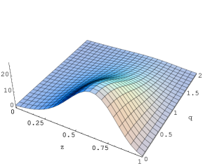
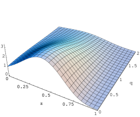
Figure 11: The non-relativistic probability distribution that two (left) or three (right) valence quarks leave the fraction $z$ of the baryon momentum and the transverse momentum $\mathbf{q}_{\perp}$ plotted in units of $M$ and normalized to unity for $z=\mathbf{q}_{\perp}=0$.

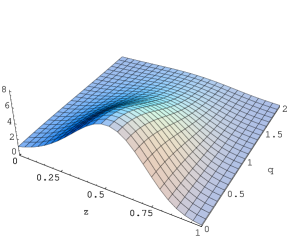
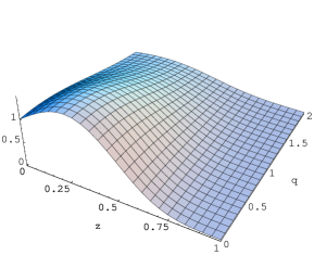
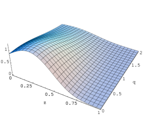
Figure 12: The probability distribution that two (left) or three (middle) valence quarks leave the fraction $z$ of the baryon momentum and the transverse momentum $\mathbf{q}_{\perp}$ with relativistic corrections to the discrete-level wavefunction plotted in units of $M$ and normalized to unity for $z=\mathbf{q}_{\perp}=0$. Relativistic corrections clearly shift the bump in the probability distributions to smaller values $z$ meaning that they leave less longitudinal momentum fraction to the quark-antiquark pair. They seem also to smear a little bit this bump. On the right is plotted the probability distribution that enters scalar integrals when an axial charge is considered.

The numerical evaluation of the direct integrals (63)-(66) with relativistic corrections to the discrete-level wavefunction that enter axial charges and first moment of polarized quark distributions yields

$$K_{\pi\pi}^{\prime}=0.0300,\qquad K_{\sigma\sigma}^{\prime}=0.0112,\qquad K_{33}^{\prime}=0.0163.$$ (117)

The numerical evaluation of the exchange integrals (72)-(84) yields

$$K_{1}=0.0056,\qquad K_{2}=0.0097,\qquad K_{3}=-0.0008\qquad K_{4}=0.0047,$$

$$K_{5}=0.0086,\qquad K_{6}=0.0042,\qquad K_{7}=0.0029,\qquad K_{8}=0.0043,\qquad K_{9}=0.0031,$$

$$K_{10}=0.0069,\qquad K_{11}=0.0017,\qquad K_{12}=0.0057,\qquad K_{13}=0.0023.$$ (118)

All nucleon axial charges and first moment of polarized quark distributions are collected and presented in Table 1.

Table 1: Results for the nucleon: axial charges, first moment of polarized quark distributions and ratio of the 5- to the 3-quark normalization. First, results in the non-relativistic approximation are given, then with relativistic corrections to the discrete-level wavefunction.

	Non-relativistic			Relativistic
	$3q$	$3q+5q$ direct	$3q+5q$ dir.+ exch.	$3q$	$3q+5q$ direct	Exp. value
$g^{(3)}_{A}$	5/3	1.359	1.360	1.435	1.241	1.257$\pm$0.003
$g^{(8)}_{A}$	$1/\sqrt{3}$	0.499	0.500	0.497	0.444	0.34$\pm$0.02
$g^{(0)}_{A}$	1	0.900	0.901	0.861	0.787	0.31$\pm$0.07
$\Delta u$	4/3	1.123	1.125	1.148	1.011	0.83$\pm$0.03
$\Delta d$	-1/3	-0.236	-0.235	-0.287	-0.230	-0.43$\pm$0.043
$\Delta s$	0	0.012	0.012	0	0.006	-0.10$\pm$0.03
$\mathcal{N}^{(5)}/\mathcal{N}^{(3)}$	–	0.536	0.550	–	0.289	–

Although the 5-quark contributions improve the too simplistic 3-quark view, one can see that the direct contributions are dominant while the exchange ones are clearly negligible. This is partly due to the small values of the integrals (118) which are phase-space suppressed compared to (115). One can also notice that relativistic corrections have a non-negligible impact on the observables (the relativistic correction to the 3-quark component of the axial charges amounts to a multiplication of the non-relativistic values by a factor of 0.861) and then conclude that the non-relativistic approximation is too crude. Since non-relativistic exchange contributions change the observable so little we haven’t computed their relativistic corrections.

We have fairly well reproduced $g^{(3)}_{A}=1.241$ while the experimental value is 1.257$\pm$0.003. However the computed axial charges $g^{(8)}_{A}$ and $g^{(0)}_{A}$ are not satisfactory (0.444 and 0.787 against 0.34$\pm$0.02 and 0.31$\pm$0.07). Only additional quark-antiquark pairs contribute to $\Delta s$. Unfortunately the effect of one pair in our computation is in the wrong direction since the contribution is positive. On the top of that relativistic effects and addition of a pair reduce the non-relativistic 3-quark amplitude of $\Delta d$ instead of increasing it. In order to preserve $g^{(3)}_{A}$, one should explain the shift of 0.2 between experimental and computed values for $\Delta u$ and $\Delta d$.

The axial charge of the $\Theta^{+}\to K^{+}n$ transition allows one to roughly estimate the $\Theta^{+}$ width. If we assume the approximate $SU(3)$ chiral symmetry one can obtain the $\Theta\to KN$ pseudoscalar coupling from the generalized Goldberger-Treiman relation

$$g_{\Theta KN}=\frac{g_{A}(\Theta\to KN)(M_{\Theta}+M_{N})}{2F_{K}}$$ (119)

where we use $M_{\Theta}=1530$ MeV, $M_{N}=940$ MeV and $F_{K}=1.2F_{\pi}=112$ MeV. Once this transition pseudoscalar constant is known one can evaluate the $\Theta^{+}$ width from the general expression for the $\frac{1}{2}^{+}$ hyperon decay [28]

$$\Gamma_{\Theta}=2\,\frac{g^{2}_{\Theta KN}|\mathbf{p}|}{8\pi}\frac{(M_{\Theta}-M_{N})^{2}-m_{K}^{2}}{M_{\Theta}^{2}}$$ (120)

where $|\mathbf{p}|=\sqrt{(M_{\Theta}^{2}-M_{N}^{2}-m_{K}^{2})^{2}-4M_{N}^{2}m_{K}^{2}}/2M_{\Theta}=254$ MeV is the kaon momentum in the decay ($m_{K}=495$ MeV) and the factor of 2 stands for the equal probability $K^{+}n$ and $K^{0}p$ decays. All results for the $\Theta^{+}$ pentaquark are collected in Table 2.

Table 2: Results for the $\Theta^{+}$ pentaquark: axial charge of the $\Theta^{+}\to K^{+}n$ transition, $\Theta\to KN$ pseudoscalar coupling and $\Theta^{+}$ width. First, results in the non-relativistic approximation are given, then with relativistic corrections to the discrete-level wavefunction.

	Non-relativistic		Relativistic
	$3q+5q$ direct	$3q+5q$ dir.+ exch.	$3q+5q$ direct
$g_{A}(\Theta\to KN)$	0.202	0.203	0.144
$g_{\Theta KN}$	2.230	2.242	1.592
$\Gamma_{\Theta}$ (MeV)	4.427	4.472	2.256

Such as in the nucleon case, the exchange contribution is negligible. However, relativistic corrections to the discrete-level wavefunction are not negligible (reduction of 30% for the axial coupling and of 50% for the width). This can be expected from the fact that the $\Theta^{+}$ width directly depends on the number of $q\bar{q}$ pairs in ordinary baryons [11]. Indeed, the axial transition from the $\Theta^{+}$ to a nucleon can only take place between similar Fock components. This means that the 5-quark component of the $\Theta^{+}$ can only be connected with the 5-quark component of the nucleon. Since relativistic corrections reduce the 5- to 3-quark normalization of the nucleon, so is the $\Theta^{+}$ width.

13 Conclusion

The Chiral Quark Soliton Model [4] provides a relativistic description of the light baryons with an indefinite number of $q\bar{q}$ pairs. Using this model, Diakonov and Petrov [11] have presented a technique allowing one to write down explicitly the 3-, 5-, 7-, …quark wavefunctions of the octet, decuplet and antidecuplet. It is important that the $q\bar{q}$ pair in the 5-quark component of any baryon is added in the form of a chiral field, which costs little energy. That is why the 5-quark component of the nucleon turns out to be substantial and why the exotic $\Theta^{+}$ baryon is expected to be light.

For self-consistency this technique has been reminded and then used in the present paper. It is really powerful and with sufficiently patience one can write any Fock component of any baryon and compute lots of matrix elements. Diakonov and Petrov have estimated the normalization of the 5-quark component of the nucleon as about 50% of the 3-quark component, meaning that about 1/3 of the time the nucleon is made of five quarks. They have also showed that the 5-quark component in the nucleon moves its axial charge $g_{A}(p\to\pi^{+}n)$ from the naive non-relativistic value 5/3 much closer to the experimental value. They have estimated the $\Theta^{+}$ width as being $\sim 4$ MeV thanks to the axial constant for the $\Theta\to KN$ transition and showed that it is proportional to the number of $q\bar{q}$ pairs in ordinary baryons. Assuming $SU(3)$ symmetry, the $\Theta^{+}$ width is additionally suppressed by the $SU(3)$ Clebsch-Gordan factors. Therefore, the $\Theta^{+}$ width of a few MeV appears naturally in the Chiral Quark Soliton Model without any parameter fixing.

However, these estimations are rather crude since several approximations were used (the first-order perturbation theory in $1-\epsilon$ where $\epsilon=E_{\textrm{lev}}/M\sim 0.58$): the lower component of the valence wavefunction $j(r)$ was ignored as well as the distortion of the valence wavefunction by the sea, an approximate expression for the pair wavefunction was used, the 7-, 9-, …quark components were neglected and exchange contributions to the 5-quark component were disregarded. It is difficult to evaluate the errors of these approximations. Unfortunately, the uncertainty associated with this non-relativistic approximation is expected to be large since the expansion parameter $1-\epsilon=0.42$ is poor. Another sign saying that the nucleon is a relativistic system comes from the 50% ratio of the 5-quark to the 3-quark normalization. It was also expected that exchange contributions reduce further the $\Theta^{+}$ width and that is what actually motivated the present work.

We have improved the technique by taking into account on the one hand the 5-quark exchange contributions and on the other hand relativistic corrections to the discrete-level wavefunction. Due to the relative sign of their contributions, the 5-quark exchange diagrams were expected to be a main source of error. In fact it turns out that they are completely negligible, a fact partly due to the phase-space suppression of the integrals. The other main source of uncertainty was the relativistic approximation. This time, as expected from the hints that the nucleon is a genuine relativistic system, the relativistic corrections have a non-negligible impact on observables. Especially, they reduce the 5- to 3-quark normalization of the nucleon to 30% instead of 50%. This has the direct effect to reduce also the $\Theta^{+}$ width which has now been estimated to $\sim 2$ MeV. We have also computed all nucleon axial charges. Even if we find $g_{A}^{(3)}=1.241$, $g_{A}^{(8)}$ and $g_{A}^{(0)}$ are not satisfactory, especially the latter (0.444 and 0.787 against 0.34$\pm$0.02 and 0.31$\pm$0.07). The $\Delta s$ then obtained is small and positive (0,006 against -0.10$\pm$0.03) while $\Delta u$ and $\Delta d$ are both 0.2 higher than the experimental values (1.017 and -0.230 against 0.83$\pm$0.03 and -0.43$\pm$0.043).

The distortion of the valence level due to the sea has been neglected and has probably another non-negligible effect on the observables. The 7-, 9-, …quark Fock components are not believed to have a strong impact. Nevertheless it is rather difficult to estimate the impact unless an explicit computation is done.

The formalism has a broad field of applications, apart from exotic baryons. One can indeed compute any type of transition amplitudes between various Fock components of baryons, including the relativistic effects, the effects of the $SU(3)$ symmetry violation, the mixing of multiplets and so on. One can then in principle study various vector and axial charges, the magnetic moments and magnetic transitions, derive parton distributions thanks to this technique.

Acknowledgements

The author is grateful to RUB TP2 for its kind hospitality, to D. Diakonov and V. Petrov for enlightening discussions, explanations and help. M. Polyakov is also thanked for his careful reading and comments. The author is also indebted to J. Cugnon whose absence would not have permitted the present work to be done. This work has been supported by the National Funds of Scientific Research, Belgium.

Appendix A: Group integrals

We give in this appendix a list of group integrals over the Haar measure of the $SU(N)$ group and normalized to unity $\int\mathrm{d}R=1$ that are needed for the technique. Most of them are simply copied from the Appendix B of [11]. For the sake of completeness we have also added the group integral that allows one to derive the 5-quark component of the decuplet baryons.

For any $SU(N)$ group one has

$$\int\mathrm{d}R\,R^{f}_{i}=0,\qquad\int\mathrm{d}R\,R^{{\dagger}i}_{f}=0,\qquad\int\mathrm{d}R\,R^{f}_{i}R^{{\dagger}j}_{g}=\frac{1}{N}\,\delta^{f}_{g}\delta^{j}_{i}.$$ (A1)

For $N=2$, the following group integral is non-zero

$$\int\mathrm{d}R\,R^{f}_{i}R^{g}_{j}=\frac{1}{2}\,\epsilon^{fg}\epsilon_{ij}$$ (A2)

while it is zero for $N>2$. The $SU(3)$ analog is

$$\int\mathrm{d}R\,R^{f}_{i}R^{g}_{j}R^{h}_{k}=\frac{1}{6}\,\epsilon^{fgh}\epsilon_{ijk}$$ (A3)

which is on the contrary zero for $SU(2)$.

Here is the general method of finding integrals of several matrices $R$, $R^{\dagger}$. The result of an integration over the invariant measure can be only invariant tensors which, for the $SU(N)$ group, can be built solely from the Kronecker $\delta$ and Levi-Civita $\epsilon$ tensors. One constructs the supposed tensor of a given rank as a combination of $\delta$’s and $\epsilon$’s, satisfying the symmetry relations following from the integral in question. The indefinite coefficients in the combination are then found from contracting both sides with various $\delta$’s and $\epsilon$’s and thus by reducing the integral to a previously derived one.

For any $SU(N)$ group one has

$$\int\mathrm{d}R\,R^{f_{1}}_{i_{1}}R^{{\dagger}j_{1}}_{g_{1}}R^{f_{2}}_{i_{2}}R^{{\dagger}j_{2}}_{g_{2}}=\frac{1}{N^{2}-1}\left[\delta^{f_{1}}_{g_{1}}\delta^{f_{2}}_{g_{2}}\left(\delta^{j_{1}}_{i_{1}}\delta^{j_{2}}_{i_{2}}-\frac{1}{N}\,\delta^{j_{2}}_{i_{1}}\delta^{j_{1}}_{i_{2}}\right)+\delta^{f_{1}}_{g_{2}}\delta^{f_{2}}_{g_{1}}\left(\delta^{j_{2}}_{i_{1}}\delta^{j_{1}}_{i_{2}}-\frac{1}{N}\,\delta^{j_{1}}_{i_{1}}\delta^{j_{2}}_{i_{2}}\right)\right].$$ (A4)

In $SU(2)$ there is an identity

$$\delta^{j}_{j_{1}}\epsilon_{j_{2}j_{3}}+\delta^{j}_{j_{2}}\epsilon_{j_{3}j_{1}}+\delta^{j}_{j_{3}}\epsilon_{j_{1}j_{2}}=0,$$ (A5)

using which one finds that the following integral is non-zero

$$\int\mathrm{d}R\,R^{f_{1}}_{j_{1}}R^{f_{2}}_{j_{2}}R^{f_{3}}_{j_{3}}R^{{\dagger}j}_{g}=\frac{1}{6}\left(\delta^{f_{1}}_{g}\delta^{j}_{j_{1}}\epsilon^{f_{2}f_{3}}\epsilon_{j_{2}j_{3}}+\delta^{f_{2}}_{g}\delta^{j}_{j_{2}}\epsilon^{f_{3}f_{1}}\epsilon_{j_{3}j_{1}}+\delta^{f_{3}}_{g}\delta^{j}_{j_{3}}\epsilon^{f_{1}f_{2}}\epsilon_{j_{1}j_{2}}\right).$$ (A6)

For $N>2$ this integral is zero. The analog of the identity (A5) in $SU(3)$ is

$$\delta^{j}_{j_{1}}\epsilon_{j_{2}j_{3}j_{4}}-\delta^{j}_{j_{2}}\epsilon_{j_{3}j_{4}j_{1}}+\delta^{j}_{j_{3}}\epsilon_{j_{4}j_{1}j_{2}}-\delta^{j}_{j_{4}}\epsilon_{j_{1}j_{2}j_{3}}=0,$$ (A7)

which gives the group integral involved when an octet baryon is projected onto three quarks

$$\int\mathrm{d}R\,R^{f_{1}}_{j_{1}}R^{f_{2}}_{j_{2}}R^{f_{3}}_{j_{3}}R^{f_{4}}_{j_{4}}R^{{\dagger}j}_{g}$$ (A8)

$$= \frac{1}{24}\left(\delta^{f_{1}}_{g}\delta^{j}_{j_{1}}\epsilon^{f_{2}f_{3}f_{4}}\epsilon_{j_{2}j_{3}j_{4}}+\delta^{f_{2}}_{g}\delta^{j}_{j_{2}}\epsilon^{f_{3}f_{4}f_{1}}\epsilon_{j_{3}j_{4}j_{1}}+\delta^{f_{3}}_{g}\delta^{j}_{j_{3}}\epsilon^{f_{4}f_{1}f_{2}}\epsilon_{j_{4}j_{1}j_{2}}+\delta^{f_{4}}_{g}\delta^{j}_{j_{4}}\epsilon^{f_{1}f_{2}f_{3}}\epsilon_{j_{1}j_{2}j_{3}}\right).$$

To evaluate the $SU(3)$ average of six matrices, one needs the identities

$$\epsilon_{i_{1}j_{2}j_{3}}\epsilon_{j_{1}i_{2}i_{3}}+\epsilon_{i_{2}j_{2}j_{3}}\epsilon_{i_{1}j_{1}i_{3}}+\epsilon_{i_{3}j_{2}j_{3}}\epsilon_{i_{1}i_{2}j_{1}} =$$

$$\epsilon_{j_{1}i_{1}j_{3}}\epsilon_{j_{2}i_{2}i_{3}}+\epsilon_{j_{1}i_{2}j_{3}}\epsilon_{i_{1}j_{2}i_{3}}+\epsilon_{j_{1}i_{3}j_{3}}\epsilon_{i_{1}i_{2}j_{2}} =$$

$$\epsilon_{j_{1}j_{2}i_{1}}\epsilon_{j_{3}i_{2}i_{3}}+\epsilon_{j_{1}j_{2}i_{2}}\epsilon_{i_{1}j_{3}i_{3}}+\epsilon_{j_{1}j_{2}i_{3}}\epsilon_{i_{1}i_{2}j_{3}} = 0.$$ (A9)

One gets then the group integral involved when an antidecuplet baryon is projected onto three quarks

$$\int\mathrm{d}R\,R^{f_{1}}_{j_{1}}R^{f_{2}}_{j_{2}}R^{f_{3}}_{j_{3}}R^{h_{1}}_{i_{1}}R^{h_{2}}_{i_{2}}R^{h_{3}}_{i_{3}}=\frac{1}{72}\left(\epsilon^{f_{1}f_{2}f_{3}}\epsilon^{h_{1}h_{2}h_{3}}\epsilon_{j_{1}j_{2}j_{3}}\epsilon_{i_{1}i_{2}i_{3}}\right.$$ (A10)

$$+ \epsilon^{h_{1}f_{2}f_{3}}\epsilon^{f_{1}h_{2}h_{3}}\epsilon_{i_{1}j_{2}j_{3}}\epsilon_{j_{1}i_{2}i_{3}}+\epsilon^{h_{2}f_{2}f_{3}}\epsilon^{h_{1}f_{1}h_{3}}\epsilon_{i_{2}j_{2}j_{3}}\epsilon_{i_{1}j_{1}i_{3}}+\epsilon^{h_{3}f_{2}f_{3}}\epsilon^{h_{1}h_{2}f_{1}}\epsilon_{i_{3}j_{2}j_{3}}\epsilon_{i_{1}i_{2}j_{1}}$$

$$+ \epsilon^{f_{1}h_{1}f_{3}}\epsilon^{f_{2}h_{2}h_{3}}\epsilon_{j_{1}i_{1}j_{3}}\epsilon_{j_{2}i_{2}i_{3}}+\epsilon^{f_{1}h_{2}f_{3}}\epsilon^{h_{1}f_{2}h_{3}}\epsilon_{j_{1}i_{2}j_{3}}\epsilon_{i_{1}j_{2}i_{3}}+\epsilon^{f_{1}h_{3}f_{3}}\epsilon^{h_{1}h_{2}f_{2}}\epsilon_{j_{1}i_{3}j_{3}}\epsilon_{i_{1}i_{2}j_{2}}$$

$$+ \epsilon^{f_{1}f_{2}h_{1}}\epsilon^{f_{3}h_{2}h_{3}}\epsilon_{j_{1}j_{2}i_{1}}\epsilon_{j_{3}i_{2}i_{3}}+\epsilon^{f_{1}f_{2}h_{2}}\epsilon^{h_{1}f_{3}h_{3}}\epsilon_{j_{1}j_{2}i_{2}}\epsilon_{i_{1}j_{3}i_{3}}+\epsilon^{f_{1}f_{2}h_{3}}\epsilon^{h_{1}h_{2}f_{3}}\epsilon_{j_{1}j_{2}i_{3}}\epsilon_{i_{1}i_{2}j_{3}}\big{)}.$$

The result for the next integral is rather lengthy. We give it for the general $SU(N)$. For abbreviation, we use the notation

$$\delta^{f_{1}}_{a}\delta^{f_{2}}_{b}\delta^{f_{3}}_{c}\delta^{d}_{j_{1}}\delta^{e}_{j_{2}}\delta^{f}_{j_{3}}\equiv(abc)(def).$$ (A11)

One has the following group integral involved when a decuplet baryon is projected onto three quarks

$$\int\mathrm{d}R\,R^{f_{1}}_{j_{1}}R^{f_{2}}_{j_{2}}R^{f_{3}}_{j_{3}}R_{h_{1}}^{{\dagger}i_{1}}R_{h_{2}}^{{\dagger}i_{2}}R_{h_{3}}^{{\dagger}i_{3}}=\frac{1}{N(N^{2}-1)(N^{2}-4)}$$ (A12)

$$\times \{(N^{2}-2)\,[(123)(123)+(132)(132)+(321)(321)+(213)(213)+(312)(312)+(231)(231)]$$

$$- N\,[(123)\,((132)+(321)+(213))+(132)\,((123)+(231)+(312))+(321)\,((312)+(123)+(231))$$

$$+ (213)\,((231)+(312)+(123))+(312)\,((213)+(132)+(321))+(231)\,((321)+(213)+(132))]$$

$$+ 2\,[(123)\,((312)+(231))+(132)\,((213)+(321))+(321)\,((132)+(213))$$

$$+ (213)\,((321)+(132))+(312)\,((123)+(231))+(231)\,((312)+(123))]\}.$$

Apparently at $N=2$ something gets wrong. For $N=2$ there is a formal identity following from the fact that one has for this special case $\epsilon^{f_{1}f_{2}f_{3}}\epsilon_{h_{1}h_{2}h_{3}}=0$

$$(123)+(231)+(312)-(132)-(321)-(213)=0.$$ (A13)

Consequently, for $SU(2)$ one obtains a shorter expression

$$\int\mathrm{d}R\,R^{f_{1}}_{j_{1}}R^{f_{2}}_{j_{2}}R^{f_{3}}_{j_{3}}R_{h_{1}}^{{\dagger}i_{1}}R_{h_{2}}^{{\dagger}i_{2}}R_{h_{3}}^{{\dagger}i_{3}}$$ (A14)

$$= \frac{1}{6}\,\{[(123)(123)+(132)(132)+(321)(321)+(213)(213)+(312)(312)+(231)(231)]$$

$$- \frac{1}{4}\,[(123)\,((132)+(321)+(213))+(132)\,((123)+(231)+(312))+(321)\,((312)+(123)+(231))$$

$$+ (213)\,((231)+(312)+(123))+(312)\,((213)+(132)+(321))+(231)\,((321)+(213)+(132))]\}$$

If one is interested in the presence of an additional quark-antiquark pair in an octet baryon, one has to use the group integral

$$\int\mathrm{d}R\,R^{f_{1}}_{j_{1}}R^{f_{2}}_{j_{2}}R^{f_{3}}_{j_{3}}\left(R^{f_{4}}_{j_{4}}R^{{\dagger}j_{5}}_{f_{5}}\right)R^{h}_{3}R^{{\dagger}k}_{g}$$

$$= \frac{1}{360}\left\{\epsilon^{f_{1}f_{2}h}\epsilon_{j_{1}j_{2}}\left[\delta^{f_{3}}_{g}\delta^{f_{4}}_{f_{5}}\left(4\delta^{j_{5}}_{j_{4}}\delta^{k}_{j_{3}}-\delta^{j_{5}}_{j_{3}}\delta^{k}_{j_{4}}\right)+\delta^{f_{4}}_{g}\delta^{f_{3}}_{f_{5}}\left(4\delta^{j_{5}}_{j_{3}}\delta^{k}_{j_{4}}-\delta^{j_{5}}_{j_{4}}\delta^{k}_{j_{3}}\right)\right]\right.$$

$$+ \epsilon^{f_{1}f_{3}h}\epsilon_{j_{1}j_{3}}\left[\delta^{f_{2}}_{g}\delta^{f_{4}}_{f_{5}}\left(4\delta^{j_{5}}_{j_{4}}\delta^{k}_{j_{2}}-\delta^{j_{5}}_{j_{2}}\delta^{k}_{j_{4}}\right)+\delta^{f_{4}}_{g}\delta^{f_{2}}_{f_{5}}\left(4\delta^{j_{5}}_{j_{2}}\delta^{k}_{j_{4}}-\delta^{j_{5}}_{j_{4}}\delta^{k}_{j_{2}}\right)\right]$$

$$+ \epsilon^{f_{1}f_{4}h}\epsilon_{j_{1}j_{4}}\left[\delta^{f_{2}}_{g}\delta^{f_{3}}_{f_{5}}\left(4\delta^{j_{5}}_{j_{3}}\delta^{k}_{j_{2}}-\delta^{j_{5}}_{j_{2}}\delta^{k}_{j_{3}}\right)+\delta^{f_{3}}_{g}\delta^{f_{2}}_{f_{5}}\left(4\delta^{j_{5}}_{j_{2}}\delta^{k}_{j_{3}}-\delta^{j_{5}}_{j_{3}}\delta^{k}_{j_{2}}\right)\right]$$

$$+ \epsilon^{f_{2}f_{3}h}\epsilon_{j_{2}j_{3}}\left[\delta^{f_{1}}_{g}\delta^{f_{4}}_{f_{5}}\left(4\delta^{j_{5}}_{j_{4}}\delta^{k}_{j_{1}}-\delta^{j_{5}}_{j_{1}}\delta^{k}_{j_{4}}\right)+\delta^{f_{4}}_{g}\delta^{f_{1}}_{f_{5}}\left(4\delta^{j_{5}}_{j_{1}}\delta^{k}_{j_{4}}-\delta^{j_{5}}_{j_{4}}\delta^{k}_{j_{1}}\right)\right]$$

$$+ \epsilon^{f_{2}f_{4}h}\epsilon_{j_{2}j_{4}}\left[\delta^{f_{1}}_{g}\delta^{f_{3}}_{f_{5}}\left(4\delta^{j_{5}}_{j_{3}}\delta^{k}_{j_{1}}-\delta^{j_{5}}_{j_{1}}\delta^{k}_{j_{3}}\right)+\delta^{f_{3}}_{g}\delta^{f_{1}}_{f_{5}}\left(4\delta^{j_{5}}_{j_{1}}\delta^{k}_{j_{3}}-\delta^{j_{5}}_{j_{3}}\delta^{k}_{j_{1}}\right)\right]$$

$$+ \epsilon^{f_{3}f_{4}h}\epsilon_{j_{3}j_{4}}\left[\delta^{f_{1}}_{g}\delta^{f_{2}}_{f_{5}}\left(4\delta^{j_{5}}_{j_{2}}\delta^{k}_{j_{1}}-\delta^{j_{5}}_{j_{1}}\delta^{k}_{j_{2}}\right)+\delta^{f_{2}}_{g}\delta^{f_{1}}_{f_{5}}\left(4\delta^{j_{5}}_{j_{1}}\delta^{k}_{j_{2}}-\delta^{j_{5}}_{j_{2}}\delta^{k}_{j_{1}}\right)\right]$$

$$+ \epsilon^{f_{1}f_{2}f_{3}}\epsilon_{j_{1}j_{2}j_{3}}\left[\delta^{h}_{g}\delta^{f_{4}}_{f_{5}}\left(4\delta^{j_{5}}_{j_{4}}\delta^{k}_{3}-\delta^{j_{5}}_{3}\delta^{k}_{j_{4}}\right)+\delta^{f_{4}}_{g}\delta^{h}_{f_{5}}\left(4\delta^{j_{5}}_{3}\delta^{k}_{j_{4}}-\delta^{j_{5}}_{j_{4}}\delta^{k}_{3}\right)\right]$$ (A15)

$$+ \epsilon^{f_{2}f_{3}f_{4}}\epsilon_{j_{2}j_{3}j_{4}}\left[\delta^{h}_{g}\delta^{f_{1}}_{f_{5}}\left(4\delta^{j_{5}}_{j_{1}}\delta^{k}_{3}-\delta^{j_{5}}_{3}\delta^{k}_{j_{1}}\right)+\delta^{f_{1}}_{g}\delta^{h}_{f_{5}}\left(4\delta^{j_{5}}_{3}\delta^{k}_{j_{1}}-\delta^{j_{5}}_{j_{1}}\delta^{k}_{3}\right)\right]$$

$$+ \epsilon^{f_{3}f_{4}f_{1}}\epsilon_{j_{3}j_{4}j_{1}}\left[\delta^{h}_{g}\delta^{f_{2}}_{f_{5}}\left(4\delta^{j_{5}}_{j_{2}}\delta^{k}_{3}-\delta^{j_{5}}_{3}\delta^{k}_{j_{2}}\right)+\delta^{f_{2}}_{g}\delta^{h}_{f_{5}}\left(4\delta^{j_{5}}_{3}\delta^{k}_{j_{2}}-\delta^{j_{5}}_{j_{2}}\delta^{k}_{3}\right)\right]$$

$$+ \epsilon^{f_{4}f_{1}f_{2}}\epsilon_{j_{4}j_{1}j_{2}}\left[\delta^{h}_{g}\delta^{f_{3}}_{f_{5}}\left(4\delta^{j_{5}}_{j_{3}}\delta^{k}_{3}-\delta^{j_{5}}_{3}\delta^{k}_{j_{3}}\right)+\delta^{f_{3}}_{g}\delta^{h}_{f_{5}}\left(4\delta^{j_{5}}_{3}\delta^{k}_{j_{3}}-\delta^{j_{5}}_{j_{3}}\delta^{k}_{3}\right)\right]\Big{\}}.$$

For finding the quark structure of the antidecuplet, the following group integrals are relevant. The conjugate rotational wavefunction of the antidecuplet is

$$A_{k}^{*\{h_{1}h_{2}h_{3}\}}(R)=\frac{1}{3}\left(R^{h_{1}}_{3}R^{h_{2}}_{3}R^{h_{3}}_{k}+R^{h_{2}}_{3}R^{h_{3}}_{3}R^{h_{1}}_{k}+R^{h_{3}}_{3}R^{h_{1}}_{3}R^{h_{2}}_{k}\right).$$ (A16)

Projecting it on three quarks and using eq. (A10) one gets an identical zero because all terms in (A10) are antisymmetric in a pair of flavor indices while the tensor (A16) is symmetric. It reflects the fact that one cannot build an antidecuplet from three quarks

$$\int\mathrm{d}R\,R^{f_{1}}_{j_{1}}R^{f_{2}}_{j_{2}}R^{f_{3}}_{j_{3}}A_{k}^{*\{h_{1}h_{2}h_{3}\}}(R)=0.$$ (A17)

However, a similar group integral with an additional quark-antiquark pair is non-zero

$$\int\mathrm{d}R\,R^{f_{1}}_{j_{1}}R^{f_{2}}_{j_{2}}R^{f_{3}}_{j_{3}}\left(R^{f_{4}}_{j_{4}}R^{{\dagger}j_{5}}_{f_{5}}\right)A_{k}^{*\{h_{1}h_{2}h_{3}\}}(R)=\frac{1}{1080}$$ (A18)

$$\times \left\{\left(\delta^{j_{5}}_{k}\epsilon_{j_{1}j_{2}}\epsilon_{j_{3}j_{4}}+\delta^{j_{5}}_{3}\epsilon_{j_{1}j_{2}k}\epsilon_{j_{3}j_{4}}+\delta^{j_{5}}_{3}\epsilon_{j_{1}j_{2}}\epsilon_{j_{3}j_{4}k}\right)\left[\delta^{h_{3}}_{f_{5}}\left(\epsilon^{f_{1}f_{2}h_{1}}\epsilon^{f_{3}f_{4}h_{2}}+\epsilon^{f_{1}f_{2}h_{2}}\epsilon^{f_{3}f_{4}h_{1}}\right)\right.\right.$$

$$+ \delta^{h_{1}}_{f_{5}}\left(\epsilon^{f_{1}f_{2}h_{3}}\epsilon^{f_{3}f_{4}h_{2}}+\epsilon^{f_{1}f_{2}h_{2}}\epsilon^{f_{3}f_{4}h_{3}}\right)+\delta^{h_{2}}_{f_{5}}\left(\epsilon^{f_{1}f_{2}h_{1}}\epsilon^{f_{3}f_{4}h_{3}}+\epsilon^{f_{1}f_{2}h_{3}}\epsilon^{f_{3}f_{4}h_{1}}\right)\Big{]}$$

$$+ \left(\delta^{j_{5}}_{k}\epsilon_{j_{2}j_{3}}\epsilon_{j_{4}j_{1}}+\delta^{j_{5}}_{3}\epsilon_{j_{2}j_{3}k}\epsilon_{j_{4}j_{1}}+\delta^{j_{5}}_{3}\epsilon_{j_{2}j_{3}}\epsilon_{j_{4}j_{1}k}\right)\left[\delta^{h_{3}}_{f_{5}}\left(\epsilon^{f_{2}f_{3}h_{1}}\epsilon^{f_{4}f_{1}h_{2}}+\epsilon^{f_{2}f_{3}h_{2}}\epsilon^{f_{4}f_{1}h_{1}}\right)\right.$$

$$+ \delta^{h_{1}}_{f_{5}}\left(\epsilon^{f_{2}f_{3}h_{3}}\epsilon^{f_{4}f_{1}h_{2}}+\epsilon^{f_{2}f_{3}h_{2}}\epsilon^{f_{4}f_{1}h_{3}}\right)+\delta^{h_{2}}_{f_{5}}\left(\epsilon^{f_{2}f_{3}h_{1}}\epsilon^{f_{4}f_{1}h_{3}}+\epsilon^{f_{2}f_{3}h_{3}}\epsilon^{f_{4}f_{1}h_{1}}\right)\Big{]}$$

$$+ \left(\delta^{j_{5}}_{k}\epsilon_{j_{1}j_{3}}\epsilon_{j_{2}j_{4}}+\delta^{j_{5}}_{3}\epsilon_{j_{1}j_{3}k}\epsilon_{j_{2}j_{4}}+\delta^{j_{5}}_{3}\epsilon_{j_{1}j_{3}}\epsilon_{j_{2}j_{4}k}\right)\left[\delta^{h_{3}}_{f_{5}}\left(\epsilon^{f_{1}f_{3}h_{1}}\epsilon^{f_{2}f_{4}h_{2}}+\epsilon^{f_{1}f_{3}h_{2}}\epsilon^{f_{2}f_{4}h_{1}}\right)\right.$$

$$+ \delta^{h_{1}}_{f_{5}}\left(\epsilon^{f_{1}f_{3}h_{3}}\epsilon^{f_{2}f_{4}h_{2}}+\epsilon^{f_{1}f_{3}h_{2}}\epsilon^{f_{2}f_{4}h_{3}}\right)+\delta^{h_{2}}_{f_{5}}\left(\epsilon^{f_{1}f_{3}h_{1}}\epsilon^{f_{2}f_{4}h_{3}}+\epsilon^{f_{1}f_{3}h_{3}}\epsilon^{f_{2}f_{4}h_{1}}\right)\Big{]}\Big{\}}.$$

We complete this set of integrals by adding the projection of a decuplet baryon onto three quarks and a quark-antiquark pair. The result is rather lengthy. We introduce on the top of (A11) the following notation

$$[abcd] \equiv (1234)(abcd)+(2341)(bcda)+(3412)(cdab)+(4123)(dabc)$$ (A19)

$$+ (2134)(bacd)+(1342)(acdb)+(3421)(cdba)+(4213)(dbac)$$

$$+ (3214)(cbad)+(2143)(badc)+(1432)(adcb)+(4321)(dcba)$$

$$+ (4231)(dbca)+(2314)(bcad)+(3142)(cadb)+(1423)(adbc)$$

$$+ (1324)(acbd)+(3241)(cbda)+(2413)(bdac)+(4132)(dacb)$$

$$+ (1243)(abdc)+(2431)(bdca)+(4312)(dcab)+(3124)(cabd).$$

We then obtain

$$\int\mathrm{d}R\,R^{f_{1}}_{j_{1}}R^{f_{2}}_{j_{2}}R^{f_{3}}_{j_{3}}R^{f_{4}}_{j_{4}}R_{h_{1}}^{{\dagger}i_{1}}R_{h_{2}}^{{\dagger}i_{2}}R_{h_{3}}^{{\dagger}i_{3}}R_{h_{4}}^{{\dagger}i_{4}}=\frac{1}{N^{2}(N^{2}-1)(N^{2}-4)(N^{2}-9)}$$ (A20)

$$\times \{(N^{4}-8N^{2}+6)[1234]-5N\left([2341]+[4123]+[3421]+[4312]+[3142]+[2413]\right)$$

$$+ (N^{2}+6)\left([3412]+[2143]+[4321]\right)-N(N^{2}-4)\left([2134]+[3214]+[1432]+[1324]+[1243]+[4231]\right)$$

$$+ (2N^{2}-3)\left([1342]+[4213]+[3241]+[2314]+[3124]+[4132]+[2431]+[1423]\right)\}.$$

There seems to be a problem when $N=2$ or $N=3$. There are however formal identities that have to be taken into account leading to shorter and well defined expressions. For $N=3$ we have $\epsilon^{f_{1}f_{2}f_{3}f_{4}}\epsilon_{h_{1}h_{2}h_{3}h_{4}}=0$

$$(1234)-(2341)+(3412)-(4123)+(2314)-(3142)+(1423)-(4231)$$ (A21)

$$+ (3124)-(1243)+(2431)-(4312)-(1324)+(3241)-(2413)+(4132)$$

$$- (3214)+(2143)-(1432)+(4321)-(2134)+(1342)-(3421)+(4213)=0.$$

Consequently, for $SU(3)$ we obtain the shorter expression

$$\int\mathrm{d}R\,R^{f_{1}}_{j_{1}}R^{f_{2}}_{j_{2}}R^{f_{3}}_{j_{3}}R^{f_{4}}_{j_{4}}R_{h_{1}}^{{\dagger}i_{1}}R_{h_{2}}^{{\dagger}i_{2}}R_{h_{3}}^{{\dagger}i_{3}}R_{h_{4}}^{{\dagger}i_{4}}=\frac{1}{2160}$$ (A22)

$$\times \{48[1234]+7\left([2341]+[4123]+[3421]+[4312]+[3142]+[2413]\right)$$

$$- 6\left([3412]+[2143]+[4321]\right)+11\left([2134]+[3214]+[1432]+[1324]+[1243]+[4231]\right)\}.$$

For $N=2$ on the one hand we have $\delta^{f_{1}}_{a}\epsilon^{f_{2}f_{3}f_{4}}\epsilon_{bcd}=\delta^{f_{2}}_{b}\epsilon^{f_{3}f_{4}f_{1}}\epsilon_{cda}=\delta^{f_{3}}_{c}\epsilon^{f_{4}f_{1}f_{2}}\epsilon_{dab}=\delta^{f_{4}}_{d}\epsilon^{f_{1}f_{2}f_{3}}\epsilon_{abc}=0$

$$(abcd)+(acdb)+(adbc)-(acbd)-(abdc)-(adcb)=0,$$ (A23)

$$(abcd)+(cbda)+(dbac)-(cbad)-(abdc)-(dbca)=0,$$ (A24)

$$(abcd)+(bdca)+(dacb)-(bacd)-(adcb)-(dbca)=0,$$ (A25)

$$(abcd)+(bcad)+(cabd)-(bacd)-(acbd)-(cbad)=0.$$ (A26)

On the other hand for $N=2$ we have $\epsilon^{f_{1}f_{2}f_{3}f_{4}}\epsilon_{abk}\epsilon_{cdl}\epsilon^{kl}=\epsilon^{f_{1}f_{3}f_{2}f_{4}}\epsilon_{ack}\epsilon_{bdl}\epsilon^{kl}=\epsilon^{f_{1}f_{4}f_{2}f_{3}}\epsilon_{adk}\epsilon_{bcl}\epsilon^{kl}=0$

$$(abcd)-(bacd)+(badc)-(abdc)-(cdab)+(cdba)-(dcba)+(dcab)=0,$$ (A27)

$$(abcd)-(cbad)+(cdab)-(adcb)-(badc)+(dabc)-(dcba)+(bcda)=0,$$ (A28)

$$(abcd)-(dbca)+(dcba)-(acbd)-(badc)+(cadb)-(cdab)+(bdac)=0.$$ (A29)

Consequently, for $SU(2)$ we obtain the shorter expression

$$\int\mathrm{d}R\,R^{f_{1}}_{j_{1}}R^{f_{2}}_{j_{2}}R^{f_{3}}_{j_{3}}R^{f_{4}}_{j_{4}}R_{h_{1}}^{{\dagger}i_{1}}R_{h_{2}}^{{\dagger}i_{2}}R_{h_{3}}^{{\dagger}i_{3}}R_{h_{4}}^{{\dagger}i_{4}}=\frac{-1}{240}$$ (A30)

$$\times \{16[1234]+11\left([2341]+[4123]+[3421]+[4312]+[3142]+[2413]\right)$$

$$- 12\left([3412]+[2143]+[4321]\right)-8\left([2134]+[3214]+[1432]+[1324]+[1243]+[4231]\right)\}.$$

Appendix B: General tools for the $n$-quark Fock component

In this appendix we will give general remarks and “tricks” that help to derive easily the contributions of any Fock component. We will show that schematic diagrams drawed by Diakonov and Petrov [11] are a key tool that allows one to rapidly give the sign, the spin-flavor structure, the number of equivalent annihilation-creation operator contractions and the factor coming from color contractions for any such diagram. We first give the rules and then apply them to the 7-quark Fock component.

1. First remember that dark gray rectangles of the diagrams stand for the three valence quarks and light gray rectangles for quark-antiquark pairs. Each line represents the color, flavor and spin contractions

   $$\delta^{\alpha_{i}}_{\alpha^{\prime}_{i}}\delta^{f_{i}}_{f^{\prime}_{i}}\delta^{\sigma_{i}}_{\sigma^{\prime}_{i}}\int\mathrm{d}z^{\prime}_{i}\,\mathrm{d}^{2}\mathbf{p}^{\prime}_{i\perp}\delta(z_{i}-z^{\prime}_{i})\delta^{(2)}(\mathbf{p}_{i\perp}-\mathbf{p}^{\prime}_{i\perp}).$$ (B1)

   The reversed arrow stands for the antiquark.

2. For any $n$-quark Fock component there are $(n+3)/2$ quark creation operators and $(n-3)/2$ antiquark creation operators. The total number of annihilation-creation operator contractions is then

   $$\left(\frac{n+3}{2}\right)!\left(\frac{n-3}{2}\right)!$$ (B2)

   This means that for the 3-quark component there are 6 annihilation-creation operator contractions and 24 for the 5-quark component.

3. The number of line crossings $N$ gives the sign of the annihilation-creation operator contractions $(-1)^{N}$. Indeed, any line crossing represents an anticommutation of operators.

4. The color structure of the valence quarks is $\epsilon^{\alpha_{1}\alpha_{2}\alpha_{3}}$ and for the quark-antiquark pair it is $\delta^{\alpha_{4}}_{\alpha_{5}}$. So if one considers color, the antiquark line and the quark line of the same pair can be connected and then belong to the same circuit. The color factor is at least 3! due to the contraction of both $\epsilon$’s with possibly a minus sign. There is another factor of 3 for any circuit that is not connected to the valence quarks.

5. The valence quarks are equivalent which means that different contractions of the same valence quarks are equivalent. Indeed any sign coming from the crossings in rule 3 is compensated by the same sign coming from the $\epsilon$ color contraction in rule 4. That is the reason why one needs to draw only one diagram for the 3-quark component.

6. The quark-antiquark pairs are equivalent which means that any vertical exchange of the light gray rectangles (quark and antiquark lines stay fixed to the rectangles) does not produce a new type of diagram. This appears only from the 7-quark component since one needs at least two quark-antiquark pairs.

So for the 5-quark component there are only two types of diagrams. The direct one has no crossing and is thus positive while the exchange one is negative due to one crossing. There are 6 equivalent direct annihilation-creation contractions and the color factor is $3!\cdot 3$ (there is an independent color circuit within the quark-antiquark pair). There are 18 equivalent exchange annihilation-creation contractions but the color factor is only 3! since the pair lines belong to a valence circuit. This is exactly what was said in subsection 9.2. Of course there are $6+18=24$ annihilation-creation operator contractions for the 5-quark component as stated by rule 2.

Let us now apply these rules to see what happens when one considers the 7-quark Fock component. From rules 5 and 6 we obtain that there are only five types of diagrams, see Fig 13.

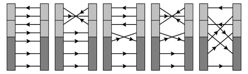
Figure 13: Schematic representation of the 7-quark contributions to the normalization.

Let us find the signs. These prototype diagrams have been chosen such that color contractions do not affect the sign. The first diagram is obviously positive (no crossing). The second one has three crossings (they are degenerate in the drawing but it does not change anything considering one or three crossings since the important thing is that it is odd) and is thus negative. So is the third one with its unique crossing. The fourth diagram has four crossings and is thus positive. The last one has six crossings and is thus also positive.

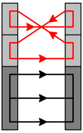
Figure 14: The color factor of this diagram is $3!\cdot 3$ since one has the valence circuit and an independent circuit.

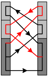
Figure 15: The color contractions in this diagram give a minus factor because of interchange of two valence quarks.

Following rule 2 there must be $5!2!=240$ contractions. Indeed, there are 12 of the first and second types while there are 72 of the other ones. Thus we have $2\cdot 12+3\cdot 72=240$ contractions as expected.

The color factor of the first diagram is $3!\cdot 3\cdot 3=54$ since there are two independent circuits. The color factor of the second one is only $3!\cdot 3=18$ since there is only one independent circuit as one can see on Fig. 15. The third diagram has also a unique independent circuit and thus a color factor of $3!\cdot 3=18$. For the two last diagrams there are no more independent circuit and have consequently a color factor of $3!=6$.

We close this appendix by considering the diagram in Fig. 15. Since two valence quarks are exchanged, it must belong to the fifth type of diagrams. There are seven crossings and thus a negative sign while the fifth type of diagrams is positive. In fact, for this particular diagram, the color contractions gives an additional minus sign since the third quark on the left is contracted with the second on the right $\epsilon^{\alpha_{1}\alpha_{2}\alpha_{3}}\epsilon_{\alpha_{1}\alpha_{3}\alpha_{2}}=-6$.

References

[1] D. Diakonov and V. Petrov, Phys. Lett. B147
(1984) 351; Nucl. Phys. B272 (1986) 457.
[2] E.H. Lieb, Rev. Mod. Phys. 53 (1981)
603;
[3] E. Witten, Nucl. Phys. B223 (1983) 433.
[4] D. Diakonov and V. Petrov, JETP Lett. 43 (1986) 57 [Pisma Zh. Eksp. Teor. Fiz. 43 (1986) 57]; D.
Diakonov, V. Petrov and P. Pobylitsa, Nucl. Phys. B306 (1988)
809;D. Diakonov and V. Petrov, in Handbook of QCD, ed. M. Shifman,
World Scientific, Singapore (2001), vol. 1, p. 359,
hep-ph/0009006.
[5] D. Diakonov, V. Petrov and M. Praszalowicz, Nucl. Phys. B323 (1989) 53.
[6] M. Wakamatsu and H. Yoshiki, Nucl. Phys. A524
(1991) 561. The first qualitative explanation of the spin crisis
from the Skyrme model point of view, namely zero fraction of proton
spin carried by quarks, was given in: S.J. Brodsky, J.R. Ellis and
M. Karliner, Phys. Lett. B206 (1988) 309. In the Chiral Quark
Soliton Model the fraction of spin carried by quarks is not
identically zero but small.
[7] D. Diakonov, Talk at the APS meeting, Denver, May 1-2
2004, hep-ph/0406043.
[8] C. Christov, A. Blotz, H.-C. Kim, P.
Pobylitsa, T. Watabe, Th. Meissner, E. Ruiz Arriola and K. Goeke,
Prog. Part. Nucl. Phys. 37 (1996) 91, hep-ph/9604441.
[9] D. Diakonov, V. Petrov, P. Pobylitsa, M. Polyakov
and C. Weiss, Nucl. Phys. B480 (1996) 341,
hep-ph/9606314; Phys. Rev. D56 (1997) 4069,
hep-ph/9703420.
[10] K. Goeke, M. Polyakov and M. Vanderhaegen, Prog.
Part. Nucl. Phys. 47 (2001) 401, hep-ph/0106012.
[11] D. Diakonov and V. Petrov, Phys. Rev. D72 (2005) 074009, hep-ph/0505201.
[12] E. Guadagnini, Nucl. Phys. B236 (1984)
35; L.C. Biedenharn, Y. Dothan and A. Stern, Phys. Lett. B146
(1984) 289; P.O. Mazur, M.A. Nowak and M. Praszalowicz, Phys. Lett.
B147 (1984) 137; A.V. Manohar, Nucl. Phys. B248 (1984)
19; M. Chemtob, Nucl. Phys. B256 (1985) 600; S. Jain and S.R.
Wadia, Nucl. Phys. B258 (1985) 713; D. Diakonov and V. Petrov,
Baryons as solitons, preprint LNPI-967 (1984), published in
Elementary Particles, Proc. 12th ITEP Winter School,
Energoatomizdat, Moscow (1985) pp.50-93.
[13] V. Petrov and M. Polyakov,
hep-ph/0307077.
[14] D. Diakonov and V. Petrov, Annalen des Phys. 13 (2004)
637, hep-ph/0409362.
[15] D. Diakonov, in: Continuous Advances in QCD
2004, ed. T. Gherghetta, World Scientific (2004) p. 369,
hep-ph/0408219.