Renormalization effects on neutrino masses and mixing in a string-inspired SU$(4)\times$SU$(2)_{L}\times$SU$(2)_{R}\times$U$(1)_{X}$ model

Abstract

We discuss renormalization effects on neutrino masses and mixing angles in a supersymmetric string-inspired SU$(4)\times$SU$(2)_{L}\times$SU$(2)_{R}\times$U$(1)_{X}$ model, with matter in fundamental and antisymmetric tensor representations and singlet Higgs fields charged under the anomalous $U(1)_{X}$ family symmetry. The quark, lepton and neutrino Yukawa matrices are distinguished by different Clebsch-Gordan coefficients. The presence of a second $U(1)_{X}$ breaking singlet with fractional charge allows a more realistic, hierarchical light neutrino mass spectrum with bi-large mixing. By numerical investigation we find a region in the model parameter space where the neutrino mass-squared differences and mixing angles at low energy are consistent with experimental data.

The experimentally measured values of gauge coupling constants $\alpha_{3},\alpha_{em}$, and the weak mixing angle $\sin^{2}\theta_{W}$ are correctly predicted in the Minimal Supersymmetric Standard Model (MSSM), assuming a unification scale of the order $10^{16}$ GeV. Moreover, the existing data from neutrino oscillation experiments provide an important clue to physics beyond the successful Standard Model (SM) and MSSM.

Experimental data on atmospheric and solar neutrino oscillations Bahcall:2004ut imply tiny but non-zero neutrino mass-squared differences $\Delta\,m^{2}_{\nu_{ij}}$. The negligible size of the neutrino masses, as compared to those of quarks and charged leptons, might suggest that a theory beyond MSSM should incorporate the right-handed neutrinos and an appropriate (see-saw) mechanism to suppress adequately the neutrino masses. Moreover, the observed large neutrino mixing angles $\theta_{\nu_{12}},\theta_{\nu_{23}}$ present challenges for additional symmetries and a unified framework in which neutrinos and quarks form part of same multiplet. Examples of higher symmetries including the SM gauge group and incorporating the right-handed neutrino in the fermion spectrum, are the partially unified Pati–Salam model, based on $SU(4)\times SU(2)_{L}\times SU(2)_{R}$ Pati:1974yy , and the fully unified $SO(10)$. When embedded into perturbative string or D-brane models, these may be extended by additional abelian or discrete fermion family symmetries. Thus fermion masses and mixing angles can be compared to the predictions of various types of models with full or partial gauge unification and flavor symmetries.

Recently some models have been proposed to explain the presence of large mixing angles in the neutrino sector, in contrast to the smaller quark mixings. For example, the mixing angle $\theta_{\nu_{12}}$ and the Cabibbo mixing $\theta_{C}$ could satisfy the so called Quark-Lepton Complementarity (QLC) relation $\theta_{\nu_{12}}+\theta_{C}\approx\frac{\pi}{4}$ Petcov:1993rk . It has been shown Minakata:2004xt that this relation can be reproduced if some symmetry exists among quarks and leptons. Attempts to realize QLC in the context of models unifying quarks and leptons such as Pati-Salam have been made Antusch:2005ca .

As another possibility, the symmetry $L_{e}-L_{\mu}-L_{\tau}$ implies an inverted neutrino mass hierarchy and bimaximal mixing $\theta_{\nu_{12}}=\theta_{\nu_{23}}=\frac{\pi}{4}$, with $\theta_{\nu_{13}}=0$ lelmlt . This symmetry alone does not give a consistent description of current experimental data, but additional corrections and renormalization effects have still to be taken into account. It has been shown Leontaris:2004rd in the context of MSSM extended by a spontaneously broken $U(1)_{X}$ factor, that the neutrino sector respects an $L_{e}-L_{\mu}-L_{\tau}$ symmetry. Small corrections from other singlet vevs, which are usually present in a string spectrum, can lead to a soft breaking of this symmetry and describe accurately the experimental neutrino data.

Another important issue is the renormalization group (RG) flow of the neutrino parameters from the high energy scale where the neutrino mass matrices are formed, down to their low energy measured values. One can attempt to determine the neutrino mass matrices from experimental data directly at the weak scale. However, the Yukawa couplings and other relevant parameters are not known at the unification scale. A knowledge of these quantities at the unification mass could provide a clue for the structure of the unified or partially unified theory and the exact (family) symmetries determining the neutrino mass matrices at the GUT scale. Attempts to determine the neutrino mass parameters in a top-bottom or bottom-up approach have recently discussed in the literature Antusch:2005gp ; Mei:2005qp ; Ellis:2005dr .

In this paper we investigate further the neutrino mass spectrum of a model with gauge symmetry $SU(4)\times SU(2)\times SU(2)\times U(1)_{X}$ based on the 4-4-2 models Antoniadis:1988cm ; Allanach:1995ch ; Allanach:1996hz , whose implications for quark and lepton masses were recently investigated in Dent:2004dn . These models present several attractive features. Firstly, only ”small” Higgs representations are needed and these commonly arise in string models. Secondly, third generation fermion Yukawa couplings are unified AllanachKQuad up to small corrections. Unification of gauge couplings is allowed and, if one assumes the model embedded in supersymmetric string, might be predicted LTracas . Furthermore, the doublet-triplet splitting problem is absent.

In string derived models a large number of neutral singlet fields carrying quantum numbers only under U$(1)_{X}$ appear in the spectrum of the effective field theory model. D- and F-flatness conditions require some of them to obtain non-zero vevs of the order of the U$(1)_{X}$ breaking scale. In the present model, in order to describe accurately the low energy neutrino data we introduce two such singlets charged under U$(1)_{X}$ Irges:1998ax . The previous model Dent:2004dn with one such singlet could easily give rise to a spectrum of light neutrinos with normal hierarchy and bi-large mixing. However, after study of the renormalization group (RG) evolution and unification it was found that the scale of light neutrino masses too large to be compatible with observation. If we impose the correct scale of light neutrino masses, then some heavy right-handed neutrinos (RHN) would have masses above the unification scale, which is incompatible with our effective field theory approach.

Thus three a priori independent expansion parameters arise from the superpotential, two coming from the singlets and one from the Higgses which receive v.e.v.’s at the SU$(4)\times$SU$(2)_{R}$ breaking scale. In general, a nonrenormalizable operator may contain several products of the SU$(4)\times$SU$(2)_{R}$ breaking Higgses, and thus different contractions of gauge group indices are possible leading to different contributions depending on the Clebsch factors. We use a minimal set of nontrivial Clebsch factors to construct the Dirac mass matrices. Right-handed (SU$(2)_{L}$ singlet) neutrinos acquire Majorana masses through nonrenormalizable couplings to the U$(1)_{X}$-charged singlets and to Higgses, while light neutrinos will obtain masses via the see-saw mechanism.

The renormalization group equations (RGEs) for the neutrino masses and mixing angles above, between and below the see-saw scales are solved numerically, for several sets of order 1 parameters which specify the heavy RHN matrix. In each case the results at low energy are consistent with current experimental data, and provide further predictions for the 1-3 neutrino mixing angle and for neutrinoless double beta decay.

I Description of the model

In this section we present salient features of the string inspired Pati-Salam model extended by a U$(1)_{X}$ family-symmetry, the total gauge group being SU$(4)\times$SU$(2)_{L}\times$SU$(2)_{R}\times$U$(1)_{X}$. The field content includes three copies of $(4,2,1)+(\bar{4},1,2)$ representations to accommodate the three fermion generations $F_{i}+\bar{F}_{i}$ ($i=1,2,3$),

$$F_{i}=\left(\begin{array}[]{cccc}u_{i}&u_{i}&u_{i}&\nu_{i}\\ d_{i}&d_{i}&d_{i}&e_{i}\end{array}\right)_{\alpha_{i}},\ \bar{F}_{i}=\left(\begin{array}[]{cccc}u_{i}^{c}&u_{i}^{c}&u_{i}^{c}&\nu_{i}^{c}\\ d_{i}^{c}&d_{i}^{c}&d_{i}&e_{i}^{c}\end{array}\right)_{\bar{\alpha}_{i}}$$

where the subscripts $\alpha_{i}$, $\bar{\alpha}_{i}$ indicate the U$(1)_{X}$ charge. In order to break the Pati-Salam symmetry down to SM gauge group, Higgs fields $H=(4,1,2)$ and $\bar{H}=(\bar{4},1,2)$ are introduced

$$H=\left(\begin{array}[]{cccc}u_{H}&u_{H}&u_{H}&\nu_{H}\\ d_{H}&d_{H}&d_{H}&e_{H}\end{array}\right)_{x},\;\bar{H}=\left(\begin{array}[]{cccc}u_{\bar{H}}^{c}&u_{\bar{H}}^{c}&u_{\bar{H}}^{c}&\nu_{\bar{H}}^{c}\par\\ d_{\bar{H}}^{c}&d_{\bar{H}}^{c}&d_{\bar{H}}&e_{\bar{H}}^{c}\end{array}\right)_{\bar{x}}$$ (5)

which acquire vevs of the order $M_{G}$ along their neutral components

$$\langle H\rangle=\langle\nu_{H}\rangle=M_{G},\ \langle\bar{H}\rangle=\langle\nu_{\bar{H}}\rangle=M_{G}.$$ (6)

The Higgs sector also includes the $h=(1,\bar{2},2)$ field which after the breaking of the PS symmetry is decomposed to the two Higgs superfields of the MSSM. Further, two $D=(6,1,1)$ scalar fields are introduced to give mass to color triplet components of $H$ and $\bar{H}$ via the terms $HHD$ and $\bar{H}\bar{H}D$ Antoniadis:1988cm .

Finally, we introduce two scalar singlet fields $\phi$, $\chi$, charged under U$(1)_{X}$ whose vevs will play a crucial role in the fermion mass matrices through non-renormalizable terms of the superpotential. In the stable SUSY vacuum the two singlets obtain vevs to satisfy the D-flatness condition including the anomalous Fayet-Iliopoulos term DineSW . The anomalous D-flatness conditions allow solutions where the vevs of the conjugate fields $\bar{\phi}$ and $\bar{\chi}$ are zero and we will restrict our analysis to this case. Note that in general a string model may have more than two singlets and more than one set of Higgses $H_{i}$, $\bar{H}_{i}$, with different U$(1)_{X}$ charge. All such fields may in principle also obtain vevs, however we find that two of them are sufficient to give a set of mass matrices in accordance with all experimental data. Hence we consider any additional singlet vevs to be significantly smaller.

The Higgses $H_{i}$, $\bar{H}_{i}$ may obtain masses through $H\bar{H}\phi$, $H\bar{H}\chi$ and $H\bar{H}\phi\chi$ couplings. However, in order to break the Pati-Salam group while preserving SUSY we require that one $H$-$\bar{H}$ pair be massless at this level. This “symmetry-breaking” Higgs pair could be a linear combination of fields with different U$(1)_{X}$ charges, which would in general complicate the expressions for fermion masses. The chiral spectrum is summarized in Table 1. We choose the charge of the Higgs field $h$ to be $-\alpha_{3}-\bar{\alpha}_{3}$ so that that the 3rd. generation coupling $F_{3}\bar{F}_{3}h$ is allowed at tree-level.

Table 1: Field content and U$(1)_{X}$ charges

	SU$(4)$	SU$(2)_{L}$	SU$(2)_{R}$	U$(1)_{X}$
$F_{i}$	4	2	1	$\alpha_{i}$
$\bar{F}_{i}$	$\bar{4}$	1	$\bar{2}$	$\bar{\alpha}_{i}$
$H$	4	1	2	$x$
$\bar{H}$	$\bar{4}$	1	$\bar{2}$	$\bar{x}$
$\phi$	1	1	1	$z$
$\chi$	1	1	1	$z^{\prime}$
$h$	1	$\bar{2}$	2	$-\alpha_{3}-\bar{\alpha}_{3}$
$D_{1}$	6	1	1	$-2x$
$D_{2}$	6	1	1	$-2\bar{x}$

We now turn to the terms in the superpotential which can give rise to fermion masses. Dirac type mass terms arise after electroweak symmetry-breaking from couplings of the form

$${\cal W}_{D}=y_{0}^{33}F_{3}\bar{F}_{3}h+F_{i}\bar{F}_{j}h\left(\sum_{m>0}y_{m}^{ij}\left(\frac{\phi}{M_{U}}\right)^{m}+\right.\\ \left.\sum_{m^{\prime}>0}y_{m^{\prime}}^{ij}\left(\frac{\chi}{M_{U}}\right)^{m^{\prime}}+\sum_{n>0}{y^{\prime}}_{n}^{ij}\left(\frac{H\bar{H}}{M_{U}^{2}}\right)^{n}+\right.\\ \left.\sum_{k,\ell>0}y_{k,\ell}^{ij}\left(\frac{\phi}{M_{U}}\right)^{k}\left(\frac{\chi}{M_{U}}\right)^{\ell}+\sum_{p,q>0}y_{p,q}^{ij}\left(\frac{H\bar{H}}{M_{U}^{2}}\right)^{p}\left(\frac{\phi}{M_{U}}\right)^{q}\right.\\ \left.+\sum_{r,s>0}y_{r,s}^{ij}\left(\frac{H\bar{H}}{M_{U}^{2}}\right)^{r}\left(\frac{\chi}{M_{U}}\right)^{s}+\cdots\right)$$ (7)

Apart from the heaviest generation, all masses arise at non-renormalizable level, suppressed by powers of the fundamental scale or unification scale $M_{U}$. The couplings $y_{m,m^{\prime}}^{ij}$, ${y^{\prime}}_{n}^{ij}$ etc. are non-vanishing and generically of order $1$ whenever the U$(1)_{X}$ charge of the corresponding operator vanishes, thus:

$$\alpha_{i}-\alpha_{3}+\bar{\alpha}_{j}-\bar{\alpha}_{3}=\{-mz,-m^{\prime}z^{\prime},-n(x+\bar{x}),\\ -kz-\ell z^{\prime},-p(x+\bar{x})-qz,-r(x+\bar{x})-sz^{\prime}\}.$$ (8)

Other higher-dimension operators may arise by multiplying any term by factors such as $(H\bar{H})^{\ell}\phi^{s}/M_{U}^{2\ell+s}$ where $\ell(x+\bar{x})+s\,z=0$. Such terms are negligible unless the leading term vanishes.

Neutrinos may in addition receive also Majorana type masses. These arise from the operators

$$W_{M}=\frac{\bar{F}_{i}\bar{F}_{j}HH}{M_{U}}\left(\mu_{0}^{ij}+\sum_{t>0}\mu_{t}^{ij}\left(\frac{\phi}{M_{U}}\right)^{t}\right.\\ \left.+\sum_{t^{\prime}>0}\mu_{t^{\prime}}^{ij}\left(\frac{\chi}{M_{U}}\right)^{t^{\prime}}+\sum_{w>0}{\mu^{\prime}}_{w}^{ij}\left(\frac{H\bar{H}}{M_{U}^{2}}\right)^{w}\right.\\ \left.+\sum_{k^{\prime},\ell^{\prime}>0}\mu_{k^{\prime},\ell^{\prime}}^{ij}\left(\frac{\phi}{M_{U}}\right)^{k^{\prime}}\left(\frac{\chi}{M_{U}}\right)^{\ell^{\prime}}\right.\\ \left.+\sum_{p^{\prime},q^{\prime}>0}\mu_{p^{\prime},q^{\prime}}^{ij}\left(\frac{H\bar{H}}{M_{U}^{2}}\right)^{p^{\prime}}\left(\frac{\phi}{M_{U}}\right)^{q^{\prime}}\right.\\ \left.+\sum_{r,s>0}\mu_{r^{\prime},s^{\prime}}^{ij}\left(\frac{H\bar{H}}{M_{U}^{2}}\right)^{r^{\prime}}\left(\frac{\chi}{M_{U}}\right)^{s^{\prime}}+\cdots\right).$$ (9)

Couplings of this type are non-vanishing whenever the following conditions are satisfied:

$$\bar{\alpha}_{i}+\bar{\alpha}_{j}+2x=\{-tz,-t^{\prime}z^{\prime},-w(x+\bar{x}),\\ -k^{\prime}z-\ell^{\prime}z^{\prime}-p^{\prime}(x+\bar{x})-q^{\prime}z,-r^{\prime}(x+\bar{x})-s^{\prime}z^{\prime}\}.$$ (10)

II Fermion mass matrices

II.1 General structure

As can be seen from the superpotential Yukawa couplings (7) and (9), three different expansion parameters appear in the construction of the fermion mass matrices. These are

$$\epsilon\equiv\frac{\langle\phi\rangle}{M_{U}},\ \ \ \epsilon^{\prime}\equiv\frac{M_{\rm G}^{2}}{M_{U}^{2}},\ \ \ \epsilon^{\prime\prime}\equiv\frac{\langle\chi\rangle}{M_{U}}$$ (11)

given $\langle H\bar{H}\rangle=M_{G}^{2}$. Note that, for non-renormalizable Dirac mass terms involving several products of $H\bar{H}/M_{U}^{2}$, the gauge group indices may be contracted in different ways Allanach:1996hz . This can lead to different contributions to the up, down quarks and charged leptons, depending on the Clebsch factors $C^{ij}_{n(u,d,e,\nu)}$ multiplying the effective Yukawa couplings. Also, although the Clebsch coefficient for a particular operator $O_{n}$ may vanish at order $n$, the coefficient for the operator $O_{(n+p);q}$ containing $p$ additional factors $(H\bar{H})$ and $q$ factors of $\phi$ and/or $\chi$ is generically nonzero.

In our analysis we wish to estimate the effects of the second singlet ($\chi$) contributions on the neutrino sector as compared to the analysis presented in Dent:2004dn without affecting essentially the results in the quark sector. In order to obtain a set of fermion mass matrices with the minimum number of new operators, we assume fractional $U(1)_{X}$ charges for $H,\bar{H}$ and $\chi$ fields, while the combination $H\bar{H}$ and the singlet $\phi$ are assumed to have integer charges. Thus $\alpha_{i}$, $\bar{\alpha}_{i}$, $x+\bar{x}$ and $z$ are integers, while $z^{\prime}$, $x$ and $\bar{x}$ are fractional. As a result, the Dirac mass terms involving vevs of $\chi$ are expected to be subleading compared to other terms. Suppressing higher-order terms involving products of $\epsilon,\epsilon^{\prime}$ and $\epsilon^{\prime\prime}$, the Dirac mass terms at the unification scale are

$$m_{ij} \approx \delta_{i3}\delta_{j3}m_{3}+\left(\epsilon^{m}+(\epsilon^{\prime\prime})^{m^{\prime}}+C_{ij}(\epsilon^{\prime})^{n}\right)\,v_{u,d}$$ (12)

where $m_{3}\equiv v_{u,d}y_{0}^{33}$, with $v_{u}$ and $v_{d}$ being the up-type and down-type Higgs vevs respectively, and we omit the order-one Yukawa coefficients $y^{ij}_{m}$ etc. for simplicity.

The Majorana mass terms are proportional to the combination $HH$ (see Eq. (9)) which has fractional $U(1)_{X}$ charge. Thus, terms proportional to $\chi/M_{U}$ become now important for the structure of the mass matrix. The general form of the Majorana mass matrix is then

$$M_{N}\approx M_{R}\left(\mu_{t}^{ij}\epsilon^{t}+\mu_{t^{\prime}}^{ij}(\epsilon^{\prime\prime})^{t^{\prime}}+{\mu^{\prime}}_{w}^{ij}(\epsilon^{\prime})^{w}\right.\\ \left.+\mu_{k^{\prime},l^{\prime}}^{ij}\epsilon^{k^{\prime}}(\epsilon^{\prime\prime})^{l^{\prime}}+\mu_{p^{\prime},q^{\prime}}^{ij}(\epsilon^{\prime})^{p^{\prime}}\epsilon^{q^{\prime}}+\mu_{r^{\prime},s^{\prime}}^{ij}(\epsilon^{\prime})^{r^{\prime}}(\epsilon^{\prime\prime})^{s^{\prime}}\right)$$ (13)

where we define $M_{R}\equiv M_{\rm G}^{2}/M_{U}\equiv\epsilon^{\prime}M_{U}$.

II.2 Specific choice of $U(1)_{X}$ charges

Before we proceed to a specific, viable set of mass matrices, we first make use of the observation Dent:2004dn that the form of the fermion mass terms above is invariant under the shifts

$$\alpha_{i}\rightarrow\alpha_{i}+\zeta,\ \bar{\alpha}_{i}\rightarrow\bar{\alpha}_{i}+\bar{\zeta},\ x\rightarrow x-\bar{\zeta},\ \bar{x}\rightarrow\bar{x}+\bar{\zeta}$$ (14)

so that we are free to assign $\alpha_{3}=\bar{\alpha}_{3}=0$. We further fix $x+\bar{x}=1$ and $z=-1$; we will choose the values of $x$ and $z^{\prime}$ to be fractional such that the v.e.v. of $\chi$ only affects the overall scale of neutrino masses, as explained below.

The charge entries of the common Dirac mass matrix for quarks, charged leptons and neutrinos are then

$$Q_{X}[M_{D}]=\begin{pmatrix}-6&-3&-4\\ -5&-2&-3\\ -2&1&0\end{pmatrix},$$ (15)

and the charge matrix for heavy neutrino Majorana masses is

$$Q_{X}[M_{N}]=2x+\begin{pmatrix}-4&-1&-2\\ -1&2&1\\ -2&1&0\end{pmatrix}.$$ (16)

Now, we relate $\epsilon,\epsilon^{\prime},\epsilon^{\prime\prime}$ with a single expansion parameter $\eta$, assuming the relations

$$\epsilon=b_{1}\sqrt{\eta},\ \epsilon^{\prime\prime}\equiv b_{2}\eta,\ \epsilon^{\prime}=\sqrt{\eta}$$ (17)

where $b_{1}$, $b_{2}$ are numerical coefficients of order one. Then the effective Yukawa couplings for quarks and leptons may include terms

$$Y_{f}^{ij}=b_{1}^{m}\eta^{m/2}+b_{1}^{m+1}\eta^{1+m/2}+C_{f}^{ij}\eta^{n/2}+b_{1}\eta^{1+n/2}+\cdots$$ (18)

with $f=u,d,e,\nu$, up to order 1 coefficients $y_{f}^{ij}$. Which of these terms survives, depends on the sign of the charge of the corresponding operator. For a negative charge entry, the first two terms are not allowed and only the third and fourth contribute. Further, if a particular $C_{f}^{ij}$ coefficient is zero, then we consider only the fourth term.

Therefore, we need to specify the Clebsch-Gordan coefficients $C^{ij}_{f}$ for the terms involving powers of $\langle{H\bar{H}}\rangle/M_{U}^{2}$. These coefficients could be found if the fundamental theory was completely specified at the unification or string scale. In the absence of a specific string model, here we present a minimal number of operators which lead to a simple and viable set of mass matrices. Up to possible complex phases, we choose $C_{d}^{12}=C_{d}^{22}=\frac{1}{3}$, $C_{u}^{23}=3$ and $C_{u}^{11}=C_{u}^{12}=C_{u}^{21}=C_{u}^{22}=C_{u}^{31}=C_{\nu}^{22}=C_{\nu}^{31}=0$ with all others being equal to unity. The effective Yukawa matrices at the GUT scale obtained under the above assumptions are

$$Y_{u}=\begin{pmatrix}b_{1}\eta^{4}&b_{1}\eta^{5/2}&\eta^{2}\\ b_{1}\eta^{7/2}&b_{1}\eta^{2}&3\eta^{3/2}\\ b_{1}\eta^{2}&b_{1}\eta^{1/2}&1\end{pmatrix},\ Y_{d}=\begin{pmatrix}\eta^{3}&\frac{\eta^{3/2}}{3}&\eta^{2}\\ \eta^{5/2}&\frac{\eta}{3}&\eta^{3/2}\\ \eta&b_{1}\eta^{1/2}&1\end{pmatrix},$$

$$Y_{e}=\begin{pmatrix}\eta^{3}&\eta^{3/2}&\eta^{2}\\ \eta^{5/2}&\eta&\eta^{3/2}\\ \eta&b_{1}\eta^{1/2}&1\end{pmatrix},\ Y_{\nu}=\begin{pmatrix}\eta^{3}&\eta^{3/2}&\eta^{2}\\ \eta^{5/2}&b_{1}\eta^{2}&\eta^{3/2}\\ b_{1}\eta^{2}&b_{1}\eta^{1/2}&1\end{pmatrix}$$ (19)

where we suppress order one coefficients. The quark sector as well as the neutrino sector were studied in Dent:2004dn . However, full renormalization group effects were not calculated for the neutrino sector and as it turns out one singlet is inadequate to accommodate the low energy data. Consequently, we introduced the second singlet $\chi$, with fractional charge, whose v.e.v. affects only the overall scale of neutrino masses.

The desired matrix for the right handed Majorana neutrinos may result from more than one choice of charge for the $H$ field and the $\chi$ singlet field. These can be seen in Table 2.

$Q_{X}[H]$	$-\frac{2}{3}$	$-\frac{4}{3}$	$-\frac{5}{3}$	$-\frac{6}{5}$	$-\frac{7}{8}$	$-\frac{1}{4}$	$-\frac{3}{4}$
$Q_{X}[\chi]$	$-\frac{5}{3}$	$-\frac{1}{3}$	$\frac{1}{3}$	$-\frac{3}{5}$	$-\frac{5}{4}$	$-\frac{5}{2}$	$-\frac{3}{2}$

Table 2: Possible choices for the U(1)_X charges of the $H$ and $\chi$ fields.

We choose the $H$ charge to be $x=-\frac{6}{5}$ so that $2\,x$ is non-integer, and set the $\chi$ singlet charge to $-\frac{3}{5}$. The analysis for the quarks and charged leptons remains the as in Dent:2004dn since operators with nonzero powers $\chi^{r}$ do not exist for powers $r<5$ and are negligible compared to the leading terms.

With these assignments, the charge entries of the heavy Majorana matrix Eq. (16) are:

$$Q_{X}[M_{N}]=\left(\begin{array}[]{ccc}-\frac{32}{5}&-\frac{17}{5}&-\frac{22}{5}\\ -\frac{17}{5}&-\frac{2}{5}&-\frac{7}{5}\\ -\frac{22}{5}&-\frac{7}{5}&-\frac{12}{5}\end{array}\right).$$ (20)

Due to the fractional $U(1)_{X}$ charges contributions from $\phi$ or $H\bar{H}$ alone vanish. However, we also have the singlets $H\bar{H}\chi/M_{U}^{3}$ with vev $b_{2}\,\eta^{3/2}$ and $\phi\chi/M_{U}^{2}$ with a vev $b_{1}b_{2}\,\eta^{2}$, while for some entries one may have to consider higher order terms since the leading order will be vanishing. In Table 3 we explicitly write the operator for every entry of $M_{N}$. The Majorana right-handed neutrino mass matrix is then

$$M_{N}=\left(\begin{array}[]{ccc}\mu_{11}\eta^{9/2}&\mu_{12}\eta^{3}&\mu_{13}\eta^{7/2}\\ \mu_{12}\eta^{3}&\mu_{22}\eta^{3/2}&\mu_{23}\eta^{2}\\ \mu_{13}\eta^{7/2}&\mu_{23}\eta^{2}&\eta^{5/2}\end{array}\right)b_{2}M_{R}$$ (21)

with $M_{R}=\epsilon^{\prime}M_{U}=\sqrt{\eta}M_{U}$.

Having defined the Dirac and heavy Majorana mass matrices for the neutrinos, it is straightforward to obtain the light Majorana mass matrix from the see-saw formula

$$m_{\nu}=-m_{D\nu}M_{N}^{-1}m_{D\nu}^{T}$$ (22)

at the GUT scale.

$M_{N}$ entry	Operator	vev
$M_{N}^{11}$	$\left(\frac{H\bar{H}}{M_{U}^{2}}\right)^{6}\frac{\chi}{M_{U}}$	$b_{2}\eta^{9/2}$
$M_{N}^{12}$	$\left(\frac{H\bar{H}}{M_{U}^{2}}\right)^{4}\frac{\chi}{M_{U}}$	$b_{2}\eta^{3}$
$M_{N}^{13}$	$\left(\frac{H\bar{H}}{M_{U}^{2}}\right)^{5}\frac{\chi}{M_{U}}$	$b_{2}\eta^{7/2}$
$M_{N}^{22}$	$\left(\frac{H\bar{H}}{M_{U}^{2}}\right)\frac{\chi}{M_{U}}$	$b_{2}\eta^{3/2}$
$M_{N}^{23}$	$\left(\frac{H\bar{H}}{M_{U}^{2}}\right)^{2}\frac{\chi}{M_{U}}$	$b_{2}\eta^{2}$
$M_{N}^{33}$	$\left(\frac{H\bar{H}}{M_{U}^{2}}\right)^{3}\frac{\chi}{M_{U}}$	$b_{2}\eta^{5/2}$

Table 3: Operators producing the Majorana right handed neutrino matrix $M_{N}$.

II.3 Setting the expansion parameters

Given the fermion mass textures in terms of the $U(1)_{X}$ charges and expansion parameters, we need now to determine the values of the latter in order to obtain consistency with the low energy experimentally known quantities (masses and mixing angles). Note that the coefficient $b_{2}$ defined in Eq. (17) will determine the overall neutrino mass scale through Eq. (21).

Consistency with the measured values of quark masses and mixings fixes the value of $\eta\approx 5\times 10^{-2}$: for example the CKM mixing angle $\theta_{12}$ is given by $\sqrt{\eta}\approx 0.22$ up to small corrections Dent:2004dn . Hence the ratio of the SU$(4)$ breaking scale $M_{G}$ to the fundamental scale $M_{U}$ is also fixed through $\frac{M_{G}^{2}}{M_{U}^{2}}=\sqrt{\eta}\approx 0.22$: the Pati-Salam group is unbroken over only a small range of energy. We perform a renormalization group analysis in order to check the consistency of this prediction with the low-energy values of the gauge couplings $\alpha_{s}$, $\alpha_{em}$ and the weak mixing angle $\sin^{2}\theta_{W}$ Eidelman

$$\sin^{2}\theta_{W}=0.23120,\ \alpha_{3}=0.118\pm 0.003,\ a_{em}=\frac{1}{127.906}.$$

If the underlying model at $M_{U}$ has a single unified gauge coupling, then $M_{G}$ is fixed to be just below the unification scale according to the analysis of gauge coupling unification in the MSSM. Because of this fact, the low energy measured range for $\alpha_{3}$ affects the unification of the gauge couplings. Thus, we add the following extra states

$$h_{L}=(1,2,1),\ \ h_{R}=(1,1,2)$$

which are usually present in a string spectrum Antoniadis:1988cm . It turns out that we need 4 of each of these extra states for $M_{G}=9.32\times 10^{15}$ GeV to be consistent with the value of $\epsilon^{\prime}$ deduced from quark mass matrices.

In Figure 1 we plot the evolution of the gauge couplings from $M_{Z}$ to $M_{U}$. In Figure 2 we show in more detail the evolution of the gauge couplings in the Pati-Salam energy region. The two bands for the $\alpha_{4}$ and $\alpha_{2R}$ couplings are due to strong coupling uncertainty at $M_{Z}$. For $\alpha_{3}(M_{Z})=0.1176$, as can be seen from Figure 3, we obtain $M_{U}=1.96\times 10^{16}$ GeV.

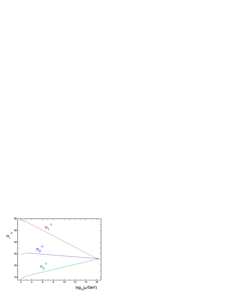
Figure 1: Evolution of the gauge couplings. The two lines for $\alpha_{3}$ indicate the range of initial conditions at $M_{Z}$.

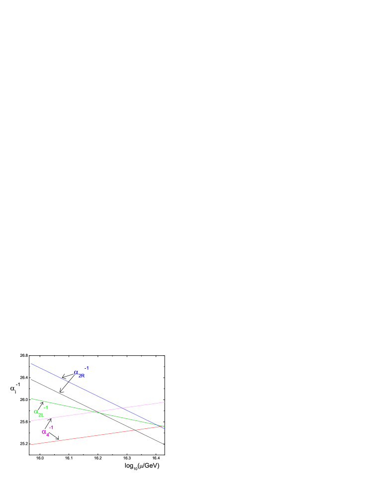
Figure 2: Close-up of the gauge couplings in the Pati-Salam energy region.

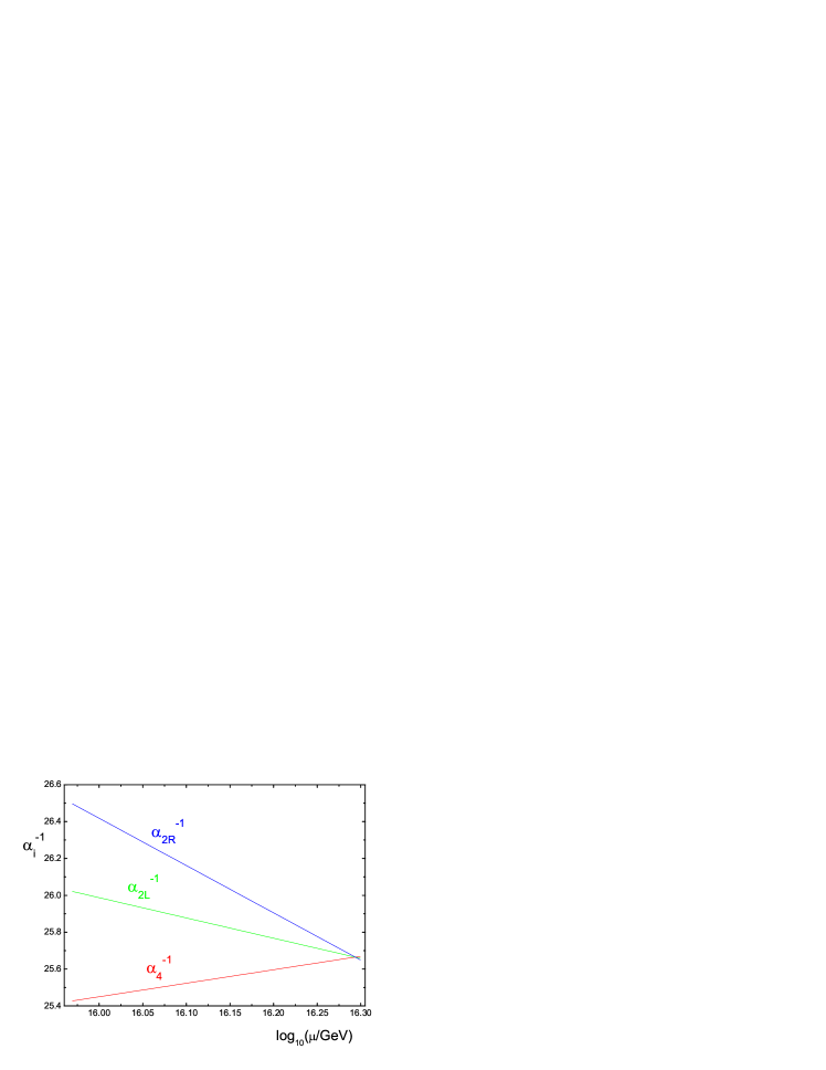
Figure 3: The unification point of Pati-Salam gauge couplings for $\alpha_{3}(M_{Z})=0.1176$.

The remaining parameters to be determined are $b_{1}$, $b_{2}$ and $\mu_{ij}$ of the right handed neutrino mass matrix. We find that $M_{N}$ is proportional to $b_{2}$, $M_{N}\approx b_{2}M_{R}M_{N}^{\prime}$, thus $b_{2}$ is related to the scale of the light matrix $m_{\nu}$. Also, the choice $b_{1}\approx 1.1$ leads to agreement with the data, while implying $\epsilon=1.1\sqrt{\eta}\approx 0.25$.

III Running of neutrino masses and mixing angles

One of the problems one encounters when searching for a specific mass matrix for the light neutrinos via the see-saw formula is the effects induced by the renormalization group equations. The low energy neutrino data could be considerably different from the results at the see-saw scale. The running of neutrino masses and mixing angles has been extensively discussed for energies below the seesaw scales below ; Antusch:2002rr ; Antusch:2003kp as well as above above ; Antusch:2005gp ; Mei:2005qp . The running of the effective neutrino mass matrix $m_{\nu}$ above and between the see-saw scales is split into two terms,

$$m_{\nu}\,=\,-\frac{v^{2}}{4}\left(\,\accentset{(n)}{\kappa}+2\,\accentset{(n)}{Y}_{\nu}\accentset{(n)}{M}^{-1}\accentset{(n)}{Y}_{\nu}^{T}\right)\;.$$ (23)

where $\kappa$ is related to the coefficient of the effective 5 dimensional operator $LLh_{u}h_{u}$, $(n)$ labels the effective field theories with $M_{n}$ right handed neutrino integrated out ($M_{n}\geq M_{n-1}\geq M_{n-2},\ldots$) and $\accentset{(n)}{Y}_{\nu}$ are the neutrino couplings at an energy scale $M$ between two RH neutrino masses $M_{n}\geq M\geq M_{n-1}$, while $\accentset{(n)}{Y}_{\nu}=0$ below the lightest RH neutrino mass. These effective parameters govern the evolution below the highest seesaw scale and obey the differential equation below ; Antusch:2002rr ; Antusch:2003kp

$$16\pi^{2}\frac{d\accentset{(n)}{X}}{dt}=(Y_{e}Y_{e}^{\dagger}+\accentset{(n)}{Y}_{\nu}\accentset{(n)}{Y}_{\nu}^{\dagger})^{T}\accentset{(n)}{X}+\accentset{(n)}{X}(Y_{e}Y_{e}^{\dagger}+\accentset{(n)}{Y}_{\nu}\accentset{(n)}{Y}_{\nu}^{\dagger})^{T}\\ +(2\mbox{\rm Tr}(\accentset{(n)}{Y}_{\nu}\accentset{(n)}{Y}_{\nu}^{\dagger}+3Y_{u}Y_{u}^{\dagger})-6/5g_{1}^{2}-6g_{2}^{2})\accentset{(n)}{X}$$ (24)

where $X=\kappa$, $Y_{\nu}M^{-1}Y_{\nu}^{T}$. The RGEs have been solved both numerically and also analytically Antusch:2003kp ; Antusch:2005gp ; Mei:2005qp . Numerically, below the lightest heavy RH neutrino mass large renormalization effects can be experienced only in the case of degenerate light neutrino masses for very large $\tan\beta$ Ellis:1999my ; Antusch:2003kp . Above this mass things are more complicated due to the non-trivial dependence of the heavy neutrino mass couplings, unless $M_{\nu^{c}}$ is diagonal. For the leptonic mixing angles, in the case of normal hierarchy relevant to our model, one expects negligible effects for the solar mixing angle while $\theta_{13}$ and $\theta_{23}$ are expected to run faster Ellis:2005dr .

On the other hand, studying the analytical expressions obtained after approximation, exactly the opposite behavior is predicted and the solar mixing angle receives larger renormalization effects than $\theta_{13}$ or $\theta_{23}$. However, possible cancellations may occur and enhancement or suppresion factors may appear, thus the numerical solutions may differ considerably from these estimates.

In our string-inspired model the Dirac and heavy Majorana mass matrices at the unification scale are parametrized in terms of order-1 superpotential coefficients $\mu_{ij}(M_{U})$ whose exact numerical values are not known. The flavour structure at the unification scale might also be different from that at the electroweak scale $M_{Z}$. Thus, even if the Yukawa parameters are determined at $M_{Z}$, to understand the structure of the theory at $M_{U}$, and consequently any possible family symmetry, we would certainly need the parameter values at $M_{U}$.

In this section we study the renormalization group flow of the neutrino mass matrices “top-down” from the Pati-Salam scale $M_{G}$ to the weak scale. We choose sets of values of the undetermined order 1 coefficients at the high scale and run the renormalization group equations down to $M_{Z}$ where we calculate $\Delta m_{\nu_{ij}}^{2}$ and $\theta_{\nu_{ij}}$ and compare them with the experimental values. Study of a bottom-up approach has been performed Ellis:2005dr and we will compare our results to this work. The renormalization group analyses of the neutrino parameters, successively integrating out the right handed neutrinos, is performed using the software packages REAP/MPT Antusch:2005gp .

$\bullet$ We generate appropriate numerical values for the coefficients $\mu_{11}$, $\mu_{12}$, $\mu_{13}$, $\mu_{22}$, $\mu_{23}$, so that after the evolution of $m_{\nu}$ to low energy we obtain values in agreement with the experimental data. The coefficient $\mu_{3}3$ is set to unity (which can always be done by adjusting the value of $b_{2}$). Experimentally acceptable solutions can be seen in Table 4. In Table 5 we present the resulting values of $\theta_{ij}$ and $\Delta m_{ij}^{2}$ at the scale $M_{Z}$. The mass-squared differences lie in the ranges $\Delta m_{atm}^{2}=[1.33-3.39]\times 10^{-3}$eV², $\Delta m_{sol}^{2}=[7.24-8.85]\times 10^{-5}$eV². These are consistent with the experimental data ${\Delta m_{atm,exp}^{2}}=[1.3-3.4]\times 10^{-3}$eV² and ${\Delta m_{sol,exp}^{2}}=[7.1-8.9]\times 10^{-5}$eV². The mixing angles are also found in the allowed ranges $\theta_{12}=[29.4-37.6]$, $\theta_{23}=[36.9-51.0]$ and $\theta_{13}=[0.86-12.50]$.

Solution	$\mu_{11}$	$\mu_{12}$	$\mu_{13}$	$\mu_{22}$	$\mu_{23}$
1.	0.10535	0.10972	0.86012	0.10491	0.91014
2.	0.11939	0.10954	0.80912	0.10683	0.93832
3.	0.10392	0.11787	0.97796	0.10512	0.98749
4.	0.09143	0.10962	0.87616	0.10063	0.93798
5.	0.12697	0.12745	0.99860	0.11652	0.99980
6.	0.10920	0.09638	1.00975	0.10238	0.93561
7.	0.10124	0.11682	0.98568	0.10688	0.99156
8.	0.12358	0.09514	0.99580	0.10434	0.95646
9.	0.13006	0.11973	1.02235	0.10378	0.89460
10.	0.12665	0.12137	1.00029	0.10695	0.91578

Table 4: Numerical values of parameters $\mu_{11}$, $\mu_{12}$, $\mu_{13}$, $\mu_{22}$, $\mu_{23}$ at $M_{G}$.

Soln.	$\Delta m_{atm}^{2}\cdot 10^{3}$	$\Delta m_{sol}^{2}\cdot 10^{5}$	$\theta_{12}$	$\theta_{13}$	$\theta_{23}$
1.	2.7149	7.9621	29.442	3.9859	44.114
2.	2.3145	7.9514	34.289	12.507	51.047
3.	1.8978	8.6141	30.560	0.8656	46.230
4.	3.0062	8.3217	34.347	1.8512	44.333
5.	3.3905	7.2468	30.245	2.9355	36.900
6.	3.2459	7.5351	34.296	1.3701	46.947
7.	2.0171	7.9464	34.432	1.0086	50.279
8.	1.3321	7.9060	37.646	6.1490	43.067
9.	2.4867	8.8561	29.592	5.6007	42.970
10.	2.1652	7.8869	29.189	3.1512	37.220

Table 5: Values of the physical parameters $\Delta m^{2}_{atm}$, $\Delta m^{2}_{sol}$, $\theta_{12}$, $\theta_{13}$, $\theta_{23}$ at $M_{Z}$ (mass units eV²).

$\bullet$ In figure (4) we plot the running of the three light neutrino Majorana masses ($m_{1}<m_{2}<m_{3}$) in the energy range $M_{G}-M_{Z}$. The initial (GUT) neutrino eigenmasses are all larger than their low energy values. Significant running is observed mainly for the heaviest eigenmass $m_{\nu_{3}}$. For experimentally acceptable mass-squared differences $\Delta m_{\nu_{ij}}^{2}$ at $M_{Z}$, in all cases their corresponding values at the GUT scale lie out of the acceptable range. In this scenario with hierarchical light neutrino masses, we find that large renormalization effects occur above the heavy neutrino threshold since the Yukawa couplings $Y_{\nu}$ are large and the second term in (23) dominates. Also, since $m_{\nu_{1}}<\sqrt{\Delta m^{2}_{sol}}$, the solar angle turns out to be more stable compared to the running of the $\theta_{23}$, as can be seen in Figure (5). These results are in agreement with the findings of Ellis:2005dr .

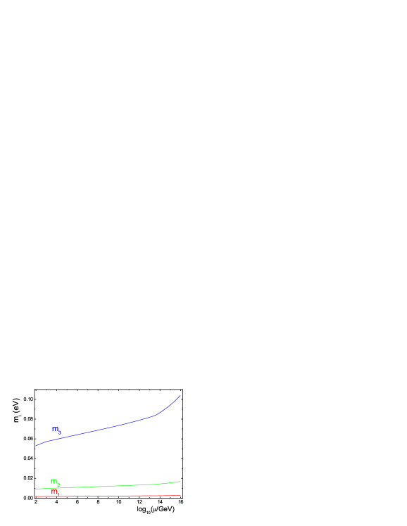
Figure 4: The running of the light neutrino masses.

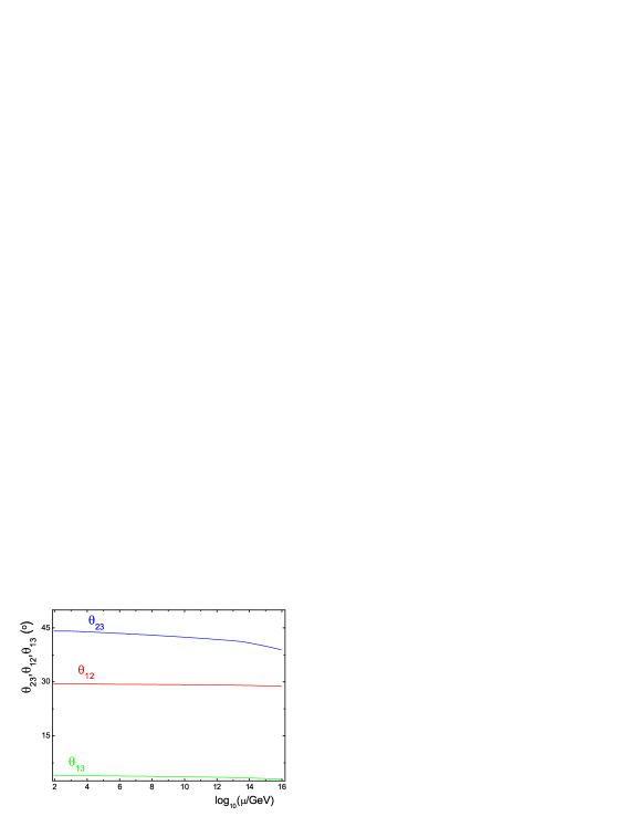
Figure 5: The evolution of the mixing angles.

Soln.	$\Delta m_{atm}^{2}(M_{G})\cdot 10^{3}$	$\Delta m_{sol}^{2}(M_{G})\cdot 10^{5}$	$\langle m\rangle$	$b_{2}$
1.	10.5294	27.6096	0.00361	3.41
2.	8.1987	30.1333	0.00633	2.88
3.	7.2533	31.6108	0.00607	1.50
4.	11.7749	30.4352	0.00753	1.28
5.	14.093	23.7416	0.00346	2.85
6.	12.347	28.2642	0.00822	1.26
7.	7.4256	30.855	0.00821	1.23
8.	5.2910	29.8775	0.00852	1.17
9.	9.74656	30.5418	0.00379	3.64
10.	8.99695	25.8838	0.00327	3.42

Table 6: Values of the physical parameters $\Delta m^{2}_{atm}$ and $\Delta m^{2}_{sol}$ at $M_{G}$; the effective neutrino mass $\langle m\rangle$ related to $\beta\beta_{0\nu}$ decay; and the parameter $b_{2}$ which determines the scale of the light matrix $m_{\nu}$.

$\bullet$ In figure (7) we plot the distribution $\Delta m_{atm}^{2}$ versus $\Delta m_{sol}^{2}$ at the two scales $M_{G}$ (Table 6) and $M_{Z}$ for the ten models of Table 4. We find that the hierarchy of the neutrino masses at the Pati-Salam breaking scale tends to be greater than that at low energies. Several models predict $\Delta m_{23}^{2}/\Delta m_{21}^{2}$ out of the experimental range at $M_{G}$, although after the running at $M_{Z}$ they are consistent with the data.

$\bullet$ Finally, we check the predictions of our model for the effective neutrino mass parameter relevant for $\beta\beta_{0\nu}$ decay. This parameter can be written in terms of the observable quantities as

$$|\langle m\rangle|=\left|(m_{1}\cos^{2}\theta_{\odot}+e^{i\alpha}\sqrt{\Delta m_{sol}}\sin^{2}\theta_{\odot})\cos^{2}\theta_{13}\right.\\ +\left.\sqrt{\Delta m_{atm}}\sin^{2}\theta_{13}e^{i\beta}\right|.$$ (25)

In the last column of Table (6) the $\beta\beta_{0\nu}$-decay predictions are presented for solutions 1-10. Many current experiments attempt to measure this quantity Petcov:2005yq ; the best current limit on the effective mass is given by the Heidelberg–Moscow collaboration heidmo

$$\langle m\rangle\leq 0.35\,z~{}\mbox{eV},$$ (26)

where the parameter $z={\cal O}(1)$ allows for uncertainty arising from nuclear matrix elements.

In a recent analysis of neutrinoless double beta decay Choubey:2005rq the allowable range of the effective mass parameter was given for specific scenarios. In the case of the normal hierarchy the bounds are

$$0<\langle m\rangle<0.007\,\mbox{eV}$$ (27)

thus our results are in the experimentally acceptable region.

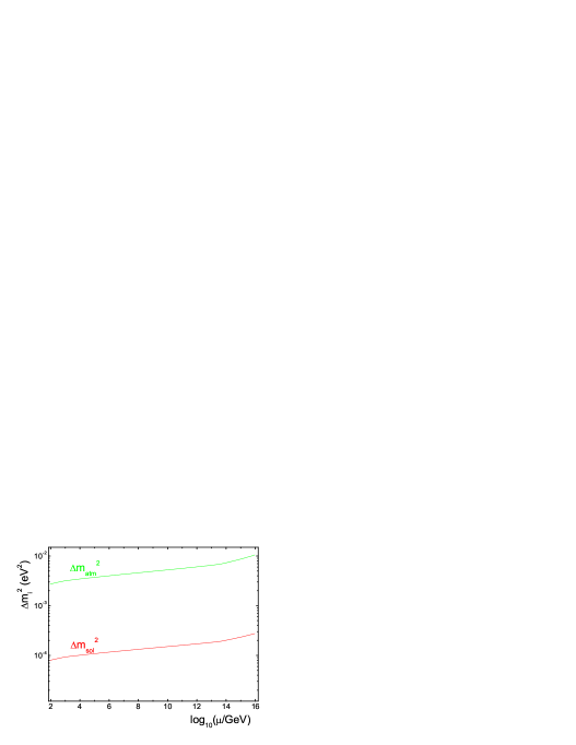
Figure 6: Running of $\Delta m^{2}_{sol}$ and $\Delta m^{2}_{atm}$.

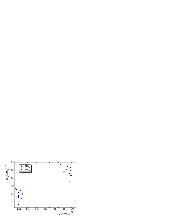
Figure 7: $\Delta m^{2}_{12}$ and $\Delta m^{2}_{23}$ at $M_{Z}$ and at $M_{G}$.

IV Conclusions

In this work, we studied the running of neutrino masses and mixing angles in a supersymmetric string-inspired SU$(4)\times$SU$(2)_{L}\times$SU$(2)_{R}\times$U$(1)_{X}$ model. An accurate description of the low energy neutrino data forced us to introduce two singlets charged under the $U(1)_{X}$, leading to two expansion parameters. The mass matrices are then constructed in terms of three expansion parameters

$$\epsilon\equiv\frac{\langle\phi\rangle}{M_{U}},\ \ \epsilon^{\prime}\equiv\frac{\langle H\bar{H}\rangle}{M_{U}^{2}},\ \ \epsilon^{\prime\prime}\equiv\frac{\langle\chi\rangle}{M_{U}},$$ (28)

where $\phi$ and $\chi$ are singlets and $H$, $\bar{H}$ the SU$(4)\times$SU$(2)_{R}$-breaking Higgses. The model is simplified by the fractional U$(1)_{X}$ charges of $H$ and $\chi$, which ensure that the parameter $\epsilon^{\prime\prime}$ only appears as a prefactor to the heavy Majorana neutrino masses.

The expansion parameter arising from the Higgs v.e.v.’s defines the ratio of the $SU(4)$ breaking scale $M_{G}$ to the unification scale $M_{U}$: we performed a renormalization group analysis of gauge couplings under this constraint and found successful unification with the addition of extra states usually present in a string spectrum.

Assuming that only the third generation of quarks and charged leptons acquire masses at tree level and under a specific choice of $U(1)_{X}$ charges as well as Clebsch factors, we examined the implications for the light neutrino masses resulting from the see-saw formula. We found that the light neutrino mass spectrum is hierarchical and that the mass hierarchy tends to be larger at the GUT scale than at $M_{Z}$ due the renormalization group running. The solar mixing angle $\theta_{12}$ is stable under RG evolution while larger renormalization effects are found for the atmospheric mixing angle $\theta_{23}$ and $\theta_{13}$, always with their values at $M_{Z}$ in agreement with experiment.

References

- (1) J. N. Bahcall, M. C. Gonzalez-Garcia and C. Peña-Garay, JHEP 0408, 016 (2004) [hep-ph/0406294]; G. Altarelli, hep-ph/0405182; M. Maltoni, T. Schwetz, M. A. Tortola and J. W. F. Valle, New J. Phys. 6, 122 (2004) [hep-ph/0405172]; M. C. Gonzalez-Garcia and C. Pena-Garay, Phys. Rev. D 68, 093003 (2003) [hep-ph/0306001].
- (2) J. C. Pati and A. Salam, Phys. Rev. D 10, 275 (1974). R. N. Mohapatra and J. C. Pati, Phys. Rev. D 11, 2558 (1975).
- (3) S. T. Petcov and A. Y. Smirnov, Phys. Lett. B 322, 109 (1994).
- (4) H. Minakata and A. Y. Smirnov, Phys. Rev. D 70, 073009 (2004) [hep-ph/0405088]. For a recent review see H. Minakata, hep-ph/0505262.
- (5) S. Antusch, S. F. King and R. N. Mohapatra, hep-ph/0504007; P. H. Frampton and R. N. Mohapatra, JHEP 0501, 025 (2005) [hep-ph/0407139]. For a review see R. N. Mohapatra and A. Y. Smirnov, hep-ph/0603118.
- (6) S. T. Petcov, Phys. Lett. B 110, 245 (1982); T. Fukuyama and H. Nishiura, hep-ph/9702253; R. Barbieri et al., JHEP 9812, 017 (1998); A. S. Joshipura and S. D. Rindani, Eur. Phys. J. C 14, 85 (2000); R. N. Mohapatra, A. Perez-Lorenzana and C. A. de Sousa Pires, Phys. Lett. B 474, 355 (2000); Q. Shafi and Z. Tavartkiladze, Phys. Lett. B 482, 145 (2000). L. Lavoura, Phys. Rev. D 62, 093011 (2000); W. Grimus and L. Lavoura, Phys. Rev. D 62, 093012 (2000); T. Kitabayashi and M. Yasue, Phys. Rev. D 63, 095002 (2001); K. S. Babu and R. N. Mohapatra, Phys. Lett. B 532, 77 (2002); R. N. Mohapatra, S. Nasri and H. B. Yu, hep-ph/0603020; J. C. Gomez-Izquierdo and A. Perez-Lorenzana, hep-ph/0601223.
- (7) G. K. Leontaris, J. Rizos and A. Psallidas, Phys. Lett. B 597, 182 (2004) [hep-ph/0404129]; G. K. Leontaris, A. Psallidas and N. D. Vlachos, hep-ph/0511327; see also K. L. McDonald and B. H. J. McKellar, hep-ph/0603129.
- (8) T. Fukuyama and N. Okada, JHEP 0211, 011 (2002); S. Antusch, J. Kersten, M. Lindner, M. Ratz and M. A. Schmidt, JHEP 0503, 024 (2005) [hep-ph/0501272].
- (9) J. w. Mei, Phys. Rev. D 71, 073012 (2005) [hep-ph/0502015].
- (10) J. Ellis, A. Hektor, M. Kadastik, K. Kannike and M. Raidal, hep-ph/0506122.
- (11) T. Dent, G. Leontaris and J. Rizos, Phys. Lett. B 605, 399 (2005) [hep-ph/0407151].
- (12) I. Antoniadis and G. K. Leontaris, Phys. Lett. B 216, 333 (1989), and Phys. Lett. B 245, 161 (1990); G. K. Leontaris and J. Rizos, Nucl. Phys. B 554, 3 (1999).
- (13) B. C. Allanach and S. F. King, Nucl. Phys. B 459, 75 (1996); J. C. Pati, Nucl. Phys. Proc. Suppl. 137, 127 (2004) [hep-ph/0407220]; J. C. Pati, hep-ph/0507307.
- (14) B. C. Allanach, S. F. King, G. K. Leontaris and S. Lola, Phys. Rev. D 56, 2632 (1997).
- (15) B. C. Allanach and S. F. King, Phys. Lett. B 353 477 (1995).
- (16) G. K. Leontaris and N. D. Tracas, Phys. Lett. B 372 219 (1996).
- (17) S. Eidelman et al., Phys. Lett. B592, 1 (2004).
- (18) N. Irges, S. Lavignac and P. Ramond, Phys. Rev. D 58, 035003 (1998); G. Altarelli and F. Feruglio, Phys. Lett. B 439, 112 (1998); J. R. Ellis, G. K. Leontaris, S. Lola and D. V. Nanopoulos, Eur. Phys. J. C 9, 389 (1999); G. K. Leontaris and J. Rizos, Nucl. Phys. B 567, 32 (2000).
- (19) P. H. Chankowski and Z. Pluciennik, Phys. Lett. B 316, 312 (1993); K. S. Babu, C. N. Leung and J. T. Pantaleone, Phys. Lett. B 319, 191 (1993); N. Haba, N. Okamura and M. Sugiura, Prog. Theor. Phys. 103, 367 (2000); N. Haba, Y. Matsui, N. Okamura and M. Sugiura, Eur. Phys. J. C 10, 677 (1999); N. Haba and N. Okamura, Eur. Phys. J. C 14, 347 (2000); S. Antusch, M. Drees, J. Kersten, M. Lindner and M. Ratz, Phys. Lett. B 519, 238 (2001), and Phys. Lett. B 525, 130 (2002).
- (20) S. Antusch, J. Kersten, M. Lindner and M. Ratz, Phys. Lett. B 538, 87 (2002) [hep-ph/0203233]. J. A. Casas, J. R. Espinosa, A. Ibarra and I. Navarro, Nucl. Phys. B 573, 652 (2000); P. H. Chankowski, W. Krolikowski and S. Pokorski, Phys. Lett. B 473, 109 (2000).
- (21) S. Antusch, J. Kersten, M. Lindner and M. Ratz, Nucl. Phys. B 674, 401 (2003) [hep-ph/0305273].
- (22) B. Grzadkowski and M. Lindner, Phys. Lett. B 193, 71 (1987); B. Grzadkowski, M. Lindner, and S. Theisen, Phys. Lett. B 198, 64 (1987); J. A. Casas, J. R. Espinosa, A. Ibarra, and I. Navarro, Nucl. Phys. B 556, 3 (1999), and Nucl. Phys. B 569, 82 (2000).
- (23) J. R. Ellis and S. Lola, Phys. Lett. B 458, 310 (1999) R. Barbieri, G. G. Ross and A. Strumia, JHEP 9910, 020 (1999); N. Haba, Y. Matsui, N. Okamura and M. Sugiura, Prog. Theor. Phys. 103, 145 (2000).
- (24) M. Dine, N. Seiberg and E. Witten, Nucl. Phys. B 289 589 (1987).
- (25) For a recent review see S. T. Petcov, hep-ph/0504166.
- (26) H. V. Klapdor-Kleingrothaus et al., Eur. Phys. J. A 12, 147 (2001).
- (27) S. Choubey and W. Rodejohann, Phys. Rev. D 72, 033016 (2005) [hep-ph/0506102].