Neutrino masses in the Lepton Number Violating MSSM

Abstract:

We consider the most general supersymmetric model with minimal particle content and an additional discrete ${\cal Z}_{3}$ symmetry (instead of R-parity), which allows lepton number violating terms and results in non-zero Majorana neutrino masses. We investigate whether the currently measured values for lepton masses and mixing can be reproduced. We set up a framework in which Lagrangian parameters can be initialised without recourse to assumptions concerning trilinear or bilinear superpotential terms, CP-conservation or intergenerational mixing and analyse in detail the one loop corrections to the neutrino masses. We present scenarios in which the experimental data are reproduced and show the effect varying lepton number violating couplings has on the predicted atmospheric and solar mass² differences. We find that with bilinear lepton number violating couplings in the superpotential of the order 1 MeV the atmospheric mass scale can be reproduced. Certain trilinear superpotential couplings, usually, of the order of the electron Yukawa coupling can give rise to either atmospheric or solar mass scales and bilinear supersymmetry breaking terms of the order 0.1 $\textup{GeV}^{2}$ can set the solar mass scale. Further details of our calculation, Lagrangian, Feynman rules and relevant generic loop diagrams, are presented in three Appendices.

1 Introduction

Once one allows for R-parity [1] violation in the Minimal Supersymmetric Standard Model (MSSM) there is an embarrassingly large class of possible models. Building on the seminal paper of Ibanez and Ross [2], it has been shown that there are three preferred ${\cal Z}_{N}$ symmetries which can be imposed when constructing the MSSM with minimal content of particle fields [3]: one is the standard R-parity under which the Standard Model particles are R-parity even while their superpartners are R-parity odd, the second is a unique, ${\cal Z}_{3}$ symmetry which results in the MSSM with lepton number violation; denoted here as ( /L-MSSM ) and the third is a ${\cal Z}_{6}$ symmetry refered to as proton hexality. The former guarantees a stable lightest supersymmetric particle and thus missing energy at colliders, the ${\cal Z}_{3}$ and ${\cal Z}_{6}$ lead to proton stability together with neutrino flavour changing phenomena and masses. In this paper we want to investigate in detail neutrino masses and mixings in the /L-MSSM motivated from the current observations of neutrino flavour metamorphosis and proton stability [4].

In the /L-MSSM a single neutrino mass arises at tree level due to the mixing between neutrinos, gauginos and higgsinos [5, 6, 7, 8]. This tree level mass is proportional to the bilinear lepton number violating superpotential parameter, $\mu_{i}$, squared, which is assumed to be of order of ${\rm MeV}$, and is suppressed by the “TeV” supersymmetry breaking gaugino masses, resulting in a low energy see-saw mechanism with light neutrino and heavy neutralino masses. The other two neutrino masses arise from quantum loop corrections made up from lepton number violating superpotential or supersymmetry breaking vertices. We shall refer to these neutrinos with the term “massless neutrinos”.

Calculations for neutrino masses in the /L-MSSM have been addressed many times in the literature. The tree level set-up of the model was first given in [5], and details worked out later in [6, 7, 8]. Calculations of the one-loop neutrino masses including only the bilinear superpotential term are given in [11, 12, 13, 14, 15]. Corrections involving the trilinear superpotential Yukawa couplings $\lambda,\lambda^{\prime}$ considered mostly in the mass insertion approximation [17, 18, 19, 20] and under the assumption of CP-conservation and flavour diagonal soft SUSY breaking terms. Renormalization group induced corrections to neutrino masses have been studied in [21, 22, 23]. There is of course a vast number of articles using these calculations, or simplified versions of them, in order to describe the solar and atmospheric neutrino puzzles [24, 26, 27, 28, 29, 30, 31, 32, 33, 34].

In this work, we calculate the complete set of the one-loop corrections to the massless neutrinos without resorting to approximations about CP-conservation or bilinear superpotential operator dominance. The outline of our paper is as follows : in section 2 we show how to define the Lagrangian parameters in the fermion sector of the theory, by starting out with physical input parameters like the lepton masses and mixing angles. In section 3 we describe our renormalization procedure and present analytical results for the one-loop corrections together with approximate formulas (if necessary) for individual diagrams. We compare with the current literature. In section 4 we present numerical results for the size of the input parameters when these account for the neutrino experimental data, and in section 5 draw our conclusions. Finally, in three Appendices, we set out our notation, in Appendix A, the Lagrangian and the mass terms, and present the relevant Feynman rules in Appendix B. Furthermore, in Appendix C we present a pedagogical brief introduction to the Weyl spinor calculation that are employed throughout this paper and present general one-loop self energy corrections that are employed in this paper and can be used elsewhere.

The Fortran-code for calculating the neutrino masses used in this article has been made publicly available. It can be used in adding additional constraints when other /L-MSSM processes are studied.

2 Fermion masses and mixings in /L-MSSM 

Fermion masses and couplings of the general /L-MSSM are defined by the superpotential of the model, vacuum expectation values (vevs) of the neutral scalar fields and the soft supersymmetry breaking gaugino masses. The most general superpotential takes the form

$${\cal W}_{\rm~{}{/}L-MSSM~{}}=\epsilon_{ab}\left(\frac{1}{2}\lambda_{\alpha\beta k}{\cal L}_{\alpha}^{a}{\cal L}_{\beta}^{b}\bar{E}_{k}\>+\>\lambda^{\prime}_{\alpha jk}{\cal L}_{\alpha}^{a}Q_{j}^{b,x}\bar{D}_{k,x}\>+\>(Y_{U})_{jk}Q_{j}^{a,x}H_{2}^{b}\bar{U}_{k,x}\>-\>\mu_{\alpha}{\cal L}_{\alpha}^{a}H_{2}^{b}\right),$$

(1)

where $Q_{i}^{a\,x},\;{\bar{D}}_{i}^{x},\;{\bar{U}}_{i}^{x},\;{\cal L}_{i}^{a},\;{\bar{E}}_{i},\;H_{1}^{a},\;H_{2}^{a}$ are the chiral superfield particle content, $i=1,2,3$ is a generation index, $x=1,2,3$ and $a=1,2$ are $SU(3)$ and $SU(2)$ gauge indices, respectively. The simple form of (1) results when combining the chiral doublet superfields with common hypercharge $Y=-\frac{1}{2}$ into ${\cal L}^{a}_{\alpha=0,\ldots,3}=(H_{1}^{a},\,L_{i=1,2,3}^{a})$. $\mu_{\alpha}$ is the generalized dimensionful $\mu$-parameter, with $\mu_{0}$ and $\mu_{i},i=1,...3$ the lepton number conserving and violating parts respectively, and $\lambda_{\alpha\beta k},\,\lambda^{\prime}_{\alpha jk},(Y_{U})_{ij}$ are Yukawa matrices with $\epsilon_{ab}$ being the totally anti-symmetric tensor $\epsilon_{12}=+1$.

Physical masses of the fermion fields depend on appropriate $\lambda,\lambda^{\prime},\mu$ and $Y_{U}$ couplings multiplied by the vevs of the neutral scalar fields. As it has been shown in [36, 35], by unitary rotation in the 4-dimensional space of the neutral scalar components of $\mathcal{L}_{\alpha}$, it is possible to set three of the four vacuum expectation values of the $\mathcal{L}_{\alpha}$ fields to zero, leaving two real non-zero vevs in the neutral scalar sector and, simultaneously, significantly simplifying its structure. It is convenient to apply such a transformation not just to scalars, but to the whole chiral superfield,

$$\mathcal{L}_{\alpha}=U_{\alpha\beta}\mathcal{L}_{\beta}^{{}^{\prime}}\;,$$ (2)

and redefine the Lagrangian parameters to absorb the matrix $\bf U$ in Eq. (2) such that it does not appear explicitly in the Lagrangian,

$$\tilde{\lambda}_{\gamma\delta j} = \lambda^{\phantom{*}}_{\alpha\beta j}U_{\alpha\gamma}U_{\beta\delta}\;,$$

$$\tilde{\lambda^{\prime}}_{\gamma ij} = {\lambda^{\prime}}^{\phantom{*}}_{\!\!\alpha ij}U_{\alpha\gamma}\;,$$ (3)

$$\tilde{\mu}_{\gamma} = \mu_{\alpha}U_{\alpha\gamma}\;.$$

The tildes and primes on the fields are then dropped.

In a standard way, both isospin components of $Q$ superfield and of $\bar{U}$, $\bar{D}$ superfields can each be redefined by a unitary rotation in the flavour space. As such, it is possible to diagonalise the Yukawa couplings ${\bf(Y_{D})}$, $\bf\left(Y_{U}\right)^{\phantom{*}}$ (note that ${\bf(Y_{D})}\equiv\lambda^{\prime}_{0ij}$ in the basis with two non-vanishing scalar vevs) and absorb the rotation matrices in field redefinitions such that they do not appear explicitly in the Lagrangian, apart from a specific combination of rotation matrices which appear in the gauge and Higgs charged currents which is identified as the CKM matrix. In this basis, it is clear how to initialise the Lagrangian parameters, as the diagonal values are then proportional to the measured values for the up- and down-type quarks. For more details concerning this point the reader should consult Appendix A.

In the lepton sector, however, the same approach cannot be adopted for two reasons. Firstly, even with a diagonal Yukawa matrix, the charged lepton masses are given by three eigenvalues of the larger $(5\times 5)$ mass matrix which includes mixing between the charged fermionic components of the $\mathcal{L}$, $\bar{E}$ and the charged gauginos and higgsinos. Thus, the diagonal entries in the Yukawa matrix would not correspond exactly to the masses of the physical mass eigenstates which describe the charged leptons. Secondly, the $\mathcal{L}$-basis has already been fixed by the property that three neutral scalar vevs should be zero, so we are not free to absorb a rotation matrix.

Still, there is some freedom remaining due to the fact that the $\bar{E}$-base has not, as yet, been fixed. Flavour rotation in the $\bar{E}$-space can be used to remove some of the unphysical degrees of freedom in ${\bf Y_{L}}\equiv\lambda_{0ij}$ coupling. As every general, complex matrix, $\lambda_{0ij}$ can be uniquely decomposed (polar decomposition theorem [38]) into a product of positive semi-definite Hermitian matrix $\hat{\lambda}_{0}$ and unitary matrix $V_{E}$ :

$$\lambda_{0ij}\ =\ \hat{\lambda}_{0ik}\>(V_{E})_{kj}\;,$$ (4)

$V_{E}$ can be then adsorbed in the chiral superfield $\bar{E}$ redefinition and the ‘hat’ over $\lambda$ is dropped.

After all the transformations described above, we arrived to the form of the superpotential (1) where ${\bf(Y_{D})}_{ij}=\lambda^{\prime}_{0ij}$ and ${\bf(Y_{U})}_{ij}$ are flavour-diagonal and ${\bf(Y_{L})}_{ij}=\lambda_{0ij}$ is hermitian. Other coupling constants are free and, in general, complex parameters.

2.1 Block Diagonalising

In the following sections we outline the procedure by which the parameters of the general hermitian matrix ${\bf(Y_{L})}_{ij}$ can be initialised such that the correct values are obtained for the charged lepton masses and the MNS mixing matrix [39]. In order to do that, it will be convenient to diagonalise the neutralino-neutrino and chargino-charged lepton mass matrices in two stages. First an approximate, unitary or biunitary transformation will result in matrices in block diagonal form; the standard model and supersymmetric fermion masses being split into separate blocks. Then, a second transformation will diagonalize the blocks.

The block diagonalisation can be performed for any complex matrix. Every general matrix $M$ can be diagonalised by two unitary matrices $V,U$:

$$V^{\dagger}MU=\hat{M}=\textup{diag}(m_{1},m_{2},\cdots,m_{n})=\left(\begin{array}[]{cc}M_{1}&0\\ 0&M_{2}\\ \end{array}\right)\;,$$ (5)

where $m_{i}^{2}$ are eigenvalues of $MM^{\dagger}$ and $M_{1},M_{2}$ are two diagonal sub-matrices of a chosen size. Hence, one can always rewrite $M$ in the form

$$M=V\hat{M}U^{\dagger}=VA^{\dagger}A\hat{M}B^{\dagger}BU^{\dagger}\;,$$ (6)

where $A$ and $B$ are some unitary matrices of the form

$$\begin{array}[]{cc}A=\left(\begin{array}[]{cc}A_{1}&0\\ 0&A_{2}\\ \end{array}\right)\;,\qquad B=\left(\begin{array}[]{cc}B_{1}&0\\ 0&B_{2}\\ \end{array}\right)\end{array}\;,$$ (7)

with sub-matrices $A_{1,2},B_{1,2}$ which are also unitary. Thus we can write

$$M=QM_{B}P^{\dagger}\;,$$ (8)

where

$$M_{B}=A\hat{M}B^{\dagger}=\left(\begin{array}[]{cc}A_{1}M_{1}B_{1}^{\dagger}&0\\ 0&A_{2}M_{2}B_{2}^{\dagger}\end{array}\right)\;,$$ (9)

is block diagonal in form and $Q=VA{{}^{\dagger}}$, $P=UB^{\dagger}$. Of course, $M_{B}$ is not uniquely defined.

Block diagonalisation is particularly useful in case of hierarchical matrices, when one can find analytical approximate formulae for $P,Q$ matrices in eq.(8). Consider for example a hermitian matrix (other cases can be considered analogously) of the form:

$$M=\left(\begin{array}[]{cc}m_{A}&m_{B}\\ m_{B}^{\dagger}&m_{C}\end{array}\right)\;,$$ (12)

where $m_{A}=m_{A}^{\dagger}$, $m_{C}=m_{C}^{\dagger}$ and $||m_{A}||\gg||m_{B}||,||m_{C}||$. In such case, the approximately (up to the terms ${\cal O}(||m_{B,C}||^{2}/||m_{A}||^{2})$) unitary matrix $U$,

$$U=\left(\begin{array}[]{cc}1&-(m_{A})^{-1}m_{B}\\ m_{B}^{\dagger}(m_{A})^{-1}&1\end{array}\right)\;,$$ (15)

transforms $M$ into approximately block-diagonal form:

$$U^{\dagger}MU = \left(\begin{array}[]{cc}m_{A}{+}(m_{A})^{-1}m_{B}m_{B}^{\dagger}+m_{B}m_{B}^{\dagger}(m_{A})^{-1}&(m_{A})^{-1}m_{B}m_{C}\\ m_{C}^{\dagger}m_{B}^{\dagger}(m_{A})^{-1}&m_{C}-m_{B}^{\dagger}(m_{A})^{-1}m_{B}\end{array}\right)+{\cal O}\left(||m_{B,C}||^{3}\over||m_{A}||^{2}\right)$$ (18)

$$\approx \left(\begin{array}[]{cc}m_{A}&0\\ 0&m_{C}-m_{B}^{\dagger}(m_{A})^{-1}m_{B}\end{array}\right)+{\cal O}\left({||m_{B,C}||^{2}\over||m_{A}||}\right)\;.$$ (21)

We kept explicitly the ${\cal O}\left({||m_{B,C}||^{2}\over||m_{A}||}\right)$ term in (22) element of block-diagonalised form of $M$ as in many models $m_{C}\equiv 0$ and in this case it will be the only term which survives (the see-saw mechanism [40, 41] for neutrino masses being the most famous example of this hierarchical structure).

As a next step one needs to find matrices that diagonalise the sub-blocks in eq.(21). We employ this method in the next sections where we present explicit perturbative ($1_{\mathrm{st}}$ order) results for analogs of the matrices $Q$ and $P$ in Eq. (8), in both neutral and charged fermion masses in the /L-MSSM . In passing that, although we use only the approximate analytical expressions for the see-saw type expansions above, in our numerical predictions we perform exact block diagonalization, iteratively finding the correct, and strictly unitary, matrices $P,Q$ of eq.(8).

2.2 Fermion masses and mixing

In the following section we shall present the tree level phenomena of the fermion sector in the /L-MSSM . We consider in turn, the neutral and charged fermion sectors and the patterns of the mass matrices. We consider the tree level eigenvalues, particularly for the neutral sector and the approximate block diagonalisation of the matrices. In section 2.3, we use the approximate block diagonalisation to consider the way in which the MNS matrix appears in this model, as it is now a sub-block of a larger unitary matrix, the MNS matrix itself is not generally unitary. This analysis is then used to ensure the correct low energy parameters are reproduced, despite mixing between the leptons and heavy fermion fields.

In section 3 we consider the effect of radiative corrections at the order of one-loop. After setting out the renormalisation framework, we present in turn various loop diagrams and highlight the important contributions. The full numerical analysis has been completed, however approximate expression are presented for each contribution which demonstrate from where the important effects arise. We will consider the case where the tree-level effect dominates and gives rise to the larger, atmospheric mass squared difference, in which case the solar mass squared difference is generated by the loop effects. We also show that it is possible for loop effects to be greater than the tree level affects, in which case both mass squared differences are generated at the level of one-loop.

2.2.1 Neutral fermion sector

In the lepton number violating extension of the minimal supersymmetric standard model ( /L-MSSM ) the neutrinos ($\nu_{L1,2,3}$), neutral higgsinos ($\nu_{L0}$ and $\tilde{h}_{2}^{0}$)and neutral colourless gauginos ($\widetilde{W}_{0}$ and $\widetilde{B}$) mix. To transform the fields into the mass basis, the $7\times 7$ neutralino mass matrix must be diagonalised. In the interaction basis,

$$\mathcal{L}\supset-\frac{1}{2}\left(\begin{array}[]{cccc}-i\widetilde{B},&-i\widetilde{W}_{0},&\tilde{h}_{2}^{0},&\nu_{L\alpha}\\ \end{array}\right)\mathcal{M}_{N}\left(\begin{array}[]{c}-i\widetilde{B}\\ -i\widetilde{W}_{0}\\ \tilde{h}_{2}^{0}\\ \nu_{L\beta}\\ \end{array}\right)\ +\ {\rm H.c}\;,$$ (22)

where the full $7\times 7$ mass matrix reads

$$\mathcal{M}_{N}=\left(\begin{array}[]{cc}M_{N\,\tiny{4\times 4}}&d_{N\,\tiny{4\times 3}}\\ d^{T}_{N\,\tiny{3\times 4}}&0_{\tiny{3\times 3}}\end{array}\right)\;,$$ (23)

and the sub-blocks are, in the basis $(-i\widetilde{B},-i\widetilde{W}_{0},\tilde{h}_{2}^{0},\nu_{L\alpha}\equiv\tilde{h}^{0}_{1},\nu_{i})$ [35]

$$M_{N\,\tiny{4\times 4}}=\left(\begin{array}[]{cccc}M_{1}&0&\frac{gv_{u}}{2}&-\frac{gv_{d}}{2}\\ 0&M_{2}&-\frac{g_{2}v_{u}}{2}&\frac{g_{2}v_{d}}{2}\\ \frac{gv_{u}}{2}&-\frac{g_{2}v_{u}}{2}&0&-\mu_{0}\\ -\frac{gv_{d}}{2}&\frac{g_{2}v_{d}}{2}&-\mu_{0}&0\\ \end{array}\right)\;,$$ (24)

and

$$d_{N\tiny{4\times 3}}=\left(\begin{array}[]{cccc}0&0&0\\ 0&0&0\\ -\mu_{1}&-\mu_{2}&-\mu_{3}\\ 0&0&0\\ \end{array}\right)\;.$$ (25)

There is no quantum number to differentiate between neutralinos and neutrinos, the states of definite mass do not have definite lepton number and, as such, there is no reason to think of neutrinos and neutralinos separately. However, for realistic values of parameters, four of the mass eigenstates are heavy and three are very light, so it is convenient to refer to them as to neutralinos and neutrinos, respectively. In addition to this, it can be seen that the mixing is sufficiently small that these three light neutral states are the states which dominantly appear in the decay of the W boson to charged leptons, differentiating between the eigenstates we refer to as neutrinos from those we refer to as neutralinos.

The matrix,$Z_{N}$, which rotates the fields in (22) from the interaction basis to the mass eigenstate basis is given by

$$\left(\begin{array}[]{c}-i\widetilde{B}\\ -i\widetilde{W}^{0}\\ \tilde{h}_{2}^{0}\\ \nu_{L\alpha}\end{array}\right)=Z_{N}\left(\begin{array}[]{c}\kappa^{0}_{1}\\ \vdots\\ \kappa^{0}_{7}\end{array}\right)\;.$$ (26)

where $\kappa^{0}_{1,\ldots,7}$ are seven neutral two component spinors.

The matrix $\mathcal{M}_{N}$, as it has been split in eq.(23), contains block diagonal terms that conserve lepton number and off diagonal blocks which violate lepton number. The latter are expected to be very small, as they are strongly constrained by the bounds on neutrino masses or other lepton number violating processes. Thus, one can use the block diagonalization procedure of section 2.1 and, neglecting terms of the order $d_{N}^{2}\over M_{N}^{2}$ and assume $Z_{N}$ to be of the form

$$Z_{N}=\left(\begin{array}[]{cc}1&-M_{N}^{-1}d_{N}\\ {d_{N}^{\dagger}}M_{N}^{{\dagger}-1}&1\end{array}\right)\left(\begin{array}[]{cc}{\cal Z}_{N}&0\\ 0&{\cal Z}_{\nu}\end{array}\right)\;.$$ (27)

The first matrix on the RHS of eq.(27) which is the analog of the matrix $Q^{\dagger}$ in (8) block diagonalises the neutrino-neutralino mass matrix:

$$\left(\begin{array}[]{cc}1&M_{N}^{{\dagger}-1}{{d_{N}^{*}}}\\ -d_{N}^{T}M_{N}^{-1}&1\end{array}\right)\mathcal{M}_{N}\left(\begin{array}[]{cc}1&-M_{N}^{-1}d_{N}\\ {{d_{N}^{\dagger}}}M_{N}^{{\dagger}-1}&1\end{array}\right)\approx\left(\begin{array}[]{cc}M_{N\,\tiny{4\times 4}}&0\\ 0&m_{\nu\,\tiny{3\times 3}}^{eff}\end{array}\right)\;,$$ (34)

where the “TeV” see-saw suppressed effective $3\times 3$ neutrino mass matrix is given by [6, 7, 8]

$$m^{eff}_{\nu}=-d_{N}^{T}M_{N}^{-1}d_{N}={v_{d}^{2}(M_{1}g_{2}^{2}+M_{2}g^{2})\over 4\textup{Det}[M_{N}]}\left(\begin{array}[]{ccc}\mu_{1}^{2}&\mu_{1}\mu_{2}&\mu_{1}\mu_{3}\\ \mu_{1}\mu_{2}&\mu_{2}^{2}&\mu_{2}\mu_{3}\\ \mu_{1}\mu_{3}&\mu_{2}\mu_{3}&\mu_{3}^{2}\\ \end{array}\right)\;.$$ (38)

Physical neutralino masses and mixing matrix ${\cal Z}_{N}$ can be found in a standard manner by numerical diagonalization of the matrix $M_{N}$. Diagonalization on $m_{\nu}^{eff}$ can be easily done analytically, leading to two massless and one massive neutrino, with its mass given by:

$$m_{\nu}^{tree}=\left|{v_{d}^{2}(M_{1}g_{2}^{2}+M_{2}g^{2})\over 4\textup{Det}[M_{N}]}\right|(|\mu_{1}|^{2}+|\mu_{2}|^{2}+|\mu_{3}|^{2})\;,$$ (39)

and the mixing matrix ${\cal Z}_{\nu}$ is

$${\cal Z}_{\nu}=\left(\begin{array}[]{ccc}\frac{|\mu_{2}|}{\sqrt{|\mu_{1}|^{2}+|\mu_{2}|^{2}}}&\frac{|\mu_{1}||\mu_{3}|}{\sqrt{|\mu_{1}|^{2}+|\mu_{2}|^{2}}\sqrt{|\mu_{1}|^{2}+|\mu_{2}|^{2}+|\mu_{3}|^{2}}}&\frac{|\mu_{1}|}{\sqrt{|\mu_{1}|^{2}+|\mu_{2}|^{2}+|\mu_{3}|^{2}}}\\ \frac{-|\mu_{2}|\mu_{1}}{\mu_{2}\sqrt{|\mu_{1}|^{2}+|\mu_{2}|^{2}}}&\frac{\mu_{1}\mu^{*}_{2}|\mu_{3}|}{|\mu_{1}|\sqrt{|\mu_{1}|^{2}+|\mu_{2}|^{2}}\sqrt{|\mu_{1}|^{2}+|\mu_{2}|^{2}+|\mu_{3}|^{2}}}&\frac{|\mu_{1}|\mu^{*}_{2}}{\mu^{*}_{1}\sqrt{|\mu_{1}|^{2}+|\mu_{2}|^{2}+|\mu_{3}|^{2}}}\\ 0&-\frac{\mu_{1}|\mu_{3}|\sqrt{|\mu_{1}|^{2}+|\mu_{2}|^{2}}}{\mu_{3}|\mu_{1}|\sqrt{|\mu_{1}|^{2}+|\mu_{2}|^{2}+|\mu_{3}|^{2}}}&\frac{|\mu_{1}|\mu^{*}_{3}}{\mu^{*}_{1}\sqrt{|\mu_{1}|^{2}+|\mu_{2}|^{2}+|\mu_{3}|^{2}}}\\ \end{array}\right)\left(\begin{array}[]{c|c}X_{2\times 2}&0\\ \hline\cr 0&1\end{array}\right)\;,$$ (45)

(46)

where $X_{2\times 2}$ is an $SU(2)$ rotation. At tree level, the five massive eigenstates are unambiguously defined by diagonalising the mass matrix. The two massless eigenstates, due to the fact that they are degenerate in mass, are not fully defined. The eigenstates are chosen to be orthogonal, but it is still possible to perform a rotation on the eigenstates. As such, statements about the lightest neutrinos, $\nu_{1,2}$, are basis dependent. Because of this, the one loop contributions to $\hat{{\cal M}}_{N\,pq}$ are also basis dependent. By choosing a different linear superposition of the tree level eigenstates, the one-loop contributions to the $2\times 2$ sub-lock $\hat{{\cal M}}_{N\,(5,6)(5,6)}$ referring to the massless neutrinos would be redistributed between themselves. This freedom of basis choice is only present at tree level and is not physical. Thus, we start from $X_{2\times 2}=1_{2\times 2}$ and after calculating the radiative corrections to the neutralino-neutrino mass matrix we adjust $X_{2\times 2}$ such that the off-diagonal one-loop contribution $\delta M_{N\,56}$ is approximately zero (this can be done iteratively). As such the effect of rediagonalising the neutrino sector after loop corrections are added is small. As we discuss in section 2.3, choosing the basis in this manner helps also to define the lepton Yukawa couplings in terms of measured quantities like lepton masses and the $U_{MNS}$ mixing matrix.

The result that two of the neutrino masses vanish at the tree level is not the effect of the approximations made [6, 7, 8]. The explicit calculation of the secular equation for the full neutralino-neutrino mass matrix $\mathcal{M}_{N}$, results in

$$\det(\mathcal{M}_{N}-\lambda) = -\lambda^{2}\left[\lambda\det(M_{N}{-\lambda})\right.$$

$$- \left.(\mu_{1}^{2}+\mu_{2}^{2}+\mu_{3}^{2})\left(\lambda(M_{1}-\lambda)(M_{2}-\lambda)+{g_{2}^{2}v_{d}^{2}\over{4}}(M_{1}-\lambda)+{g^{2}v_{d}^{2}\over{4}}(M_{2}-\lambda)\right)\right]\;.$$

Hence, $\mathcal{M}_{N}$ always has at least two zero modes. This can be seen directly, by noting that the final three columns of the $7\times 7$ mass matrix are proportional to each other.

Finally, the physical eigenstates of neutralinos and neutrinos are approximately given by, respectively:

$${\cal Z}_{N}\left(\begin{array}[]{c}\kappa^{0}_{1}\\ \kappa^{0}_{2}\\ \kappa^{0}_{3}\\ \kappa^{0}_{4}\end{array}\right)=\left(\begin{array}[]{c}-i\widetilde{B}\\ -i\widetilde{W}_{0}\\ \tilde{h}_{2}^{0}\\ \nu_{L0}\end{array}\right)+M_{N}^{-1}d_{N}\nu_{Li}\;,$$ (48)

and

$${\cal Z}_{\nu}\left(\begin{array}[]{c}\kappa^{0}_{5}\\ \kappa^{0}_{6}\\ \kappa^{0}_{7}\end{array}\right)=-d_{N}^{{\dagger}}M_{N}^{{\dagger}-1}\left(\begin{array}[]{c}-i\widetilde{B}\\ -i\widetilde{W}_{0}\\ \tilde{h}_{2}^{0}\\ \nu_{L0}\end{array}\right)+\nu_{Li}\;,$$ (49)

with $\nu_{L0}=\tilde{h}_{1}^{0}$ is the down type Higgsino. For a quick view of definitions see also Appendix A.

2.2.2 Charged fermion sector

In a similar fashion to the neutral sector, charged leptons, gauginos and higgsinos mix. The full $5\times 5$ chargino mass matrix in the basis of Ref. [35] is given by

$$\mathcal{M}_{C}=\left(\begin{array}[]{cc}M_{C\,\tiny{2\times 2}}&0\\ d_{C\,\tiny{3\times 2}}&m_{C\,\tiny{3\times 3}}\end{array}\right)\;,$$ (50)

with the lepton number conserving sub-locks

$$M_{C\,\tiny{2\times 2}}=\left(\begin{array}[]{cc}M_{2}&{g_{2}v_{{u}}\over\sqrt{2}}\\ {g_{2}v_{d}\over\sqrt{2}}&\mu_{{0}}\\ \end{array}\right)\;,\qquad m_{C\,ij}=\frac{v_{d}}{\sqrt{2}}\lambda_{0ij}\;,$$ (51)

and the lepton number violating being

$$d_{C\,\tiny{3\times 2}}=\left(\begin{array}[]{cc}0&\mu_{1}\\ 0&\mu_{2}\\ 0&\mu_{3}\\ \end{array}\right)\;.$$ (52)

The rotation matrices which transform between interaction eigenstates and mass eigenstates are given by

$$\left(\begin{array}[]{c}-i\widetilde{W}^{+}\\ \tilde{h}_{2}^{+}\\ e_{Ri}\end{array}\right)=Z_{+}\left(\begin{array}[]{c}\kappa^{+}_{1}\\ \vdots\\ \kappa^{+}_{5}\end{array}\right)\;,$$ (53)

$$\left(\begin{array}[]{c}-i\widetilde{W}^{-}\\ e_{L\alpha}\end{array}\right)=Z^{*}_{-}\left(\begin{array}[]{c}\kappa^{-}_{1}\\ \vdots\\ \kappa^{-}_{5}\end{array}\right)\;,$$ (59)

and, as such, the mass matrix is diagonalised

$$\hat{\mathcal{M}_{C}}=Z^{\dagger}_{-}\mathcal{M}_{C}Z_{+}\;,$$ (60)

where the ‘hat’ denotes that the matrix is diagonal.

The matrices $Z_{+}$ and $Z_{-}$ can be determined by the requirement that they should diagonalise the Hermitian matrices $\mathcal{M}_{C}^{\dagger}\mathcal{M}_{C}$ and $\mathcal{M}_{C}\mathcal{M}_{C}^{\dagger}$, respectively. The off-diagonal blocks in the latter two combinations are small comparing to the diagonal ones, so one can again use block-diagonalising approximation of section 2.1. Keeping just the leading terms in $1/M_{C}$ expansion, one obtains

$$Z_{-} \approx \left(\begin{array}[]{cc}1&{-}M^{\dagger\,-1}_{C}d^{\dagger}_{C}\\ d_{C}M^{-1}_{C}&1\end{array}\right)\left(\begin{array}[]{cc}{\cal Z}_{-}&0\\ 0&{\cal Z}_{l^{-}}\\ \end{array}\right)\;,$$ (65)

$$Z_{+} \approx \left(\begin{array}[]{cc}{\cal Z}_{+}&0\\ 0&{\cal Z}_{l^{+}}\\ \end{array}\right)\;.$$ (68)

Substitution of (68) in (60) results in the physical effective mass matrix

$$\hat{\mathcal{M}_{C}}=\left(\begin{array}[]{cc}{\cal Z}_{-}^{\dagger}M_{C}{\cal Z}_{+}+{\cal O}\left({d_{C}^{2}\over M_{C}}\right)&{\cal O}\left({d_{C}m_{C}\over M_{C}}\right)\\ {\cal O}\left({d_{C}^{{2}}\over M_{C}^{{1}}}\right)&{\cal Z}_{l^{-}}^{\dagger}m_{C}{\cal Z}_{l^{+}}+{\cal O}\left({d_{C}^{2}m_{C}\over M_{C}^{2}}\right)\\ \end{array}\right)\approx\left(\begin{array}[]{cc}{\cal Z}_{-}^{\dagger}M_{C}{\cal Z}_{+}&0\\ 0&{\cal Z}_{l^{-}}^{\dagger}m_{C}{\cal Z}_{l^{+}}\\ \end{array}\right)\;.$$ (69)

Then the matrices ${\cal Z}_{+},{\cal Z}_{-}$ can be again determined as diagonalising matrices for the $M_{C}^{\dagger}M_{C}$, $M_{C}M_{C}^{\dagger}$ products, with the additional requirement that physical fermion masses are real and positive. Matrix $m_{C}$ in our basis is hermitian and as such ${\cal Z}_{l^{+}}={\cal Z}_{l^{-}}\equiv{\cal Z}_{l}$. Furthermore, physical eigenstates of fermion fields are given by

$${\cal Z}_{+}\left(\begin{array}[]{c}\kappa^{+}_{1}\\ \kappa^{+}_{2}\end{array}\right) \approx \left(\begin{array}[]{c}-i\widetilde{W}^{+}\\ \tilde{h}_{2}^{+}{}\end{array}\right)\;,$$ (74)

$${\cal Z}_{l}\left(\begin{array}[]{c}\kappa^{+}_{3}\\ \kappa^{+}_{4}\\ \kappa^{+}_{5}\end{array}\right) \approx \left(\begin{array}[]{c}e_{R1}\\ e_{R2}\\ e_{R3}\end{array}\right)\;,$$ (81)

and

$${\cal Z}_{-}^{*}\left(\begin{array}[]{c}\kappa^{-}_{1}\\ \kappa^{-}_{2}\end{array}\right) \approx \left(\begin{array}[]{c}-i\widetilde{W}^{-}\\ e_{L0}\end{array}\right)+M_{C}^{-1T}d_{C}^{T}\left(\begin{array}[]{c}e_{L1}\\ e_{L2}\\ e_{L3}\end{array}\right)\;,$$ (89)

$${\cal Z}_{l}^{*}\left(\begin{array}[]{c}\kappa^{-}_{3}\\ \kappa^{-}_{4}\\ \kappa^{-}_{5}\end{array}\right) \approx -d_{C}^{*}M_{C}^{-1*}\left(\begin{array}[]{c}-i\widetilde{W}^{-}\\ e_{L0}\end{array}\right)+\left(\begin{array}[]{c}e_{L1}\\ e_{L2}\\ e_{L3}\end{array}\right)\;.$$ (98)

For a quick view of the full charged fermion mass matrix see Appendix A.

2.3 Constructing the MNS matrix

The lepton mixing matrices appear in the charged current gauge boson vertex. Whereas in the lepton number conserving case the $U_{\rm MNS}$ matrix is a $3\times 3$ matrix describing the mixing of three charged leptons into three neutral leptons, the R-parity violating case has the mixing of five charged fermions into seven neutral fermions, of which the $U_{MNS}$ is a $3\times 3$ sub-matrix, only approximately unitary. Thus,

$${\cal L}\supset\frac{g_{2}}{\sqrt{2}}\>W_{\mu}^{+}\bar{\nu}_{Li}^{\prime}\bar{\sigma}^{\mu}e_{Li}^{\prime}\>+\>{\rm H.c}=\frac{g_{2}}{\sqrt{2}}\>W_{\mu}^{+}\>\bar{\kappa}^{0}_{p}\>\bar{\sigma}^{\mu}\>(U_{\rm MNS})_{pq}\>\kappa^{-}_{q}\>+\>{\rm H.c}\;,$$ (99)

where primes refer to interaction eigenstates, and the MNS matrix,

$$U_{\rm MNS}={\cal Z}_{\nu}^{\dagger}{\cal Z}_{l}^{*}+{\cal O}\left({d_{c}d_{N}\over M_{C}M_{N}}\right)\;,$$ (100)

is defined in terms of the mixing matrices introduced in (46) and below (69).

As the first term in Eq. (100) is unitary, unitarity violation in $U_{\rm MNS}$ is at most of the order of ${d_{c}d_{N}\over M_{C}M_{N}}\sim\frac{m_{\nu}^{\textup{\tiny{tree}}}M_{\textup{\tiny{SUSY}}}}{M_{Z}^{2}}\tan^{2}\beta\sim 10^{-12}\tan^{2}\beta$, which is well below sensitivity of current (or planned) experiments determining the MNS matrix.

2.4 Input parameters

The parameters characterising the light charged fermions are already very well known; masses are measured with very good accuracy. In contrast to this, the neutrino sector is not, as yet, known with the same precision. There is however, information about the mass square difference between neutrinos and the mixing between different interaction states, and upcoming experiments should improve our knowledge of neutrino parameters in the near future. Furthermore, supersymmetric fermions have not yet been discovered, and their masses and couplings (those which are not determined by supersymmetric structure of the model) are entirely unknown. In the /L-MSSM both sectors mix, and thus the question of effective and convenient parameterisation arises. In this section, we will consider the parameters in the Lagrangian which effect the tree level masses and mixing. Later, we discuss parameters which affect the neutral fermions at the order of one loop.

As the SUSY sector has not been measured directly, it is convenient to take as an input the following set of Lagrangian parameters: $M_{1}$, $M_{2}$, $\tan\beta$, $\mu\equiv\mu_{0}$. With $\mu_{i}$ of the order of MeV, corrections to the supersymmetric sector from the light fermion sector are see-saw suppressed and negligible. Chargino and neutralino masses and lepton-number conserving couplings are thus to a very good accuracy determined by the above four parameters. Reconstructing their values from the actual experimental measurements has already been discussed in the literature [42].

In a next step, neutrino masses can be parameterised at tree level by setting the lepton-number violating parameters $\mu_{i}$, $i=1,2,3$. In the future, when the neutrino mass matrix is known to better accuracy, it could become more convenient to reconstruct $\mu_{i}$ from the experimental data - for that, the knowledge of radiative corrections to the neutrino masses would be vital.

To initialize the Lagrangian parameters in the light charged lepton sector, one needs to input the lepton masses, $m_{e}$, $m_{\mu}$, $m_{\tau}$ and the mixing matrix $U_{\rm MNS}$. The lepton rotation matrix ${\cal Z}_{l}$ can be then calculated from (100)

$${\cal Z}_{l}\approx{\cal Z}_{\nu}^{*}\,U_{MNS}^{*}\;.$$ (101)

As we have seen from (46), the neutrino mixing matrix, ${\cal Z}_{\nu}$ is defined at tree level up to a $U(2)$ rotation for a given set of $\mu_{i}$. The same matrix is then defined completely at one-loop where all the neutrinos are no longer degenerate. Thus, a complete definition of ${\cal Z}_{l}$ requires a one-loop corrected neutrino mixing matrix. Then, the light charged fermion mass matrix $m_{C}$ in (51), which is hermitian and proportional to the Yukawa matrix $\lambda_{0ij}=\frac{\sqrt{2}}{v_{d}}m_{C\,ij}$ is given by:

$$m_{C}={\cal Z}_{l}\>{\rm diag}(m_{e},m_{\mu},m_{\tau})\>{\cal Z}_{l}^{\dagger}\;.$$ (102)

Eq. (102) holds under the assumption that one-loop corrections to ${\cal Z}_{l}$ are small. Otherwise, one needs to find $m_{C}$ iteratively, such that physical (i.e. loop corrected) ${\cal Z}_{\nu}$ and ${\cal Z}_{l}$ produce the correct experimentally measured $U_{MNS}$ matrix of eq.(101).

As we have repeatedly mentioned so far, it is important to notice that the matrix $m_{C}$ is not diagonal.

3 One-loop neutrino masses in /L-MSSM 

3.1 Renormalization issues

As we have already seen in the previous section, the presence of the bilinear lepton number violating mass term in the superpotential, $\mu_{i}$, triggers the mixing between neutrinos and neutralinos. Diagonalization of the full $7\times 7$ neutralino mass matrix generates four heavy “neutralino” masses and one “neutrino” mass at tree level. Furthermore, the two remaining neutrinos become massive at the one loop level due to the presence of other lepton-number violating couplings and masses.

Physical neutralino masses are defined as poles of the inverse propagator. The appropriate formula can be derived from (C-12) and the definition for the one-particle irreducible (1PI) self-energy functions,

where the momentum $q^{\mu}$ flows from left to right, and $\sigma^{\mu}$ are the Pauli matrices. The requirement that the determinant of the inverse propagator is zero, leads to the expression for the physical neutralino mass matrix

$$m_{Npq}^{\rm pole}=m_{Nq}^{\rm bare}(\mu_{R})\delta_{pq}+\left[\Re e\Sigma_{N\,pq}^{D}(m_{Np}^{2})-m_{Np}\>\Sigma_{N\,pq}^{L}(m_{Np}^{2})\right]\;,$$ (105)

where $\mu_{R}$ is the renormalization scale and $\Sigma_{N\,qq}^{D,L}$ the 1PI contributions to the effective action defined (LABEL:con1,LABEL:con2). $m_{Np}$ are the diagonal tree level neutrino masses (they are zero for the two massless neutrinos). Our renormalization analysis is similar to the one in Ref. [11]. We have also studied an on-shell renormalization analogous to the one in [44]. In this scheme, the physical mass formula is similar to (105).

Some additional remarks regarding the present are in order :

• The two one-loop induced neutrino masses are perfectly defined at one loop through Eq. (105). We have proven both analytically and numerically that these masses are finite and numerically that they are gauge independent at one-loop order. This result remains valid also when one takes into account mixing between them.

• The one-loop formula for neutralino masses (105), receives, in addition to diagonal corrections, off diagonal ones, $m_{Nqq}^{\rm pole}\rightarrow m_{Nqp}^{\rm pole}$. Physical neutralino and neutrino masses are then obtained from the diagonalization of $m_{Nqp}^{\rm pole}$ as $\hat{m}_{N}^{\rm pole}=(1+\delta Z_{N}^{\dagger})m_{N}^{\rm pole}(1+\delta Z_{N})$. Then the corrected mixing matrix $Z_{N}$ has to be replaced by $Z_{N}\rightarrow(1+\delta Z_{N})Z_{N}$ everywhere in our expressions for the self energies. However, the corrections to $Z_{N}$ matrix are of the order $\delta Z_{Npq}\sim\delta m_{Npq}/(m_{Npp}-m_{Nqq})$ and are small if the tree level masses are not degenerate. In our case this happens only for the two massless neutrinos, so we include off-diagonal corrections, shifting ${\cal Z}_{\nu}\rightarrow(1+\delta{\cal Z}_{\nu}){\cal Z}_{\nu}$ where $\delta{\cal Z}_{\nu}$ has only the upper $2\times 2$ block non-trivial. As discussed previously in section 2, this is actually necessary to fix the neutrino basis. The resulting corrections to lighter neutrino masses are formally two-loop, but numerically important and have to be taken into account. One should note that, as mentioned in the previous point, one-loop corrections to the light neutrino mass sub-matrix are finite - going beyond the approximation described above would require performing formal renormalization on the neutral fermion mass matrix. Finally, similar considerations apply to the case of the charged fermion mixing matrix ${\cal Z}_{l}$ in (101).

• As we have already mentioned, in our neutral scalar basis [35] the sneutrino vevs are zero at tree level. Non-zero sneutrino vevs will appear in general at one-loop. As a result, the neutrino tree level mass in Eq. (39) should be corrected. However, loop induced vev contributions do not arise for the massless neutrinos–they are generated outside the $2\times 2$ light neutrino mass matrix–which is the case we are interested in.

• We choose $\mu_{R}=M_{Z}$ as renormalization scale in (105) were we input the $\overline{DR}$ parameters for $m_{Nq}^{\rm bare}(\mu_{R})$ at tree level. These parameters are taken after diagonalising the full neutralino mass matrix in Eq. (23).

• The infinities which arise in the calculation of the one loop corrections, must be absorbed in parameters of the tree-level Lagrangian. It is possible to check that there are no infinities which must be absorbed where the mass matrix contains zero entries. The divergent parts of the integrals do not depend on the masses of the particles in the loop integral and as such the infinities only arise when a diagram exists in the interaction picture with only a mass insertion on the fermion in the loop. That is, the symmetry which prevents a term existing in the classical Lagrangian also causes the divergent part to cancel in the mass basis. This guarantees that it is always possible to absorb the infinite part of the integral in the bare parameters of the classical Lagrangian.

Having considered the above points we find that for the calculation of the one-loop corrections to the eigenstates which are massless at tree level, it is sufficient to consider corrections to the bilinear terms purely between these eigenstates. We find that it is possible to neglect the one-loop effects which correct other entries of the neutral fermion mass matrix, describing neutralino masses of neutralino-neutrino mixing.

3.2 One loop contributions to the massless neutrino eigenstates

The mixing of neutrino, neutral Higgsino and neutral gaugino interaction eigenstates has been shown to result in two mass eigenstates with zero mass. It is important to note the composition of the massless eigenstates; they consist solely of neutrino interaction states, not containing any contribution from the fermionic components of the gauge supermultiplets or the Higgs supermultiplets. This can be stated, entirely equivalently as the rotation matrix in Eq. (27) becomes [6]

$$Z_{N\{1\rightarrow 4\}\{5\rightarrow 6\}}=0\;.$$ (106)

Radiative corrections at one-loop will affect all three of the light mass eigenstates (‘neutrinos’) and will lift the degeneracy between the massless eigenstates. The possibility that the hierarchy of mass differences in the neutrino sector can be explained in the /L-MSSM is considered. If the ‘atmospheric’ mass difference were to result from the tree level splitting and the ‘solar’ mass difference originated from loop effects, the distinct hierarchy could be accommodated within the model. If the solar mass difference is to originate purely from loop corrections to massless eigenstates, we must find loop corrections from diagrams with external legs comprised purely of neutrino interaction states. A small caveat is required to compare with the literature. In a general basis where the sneutrino vacuum expectation values are not zero, the massless neutrinos are comprised of interaction state neutrinos and the interaction state Higgsino which carries the same quantum numbers. In the ‘mass insertion’-type diagrams, this means that only diagrams without mass insertion or with a mass insertion which changes the original neutrino external leg to the down-type Higgsino can contribute to the solar mass [15], if the assumption that the solar mass arises purely from loop corrections to eigenstates which were massless at tree level.

The one-loop, one-particle irreducible self energies needed in (105) are calculated in Appendix C, see (LABEL:c1,C-23,LABEL:c3,LABEL:c4). Results are presented for general vertices and for a general $R_{\xi}$ gauge. One then has to just replace these vertices with the appropriate Feynman rules of Appendix B in order to obtain $\Sigma^{D,L}$. Since this, rather trivial replacement, leads to rather lengthy formulae for the self energies, we refrain for presenting the full expressions here. Instead we examine in detail the dominant contributions to the massless neutrinos, i.e., contributions to $\Sigma^{D}$. Of course, our numerical analysis exploits the full corrections.

From the expressions (LABEL:c1,C-23), it can be seen that these corrections are proportional to the mass of the fermion in the loop. As such, the diagrams that give a large contribution are the diagrams with sufficiently heavy fermions compared to any suppression from the vertices. In addition, standard model neutral fermion masses arise entirely due to Supersymmetry breaking in the /L-MSSM so corrections are expected to be large for individual diagrams or a certain amount of fine tuning is required for large SUSY soft breaking masses.

In the next section of this chapter we analyze analytically all the possible contributions to $\Sigma^{D}_{N}$ for the massless neutrinos, isolating the dominant ones. For simplicity, we shall confine ourselves only to the diagonal parts of $\Sigma^{D}_{N}$, although our numerics account also for the off diagonal effects in the massless neutrino sub-block.

3.2.1 Neutral fermion - neutral scalar contribution

Diagrammatically this contribution reads as:

                            

This can be easily calculated by using the formula (LABEL:c1) and with the Feynman rules read from Appendix B.1. The result for the full contribution to the massless neutrinos, $p=q=\{5,6\}$, is :

$$\Sigma^{D}_{N\,pp} =-\sum_{r=1}^{7}\sum_{s=1}^{5}\sum_{i,j=1}^{3}\frac{m_{\kappa^{0}_{r}}}{(4\pi)^{2}}\times$$ (107)

$$\left[\frac{e}{2c_{W}}Z_{N(4+i)p}Z_{N1r}-\frac{e}{2s_{W}}Z_{N2r}Z_{N(4+i)p}\right]\left[\frac{e}{2c_{W}}Z_{N(4+j)p}Z_{N1r}-\frac{e}{2s_{W}}Z_{N2r}Z_{N(4+j)p}\right]$$

$$\left[Z_{R(2+i)s}Z_{R(2+j)s}B_{0}(m_{\kappa^{0}_{p}}^{2},m^{2}_{H^{0}_{s}},m^{2}_{\kappa^{0}_{r}})-Z_{A(2+i)s}Z_{A(2+j)s}B_{0}(m_{\kappa^{0}_{p}}^{2},m^{2}_{A^{0}_{s}},m^{2}_{\kappa^{0}_{r}})\right]\;,$$

where $H^{0}_{1,\ldots,5}$ and $A^{0}_{1,\ldots,5}$ are the CP-even and CP-odd neutral scalar fields, respectively, each containing a mixture of Higgs and sneutrino fields. The matrices $Z_{N},Z_{R},Z_{A}$ are those that diagonalize the neutralino, CP-even, and CP-odd Higgs boson mass matrices and are defined in (46) and (A-12,A-17), respectively (for analytic expressions for $Z_{R},Z_{A}$ see Eq. (3.14) and (3.25) of [35]). Individually, the neutral fermion - neutral scalar diagrams in (107) are large, however, if there were no splitting between the mass of CP-even and CP-odd neutral scalar eigenstates there would be an exact cancellation between the two diagrams. Notice also that the whole contribution is multiplied by a neutralino mass which is generically of the order of the electroweak scale. It is rather instructive to simplify Eq. (107) by expanding around $m^{2}_{H^{0}_{s>2}}$ and $m^{2}_{A^{0}_{s>2}}$ as,

$$\Sigma^{D}_{N\,pp} \simeq-\sum_{r=1}^{7}\sum_{i=1}^{3}\frac{m_{\kappa^{0}_{r}}^{3}}{4(4\pi)^{2}}{\cal Z}_{\nu\,ip}^{2}\left[\frac{e}{c_{W}}{\cal Z}_{N\,1r}-\frac{e}{s_{W}}{\cal Z}_{N\,2r}\right]^{2}\frac{\Delta m_{\tilde{\nu}i}^{2}}{(m_{\tilde{\nu}i}^{2}-m_{\kappa^{0}_{r}}^{2})^{2}}\ln\frac{m_{\kappa^{0}_{r}}^{2}}{m_{\tilde{\nu}i}^{2}}\;,$$ (108)

where $\Delta m_{\tilde{\nu}i}^{2}=m^{2}_{\tilde{\nu}_{+i}}-m^{2}_{\tilde{\nu}_{-i}}$ is the CP even - CP odd sneutrino square mass difference. Its analytical form can be derived from Eqs. (3.14) and (3.25) of [35] to be

$$\Delta m_{\tilde{\nu}i}^{2}=\frac{B_{i}^{2}\tan^{2}\beta}{M_{A}^{2}-M_{i}^{2}}\ +\ O(B_{i}^{4}/M_{i}^{6})\;,$$ (109)

where $M_{A}$ is the CP-odd Higgs mass and $M_{i}$ the soft breaking slepton masses which are diagonal in our basis, see Ref. [35]. A similar expression has been derived in Ref. [18]. ${\cal Z}_{\nu}$ and ${\cal Z}_{N}$ are defined in (27) and (46). The contribution (108) is driven by the lepton number violating terms in the soft supersymmetry breaking sector, $B_{i}$ and the whole expression for the neutral scalar contribution collapses approximately to

$$\Sigma^{D}\sim\left(\frac{\alpha}{4\pi}\right)\>m_{\kappa^{0}}\left(\frac{m_{\kappa^{0}}}{M}\right)^{2}\>\frac{B_{i}^{2}\>\tan^{2}\beta}{(m_{\kappa^{0}}^{2}-M^{2})^{2}}\;,$$ (110)

where $M$ is the sneutrino or Higgs and $m_{\kappa^{0}}$ the neutralino masses in the loop, respectively. The importance of this contribution has already been pointed out in Refs. [15, 19]. The mass insertion approximation diagram reads as

where the ‘blobs’ indicate insertions of $B$s, scalar and gaugino masses. The neutral scalar-fermion contribution is thus a) suppressed from the CP-even-CP odd sneutrino mass square difference, i.e, the lepton number violating soft SUSY breaking parameter $B_{i}$, b) is enhanced by $\tan^{2}\beta$, and finally c) suppressed by three powers of SUSY breaking masses.

The approximate formula (108) does not in general capture the full neutral fermion-scalar correction. There are other corrections of the same order of magnitude, including the Higgs bosons in $s=1,2$ states. This expansion is more complicated than (108) and is given explicitly in section 4, Eq. (132), where we discuss our numerical results and compare with approximate formulae of this chapter.

Ignoring other than the above diagrams possible cancellations, $[B_{i}\tan\beta]$ must be smaller than the $0.1\%$ of the sneutrino mass squared, $M^{2}$, in order to have $m_{\nu}\leq 1~{}{\rm eV}$. On the other hand, numerically, if the ‘solar’ neutrino mass difference were to be generated by this diagram, then $B_{i}\sim{\cal{O}}(1)\textup{GeV}^{2}$. Because $B_{i}$ is in principle not constrained from above by other means, we conclude that this diagram dominates the whole contribution especially when the trilinear couplings, $\lambda,\lambda^{\prime}$, are negligible.

3.2.2 Charged fermion - charged scalar contribution

This contribution reads diagrammatically as:

Using the generic formula the self energy, (LABEL:c1), the Feynman rules from Appendix B.2, and also by applying Eq. (106), we find that the full diagonal contribution for $p=q=\{5,6\}$, is :

$$\Sigma^{D}_{N\,pp} = \sum_{s=1}^{8}\sum_{r=1}^{5}\sum_{i,j,k,l=1}^{3}\sum_{\alpha,\beta=0}^{3}\frac{m_{\kappa^{-}_{r}}}{(4\pi)^{2}}\left(\lambda^{\phantom{*}}_{\alpha lk}Z^{*}_{H(2+\alpha)s}Z_{+(2+k)r}Z_{N(4+l)p}\right)\times$$

$$\left[\frac{e}{s_{w}}Z_{H(2+i)s}Z^{*}_{-1r}Z_{N(4+i)p}-\lambda^{\phantom{*}}_{\beta ij}Z_{H(5+j)s}Z^{*}_{-(2+\beta)r}Z_{N(4+i)p}\right]B_{0}(m^{2}_{\kappa^{0}_{p}},m^{2}_{H^{+}_{s}},m^{2}_{\kappa^{-}_{r}})\;,$$

where $Z_{N}$, $Z_{+},Z_{-}$, $Z_{H}$ are rotation matrices in the neutral fermion, charged fermion, and charged scalar sectors, and defined in (27), (60), and (A-18), respectively. It is important to notice that following (60) we obtain, $Z_{+(2+k)r}\simeq{\cal Z}_{l\,kr}$, with $r>2$ and hence the contribution (LABEL:fcharged) is proportional to the mass of a light fermion, $m_{\kappa^{-}_{r}}$ . In addition, since $Z_{N(4+l)p}\simeq{\cal Z}_{\nu\,lp}$, (27) shows that the contribution (LABEL:fcharged) contains the rotation mixing matrix ${\cal Z}_{\nu}$, which has been presented analytically in (46). In order to analyze the dominant pieces from the charged scalar - fermion contribution, it is instructive to consider two cases : $\lambda^{\phantom{*}}_{ijk}=0$ and $\lambda^{\phantom{*}}_{ijk}\neq 0$.

In the case where the trilinear superpotential couplings are absent the charged lepton loop has a small contribution to the massless neutrino eigenstates. From the discussion above and (LABEL:fcharged), we obtain at the limit of small lepton masses (compared to the SUSY breaking ones),

$$\Sigma^{D}_{N\,pp} = \sum_{s=1}^{8}\sum_{i,j,k,l=1}^{3}\sum_{r>2}^{5}\frac{m_{\kappa^{-}_{r}}}{(4\pi)^{2}}\left(\lambda^{\phantom{*}}_{0lk}\>Z^{*}_{H2s}\>{\cal Z}_{l\,kr}\>{\cal Z}_{\nu\,lp}\right)\times$$ (112)

$$\left[\frac{e}{s_{W}}Z_{H(2+i)s}Z^{*}_{-1r}{\cal Z}_{\nu\,ip}-\lambda^{\phantom{*}}_{0ij}Z_{H(5+j)s}Z^{*}_{-2r}{\cal Z}_{\nu\,ip}\right]\>B_{0}(0,m^{2}_{H^{+}_{s}},0)\;,$$

where $\lambda_{i0j}=-\lambda_{0ij}$ is the lepton Yukawa coupling obtained from Eq. (51). We can analyse further equation (112) by Taylor expansion with respect to $m^{2}_{H^{+}_{s}}$ (commonly named “Mass Insertion Approximation”, or MIA, see, for example, review in Ref. [43]) and using (52,60) and (A-18,A-19) ,

$$Z_{-1r} \simeq \left(\frac{d_{C}^{\dagger}}{M_{C}}{\cal Z}_{l}\right)_{1r}\simeq\frac{\mu_{i}}{M_{C}}\;,$$ (113)

$$Z^{*}_{H2s}Z_{H(2+i)s}m^{2}_{H^{+}_{s}} = {\cal M}^{2}_{H^{+}\,2,2+i}\simeq\mu_{i}m_{l}\tan\beta\;,$$ (114)

$$Z^{*}_{H2s}Z_{H(5+i)s}m^{2}_{H^{+}_{s}} = {\cal M}^{2}_{H^{+}\,2,5+i}\simeq B_{i}\tan\beta\;,$$ (115)

where $m_{l}$ is the lepton mass and $M_{C}$ a generic gaugino mass. Hence, the neutrino couples to either the right handed component of the electron, the $\widetilde{W}^{-}$ or the Higgsino with couplings proportional to $\mu_{i}$. All the above can be diagrammatically depicted with mass insertions as :

$$\sim m_{l}\frac{\mu_{i}}{M_{C}}\frac{B_{i}}{M_{H^{+}}^{2}}\tan\beta\;,$$ (116)

$$\sim m_{l}\frac{\mu_{i}}{M_{C}}\frac{\mu_{i}m_{l}}{M_{H^{+}}^{2}}\tan\beta\;,$$ (117)

where $M_{H^{+}}^{2}$ is a generic charged Higgs mass. Obviously, both the fermion and the scalar propagator are suppressed by lepton number violating couplings. This contribution is then compared with the one previously considered with neutral particles in the loop. Indeed, in order to account for the atmospheric neutrino mass scale it must be $\mu_{i}<<\sqrt{B_{i}}\sim O(1{\rm~{}GeV})$ and hence the charged particle contribution is always smaller than the neutral one. Our finding here is in general agreement with the discussion in Refs. [27, 19]. Finally, notice the Goldstone contribution vanishes since this always conserves lepton number.

If the trilinear superpotential lepton number violating coupling $\lambda_{ijk}$ is turned on, then a lepton - slepton loop contribution is generated. In contrast with the pure bilinear case, the trilinear contribution may dominate depending on the magnitude of $\lambda$. In this case the full contribution in (LABEL:fcharged) results in

$$\Sigma^{D}_{N\,pp} = \sum_{s=1}^{8}\sum_{r=1}^{5}\sum_{i,j,k,l,m,n=1}^{3}\frac{m_{\kappa^{-}_{r}}}{(4\pi)^{2}}\times\left[\lambda^{\phantom{*}}_{mik}Z^{*}_{H(2+m)s}Z_{+(2+k)r}Z_{N(4+i)p}\right]\times$$ (118)

$$\left[\lambda^{\phantom{*}}_{lnj}Z_{H(5+j)s}Z^{*}_{-(2+n)r}Z_{N(4+l)p}\right]B_{0}(m^{2}_{\kappa^{0}_{p}},m^{2}_{H^{+}_{s}},m^{2}_{\kappa^{-}_{r}})\;.$$

Again, making use of (46, 60) we see that the contribution is proportional to the light lepton masses and involves the neutrino mixing matrix. We can go a little bit further and perform MIA expansion of (118) as we did before. The contribution then reads,

$$\Sigma^{D}_{N\,pp} = \sum_{i,j,k,l,m,n=1}^{3}\frac{m_{l_{q}}}{(4\pi)^{2}}\lambda^{\phantom{*}}_{mik}\lambda^{\phantom{*}}_{lnj}{\cal Z}_{\nu\,ip}{\cal Z}_{\nu\,lp}{\cal Z}_{l\,kq}{\cal Z}^{*}_{l\,nq}\times$$ (119)

$$\left[\frac{({\cal M}_{H^{+}}^{2})_{2+m,5+j}}{(\hat{\cal M}_{H^{+}}^{2})_{2+m}-(\hat{\cal M}_{H^{+}}^{2})_{5+j}}\ln\frac{(\hat{\cal M}_{H^{+}}^{2})_{2+m}}{(\hat{\cal M}_{H^{+}}^{2})_{5+j}}\right]\;,$$

where $m_{l_{q}}$ is a light charged lepton mass, $({\cal M}_{H^{+}}^{2})$ is the charged scalar mass matrix in the interaction basis and is given by (A-19). In our notation $(\hat{\cal M}_{H^{+}}^{2})_{5+j}\equiv(\hat{\cal M}_{H^{+}}^{2})_{5+j,5+j}$, and so on. In the denominator and logarithm of (119) one has the difference of diagonal elements $mm$ and $jj$ of LL and RR slepton mass matrices, respectively. The approximation (119) is proportional to the mixing matrix elements $({\cal M}_{H^{+}}^{2})_{2+m,5+j}$ which is nothing other than the LR mixing elements of the charged slepton mass matrix (A-19). These matrix elements are (almost) unbounded from experiments when $m=j$ in contrast to the case $m\neq j$.

This contribution has been discussed largely in the literature, see for instance [18, 19, 20, 21, 24, 27, 29]. It is instructive to draw the mass insertion approximation diagram corresponding to (119) :

In the case of dominant $\lambda^{\phantom{*}}_{ikk}$ coupling,

$$\Sigma^{D}_{N}\sim\lambda^{2}m_{l}^{2}\>\frac{\mu_{0}\tan\beta+A_{l}}{M^{2}}\;,$$ (120)

with $A_{l}$ being a trilinear SUSY breaking coupling and $M$ a generic soft SUSY breaking mass for a slepton. Comparing (120) with (116,117) of the previous case with $\lambda^{\phantom{*}}\to 0$, we see that the latter is suppressed with at least a factor $\mu_{i}/M$. In the case where the final two indices are different, $\lambda^{\phantom{*}}_{ikl},k\neq l$ there is an extra suppression from slepton intergenerational mixing and the couplings must be stronger if the lepton in the loop is lighter. Our calculation is general enough to allow for these effects too. Furthermore, it is obvious from (119) that the $\tau-\tilde{\tau}$-contribution, $\lambda^{\phantom{*}}_{i33}$, is the dominant one and this coupling tends usually to be strongly bounded.

3.2.3 Quark - squark contribution

In general, this contribution originates from up and down quarks and squarks in the loop:

                            

The up-quark-squark contribution vanishes identically, for the mass eigenstates which are massless at tree level. This can be easily seen by applying the master equation (106) to the corresponding [neutralino-up-quark-up-squark] vertex given explicitly in the Appendix B.3.

The case of down quark-squark contribution (the right Feynman diagram above) can be divided in two cases depending on the dominance of the trilinear superpotential contribution : If ${\lambda^{\prime}}^{\phantom{*}}_{\!\!}\to 0$ and the only source of lepton number violation is the bilinear term then the contribution vanishes. Note that this does not necessarily disagree with the findings of Refs. [13, 12] where apparently this contribution is claimed to be the dominant one. Recall that we are working in the basis of [35] where the sneutrino vevs are zero and thus we cannot directly compare, at least graph by graph with this work. In the case of Ref. [12] for example, the bilinear term, $\mu_{i}L_{i}H_{2}$ is rotated away. This rotation generates new, non-negligible superpotential trilinear couplings which is the case we are about to consider. Hence, if ${\lambda^{\prime}}^{\phantom{*}}_{\!\!ijk}\neq 0$, then the situation changes dramatically. Following (LABEL:c1), the Feynman rules for the down type quarks of the Appendix B.3, we find that the most general contribution to the massless neutrinos, $p=q=\{5,6\}$, reads as,

$$\Sigma^{D}_{N\,pp}=\sum_{i,j,k,n,m=1}^{3}\sum_{s=1}^{6}\frac{3m_{d_{k}}}{(4\pi)^{2}}\left[{\lambda^{\prime}}^{\phantom{*}}_{\!\!jik}{\lambda^{\prime}}^{\phantom{*}}_{\!\!nkm}Z^{*}_{\tilde{d}is}Z_{\tilde{d}(3+m)s}Z_{N(4+j)p}Z_{N(4+n)p}\right]B_{0}(m^{2}_{\kappa^{0}_{p}},m_{\tilde{d}_{s}}^{2},m_{d_{k}}^{2})\;,$$

(121)

where the rotation matrix in the down squark sector, $Z_{\tilde{d}}$, is defined in (A-27), and $Z_{N}$ in (27). It is much more instructive to Taylor expand the full contribution (121) around a constant SUSY breaking mass into parameters of the original Lagrangian. In the limit of small neutrino and quark masses, this results in

$$\Sigma^{D}_{N\,pp}=\sum_{j,n,k,m=1}^{3}\frac{{\cal Z}_{\nu\,jp}\>{\cal Z}_{\nu\,np}}{(4\pi)^{2}}\>\left[3\>m_{d_{k}}{\lambda^{\prime}}^{\phantom{*}}_{\!\!jik}{\lambda^{\prime}}^{\phantom{*}}_{\!\!nkm}\frac{({\cal M}^{2}_{\tilde{d}})_{i,3+m}}{(\hat{\cal M}^{2}_{\tilde{d}})_{i}-(\hat{\cal M}^{2}_{\tilde{d}})_{3+m}}\ln\frac{(\hat{\cal M}^{2}_{\tilde{d}})_{i}}{(\hat{\cal M}^{2}_{\tilde{d}})_{3+m}}\right]\;,$$ (122)

where the mass matrix ${\cal M}^{2}_{\tilde{d}}$ is defined in (A-31). Notice that $({\cal M}^{2}_{\tilde{d}})_{i,3+m}$ are the elements of the LR mixing block of ${\cal M}^{2}_{\tilde{d}}$ and our notation reads $(\hat{\cal{M}}^{2}_{\tilde{d}})_{i}\equiv({\cal M}^{2}_{\tilde{d}})_{ii}$. The Feynman diagram with quark and squark mass insertions representing (122) is:

Some remarks are in order : First the quark-squark contribution is proportional to neutrino mixing through the matrix (46), and hence to possible hierarchies between $\mu_{i}$s. Second, it is proportional to squark flavour mixing. Experimental results for $K-\bar{K}$, and $B-\bar{B}$ mass difference set severe constraints in the intergenerational squark mixings in the lepton number conserving MSSM [$({\cal M}^{2}_{\tilde{d}})_{i,3+m}$ must be small for $i\neq m$]. Although, our calculation is as general as possible and allows for these effects we shall assume $({\cal M}^{2}_{\tilde{d}})_{i,3+m}=0,i\neq m$ in our numerical results below. The quark-squark contribution may be dominant for sufficient large $\lambda^{\prime}$ couplings.

3.2.4 Neutral fermion - Z gauge boson contribution

The corresponding Feynman diagram is :

Due to the approximate unitarity of the neutrino sub-block of $Z_{N}{}$, the contribution of this diagram is suppressed either by the lightness of the particle in the loop or by the value of the coupling. However, as we obtain from Eq. (C-23) and Appendix C, this contribution is gauge dependent. The dependence again cancels the neutral fermion-scalar contribution in (107) with the Goldstone boson $(s=1)$ in the loop. Although we prove this cancellation numerically, it can be also shown analytically.

3.2.5 Charged fermion - W gauge boson contribution

The Feynman diagram for this contribution is:

Following (106) and the Feynman rules of Appendix B.4, when the external legs are purely neutrino interaction eigenstates $(p,r=5{\rm~{}or~{}}6)$, there is no $\kappa^{0}$-$\kappa^{+}$ vertex. Hence, the contribution of this diagram vanishes identically.

3.2.6 Summary of the one-loop radiative corrections to massless neutrinos

The total one loop contribution to massless neutrino masses is given by the sum of the neutral scalar loop in (107), the charged scalar loop in (LABEL:fcharged), and the squark loop in (121). The gauge boson contributions are negligible. If the trilinear superpotential couplings are tiny then the dominant contribution arises from the neutral scalar fermion loop and is proportional to CP-even – CP-odd sneutrino mixing [see Eq. (108)]. If trilinear couplings are not small, then depending upon their nature $\lambda^{\phantom{*}}$ or ${\lambda^{\prime}}^{\phantom{*}}_{\!\!}$ dominate through $lepton-slepton$ [see Eq. (118)] and $quark-squark$ [see Eq. (122)] diagrams.

3.3 Comparison with Literature

Our work improves on other work which can be found in the literature as no assumptions or approximations need to be made. Calculations can be performed in the most general supersymmetric model with minimal particle content, without any assumption that matrices are flavour diagonal, or that any complex phases are set to zero. We have not neglected any terms or phases in the neutral scalar sector [35], a basis was chosen in which to perform the calculation that had a decoupled CP-odd and CP-even sector and two real vevs. In choosing this basis, it is clear that the lepton Yukawa matrix is not, in general, diagonal and the lepton mixing matrix does not come purely from the neutrino sector. This is in contrast to previous work where, in whatever basis the calculation is performed, the lepton Yukawa is chosen to be diagonal. In [14] assumptions are made in the soft sector, such as intergenerational mixing being zero, which allows a basis to be chosen where the Yukawa matrices are diagonal. Similarly, in [18, 19] there is the assumption of CP conservation in the neutral scalar sector.

Many diagrams are suggested in the literature as being important in generating a correct solar mass difference. Under the assumption that the solar mass difference comes solely from loop corrections to eigenstates which are massless at tree level, in a general basis the external legs must consist purely of neutrino and down-type Higgsino interaction eigenstates (in the basis with sneutrino vevs rotated to zero the external legs must consist purely of interaction state neutrinos). As such, when diagrams are presented with ‘mass insertions’, it is clear that any diagrams with insertions coupling the neutrino to an up-type Higgsino or gaugino on the external leg will not contribute to the solar mass difference at one loop. In a basis where sneutrino vevs are not zero, the diagrams with an insertion mixing between interaction state neutrinos and the down-type Higgsino contribute to the radiative correction of massless tree level eigenstates. In the basis where sneutrino vevs are zero this contribution is included in the trilinear vertex, $\lambda^{(^{\prime})}$.

Many papers [18, 19, 20, 21, 27] note the contribution of the loops driven by trilinear couplings $\lambda^{(^{\prime})}$ and produce expressions, often with flavour mixing suppressed, that agree with the expressions given here.

The contribution to the charged scalar loop from bilinear couplings is also widely noted. Whether a contribution is due to bilinear or trilinear couplings is a basis dependent statement [20]. We agree with the results in [14, 19, 12], however in our basis the diagrams in [14, 12] are accounted for in the trilinear loops.

The importance of the neutral scalar loop has also been noted previously. We agree with the general result of [16, 17] that a sneutrino mass difference will give rise to a radiative correction in the neutrino sector and with [19] that this loop can be the dominant contribution. The neutral scalar contribution is included in the analysis presented in [13], but is not discussed in [14].

The role of tadpole corrections is stressed in [13]. If we assume the solar mass difference arises from the loop corrected ‘massless’ neutrinos, we can see that the tadpoles do not play a role the determining its magnitude. In the interaction picture, there is no $\nu_{\alpha}$-$\nu_{\alpha}$-Higgs vertex, so the tadpole contributions vanish. Of course, the tadpoles will affect the other heavy neutral fermions.

A certain class of two-loop diagrams and resulting effects on bounds for lepton number violating couplings have been considered [25]

4 Numerical Results

In this section we present our numerical results for the neutrino masses. As we have already explained, in our most general analysis we use the MNS matrix defined by neutrino oscillations as an input. Of course this matrix is not accurately known, but its general ‘picture’ has been emerging during the last five or so years with angles and the 3$\sigma$ allowed ranges of the neutrino oscillation parameters from a combined, global data, analysis [49], reading,

$$\sin^{2}\theta_{12}=0.24-0.40\;,\qquad\sin^{2}\theta_{23}=0.34-0.68\;,\qquad\sin^{2}\theta_{13}\leq 0.046\;,$$ (123)

$$\Delta m_{21}^{2}=(7.1-8.9)\times 10^{-5}\;{\rm eV}^{2}\;,\qquad|\Delta m_{31}^{2}|=(1.4-3.3)\times 10^{-3}\;{\rm eV}^{2}\;.$$ (124)

In our analysis we fix the neutrino mixing angles to reproduce the tri-bimaximal mixing scenario of Ref. [50] ,

$$\sin^{2}\theta_{12}=\frac{1}{{3}}\;,\qquad\sin^{2}\theta_{23}=\frac{1}{{2}}\;,\qquad\sin^{2}\theta_{13}=0\;,$$ (125)

in agreement with (123); the resulting predictions for neutrino mass squared differences are then compared with (124), to see whether the values chosen for the input parameters give results in agreement with current experimental limits. At present, there is no experimental evidence for CP-violation in the leptonic sector; as such, although our analysis is general enough to accommodate these effects, in what follows, we shall assume that they are negligible.

In addition to the experimental inputs for the quark and lepton fermion masses and mixings, soft supersymmetry breaking masses and couplings must also be initialised. We follow the benchmark SPS1a [51] where

$$M_{0}=100~{}{\rm GeV}\;,\quad M_{1/2}=250~{}{\rm GeV}\;,\quad A_{0}=-100~{}{\rm GeV}\;,\quad\tan\beta=10\;,\quad\mu_{0}>0\;,$$

and read the low energy SUSY breaking and superpotential parameters at low energies using the code of Ref. [52]. The input parameters of primary interest are those which violate lepton number. In the basis of [35], these are,

$$\mu_{i}\;,\qquad B_{i}\;,\qquad\lambda_{ijk}\;,\qquad\lambda^{\prime}_{ijk}\;,\qquad h_{ijk}\;,\qquad h^{\prime}_{ijk}\;,$$ (127)

where the last two, $h$ and $h^{\prime}$ are the trilinear lepton number violating parameters in the supersymmetry breaking part of the Lagrangian. Apart from these latter parameters, which concern trilinear couplings of scalar particles, all others can be used to set the atmospheric neutrino mass² difference or the solar mass² difference. There are two main cases:

• Tree level dominance : the atmospheric mass² difference originates from tree level contributions to neutrino masses (Fig. 1).

  

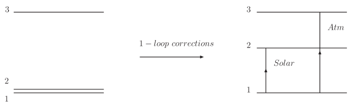
  Figure 1: Neutrino mass scales : tree level dominance

• Loop level dominance : The atmospheric mass² difference originates from one-loop contributions to neutrino masses (Fig. 2).

  

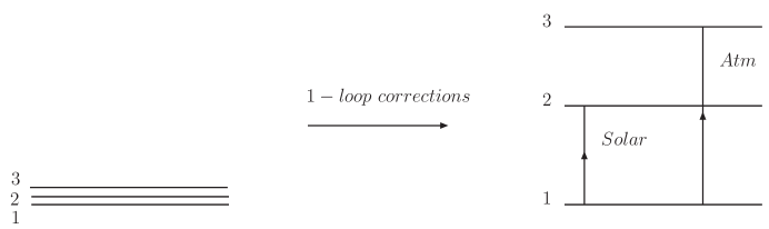
  Figure 2: Neutrino mass scales : loop-level dominance

In either case, the solar mass² difference originates from loop effects from the lepton number violating parameters in (127).

The correct neutrino mass hierarchy can be always generated by the proper choice of just two of the lepton number violating parameters from the list of (127) – one of which sets the scale of the atmospheric mass² difference, the second setting the solar mass² difference. Of course, in the most general case all parameters can contribute.

After choosing the lepton number violating (LNV) parameters, the method described in section 2.4 is then employed to determine the charged lepton Yukawa matrix. In general it needs to be non-diagonal, in order to reproduce correct masses of both neutral and charged leptons and the $U_{MNS}$ mixing matrix. The non-diagonal Yukawa matrix (thus also non-diagonal charged lepton mass matrix), may easily give rise to effects which are already subject to strong experimental bounds; tree level lepton flavour processes, such as $\mu\to e\gamma$ or $\mu\to eee$, are not suppressed and loop corrections to the electron decays will have contributions proportional to the tau mass. To avoid such problems, the specific cases considered in the next sections are those for which the large mixing in the lepton sector, as seen in the MNS matrix, has its origin purely in the neutral sector, and the charged lepton Yukawa couplings remain flavour-diagonal. The formalism we have described thus far allows the correct masses and mixing of charged leptons to be initialised. However, this will lead, in general, to an off-diagonal lepton Yukawa matrix. These, less natural, initial parameters are not necessarily ruled out and within the framework set out above, it is entirely possible to perform the calculations as described. However, we now prefer to consider a set of parameters for which we do not rely on cancellations in the charged lepton sector to make the model phenomenologically viable. The simplest way in which this can be achieved, is to find LNV parameters for which lepton Yukawas are diagonal.

From Eq. (100), for the case where the lepton Yukawa is diagonal and therefore ${\cal Z}_{l}$ is the unit matrix, we see that

$${\cal{Z}}_{\nu}=U_{{MNS}}^{\dagger}\;,$$ (128)

up to higher order terms. Using the MNS matrix as an input, it is possible to see which ratios of entries in the mass matrix give rise to the correct leptonic mixing, being,

$$m_{\nu}^{\textup{\tiny{eff}}}={\cal{Z}}_{\nu}^{*}\>\textup{diag}(m_{1},m_{2},m_{3})\>{\cal{Z}}_{\nu}^{\dagger}=m_{k}\>U_{{MNS}\,ki}\>U_{{MNS}\,kj}\;.$$ (129)

For example, to set the atmospheric scale at tree level, we can see from Eq. (38) that as long as the hierarchy of $\mu_{i}$ matches the ratios of any of the rows in the MNS matrix, the mass matrix follow the correct pattern to be consistent with the observed mixing matrix. If a second mass scale is set up using the pattern dictated by one of the other rows of the MNS matrix, the full MNS matrix will be produced upon diagonalisation.

It is worth noting the nontrivial fact that such an approach, i.e. generating correct structure of neutrino masses and mixings, while keeping FCNC processes in charged lepton sector suppressed, is at all possible.

4.1 Tree level dominance scenario

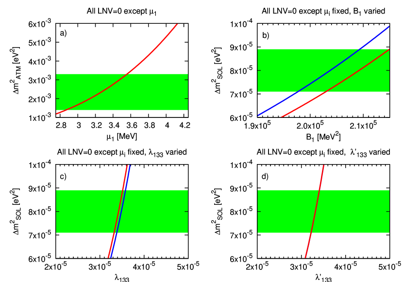
Figure 3: Predictions for atmospheric and solar neutrino mass² differences ($\Delta m^{2}_{\rm ATM}$) and ($\Delta m^{2}_{\rm SOL}$) for the tree level dominance scenario vs. variations of Lepton Number Violating (LNV) parameters as displayed in figure titles. The 3$\sigma$ gray (green) band consistent with experiment is displayed for comparison, as well as the full (gray or red curve) and approximate (dark or blue curve) results. a) Only $\mu_{1}$ is varied. For all other figures, $\mu_{i}$ is fixed as in hierarchy (A) as explained in the text and b) $B_{1}$, or c) $\lambda_{133}$, or d) $\lambda^{\prime}_{133}$, is varied respectively.

At tree level, the mass of a neutrino can be set using $\mu_{i}$ parameters (39). The top left panel in Fig. 3 shows how the value of ($\Delta m^{2}_{\rm ATM}$) varies with $\mu_{1}$ only, setting $\mu_{2,3}=0$. The grey (or red in color) line is the result given by diagonalising the full neutralino matrix in (23) and the dark (blue in color) line is given by (39). They agree perfectly in Fig. 3a and thus only one line is shown. The shaded band shows the current 3$\sigma$ limits. From Eq. (39) it can be seen, however, that it is $|\mu_{1}|^{2}+|\mu_{2}|^{2}+|\mu_{3}|^{2}$ which sets the mass of the tree level neutrino and as such it is straightforward to set any hierarchy between the $\mu_{i}$ and still maintain the same value for the atmospheric difference. To correctly reproduce the MNS matrix, we choose as an input a very simple hierarchy between the $\mu_{i}$ parameters,

$${\rm Hierarchy~{}(A)~{}:}\qquad\mu_{1}=\frac{\mu_{2}}{\sqrt{2}}=\frac{\mu_{3}}{\sqrt{3}}\;.$$ (130)

The scale of all three $\mu_{i}$ is set such that a tree level neutrino of the correct mass is generated which result in the observed atmospheric mass difference, being,

$$\mu_{1}=1.47~{}\textup{MeV}\;,\qquad\mu_{2}=\sqrt{2}\times 1.47~{}\textup{MeV}\;,\qquad\mu_{3}=\sqrt{3}\times 1.47~{}\textup{MeV}\;.$$ (131)

At tree level, this choice of hierarchy gives rise to the MNS matrix, up to the $SU(2)$ rotation described earlier, being driven solely by the neutral sector; the charged lepton mass matrix is diagonal, and as such we have chosen a set of parameters within this basis which avoids the possible phenomenological problems.

A further, single lepton number violating parameter can then be chosen to set the scale of the solar mass² difference. The question of the arbitrariness of the tree level neutrino basis is complicated by the requirement that once the loop corrected mass matrix is diagonalised, ${\cal Z}_{l}$ being the unit matrix is consistent with the experimentally observed MNS matrix. As only one further lepton number violating coupling is initiated, the ratios in which the loop effects are distributed in the loop corrected mass matrix are approximately determined by the tree level mixing matrix. As such we can determine an approximate expression for the extra contribution to the full rotation matrix from rediagonalising the loop effects. The further condition that the full rotation must reproduce the MNS matrix allows us to fix the tree level basis.

The three further Figs. 3(b,c,d) show the range of possible parameters in this scenario. In each of these plots, the set of $\mu_{i}$ are given the values (131) and another, single lepton number violating coupling is varied. In each case, the gray (or red) line shows the full result and the dark (blue) line is the result predicted by the approximate solutions. The fact that $\lambda_{133}$ and $\lambda^{\prime}_{133}$ give the correct solar mass difference over a similar range of parameters is a numerical coincidence. For this example, the factors from the different fermion masses in the quark loop, colour counting and scalar mixing cancel each other.

The contribution of the neutral scalar loop discussed in section 3, results from cancellations between the CP-even and the CP-odd diagrams and may includes contributions of approximately the same order. As such, the approximation presented earlier in the text, Eq. (108), does not agree well with the full result. The discrepancy between the full result and the approximate result reflects the fact that various contributions arise from different places in the full calculation (e.g. the effect on the mixing matrices, the effect on the sneutrino masses). The approximate result plotted in Fig. 3b is given by

$$\Sigma^{D}_{N\,pp} \simeq -\sum_{r=1}^{7}\sum_{i,j=1}^{3}\frac{m_{\kappa^{0}_{r}}{\cal Z}_{\nu\,ip}^{2}}{4(4\pi)^{2}}\left[\frac{e}{c_{W}}{\cal Z}_{N\,1r}-\frac{e}{s_{W}}{\cal Z}_{N\,2r}\right]^{2}\left(\left[\frac{\Delta m_{\tilde{\nu}i}^{2}}{(m_{\tilde{\nu}i}^{2}-m_{\kappa^{0}_{r}}^{2})}-\frac{m_{\kappa^{0}_{r}}^{2}\Delta m_{\tilde{\nu}i}^{2}}{(m_{\tilde{\nu}i}^{2}-m_{\kappa^{0}_{r}}^{2})^{2}}\ln\frac{m_{\kappa^{0}_{r}}^{2}}{m_{\tilde{\nu}i}^{2}}\right]\delta_{ij}\right.$$ (132)

$$+ \left[\frac{B_{i}^{2}\sin^{2}(\beta-\alpha)}{\cos^{2}\beta(M_{H}^{2}-M_{i}^{2})^{2}}+\frac{B_{i}^{2}\cos^{2}(\beta-\alpha)}{\cos^{2}\beta(M_{h}^{2}-M_{i}^{2})^{2}}-\frac{B_{i}^{2}\cos^{2}\beta}{(M_{A}^{2}-M_{i}^{2})^{2}}\right]\delta_{ij}\frac{M_{i}^{2}\ln M_{i}^{2}-m_{\kappa^{0}_{r}}^{2}\ln m_{\kappa^{0}_{r}}^{2}}{M_{i}^{2}-m_{\kappa^{0}_{r}}^{2}}$$

$$+ \left[\frac{B_{i}B_{j}\cos^{2}(\beta-\alpha)}{\cos^{2}\beta(M_{i}^{2}-M_{h}^{2})(M_{j}^{2}-M_{h}^{2})}\right]\frac{M_{h}^{2}\ln M_{h}^{2}-m_{\kappa^{0}_{r}}^{2}\ln m_{\kappa^{0}_{r}}^{2}}{M_{h}^{2}-m_{\kappa^{0}_{r}}^{2}}$$

$$+ \left[\frac{B_{i}B_{j}\sin(\beta-\alpha)}{\cos^{2}\beta(M_{i}^{2}-M_{H}^{2})(M_{j}^{2}-M_{H}^{2})}\right]\frac{M_{H}^{2}\ln M_{H}^{2}-m_{\kappa^{0}_{r}}^{2}\ln m_{\kappa^{0}_{r}}^{2}}{M_{H}^{2}-m_{\kappa^{0}_{r}}^{2}}$$

$$- \left.\left[\frac{B_{i}B_{j}}{\cos^{2}\beta(M_{i}^{2}-M_{A}^{2})(M_{j}^{2}-M_{A}^{2})}\right]\frac{M_{A}^{2}\ln M_{A}^{2}-m_{\kappa^{0}_{r}}^{2}\ln m_{\kappa^{0}_{r}}^{2}}{M_{A}^{2}-m_{\kappa^{0}_{r}}^{2}}\right)\;.$$

The approximate result for the charged scalar loop, given by Eq. (119) agrees well with the full result (Fig. 3c). However, as $\lambda_{133}=-\lambda_{313}$, there are other diagrams which contribute to the full result which are not included in the approximation. The approximate expression captures the important effect. The agreement between the full result and the approximate result, given by Eq. (122) when varying $\lambda^{\prime}_{133}$ (see Fig 3d) is very good, as the diagram highlighted in the text is the only diagram which contributes.

4.2 Loop level dominance scenario

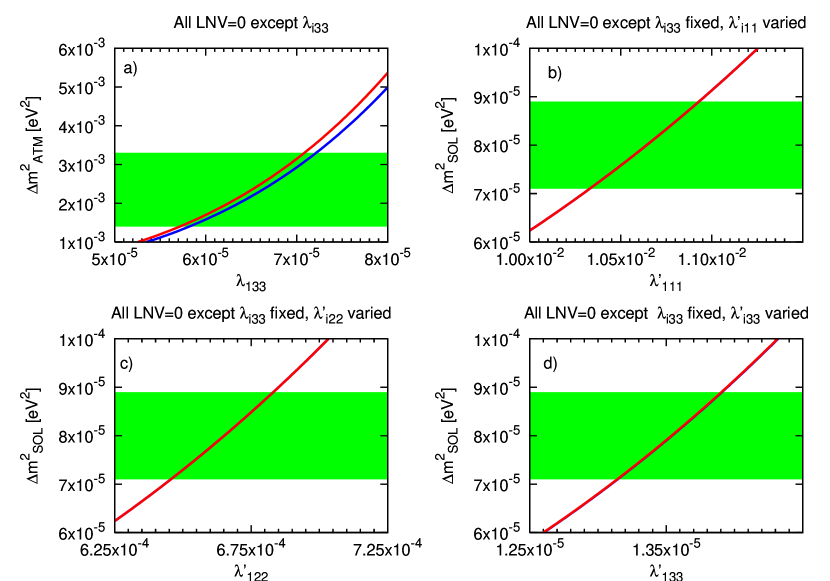
Figure 4: Same as in Fig. 3 but for the loop-level dominance scenario. All LNV parameters are zero apart from a) $\lambda_{i33}$ that is varied in hierarchy (D). For all other figures, $\lambda_{i33}$ is fixed to a value (see the text) consistent with the atmospheric mass² difference and b) only $\lambda^{\prime}_{i11}$ is varied in hierarchy (B) or c) only $\lambda^{\prime}_{i22}$ in hierarchy (B) or d) only $\lambda^{\prime}_{i33}$ in hierarchy (B) in order to accommodate the solar mass² difference.

It is possible for both the solar and the atmospheric scales to be set by loop corrections. This happens if the bilinear parameters $\mu_{i}$ are small enough. In this section we analyse this case setting strictly $\mu_{1}=\mu_{2}=\mu_{3}=0$, so that the one-loop corrections to the full $3\times 3$ neutrino mass matrix are finite. Otherwise a more involved renormalisation scheme has to be implemented.

Again, we would like to set the Lagrangian parameters such that one can generate the correct structure of the MNS matrix while keeping the charged Yukawa couplings flavour-diagonal. This can be achieved if the neutrino mass hierarchy is governed by the trilinear $\lambda$ and $\lambda^{\prime}$ couplings. For the diagrams dominated by trilinear couplings the flavour of the external legs of the loop can be “swapped independently” of the flavour of the particles in the loop, just changing the appropriate indices of the $\lambda,\lambda^{\prime}$ matrices in the loop vertices. Setting the $\lambda$ and $\lambda^{\prime}$ entries which control the couplings of the external legs in certain hierarchies, one can ensure that also the ratios of the various entries in the one loop corrected neutrino mass matrix are such that they give rise to the correct $U_{MNS}$ rotation matrix.

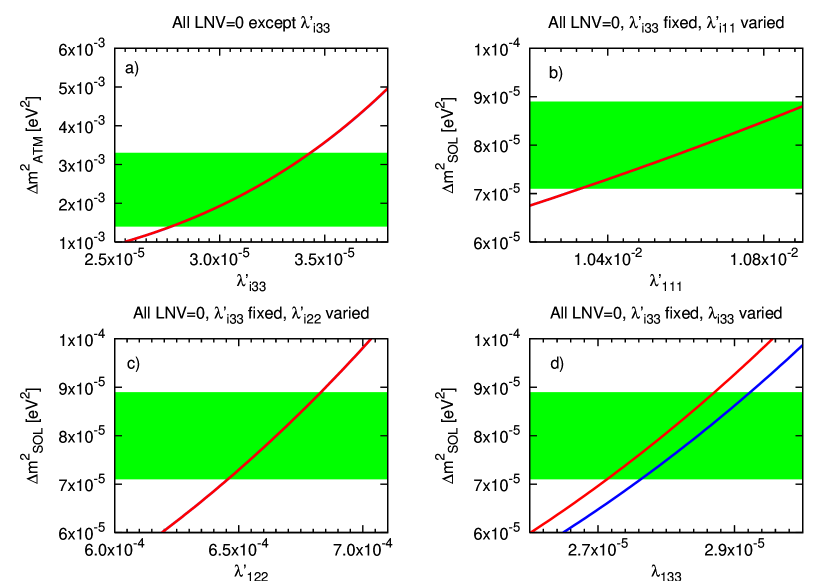
Figure 5: Same as in Fig. 3 but for the loop-level dominance scenario. All LNV parameters are zero apart from a) $\lambda^{\prime}_{i33}$ that is varied in hierarchy (B). For all other figures, $\lambda^{\prime}_{i33}$ is fixed to a value (see the text) consistent with the atmospheric mass² difference and b) only $\lambda^{\prime}_{i11}$ is varied in hierarchy (C) or c) only $\lambda^{\prime}_{i22}$ in hierarchy (C) or d) only $\lambda_{i33}$ in hierarchy (D) in order to accommodate the solar mass² difference.

The possible hierarchies are given by the rows of the MNS matrix and are, with a generic coupling $\lambda^{(^{\prime})}_{ijj}$ as follows,

$${\rm Hierarchy~{}(B)~{}:} \qquad\lambda^{\prime}_{1jj}=\frac{\lambda^{\prime}_{2jj}}{\sqrt{2}}=\frac{\lambda^{\prime}_{3jj}}{\sqrt{3}}$$ (133)

$${\rm Hierarchy~{}(C)~{}:} \qquad\lambda^{\prime}_{1jj}=\frac{\lambda^{\prime}_{2jj}}{\sqrt{2}}=-\frac{\lambda^{\prime}_{3jj}}{\sqrt{3}}$$ (134)

$${\rm Hierarchy~{}(D)~{}:} \qquad\lambda_{1jj}=-\sqrt{2}\lambda_{2jj}\quad\;,\quad\lambda_{3jj}=0\;.$$ (135)

Due to the antisymmetry of the first two indices of $\lambda$ it can only be chosen to follow hierarchy (D) described above.

As the nature of the loop corrections due to $B_{i}$ means that the external legs cannot be swapped without affecting the flavour structure inside the loop, it is difficult to fix a hierarchy of $B_{i}$ in the Lagrangian which will automatically give rise to the correct ratios in the one loop corrected mass matrix.

We consider first, the case where the atmospheric mass² difference is set by $\lambda_{i33}$ in hierarchy (D). The range of values for which the correct atmospheric mass difference is given is plotted in Fig. 4a. Note that although we plot on the x-axis $\lambda_{133}$, the coupling $\lambda_{233}$ is also varying to keep the hierarchy (D) fixed. The fact that both $\lambda_{133}$ and $\lambda_{233}$ contribute is the reason the value of the coupling is only a little greater than the value of $\lambda_{133}$ which correctly reproduces the solar mass difference in the tree-level dominated scenario.

The further three panels [Fig. 4(b-d)] have a fixed set of $\lambda_{i33}$ in hierarchy (D) giving the atmospheric difference. Being,

$$\lambda_{133}=6.7\times 10^{-5}\;,\qquad\lambda_{233}=-\frac{6.7\times 10^{-5}}{\sqrt{2}}\;,\qquad\lambda_{333}=0\;.$$ (136)

$\lambda_{333}=0$ due to the antisymmetry between the first two indices, fitting hierarchy (D). In addition to this, Fig. 4b varies $\lambda^{\prime}_{111,211,311}$ in hierarchy (B) giving the solar mass² difference. Again, we plot the solar mass² difference against the value of $\lambda^{\prime}_{111}$, however $\lambda^{\prime}_{211,311}$ are being varied at the same time. The two remaining panels take in turn different sets of three $\lambda^{\prime}$ couplings, $\lambda^{\prime}_{i22}$ and $\lambda^{\prime}_{i33}$. The final two indices determine which particle is produced in the loop. As such, with a lighter particle in the loop, the couplings must be greater to compensate. We see that, in moving from one panel to the next Fig. 4(b$\to$ d), to produce the same mass difference, a smaller value of the coupling is required with a heavier particle in the loop. With the down quark in the loop (Fig. 4b) the value needed for the coupling may result in large contributions to the neutrinoless double beta decay rate as it is already approaching the excluded regime [53].

Finally, Fig. 5a, we show how the atmospheric mass² difference can be set by the three $\lambda^{\prime}_{i33}$ couplings in hierarchy (B), plotting the result for the atmospheric mass² difference against $\lambda^{\prime}_{133}$. Next, we set $\lambda^{\prime}_{i33}$ to take the following values

$$\lambda^{\prime}_{133}=3.25\times 10^{-5}\;,\qquad\lambda^{\prime}_{233}=\sqrt{2}\times 3.25\times 10^{-5}\;,\qquad\lambda^{\prime}_{333}=\sqrt{3}\times 3.25\times 10^{-5}\;.$$

(137)

The remaining three plots, Fig. 5(b,c,d), show the change in solar mass² difference, as sets of either $\lambda^{\prime}_{i11,i22}$ in hierarchy (C) or the set $\lambda_{i33}$ in hierarchy (D) are varied.

5 Conclusions

An increasingly accurate picture of the neutrino sector, with masses much smaller than the charged leptons and a distinctive mixing matrix in the $W$-vertex, is being discerned by current experiments. We note that there are three preferred ${\cal Z}_{N}$ symmetries in the supersymmetric extension of the Standard Model with minimal particle content. Imposing a ${\cal Z}_{2}$ symmetry results in the widely studied R-parity conserving MSSM, however another preferred symmetry, ${\cal Z}_{3}$, gives rise to a Lagrangian which explicitly violates lepton number. These interactions lead to neutrino masses, both through a ‘see-saw’ type suppression at tree level and through radiative corrections. We have considered the most general scenario in this model; no assumptions have been made concerning CP-violation or intergenerational mixing, for example.

We present, in Appendix A, the tree level mass matrices of the model and, in Appendix B, the full set of Feynman rules for the neutral fermion interactions. The calculation has been performed using two-component Weyl fermion notation; Appendix C contains a derivation of the propagators in this notation, included primarily for pedagogical reason, and generic self-energy diagrams for scalar and gauge boson corrections to fermions.

In the basis set out in our previous work [35], we find that a non-zero neutrino mass will arise at tree level unless all $\mu_{i}$ are zero and analyse in detail, the further contributions to masses that come from loop corrections. We show that the magnitude of the contributions due to neutral fermion loops, examined in section 3.2.1 are determined by the size of the bilinear supersymmetry breaking parameter, $B_{i}$; that loops with charged fermions, described in section 3.2.2, have a contribution due to trilinear lepton number violating couplings in the superpotential, $\lambda_{ijk}$; and that quark loops, section 3.2.3, are determined by the trilinear lepton number violating coupling $\lambda^{\prime}_{ijk}$. Each of these contributions can be dominant. In sections 3.2.4 and 3.2.5, we consider the gauge loops and why they do not give large contributions to neutrinos which are massless at tree level. We derive expressions for the full calculation, which form the basis of our numerical analysis. We also present approximate expressions in each section, which are simple, compact formulas encoding the important information pertaining to each diagram. In our presentation of the results, as seen in Figs. 3,4,5 these simple expressions are shown to be in good agreement with the full result.

The lepton sector in the /L-MSSM is much more involved than the lepton number conserving MSSM. Mixing between leptons, gauginos and higgsinos ensures the question of initialising Lagrangian parameters must be carefully considered. A framework has been constructed in section 2 to correctly reproduce the charged lepton masses and MNS matrix for any set of lepton number violating couplings.

In constructing the framework in which to perform the calculation it is clear that there will be, in general, large intergenerational mixing in the lepton Yukawa matrix, this allows the possibility of unsuppressed tree level flavour violating processes, already subjected to strong bounds. To circumvent this problem we considered sets of Lagrangian parameters for which the MNS matrix has its origin solely in the neutral sector, the lepton Yukawa matrix being diagonal. The three rows of the MNS matrix correspond to three sets of ratios between entries in the loop corrected mass matrix which will give the correct MNS angles. It is possible to set these ratios by setting hierarchies in the couplings between generations. With the condition that it must be possible to change the flavour of the external legs of the diagram without affecting the flavour structure of the loop, there is some freedom in choosing which group of Lagrangian parameters we set in each hierarchy.

Lepton number conserving parameters were fixed to be the SPS1a benchmark point, and we have investigated the effect of varying the lepton number violating couplings, as seen in Figs. 3,4,5. We have shown that values for lepton number violating couplings exist, which give the correct atmospheric and solar mass² difference, charged lepton masses and mixing, which are not already excluded by existing studies of low energy bounds. There are two distinct scenarios that achieve this: the tree level dominance scenario, in which the atmospheric scale is set at tree level and the solar scale set by radiative effects, and another, the loop level dominance scenario, in which both the atmospheric and solar scales are set by radiative corrections.

In the tree level dominance scenario, we choose the $\mu_{i}$ parameters to be of the order of 1 MeV, such that the correct result for the atmospheric mass² difference is obtained. They are chosen to obey a certain hierarchy, which ensures the mixing matrix is consistent with observed MNS.

In addition to this, a further, single lepton number violating coupling can set the scale of the solar mass² difference by determining the contribution of the appropriate loop diagram. It is possible to generate loop diagrams of the appropriate scale, by including either a non-zero $\lambda$,$\lambda^{\prime}$ or $B$ coupling. We find that the correct solar scale can then be set by any of

$$B_{1} \sim 0.21\,\textup{GeV}^{2}\sim\Big{[}\,300\,\mu_{1}\,\Big{]}^{2}\;,$$

$$\lambda_{133} \sim 3.4\times 10^{-5}\sim y_{e}\;,$$

$$\lambda^{\prime}_{133} \sim 3.2\times 10^{-5}\sim 0.1y_{d}\;,$$ (138)

where $y_{e,d}$ is the Yukawa coupling of either the electron or the down quark, presented here merely for the sake of comparison.

In the second case, the correct masses and mixing for both charged and neutral fermions can be achieved without a massive neutrino at tree level. The solar and atmospheric mass² differences both arise from radiative corrections at one loop, using loop contributions whose value is determined by sets of $\lambda$ or $\lambda^{\prime}$ couplings in given hierarchies, such that the observed MNS is generated. Firstly, we show that we can set the atmospheric scale with a set of $\lambda$ couplings of the order of the electron Yukawa coupling, then find the solar scale is correctly set by $\lambda^{\prime}$ couplings of the order of the down quark Yukawa coupling.

Alternatively, the atmospheric scale can be set by $\lambda^{\prime}$ couplings,

$$\lambda^{\prime}_{133}=\frac{\lambda^{\prime}_{233}}{\sqrt{2}}=\frac{\lambda^{\prime}_{333}}{\sqrt{3}}=3.25\times 10^{-5}\sim 0.1y_{d}\;,$$ (139)

and the solar mass² difference can be generated by another set of $\lambda^{\prime}$ couplings,

$$\lambda^{\prime}_{122}=\frac{\lambda^{\prime}_{222}}{\sqrt{2}}=-\frac{\lambda^{\prime}_{322}}{\sqrt{3}}\sim 6.5\times 10^{-4}\sim 2y_{d}\;,$$ (140)

or a set of $\lambda$ couplings of the order of the electron Yukawa.

We include some comments on how this work compares with previous work in the literature. We highlight where our results agree with statements made in the literature and comment on results presented in different bases.

The study of neutrino masses will provide the basis for further work concerning lepton number violating phenomena. The ranges of values for lepton number violating parameters required to produce the correct masses and mixing, will be reflected in processes such as tree level lepton flavour violating decays and will have repercussions concerning rare events such as neutrinoless double beta decay. This will make a valuable link between collider experiments and upcoming neutrino experiments. In this paper, we have made a framework for these investigations.

Appendix A The Lagrangian and the mass matrices of the /L-MSSM 

We strictly follow the notation of Refs. [23, 35]. The /L-MSSM superpotential is given by Eq. (1). The main discussion of this paper is confined in the lepton sector, but for completeness we define here also the mass basis in the quark sector. To this end, we rotate the four quark superfields to a basis where both ${\lambda^{\prime}}^{\phantom{*}}_{\!\!0ij}$ and $\left(Y_{U}\right)^{\phantom{*}}_{ij}$ are diagonal

$$D_{L}^{\prime}\longrightarrow Z^{*}_{d_{L}}D_{L}\;, \bar{D}^{\prime}\longrightarrow Z_{d_{R}}\bar{D}\;,$$

$$U_{L}^{\prime}\longrightarrow Z_{u_{L}}U_{L}\;, \bar{U}^{\prime}\longrightarrow Z^{*}_{u_{R}}\bar{U}\;.$$ (A-1)

By absorbing a rotation matrix into the Lagrangian parameters, one can write down the superpotential (1) as

$$\mathcal{W} = \frac{1}{2}\varepsilon^{\phantom{*}}_{ab}\lambda^{\phantom{*}}_{\alpha\beta j}\mathcal{L}_{\alpha}^{a}\mathcal{L}_{\beta}^{b}\bar{E}_{j}+{\lambda^{\prime}}^{\phantom{*}}_{\!\!\alpha ij}\mathcal{L}_{\alpha}^{1}Q_{i}^{2x}\bar{D}_{j}^{x}-{\lambda^{\prime}}^{\phantom{*}}_{\!\!\alpha kj}K^{*}_{ik}\mathcal{L}_{\alpha}^{2}Q_{i}^{1x}\bar{D}_{j}^{x}-\varepsilon^{\phantom{*}}_{ab}\mu_{\alpha}\mathcal{L}_{\alpha}^{a}{H_{2}}^{b}$$ (A-2)

$$+ \left(Y_{U}\right)^{\phantom{*}}_{ij}Q_{i}^{1x}{H_{2}}^{2}\bar{U}_{j}^{x}-\left(Y_{U}\right)^{\phantom{*}}_{kj}K_{ki}Q_{i}^{2x}{H_{2}}^{1}\bar{U}_{j}^{x}\;,$$

where ${\lambda^{\prime}}^{\phantom{*}}_{\!\!0jk}$ and $\left(Y_{U}\right)^{\phantom{*}}_{ij}$ are diagonal matrices and ${\cal L}^{1}$ (${\cal L}^{2}$) is the neutrino (electron) component of the $SU(2)$ doublet. The charged current part of the Lagrangian,

$${\cal L}_{W}=\frac{e}{\sqrt{2}s_{W}}\bar{u}_{Li}K_{ij}\bar{\sigma}^{\mu}W_{\mu}^{+}d_{Lj}+{\rm H.c}\;,$$ (A-3)

diagrammatically reads (in Weyl spinor notation) as,

(A-5)

with $K_{ij}=Z^{*}_{u_{L}ki}Z^{*}_{d_{L}kj}$ being the CKM matrix. We rotate all fields in the basis where sneutrino vevs are zero. Then the soft supersymmetry breaking terms are,

$$\mathcal{L}_{\rm SSB}=-\left(M^{2}_{\tilde{\rm L}}\right)_{\alpha\beta}\tilde{\nu}^{*}_{L\alpha}\tilde{\nu}^{\phantom{*}}_{L\beta}-\left(M^{2}_{\tilde{\rm L}}\right)_{\alpha\beta}\tilde{e}^{*}_{L\alpha}\tilde{e}^{\phantom{*}}_{L\beta}-m_{{H_{2}}}^{2}h_{2}^{0*}h_{2}^{0}-m_{{H_{2}}}^{2}h_{2}^{+*}h_{2}^{+}$$

$$-\left(m_{\tilde{E}^{c\,}}^{2}\right)_{ij}\tilde{e}^{*}_{Ri}\tilde{e}^{\phantom{*}}_{Rj}-\left(m_{\tilde{Q}}^{2}\right)_{kl}K_{ik}K^{*}_{jl}\tilde{u}^{*z}_{Li}\tilde{u}^{z}_{Lj}-\left(m_{\tilde{Q}}^{2}\right)_{ij}\tilde{d}^{*z}_{Li}\tilde{d}^{z}_{Lj}$$

$$-\left(m_{\tilde{D}^{c}}^{2}\right)_{ij}\tilde{d}^{*z}_{Ri}\tilde{d}^{z}_{Rj}-\left(m_{\tilde{U}^{c}}^{2}\right)_{ij}\tilde{u}^{*z}_{Ri}\tilde{u}^{z}_{Rj}$$

$$\bigg{[}-\left(h_{u}\right)_{ij}\tilde{u}^{y}_{Li}h_{2}^{0}\tilde{u}^{*y}_{Rj}+\left(h_{u}\right)_{kj}K_{ki}\tilde{d}^{y}_{Li}h_{2}^{+}\tilde{u}^{*y}_{Rj}-h_{\alpha\beta k}\tilde{\nu}^{\phantom{*}}_{L\alpha}\tilde{e}^{\phantom{*}}_{L\beta}\tilde{e}^{*}_{Rk}-h^{\prime}_{\alpha jk}\tilde{\nu}^{\phantom{*}}_{L\alpha}\tilde{d}_{Lj}\tilde{d}^{*}_{Rk}\bigg{.}$$

$$+h^{\prime}_{\alpha kj}K^{*}_{ik}\tilde{e}^{\phantom{*}}_{L\alpha}\tilde{u}_{Li}\tilde{d}^{*}_{Rj}+B_{\alpha}\tilde{\nu}^{\phantom{*}}_{L\alpha}h_{2}^{0}-B_{\alpha}\tilde{e}^{\phantom{*}}_{L\alpha}h_{2}^{+}$$

$$\bigg{.}+\frac{1}{2}M_{1}\widetilde{B}\widetilde{B}+M_{2}\widetilde{W}^{+}\widetilde{W}^{-}+\frac{1}{2}M_{2}\widetilde{W}^{0}\widetilde{W}^{0}+\frac{1}{2}M_{3}\widetilde{G}^{R}\widetilde{G}^{R}+\textup{H.c.}\bigg{]}\;,$$ (A-6)

where $B_{\alpha}$ is the four-component bilinear term $B_{\alpha}=(B_{0},B_{i})$ and $h,h^{\prime}$ are trilinear soft breaking couplings. In the basis of [35], in addition to vanishing sneutrino vevs, one obtains also diagonal sneutrino soft breaking mass terms, $\left(M^{2}_{\tilde{\rm L}}\right)_{ij}\equiv\left(\hat{M}^{2}_{\tilde{\rm L}}\right)_{ij}$ is given in Eq. (2.25) of [35]. Notice also that the soft breaking mass which corresponds to the mixing of the Higgs with the slepton is just the term $B_{i}\tan\beta$. In this basis, we shall now present the spectrum of the model. The neutral Higgs sector and approximate formulae has been displayed in Ref. [35]; we repeat only the mass matrices here for completeness and definition.

A.1 Mass Terms for CP-even Neutral Scalars

After electroweak symmetry breaking, sneutrinos, $\{\tilde{\nu}_{L_{i}}\}$, mix with Higgs bosons, $\{\tilde{\nu}_{L0}=h_{1}^{0},h_{2}\}$, resulting in CP-even and CP-odd scalars (recall that CP-symmetry is preserved at tree level even in the most general R-parity violating MSSM [35]). The corresponding CP-even neutral scalar mass terms are

$${\cal L}\ \supset\ -\left(\begin{array}[]{ccc}\mathrm{Re}\,h_{0}^{2}&\mathrm{Re}\,\tilde{\nu}_{L0}&\mathrm{Re}\,\tilde{\nu}_{Li}\end{array}\right)Z^{*}_{R}Z^{T}_{R}\mathcal{M}^{2}_{\rm H}Z_{R}Z^{\dagger}_{R}\left(\begin{array}[]{c}\mathrm{Re}\,h_{0}^{2}\\ \mathrm{Re}\,\tilde{\nu}_{L0}\\ \mathrm{Re}\,\tilde{\nu}_{Lj}\end{array}\right)\;,$$

where

$$\mathcal{M}^{2}_{H}=\left(\begin{array}[]{ccc}{\cos^{2}\beta M_{A}^{2}+\sin^{2}\beta M_{Z}^{2}}&{-\frac{1}{2}\sin 2\beta(M_{A}^{2}+M_{Z}^{2})}&{-B_{j}}\\[8.53581pt] {-\frac{1}{2}\sin 2\beta(M_{A}^{2}+M_{Z}^{2})}&{\sin^{2}\beta M_{A}^{2}+\cos^{2}\beta M_{Z}^{2}}&{B_{j}\tan\beta}\\[8.53581pt] {-B_{i}}&{B_{i}\tan\beta}&{M^{2}_{i}\delta_{ij}}\end{array}\right)\;,$$ (A-10)

and

$$M^{2}_{i}\ \equiv\ (\hat{M}^{2}_{\tilde{\rm L}})_{i}+\frac{1}{2}\cos 2\beta M_{Z}^{2}\;,\qquad M_{A}^{2}=\frac{2B_{0}}{\sin 2\beta}\;.$$ (A-11)

The rotation matrix is then given by

$$Z_{R}^{T}\mathcal{M}^{2}_{\rm H}Z_{R}={\rm diag}[m_{h^{0}}^{2},m_{H^{0}}^{2},(m^{2}_{\tilde{\nu}_{+}})_{i}]\;.\qquad i=1,...3\;.$$ (A-12)

An approximate formula for the matrix $Z_{R}$ is given in Eq. (3.9) of Ref. [35].

A.2 Mass Terms for CP-odd Neutral Scalars

Mass Terms for CP-odd Neutral Scalars can be read from

$${\cal L}\ \supset\ -\left(\begin{array}[]{ccc}\mathrm{Im}\,h_{0}^{2}&\mathrm{Im}\,\tilde{\nu}_{L0}&\mathrm{Im}\,\tilde{\nu}_{Li}\end{array}\right)Z^{*}_{A}Z^{T}_{A}\mathcal{M}^{2}_{\rm A}Z_{A}Z^{\dagger}_{A}\left(\begin{array}[]{c}\mathrm{Im}\,h_{0}^{2}\\ \mathrm{Im}\,\tilde{\nu}_{L0}\\ \mathrm{Im}\,\tilde{\nu}_{Lj}\end{array}\right)\;,$$

where

$$\mathcal{M}^{2}_{\rm A}=\left(\begin{array}[]{ccc}{\cos^{2}\beta M_{A}^{2}+\xi\sin^{2}\beta M_{Z}^{2}}&{\frac{1}{2}\sin 2\beta(M_{A}^{2}-\xi M_{Z}^{2})}&{B_{j}}\\[8.53581pt] {\frac{1}{2}\sin 2\beta(M_{A}^{2}-\xi M_{Z}^{2})}&{\sin^{2}\beta M_{A}^{2}+\xi\cos^{2}\beta M_{Z}^{2}}&{B_{j}\tan\beta}\\[8.53581pt] {B_{i}}&{B_{i}\tan\beta}&{M^{2}_{i}\delta_{ij}}\end{array}\right)\;,$$ (A-16)

and $\xi$ is the gauge-fixing parameter. The rotation matrix $Z_{A}$ is defined through,

$$Z_{A}^{T}\mathcal{M}^{2}_{\rm A}Z_{A}={\rm diag}[m_{G^{0}}^{2},m_{A^{0}}^{2},(m_{\tilde{\nu}_{-}}^{2})_{i}]\;,\qquad i=1,...3\;.$$ (A-17)

An approximate formula for the matrix $Z_{A}$ is given in Eq. (3.22) of Ref. [35].

A.3 Mass Terms for Charged Scalars

In /L-MSSM charged Higgs and charged sleptons mix. The mass terms and the rotation matrix $Z_{H}$, can be read from the Lagrangian

$$\mathcal{L}\supset-\left(\begin{array}[]{cccc}h_{2}^{+*}&h_{1}^{-}&\tilde{e}^{\phantom{*}}_{Lj}&\tilde{e}^{\phantom{*}}_{Rk}\end{array}\right){\cal M}_{H^{+}}^{2}\left(\begin{array}[]{c}h_{2}^{+}\\ h_{1}^{-*}\\ \tilde{e}^{*}_{Li}\\ \tilde{e}^{*}_{Rl}\end{array}\right)=-\left(\begin{array}[]{cccc}h_{2}^{+*}&h_{1}^{-}&\tilde{e}^{\phantom{*}}_{Lj}&\tilde{e}^{\phantom{*}}_{Rk}\end{array}\right)Z_{H}Z^{\dagger}_{H}{\cal M}_{H^{+}}^{2}Z_{H}Z^{\dagger}_{H}\left(\begin{array}[]{c}h_{2}^{+}\\ h_{1}^{-*}\\ \tilde{e}^{*}_{Li}\\ \tilde{e}^{*}_{Rl}\end{array}\right)$$

$$=-(\hat{{\cal M}}^{2}_{H^{+}})_{pq}H^{+*}_{p}H^{+}_{q}\;,\quad p,q=1,...8\;,$$ (A-18)

where the notation is self explanatory and

$${\cal M}_{H^{+}}^{2}=\left(\begin{array}[]{cc|}M_{A}^{2}\cos^{2}\beta+M_{W}^{2}\cos^{2}\beta+\xi M_{W}^{2}\sin^{2}\beta&M_{A}^{2}\sin\beta\cos\beta+M_{W}^{2}(1-\xi)\sin\beta\cos\beta\\ M_{A}^{2}\sin\beta\cos\beta+M_{W}^{2}(1-\xi)\sin\beta\cos\beta&M_{A}^{2}\sin^{2}\beta+\xi M_{W}^{2}\cos^{2}\beta+M_{W}^{2}\sin^{2}\beta\\ B_{j}&B_{j}\tan\beta\\ \frac{1}{\sqrt{2}}\lambda^{*}_{0ml}\mu_{m}v_{d}&\frac{1}{\sqrt{2}}\lambda^{*}_{0ml}\mu_{m}v_{u}\\ \end{array}\right.$$

$$\left.\begin{array}[]{|cc}B_{i}&\frac{1}{\sqrt{2}}\lambda^{\phantom{*}}_{0ml}\mu^{*}_{m}v_{d}\\ B_{i}\tan\beta&\frac{1}{\sqrt{2}}\lambda^{\phantom{*}}_{0ml}\mu^{*}_{m}v_{u}\\ M_{i}^{2}\delta_{ij}-M_{W}^{2}\cos^{2}2\beta\>\delta_{ij}+\frac{1}{2}\lambda^{*}_{0im}\lambda^{\phantom{*}}_{0jm}v_{d}^{2}&\frac{1}{\sqrt{2}}\big{(}-\lambda^{\phantom{*}}_{\alpha jl}\mu^{*}_{\alpha}v_{u}+h_{0jl}v_{d}\big{)}\\ \frac{1}{\sqrt{2}}\big{(}-\lambda^{*}_{\alpha jl}\mu_{\alpha}v_{u}+h^{*}_{0jl}v_{d}\big{)}&\left(m_{\tilde{E}^{c\,}}^{2}\right)_{lk}+(M_{W}^{2}-M_{Z}^{2})\cos^{2}2\beta\>\delta_{lk}+\frac{1}{2}\lambda^{\phantom{*}}_{0ml}\lambda^{*}_{0mk}v_{d}^{2}\\ \end{array}\right)\;.$$ (A-19)

A.4 Mass terms for down-type squarks

Mass terms and rotation matrices for down-type squarks arise from the Lagrangian part

$$-{\cal L}\supset\left(\begin{array}[]{cc}\tilde{d}^{*z}_{Li}&\tilde{d}^{*z}_{Rj}\end{array}\right){\cal{M}}^{2}_{\tiny{\textup{d}}}\left(\begin{array}[]{c}\tilde{d}^{z}_{Lk}\\ \tilde{d}^{z}_{Rl}\end{array}\right) = \left(\begin{array}[]{cc}\tilde{d}^{*z}_{Li}&\tilde{d}^{*z}_{Rj}\end{array}\right)Z^{*}_{\tilde{d}}Z^{T}_{\tilde{d}}{\cal{M}}^{2}_{\tiny{\textup{d}}}Z^{*}_{\tilde{d}}Z^{T}_{\tilde{d}}\left(\begin{array}[]{c}\tilde{d}^{z}_{Lk}\\ \tilde{d}^{z}_{Rl}\end{array}\right)$$ (A-26)

$$= {\hat{\cal{M}}}^{2}_{\tiny{\textup{d}}pq}\>\tilde{d}_{p}^{*z}\tilde{d}_{q}^{z}\;,\qquad p,q=1,...,6$$ (A-27)

where

$${\cal{M}}^{2}_{\tiny{\textup{d}}}=\left(\begin{array}[]{cc}\left(m_{\tilde{Q}}^{2}\right)_{ik}+\frac{1}{2}{\lambda^{\prime}}^{\phantom{*}}_{\!\!0km}{\lambda^{\prime}}^{*}_{\!\!0im}v_{0}^{2}+(\frac{g^{2}}{24}+\frac{g_{2}^{2}}{8})(v_{u}^{2}-v_{0}^{2})\delta_{ik}&-\frac{1}{\sqrt{2}}\mu_{\alpha}{\lambda^{\prime}}^{*}_{\!\!\alpha il}v_{u}+\frac{1}{\sqrt{2}}h^{\prime*}_{0il}v_{0}\\ -\frac{1}{\sqrt{2}}{\lambda^{\prime}}^{\phantom{*}}_{\!\!\alpha kj}\mu^{*}_{\alpha}v_{u}+\frac{1}{\sqrt{2}}h^{\prime}_{0kj}v_{0}&\left(m_{\tilde{D}^{c}}^{2}\right)_{jl}+\frac{1}{2}{\lambda^{\prime}}^{\phantom{*}}_{\!\!0qj}{\lambda^{\prime}}^{*}_{\!\!0ql}v_{0}^{2}+\frac{g^{2}}{12}(v_{u}^{2}-v_{0}^{2})\delta_{jl}\\ \end{array}\right)\;.$$ (A-30)

(A-31)

Recall that ${\lambda^{\prime}}^{\phantom{*}}_{\!\!0km}=\hat{Y}_{{D}k}\,\delta_{km}$ are diagonal down-quark Yukawa couplings.

A.5 Mass terms for up-type squarks

The mass terms for up-type squarks are

$$-{\cal L}=\left(\begin{array}[]{cc}\tilde{u}^{*z}_{Li}&\tilde{u}^{*z}_{Rj}\end{array}\right){\cal{M}}^{2}_{\tiny{\textup{u}}}\left(\begin{array}[]{c}\tilde{u}^{z}_{Lk}\\ \tilde{u}^{z}_{Rl}\end{array}\right) = \left(\begin{array}[]{cc}\tilde{u}^{*z}_{Li}&\tilde{u}^{*z}_{Rj}\end{array}\right)Z_{\tilde{u}}Z^{\dagger}_{\tilde{u}}{\cal{M}}^{2}_{\tiny{\textup{u}}}Z_{\tilde{u}}Z^{\dagger}_{\tilde{u}}\left(\begin{array}[]{c}\tilde{u}^{z}_{Lk}\\ \tilde{u}^{z}_{Rl}\end{array}\right)$$ (A-38)

$$= {\cal{M}}^{2}_{\tiny{\textup{u}}pq}\>\tilde{u}_{p}^{*z}\tilde{u}_{q}^{z}\;,\qquad p,q=1,...,6\;.$$ (A-39)

where

$${\cal{M}}^{2}_{\tiny{\textup{u}}}=$$

$$\left(\begin{array}[]{cc}\left(Km_{\tilde{Q}}^{2}K^{\dagger}\right)_{ik}+\frac{1}{2}(Y_{U}Y_{U}^{\dagger})_{ki}v_{u}^{2}+(\frac{g^{2}}{24}-\frac{g_{2}^{2}}{8})(v_{u}^{2}-v_{0}^{2})\delta_{ik}&\frac{1}{\sqrt{2}}\left(h^{*}_{u}\right)_{jk}v_{u}-\frac{1}{\sqrt{2}}\mu_{0}\left(Y_{U}\right)^{*}_{jk}v_{0}\\ \frac{1}{\sqrt{2}}\left(h_{u}\right)_{li}v_{u}-\frac{1}{\sqrt{2}}\left(Y_{U}\right)^{\phantom{*}}_{li}\mu^{*}_{0}v_{0}&\left(m_{\tilde{U}^{c}}^{2}\right)_{jm}+\frac{1}{2}(Y_{U}Y_{U}^{\dagger})_{jm}v_{u}^{2}-\frac{g^{2}}{6}(v_{u}^{2}-v_{0}^{2})\delta_{jm}\\ \end{array}\right)$$ (A-42)

(A-43)

Recall that $(Y_{U})_{ij}=\hat{Y}_{{U}i}\,\delta_{ij}$ are diagonal up quark Yukawa couplings.

A.6 Mass terms for down quarks

$$\mathcal{L}\supset-\frac{1}{\sqrt{2}}{\lambda^{\prime}}^{\phantom{*}}_{\!\!0ij}v_{d}d^{z}_{Li}d^{z}_{Rj}-\frac{1}{\sqrt{2}}{\lambda^{\prime}}^{*}_{\!\!0ij}v_{d}\bar{d}^{z}_{Li}\bar{d}^{\,z}_{Rj}$$

$$\phantom{\mathcal{L}}=-m_{d\,i}d^{z}_{Li}d^{z}_{Ri}-m_{d\,i}\bar{d}^{z}_{Li}\bar{d}^{\,z}_{Ri}\;,\qquad i=1,...3\;.$$ (A-44)

A.7 Mass terms for up quarks

$$\mathcal{L}\supset-\frac{1}{\sqrt{2}}\left(Y_{U}\right)^{\phantom{*}}_{ij}v_{u}u^{y}_{Rj}u^{y}_{Li}-\frac{1}{\sqrt{2}}\left(Y_{U}\right)^{*}_{ij}v_{u}\bar{u}^{y}_{Rj}\bar{u}^{y}_{Li}$$

$$\phantom{\mathcal{L}}=-m_{u\,i}u^{y}_{Ri}u^{y}_{Li}-m_{u\,i}\bar{u}^{y}_{Ri}\bar{u}^{y}_{Li}\;,\qquad i=1,...3\;.$$ (A-45)

A.8 Mass terms for neutrino-neutralino

$${\cal L}\supset-\frac{1}{2}\left(\begin{array}[]{ccccccc}-i\widetilde{B}&-i\widetilde{W}^{0}&\tilde{h}_{2}^{0}&\nu_{L\alpha}\\ \end{array}\right){\cal{M}}_{\tiny{\textup{N}}}\left(\begin{array}[]{c}-i\widetilde{B}\\ -i\widetilde{W}^{0}\\ \tilde{h}_{2}^{0}\\ \nu_{L\beta}\\ \end{array}\right)-\textup{H.c.}$$

$$\phantom{\mathcal{L}}=-\frac{1}{2}\left(\begin{array}[]{ccccccc}-i\widetilde{B}&-i\widetilde{W}^{0}&\tilde{h}_{2}^{0}&\nu_{L\alpha}\\ \end{array}\right)Z^{*}_{N}Z^{T}_{N}{\cal{M}}_{\tiny{\textup{N}}}Z_{N}Z^{\dagger}_{N}\left(\begin{array}[]{c}-i\widetilde{B}\\ -i\widetilde{W}^{0}\\ \tilde{h}_{2}^{0}\\ \nu_{L\beta}\\ \end{array}\right)+\textup{H.c.}$$

$$\phantom{\mathcal{L}}=-\frac{1}{2}{\hat{\cal{M}}}_{\tiny{\textup{N}}pq}\kappa^{0}_{p}\kappa^{0}_{q}-\frac{1}{2}{\hat{\cal{M}}}^{*}_{\tiny{\textup{N}}pq}\bar{\kappa}^{0}_{p}\bar{\kappa}^{0}_{q}\;,\qquad p,q=1,...7\;.$$ (A-46)

where

$${\cal{M}}_{\tiny{\textup{N}}}=\left(\begin{array}[]{ccccccc}M_{1}&0&\frac{g}{2}v_{u}&-\frac{g}{2}v_{0}\delta_{0\beta}\\ 0&M_{2}&-\frac{g_{2}}{2}v_{u}&\frac{g_{2}}{2}v_{0}\delta_{0\beta}\\ \frac{g}{2}v_{u}&-\frac{g_{2}}{2}v_{u}&0&-\mu_{\beta}\\ -\frac{g}{2}v_{0}\delta_{0\alpha}&\frac{g_{2}}{2}v_{0}\delta_{0\alpha}&-\mu_{\alpha}&0_{\alpha\beta}\\ \end{array}\right)\;.$$ (A-51)

A.9 Mass terms for charged lepton-chargino

$${\cal L}\supset-\left(\begin{array}[]{cc}-i\widetilde{W}^{-}&e_{L\alpha}\end{array}\right){\cal{M}}_{\tiny{\textup{C}}}\left(\begin{array}[]{c}-i\widetilde{W}^{+}\\ \tilde{h}_{2}^{+}\\ e_{Rk}\end{array}\right)\hskip 10.0pt-\hskip 10.0pt\left(\begin{array}[]{cc}i\bar{\widetilde{W}}^{-}&\bar{e}^{\phantom{*}}_{L\alpha}\end{array}\right){\cal{M}}^{*}_{\tiny{\textup{C}}}\left(\begin{array}[]{c}i\bar{\widetilde{W}}^{+}\\ \bar{\tilde{h}}_{2}^{+}\\ \bar{e}^{\phantom{*}}_{Rk}\end{array}\right)$$

$$\phantom{\mathcal{L}}=-\left(\begin{array}[]{cc}-i\widetilde{W}^{-}&e_{L\alpha}\end{array}\right)Z_{-}Z^{\dagger}_{-}{\cal{M}}_{\tiny{\textup{C}}}Z_{+}Z^{\dagger}_{+}\left(\begin{array}[]{c}-i\widetilde{W}^{+}\\ \tilde{h}_{2}^{+}\\ e_{Rk}\end{array}\right)\hskip 10.0pt$$

$$-\hskip 10.0pt\left(\begin{array}[]{cc}i\bar{\widetilde{W}}^{-}&\bar{e}^{\phantom{*}}_{L\alpha}\end{array}\right)Z^{*}_{-}Z^{T}_{-}{\cal{M}}^{*}_{\tiny{\textup{C}}}Z^{*}_{+}Z^{T}_{+}\left(\begin{array}[]{c}i\bar{\widetilde{W}}^{+}\\ \bar{\tilde{h}}_{2}^{+}\\ \bar{e}^{\phantom{*}}_{Rk}\end{array}\right)$$

$$\phantom{\mathcal{L}}=-{\hat{\cal{M}}}_{\tiny{\textup{C}}pq}\kappa^{-}_{p}\kappa^{+}_{q}-{\hat{\cal{M}}}^{*}_{\tiny{\textup{C}}pq}\bar{\kappa}^{-}_{p}\bar{\kappa}^{+}_{q}\;,\qquad p,q=1,...5$$ (A-52)

where

$${\cal{M}}_{\tiny{\textup{C}}}=\left(\begin{array}[]{ccc}M_{2}&\frac{1}{\sqrt{2}}g_{2}v_{u}&0\\ \frac{1}{\sqrt{2}}g_{2}v_{0}\delta_{0\alpha}&\mu_{\alpha}&-\frac{1}{\sqrt{2}}\lambda^{\phantom{*}}_{\alpha 0k}v_{0}\\ \end{array}\right)\;.$$ (A-55)

Appendix B Feynman Rules for Neutral Fermions in the /L-MSSM 

B.1 Neutral Scalar - Neutral Fermion - Neutral Fermion interactions

$\displaystyle-\frac{ie}{2c_{W}}Z_{R1q}Z_{N3p}Z_{N1r}+\frac{ie}{2s_{W}}Z_{R1q}Z_{N2p}Z_{N3r}$ $\displaystyle+\frac{ie}{2c_{W}}Z_{R(2+\alpha)q}Z_{N(4+\alpha)p}Z_{N1r}-\frac{ie}{2s_{W}}Z_{R(2+\alpha)q}Z_{N2p}Z_{N(4+\alpha)r}$ $\displaystyle-\frac{ie}{2c_{W}}Z_{R1q}Z_{N3r}Z_{N1p}+\frac{ie}{2s_{W}}Z_{R1q}Z_{N2r}Z_{N3p}$ $\displaystyle+\frac{ie}{2c_{W}}Z_{R(2+\alpha)q}Z_{N(4+\alpha)r}Z_{N1p}-\frac{ie}{2s_{W}}Z_{R(2+\alpha)q}Z_{N2r}Z_{N(4+\alpha)p}$

$\displaystyle-\frac{e}{2c_{W}}Z_{A1q}Z_{N3p}Z_{N1r}+\frac{e}{2s_{W}}Z_{A1q}Z_{N2p}Z_{N3r}$ $\displaystyle+\frac{e}{2c_{W}}Z_{A(2+\alpha)q}Z_{N(4+\alpha)p}Z_{N1r}-\frac{e}{2s_{W}}Z_{A(2+\alpha)q}Z_{N2p}Z_{N(4+\alpha)r}$ $\displaystyle-\frac{e}{2c_{W}}Z_{A1q}Z_{N3r}Z_{N1p}+\frac{e}{2s_{W}}Z_{A1q}Z_{N2r}Z_{N3p}$ $\displaystyle+\frac{e}{2c_{W}}Z_{A(2+\alpha)q}Z_{N(4+\alpha)r}Z_{N1p}-\frac{e}{2s_{W}}Z_{A(2+\alpha)q}Z_{N2r}Z_{N(4+\alpha)p}$

B.2 Charged Scalar - Neutral Fermion - Charged Fermion interactions

$\displaystyle-i\frac{e}{s_{W}}Z_{H(2+\alpha)q}Z^{*}_{-1p}Z_{N(4+\alpha)r}$ $\displaystyle-i\lambda^{\phantom{*}}_{\alpha\beta j}Z_{H(5+j)q}Z^{*}_{-(2+\beta)p}Z_{N(4+\alpha)r}$ $\displaystyle+i\frac{e}{\sqrt{2}c_{W}}Z_{H(2+\alpha)q}Z^{*}_{-(2+\alpha)p}Z_{N1r}$ $\displaystyle+i\frac{e}{\sqrt{2}s_{W}}Z_{H(2+\alpha)q}Z_{N2r}Z^{*}_{-(2+\alpha)p}$

$\displaystyle-i\lambda^{\phantom{*}}_{\alpha\beta j}Z^{*}_{H(2+\beta)q}Z_{+(2+j)p}Z_{N(4+\alpha)r}$ $\displaystyle-i\sqrt{2}\frac{e}{c_{W}}Z^{*}_{H(5+i)q}Z_{+(2+i)p}Z_{N1r}$ $\displaystyle-i\frac{e}{\sqrt{2}c_{W}}Z^{*}_{H1q}Z_{+2p}Z_{N1r}-i\frac{e}{s_{W}}Z^{*}_{H1q}Z_{+1p}Z_{N3r}$ $\displaystyle-i\frac{e}{\sqrt{2}s_{W}}Z^{*}_{H1q}Z_{N2r}Z_{+2p}$

B.3 Squark - Neutral Fermion - Quark interactions

$\displaystyle-i{\lambda^{\prime}}^{\phantom{*}}_{\!\!\alpha jk}Z_{\tilde{d}(3+k)q}Z_{N(4+\alpha)p}-i\frac{e}{3\sqrt{2}c_{W}}Z_{\tilde{d}jq}Z_{N1p}$ $\displaystyle+i\frac{e}{\sqrt{2}s_{W}}Z_{\tilde{d}jq}Z_{N2p}$

$\displaystyle-i{\lambda^{\prime}}^{\phantom{*}}_{\!\!\alpha ij}Z^{*}_{\tilde{d}iq}Z_{N(4+\alpha)p}-i\frac{e\sqrt{2}}{3c_{W}}Z^{*}_{\tilde{d}(3+j)q}Z_{N1p}$

$\displaystyle-i\frac{e}{3\sqrt{2}c_{W}}Z^{*}_{\tilde{u}jq}Z_{N1p}-i\left(Y_{U}\right)^{\phantom{*}}_{jk}Z^{*}_{\tilde{u}(3+k)q}Z_{N3p}$ $\displaystyle-i\frac{e}{\sqrt{2}s_{W}}Z^{*}_{\tilde{u}jq}Z_{N2p}$

$\displaystyle i\frac{2e\sqrt{2}}{3c_{W}}Z_{\tilde{u}(3+k)q}Z_{N1p}-i\left(Y_{U}\right)^{\phantom{*}}_{ik}Z_{\tilde{u}iq}Z_{N3p}$

B.4 Fermion - Fermion - Gauge boson interactions

$\displaystyle\frac{ie}{2s_{W}c_{W}}\bigg{[}Z^{*}_{N(4+\alpha)r}Z_{N(4+\alpha)q}-Z^{*}_{N3r}Z_{N3q}\bigg{]}\bar{\sigma}^{\mu}$

$\displaystyle i\bigg{[}\frac{e}{\sqrt{2}s_{W}}Z^{*}_{N(4+\alpha)r}Z^{*}_{-(2+\alpha)q}+\frac{e}{s_{W}}Z^{*}_{N2r}Z^{*}_{-1q}\bigg{]}\bar{\sigma}^{\mu}$

$\displaystyle i\bigg{[}\frac{e}{\sqrt{2}s_{W}}Z^{*}_{N3r}Z_{+2q}-\frac{e}{s_{W}}Z^{*}_{N2r}Z_{+1q}\bigg{]}\bar{\sigma}^{\mu}$

Appendix C Weyl spinors and self-energy one-loop corrections

Throughout this article we make an extensive use of Weyl spinor notation. Generally speaking, working with Weyl spinors is advantageous because of two reasons : first they appear naturally in a supersymmetric Lagrangian (no extra work is required to make the connection with Dirac or Majorana four-component spinors and their corresponding Feynman rules) and second, when used in Feynman diagrams, they present transparently their structure as for example, the dominance of a particle mass or the appearance of a mixing etc. In this Appendix we give a pedagogical introduction to the use of Weyl fermion propagators and vertices. We then calculate at the end the generic self energies that appear in (LABEL:con1, LABEL:con2). This Appendix is complementary to the work of Ref. [45].

Using path integral technics we want to find the propagator of a massive Weyl fermion in Minkowski space. The path integral involving a Weyl fermion $\xi^{\alpha}(x)$ and a source field $J^{\alpha}(x)$ is

$$W[J,\bar{J}]\ =\ N\int d[\xi]\>d[\bar{\xi}]\>e^{iS[\xi,\bar{\xi},J,\bar{J}]}\;,$$ (C-1)

where $N$ is a constant and

$$i\>S[\xi,\bar{\xi},J,\bar{J}]\ =\ i\>\int d^{4}x\biggl{\{}\frac{1}{2}\biggl{[}i\bar{\xi}\bar{\sigma}^{\mu}\partial_{\mu}\xi+i\xi\sigma^{\mu}\partial_{\mu}\bar{\xi}-m(\xi\xi+\bar{\xi}\bar{\xi})\biggr{]}+J\xi+\bar{J}\bar{\xi}\biggr{\}}\;.$$ (C-2)

In writing the above action functional we use the conventions of Wess and Bagger [48] with the metric being $g_{\mu\nu}=(1,-1,-1,-1)$. It is simpler to work in momentum space and thus we Fourier transform (in four dimensions) both fields and sources as

$$\xi^{\alpha}(x)\ = \ \int_{-\infty}^{+\infty}\frac{d^{4}p}{(2\pi)^{2}}\>e^{ip\cdot x}\>\xi^{\alpha}(p)\;,\qquad\bar{\xi}^{\dot{\alpha}}(x)\ =\ \int_{-\infty}^{+\infty}\frac{d^{4}p}{(2\pi)^{2}}\>e^{-ip\cdot x}\>\bar{\xi}^{\dot{\alpha}}(p)\;,$$

$$J^{\alpha}(x)\ = \ \int_{-\infty}^{+\infty}\frac{d^{4}p}{(2\pi)^{2}}\>e^{ip\cdot x}\>J^{\alpha}(p)\;,\qquad\bar{J}^{\dot{\alpha}}(x)\ =\ \int_{-\infty}^{+\infty}\frac{d^{4}p}{(2\pi)^{2}}\>e^{-ip\cdot x}\>\bar{J}^{\dot{\alpha}}(p)\;,$$ (C-3)

where $p\cdot x\equiv p_{\mu}x^{\mu}$. We also make use of the four dimensional definition of the $\delta$-function,

$$\delta(x-x^{\prime})\ =\ \int_{-\infty}^{+\infty}\frac{d^{4}p}{(2\pi)^{4}}\>e^{ip\cdot(x-x^{\prime})}\>.$$ (C-4)

The action functional (C-2) is conveniently written in a matrix notation

$$i\>\int d^{4}p\>\frac{1}{2}\biggl{(}\Omega^{\dagger}{\cal M}\Omega+\Omega^{\dagger}X+X^{\dagger}\Omega\biggr{)}\;,$$ (C-5)

where

$$\Omega(p)\equiv\left(\begin{array}[]{c}\xi_{\alpha}(-p)\\[8.53581pt] \bar{\xi}^{\dot{\alpha}}(p)\end{array}\right)\;,\quad X(p)\equiv\left(\begin{array}[]{c}\bar{J}^{\dot{\alpha}}(p)\\[8.53581pt] J_{\alpha}(-p)\end{array}\right)\;,\quad{\cal M}(p)\equiv\left(\begin{array}[]{cc}\bar{\sigma}\cdot p&-m\\[8.53581pt] -m&\sigma\cdot p\end{array}\right)\;,$$ (C-12)

where $\sigma\cdot p=\sigma^{\mu}_{\alpha\dot{\beta}}\>p_{\mu}$ and $\bar{\sigma}\cdot p=\bar{\sigma}_{\mu}^{\dot{\alpha}\beta}\>p^{\mu}$ and the matrix ${\cal M}$ is hermitian. The path integral measure does not change when transforming the Weyl fermions $\xi$ by a constant $(J)$ as

$$\Omega\ =\ \Omega^{\prime}-{\cal M}^{-1}\>X\;.$$ (C-13)

After this transformation is applied in (C-5), sources and fields “get decoupled”

$$i\>\int d^{4}p\>\frac{1}{2}\left(\Omega^{{}^{\prime}\dagger}{\cal M}\Omega^{\prime}-X^{\dagger}{\cal M}^{-1}X\right)\;,$$ (C-14)

where the inverse of M is easily found to be

$${\cal M}^{-1}\ =\ \frac{1}{p^{2}-m^{2}}\>\left(\begin{array}[]{cc}\sigma\cdot p&m\\[8.53581pt] m&\bar{\sigma}\cdot p\end{array}\right)\;.$$ (C-17)

The first integrand term in (C-14) is exactly the same as the one in square brackets of (C-2). Recalling that $X=X[J,\bar{J}]$ the path integral in (C-1) takes the form

$$W[J,\bar{J}]\ =\ Ne^{iS_{0}[\xi,\bar{\xi}]}\>\exp\left\{-\frac{i}{2}\int d^{4}p\>X^{\dagger}{\cal M}^{-1}X\right\}=W[0]\>\exp\left\{-\frac{i}{2}\int d^{4}p\>X^{\dagger}{\cal M}^{-1}X\right\}\;,$$

where $S_{0}$ is the free Weyl fermion action functional

$$S_{0}[\xi,\bar{\xi}]\ =\ \int d^{4}x\left[i\bar{\xi}\bar{\sigma}^{\mu}\partial_{\mu}\xi-\frac{1}{2}m(\xi\xi+\bar{\xi}\bar{\xi})\right]\;.$$ (C-19)

The propagators for the Weyl fermions can be read from

$$\exp\left\{-\frac{i}{2}\int d^{4}p\>X^{\dagger}{\cal M}^{-1}X\right\} = -\frac{1}{2}\int d^{4}p\left\{J^{\beta}(p)\frac{i\sigma_{\beta\dot{\alpha}}\cdot p}{p^{2}-m^{2}}\bar{J}^{\dot{\alpha}}(p)+\bar{J}_{\dot{\alpha}}(p)\left[\frac{-i\bar{\sigma}^{\dot{\alpha}\beta}\cdot p}{p^{2}-m^{2}}\right]J_{\beta}(p)\right.$$ (C-20)

$$+ \left.J^{\alpha}(p)\frac{im\delta_{\alpha}^{\beta}}{p^{2}-m^{2}}J_{\beta}(-p)+\bar{J}_{\dot{\alpha}}(-p)\frac{im\delta^{\dot{\alpha}}_{\dot{\beta}}}{p^{2}-m^{2}}\bar{J}^{\dot{\beta}}(p)\right\}\;.$$

Diagrammatically the propagator of a massive Weyl fermion is depicted in Fig. 6.

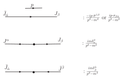
Figure 6: Massive Weyl spinor propagators.

The convention we adopt here is that arrows run away from dotted indices at a vertex and towards undotted indices at a vertex. As it is obvious from (C-20), the kinetic part of the propagator [the top one in Fig. 6] is uniquely defined from the height of the indices that link this propagator with the vertex.

The propagator for two different Weyl spinors $\eta$ and $\psi$ (forming a Dirac spinor in four component notation) with action functional,

$$i\>S[\xi,\bar{\xi},J,\bar{J}] = i\>\int d^{4}x\biggl{\{}\biggl{[}i\>\bar{\eta}\bar{\sigma}^{\mu}\partial_{\mu}\eta+i\>\bar{\psi}\bar{\sigma}^{\mu}\partial_{\mu}\psi-m(\eta\psi+\bar{\eta}\bar{\psi})\biggr{]}+J_{\eta}\eta+J_{\bar{\eta}}\bar{\eta}+J_{\psi}\psi+J_{\bar{\psi}}\bar{\psi}\biggr{\}}$$

$$\;.$$ (C-21)

have the same form as in (C-20) with obvious Lorentz invariant substitutions. Vertices with Weyl fermions arise from the superpotential and from the supersymmetric gauge interactions. They are displayed in Fig. 7.

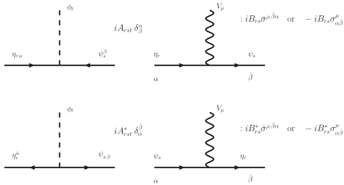
Figure 7: General vertices involving Weyl spinors used in this article. In case of the vector boson vertex the Feynman rule is defined completely from the height that link a propagator with this vertex. Vertices on the left arise from ${\cal L}_{Y}=A_{rst}\phi_{t}\psi_{s}\eta_{r}+A_{rst}^{*}\phi_{t}^{*}\bar{\psi}_{s}\bar{\eta}_{r}$ and vertices on the right arise from ${\cal L}=B_{rs}\bar{\psi}_{s}\bar{\sigma}^{\mu}V_{\mu}\eta_{r}+B^{*}_{rs}\bar{\eta}_{r}\bar{\sigma}^{\mu}V_{\mu}^{*}\psi_{s}$.

We now proceed in calculating the general self energies of (LABEL:con1,LABEL:con2). The 1PI self energy, $\Sigma^{D}$, obtains corrections from diagrams which have either gauge particles or scalar particles in the loop. The scalar contributions for general scalar-fermion vertices $iA_{qrs}$ and $iB_{prs}$ is

where $m_{\psi\eta_{r}}$ denotes the physical mass of the mass eigenstate which is composed out of the interaction eigenstates $\psi_{r}$ and $\eta_{r}$. The corresponding neutrino self energy arising from vector boson contributions with generic vertices $iC_{qr}\bar{\sigma}^{\mu}$ and $iD_{qr}\bar{\sigma}^{\mu}$ is

$$\Sigma^{D}_{pq}(m^{2}_{\kappa^{0}_{q}}) = iD_{pr}C_{qr}m_{\psi\eta_{r}}\frac{i\pi^{2}}{(2\pi)^{4}\mu^{4-D}}\Bigg{\{}(\xi+3)B_{0}(m^{2}_{\kappa^{0}_{q}},m^{2}_{V},m^{2}_{\psi\eta_{r}})+$$ (C-23)

$$+ (\xi-1)\xi m^{2}_{V}C_{0}(0,m^{2}_{\kappa^{0}_{q}},m^{2}_{\kappa^{0}_{q}},m^{2}_{V},\xi m^{2}_{V},m^{2}_{\psi\eta_{r}})\Bigg{\}}\;,$$

where $\xi$ is the gauge fixing parameter, $m_{V}$ is the mass of the vector boson and $B_{0},C_{0}$ are the Passarino-Veltman functions [46] in the notation of Ref. [47],

$$B_{0}(q^{2},m_{\phi}^{2},m_{\psi}^{2}) = \frac{(2\pi)^{4}\mu^{4-D}}{i\pi^{2}}\int\frac{d^{D}k}{(2\pi)^{D}}\frac{1}{(k^{2}-m_{\phi}^{2})\>([q+k]^{2}-m_{\psi}^{2})}\;,$$ (C-24)

$$C_{0}(0,q^{2},q^{2},m_{V}^{2},\xi m_{V}^{2},m_{\psi}^{2}) = \frac{(2\pi)^{4}\mu^{4-D}}{i\pi^{2}}\int\frac{d^{D}k}{(2\pi)^{D}}\frac{1}{(k^{2}-m_{V}^{2})\>(k^{2}-\xi m_{V}^{2})\>([q+k]^{2}-m_{\psi}^{2})}\;.$$

Finally, self energy corrections to the Weyl fermion kinetic terms read as

and

where $B_{1},C_{2}$ are defined in [47].

References

• [1] P. Fayet, “Spontaneously Broken Supersymmetric Theories Of Weak, Electromagnetic And Strong Interactions,” Phys. Lett. B 69, 489 (1977); G. R. Farrar and P. Fayet, “Phenomenology Of The Production, Decay, And Detection Of New Hadronic States Associated With Supersymmetry,” Phys. Lett. B 76 (1978) 575; S. Weinberg, “Supersymmetry At Ordinary Energies. 1. Masses And Conservation Laws,” Phys. Rev. D 26, 287 (1982). For a reviews see, H. K. Dreiner, “An introduction to explicit R-parity violation,” arXiv:hep-ph/9707435; G. Bhattacharyya, “R-parity-violating supersymmetric Yukawa couplings: A mini-review,” Nucl. Phys. Proc. Suppl.  52A (1997) 83 [arXiv:hep-ph/9608415]; M. Chemtob, “Phenomenological constraints on broken R parity symmetry in supersymmetry models,” Prog. Part. Nucl. Phys.  54 (2005) 71 [arXiv:hep-ph/0406029].
• [2] L. E. Ibanez and G. G. Ross, “Discrete gauge symmetries and the origin of baryon and lepton number conservation in supersymmetric versions of the standard model,” Nucl. Phys. B 368, 3 (1992).
• [3] H. K. Dreiner, C. Luhn and M. Thormeier, “What is the discrete gauge symmetry of the MSSM?,” arXiv:hep-ph/0512163.
• [4] S. Eidelman et al. [Particle Data Group], “Review of particle physics,” Phys. Lett. B 592 (2004) 1.
• [5] L. J. Hall and M. Suzuki, “Explicit R Parity Breaking In Supersymmetric Models,” Nucl. Phys. B 231 (1984) 419.
• [6] A. S. Joshipura and M. Nowakowski, “’Just so’ oscillations in supersymmetric standard model,” Phys. Rev. D 51 (1995) 2421 [arXiv:hep-ph/9408224].
• [7] T. Banks, Y. Grossman, E. Nardi and Y. Nir, “Supersymmetry without R-parity and without lepton number,” Phys. Rev. D 52 (1995) 5319 [arXiv:hep-ph/9505248].
• [8] M. Nowakowski and A. Pilaftsis, “W and Z boson interactions in supersymmetric models with explicit R-parity violation,” Nucl. Phys. B 461 (1996) 19 [arXiv:hep-ph/9508271].
• [9] H. P. Nilles and N. Polonsky, “Supersymmetric neutrino masses, R-symmetries, and the generalized mu problem,” Nucl. Phys. B 484 (1997) 33 [arXiv:hep-ph/9606388].
• [10] A. H. Chamseddine and H. K. Dreiner, “A new mechanism to solve the small scale problem of local supersymmetry,” Phys. Lett. B 389 (1996) 533 [arXiv:hep-ph/9607261].
• [11] R. Hempfling, “Neutrino Masses and Mixing Angles in SUSY-GUT Theories with explicit R-Parity Breaking,” Nucl. Phys. B 478 (1996) 3 [arXiv:hep-ph/9511288].
• [12] D. E. Kaplan and A. E. Nelson, “Solar and atmospheric neutrino oscillations from bilinear R-parity violation,” JHEP 0001 (2000) 033 [arXiv:hep-ph/9901254].
• [13] M. Hirsch, M. A. Diaz, W. Porod, J. C. Romao and J. W. F. Valle, “Neutrino masses and mixings from supersymmetry with bilinear R-parity violation: A theory for solar and atmospheric neutrino oscillations,” Phys. Rev. D 62 (2000) 113008 [Erratum-ibid. D 65 (2002) 119901] [arXiv:hep-ph/0004115].
• [14] M. A. Diaz, M. Hirsch, W. Porod, J. C. Romao and J. W. F. Valle, “Solar neutrino masses and mixing from bilinear R-parity broken supersymmetry: Analytical versus numerical results,” Phys. Rev. D 68 (2003) 013009 [Erratum-ibid. D 71 (2005) 059904] [arXiv:hep-ph/0302021].
• [15] A. Abada, S. Davidson and M. Losada, “Neutrino masses and mixings in the MSSM with soft bilinear R(p) violation,” Phys. Rev. D 65 (2002) 075010 [arXiv:hep-ph/0111332].
• [16] M. Hirsch, H. V. Klapdor-Kleingrothaus and S. G. Kovalenko, Phys. Lett. B 398, 311 (1997) [arXiv:hep-ph/9701253].
• [17] Y. Grossman and H. E. Haber, “Sneutrino mixing phenomena,” Phys. Rev. Lett.  78 (1997) 3438 [arXiv:hep-ph/9702421].
• [18] Y. Grossman and H. E. Haber, Phys. Rev. D 59 (1999) 093008 [arXiv:hep-ph/9810536].
• [19] Y. Grossman and S. Rakshit, “Neutrino masses in R-parity violating supersymmetric models,” Phys. Rev. D 69 (2004) 093002 [arXiv:hep-ph/0311310].
• [20] S. Davidson and M. Losada, “Neutrino masses in the R(p) violating MSSM,” JHEP 0005 (2000) 021 [arXiv:hep-ph/0005080].
• [21] B. de Carlos and P. L. White, “R-parity Violation Effects through Soft Supersymmetry Breaking Terms and the Renormalisation Group,” Phys. Rev. D 54 (1996) 3427 [arXiv:hep-ph/9602381].
• [22] E. Nardi, “Renormalization group induced neutrino masses in supersymmetry without R-parity,” Phys. Rev. D 55 (1997) 5772 [arXiv:hep-ph/9610540].
• [23] B. C. Allanach, A. Dedes and H. K. Dreiner, “The R parity violating minimal supergravity model,” Phys. Rev. D 69 (2004) 115002 [arXiv:hep-ph/0309196].
• [24] F. M. Borzumati, Y. Grossman, E. Nardi and Y. Nir, “Neutrino masses and mixing in supersymmetric models without R parity,” Phys. Lett. B 384 (1996) 123 [arXiv:hep-ph/9606251].
• [25] F. Borzumati and J. S. Lee, Phys. Rev. D 66, 115012 (2002) [arXiv:hep-ph/0207184].
• [26] M. Drees, S. Pakvasa, X. Tata and T. ter Veldhuis, “A supersymmetric resolution of solar and atmospheric neutrino puzzles,” Phys. Rev. D 57 (1998) 5335 [arXiv:hep-ph/9712392].
• [27] E. J. Chun, S. K. Kang, C. W. Kim and U. W. Lee, “Supersymmetric neutrino masses and mixing with R-parity violation,” Nucl. Phys. B 544 (1999) 89 [arXiv:hep-ph/9807327].
• [28] A. S. Joshipura and S. K. Vempati, “Sneutrino vacuum expectation values and neutrino anomalies through trilinear R-parity violation,” Phys. Rev. D 60 (1999) 111303 [arXiv:hep-ph/9903435].
• [29] K. Choi, K. Hwang and E. J. Chun, “Atmospheric and solar neutrino masses from horizontal U(1) symmetry,” Phys. Rev. D 60, 031301 (1999) [arXiv:hep-ph/9811363].
• [30] O. C. W. Kong, “Neutrino oscillations and flavor structure of supersymmetry without R-parity,” Mod. Phys. Lett. A 14 (1999) 903 [arXiv:hep-ph/9808304].
• [31] S. Rakshit, G. Bhattacharyya and A. Raychaudhuri, Phys. Rev. D 59 (1999) 091701 [arXiv:hep-ph/9811500].
• [32] R. Adhikari and G. Omanovic, “LSND, solar and atmospheric neutrino oscillation experiments, and R-parity violating supersymmetry,” Phys. Rev. D 59 (1999) 073003.
• [33] A. Abada, G. Bhattacharyya and M. Losada, “A general analysis with trilinear and bilinear R-parity violating couplings in the light of recent SNO data,” Phys. Rev. D 66 (2002) 071701 [arXiv:hep-ph/0208009]; A. Abada and M. Losada, “Constraints on both bilinear and trilinear R-parity violating couplings from neutrino laboratories and astrophysics data,” Phys. Lett. B 492 (2000) 310 [arXiv:hep-ph/0007041].
• [34] S. Rakshit, Mod. Phys. Lett. A 19 (2004) 2239 [arXiv:hep-ph/0406168].
• [35] A. Dedes, S. Rimmer, J. Rosiek and M. Schmidt-Sommerfeld, “On the neutral scalar sector of the general R-parity violating MSSM,” Phys. Lett. B 627 (2005) 161 [arXiv:hep-ph/0506209].
• [36] H. K. Dreiner and M. Thormeier, “Supersymmetric Froggatt-Nielsen models with baryon- and lepton-number violation,” Phys. Rev. D 69 (2004) 053002 [arXiv:hep-ph/0305270].
• [37] M. Bisset, O. C. W. Kong, C. Macesanu and L. H. Orr, “A simple phenomenological parametrization of supersymmetry without R-parity,” Phys. Lett. B 430, 274 (1998) [arXiv:hep-ph/9804282].
• [38] See for instance, R. A.  Horn and C. R.  Johnson, Topics in Matrix analysis, Cambridge University Press, 1991; Carl D. Meyer, Matrix Analysis and Applied Linear Algebra, Siam, 2000.
• [39] Z. Maki, M. Nakagawa and S. Sakata, “Remarks On The Unified Model Of Elementary Particles,” Prog. Theor. Phys.  28 (1962) 870; B. Pontecorvo, “Neutrino Experiments And The Question Of Leptonic-Charge Conservation,” Sov. Phys. JETP 26 (1968) 984 [Zh. Eksp. Teor. Fiz.  53 (1967) 1717].
• [40] J. Schechter and J. W. F. Valle, “Neutrino Decay And Spontaneous Violation Of Lepton Number,” Phys. Rev. D 25 (1982) 774.
• [41] M. Gell-Mann, M. P. Ramond and R. Slansky, 1979, in Supergravity, edited by P. van Nieuwenhuizen and D.Z. Freedman (North Holland); T Yanagida, in Proceedings of Workshop on Unified Theory and Baryon Number in the Universe, edited by O. Sawada and A. Sugamoto (KEK); R. N. Mohapatra and G. Senjanovic, “Neutrino Mass And Spontaneous Parity Nonconservation,” Phys. Rev. Lett.  44 (1980) 912.
• [42] S. Y. Choi, J. Kalinowski, G. Moortgat-Pick and P. M. Zerwas, “Analysis of the neutralino system in supersymmetric theories,” Eur. Phys. J. C 22, 563 (2001) [Addendum-ibid. C 23, 769 (2002)] [arXiv:hep-ph/0108117].
• [43] M. Misiak, S. Pokorski and J. Rosiek, Adv. Ser. Direct. High Energy Phys.  15 (1998) 795 [arXiv:hep-ph/9703442].
• [44] B. A. Kniehl and A. Pilaftsis, “Mixing Renormalization in Majorana Neutrino Theories,” Nucl. Phys. B 474, 286 (1996) [arXiv:hep-ph/9601390]; A. Pilaftsis, “Gauge and scheme dependence of mixing matrix renormalization,” Phys. Rev. D 65, 115013 (2002) [arXiv:hep-ph/0203210].
• [45] H. Haber, “Practical Methods for treating Majorana fermions”, lecture given at Pre-SUSY 2005, http://www.ippp.dur.ac.uk/pre-SUSY05/ . See also, H.K. Dreiner, H. E. Haber and S. P. Martin, unpublished.
• [46] G. Passarino and M. J. G. Veltman, “One Loop Corrections For E+ E- Annihilation Into Mu+ Mu- In The Weinberg Model,” Nucl. Phys. B 160 (1979) 151;
• [47] T. Hahn and M. Perez-Victoria, “Automatized one-loop calculations in four and D dimensions,” Comput. Phys. Commun.  118, 153 (1999) [arXiv:hep-ph/9807565]. See also “LoopTools user guide” in http://www.feynarts.de/looptools/.
• [48] J. Wess and J. Bagger, “Supersymmetry and supergravity,” Princeton Series in Physics.
• [49] T. Schwetz, “Neutrino oscillations: Current status and prospects,” Acta Phys. Polon. B 36 (2005) 3203 [arXiv:hep-ph/0510331].
• [50] P. F. Harrison, D. H. Perkins and W. G. Scott, “Tri-bimaximal mixing and the neutrino oscillation data,” Phys. Lett. B 530 (2002) 167 [arXiv:hep-ph/0202074].
• [51] B. C. Allanach et al., “The Snowmass points and slopes: Benchmarks for SUSY searches,” in Proc. of the APS/DPF/DPB Summer Study on the Future of Particle Physics (Snowmass 2001) ed. N. Graf, Eur. Phys. J. C 25, 113 (2002) [eConf C010630, P125 (2001)] [arXiv:hep-ph/0202233].
• [52] B. C. Allanach, “SOFTSUSY: A C++ program for calculating supersymmetric spectra,” Comput. Phys. Commun.  143, 305 (2002) [arXiv:hep-ph/0104145].
• [53] B. C. Allanach, A. Dedes and H. K. Dreiner, “Bounds on R-parity violating couplings at the weak scale and at the GUT scale,” Phys. Rev. D 60 (1999) 075014 [arXiv:hep-ph/9906209].