Unitary coupled channel analysis of the $\Lambda(1520)$ resonance

Abstract

We study the $\Lambda(1520)$ resonance in a coupled channel approach involving the $\pi\Sigma(1385)$, $K\Xi(1530)$, $\bar{K}N$ and $\pi\Sigma$ channels. Implementing unitarity in coupled channels, we make an analysis of the relative importance of the different mechanisms which contribute to the dynamical structure of this resonance. From experimental information on some partial wave amplitudes and constraints imposed by unitarity, we get a comprehensive description of the amplitudes and hence the couplings to the different channels. We test these amplitudes in different reactions like $K^{-}p\to\Lambda\pi\pi$, $\gamma p\to K^{+}K^{-}p$, $\gamma p\to K^{+}\pi^{0}\pi^{0}\Lambda$ and $\pi^{-}p\to K^{0}K^{-}p$ and find a fair agreement with the experimental data.

1 Introduction

The ${\Lambda(1520)}$ ($3/2^{-}$, $D_{03}$) resonance is capturing renewed attention, particularly since it appears invariably in searches of pentaquarks in photononuclear reactions [1, 2] in $\gamma p\to K^{+}K^{-}p$ and $\gamma d\to\ K^{+}K^{-}np$. Since getting signals for pentaquarks involves cuts in the spectrum and subtraction of backgrounds, the understanding of the resonance properties and the strength of different reactions in the neighborhood of the peak becomes important in view of a correct interpretation of invariant mass spectra when cuts and background subtractions are made.

There is another reason that justifies a thorough study of the ${\Lambda(1520)}$ resonance. Indeed, much progress has been done interpreting the low lying $1/2^{-}$ resonances as dynamically generated from the interaction of the octet of pseudoscalar mesons with the octet of stable baryons [3, 4, 5, 6, 7] which allows one to make predictions for resonance formation in different reactions [8]. One of the surprises on this issue was the realization that the $\Lambda(1405)$ resonance is actually a superposition of two states, a wide one coupling mostly to $\pi\Sigma$ and a narrow one coupling mostly to $\bar{K}N$ [5, 9, 10]. The performance of a recent experiment on the $K^{-}p\to\pi^{0}\pi^{0}\Sigma^{0}$ reaction [11] and comparison with older ones, particularly the $\pi^{-}p\to K^{0}\pi\Sigma$ reaction [12], has brought evidence on the existence of these two $\Lambda(1405)$ states [13]. Extension of these works to the interaction of the octet of pseudoscalar mesons with the decuplet of baryons has led to the conclusion that the low lying $3/2^{-}$ baryons are mostly dynamically generated objects [14, 15]. One of these states is the ${\Lambda(1520)}$ resonance which is generated from the interaction of the coupled channels $\pi\Sigma(1385)$ and $K\Xi(1530)$, and couples mostly to the first channel to the point that, in this picture, the state would qualify as a quasibound $\pi\Sigma^{*}$ state. Indeed, the nominal mass of the ${\Lambda(1520)}$ is a few MeV below the average of the $\pi\Sigma^{*}$ mass. However, the PDG [16] gives a width of $15\textrm{ MeV}$ for the ${\Lambda(1520)}$, with branching ratios of $45$% into $\bar{K}N$ and $43$% into $\pi\Sigma$, and only a small branching ratio of the order of $4$% for $\pi\Sigma^{*}$ which could be of the order of $10$% according to some analysis [17] which claims that about $85$% of the decay into $\pi\pi\Lambda$ is actually $\pi\Sigma^{*}$. The association of $\pi\pi\Lambda$ to $\pi\Sigma^{*}$ in the peak of the ${\Lambda(1520)}$ is a non trivial test since one has no phase space for $\pi\Sigma^{*}$ excitation and only the width of the $\Sigma^{*}$ allows for this decay, hence precluding the reconstruction of the $\Sigma^{*}$ resonant shape from the $\pi\Lambda$ decay product. Our theoretical study here will allow a more precise determination from the study of $K^{-}p\to\pi^{0}\pi^{0}\Lambda$ reaction [18], which proceeds mostly via $K^{-}p\to\pi^{0}(\Sigma^{*0})\to\pi^{0}(\pi^{0}\Lambda)$ and involves the $\Sigma^{*}$ propagator, overcoming the reconstruction of the $\Sigma^{*}$ through the $\pi\Lambda$ invariant mass. In any case, the large branching ratios to $\bar{K}N$ and $\pi\Sigma$, of the order of $90$% together, indicate that the $\bar{K}N$ and $\pi\Sigma$ channels must play a relevant role in building up the resonance.

In the present work we tackle this problem by performing a coupled channel analysis of the ${\Lambda(1520)}$ data with $\pi\Sigma^{*}$, $K\Xi^{*}$, $\bar{K}N$ and $\pi\Sigma$, the first two channels interacting in $s$-wave and the last two channels in $d$-wave to match the $3/2^{-}$ spin and parity of the ${\Lambda(1520)}$ resonance.

Anticipating results we shall see that although the $\pi\Sigma^{*}$ remains with the largest coupling to ${\Lambda(1520)}$, its strength is reduced with respect to the simpler picture of only $\pi\Sigma^{*}$ building up the resonance, and at the same time there is a substantial coupling to $\bar{K}N$ and $\pi\Sigma$ which distorts the original $\pi\Sigma^{*}$ quasibound picture and makes the $\bar{K}N$ and $\pi\Sigma$ channels relevant in the interpretation of different reactions.

The procedure followed in this paper is the following: first we carry out a fit to $\bar{K}N\to\bar{K}N$ and $\bar{K}N\to\pi\Sigma$ data in $d$-waves for $I=0$ in order to determine a few unknown parameters beyond the transition potentials of the $\pi\Sigma^{*}$, $K\Xi^{*}$, subsystems which are provided by chiral Lagrangians [15, 14]. With this input we make predictions for the $K^{-}p\to\pi^{0}\pi^{0}\Lambda$ and $K^{-}p\to\pi^{+}\pi^{-}\Lambda$ reactions, providing absolute cross sections in good agreement with experiment. Furthermore, we also make predictions for the shape of the $K^{-}p$ mass distribution for the $\gamma p\to K^{+}K^{-}p$ and $\pi^{-}p\to K^{+}K^{-}p$ reactions and for the absolute value of the ratio of the $\gamma p\to K^{+}\pi^{0}\pi^{0}\Lambda$ and $\gamma p\to K^{+}K^{-}p$ reactions at the peak of the ${\Lambda(1520)}$ resonance, for which there are no experimental data available.

The work provides a good model for the ${\Lambda(1520)}$ resonance within a unitary coupled channel approach, which goes beyond the simpler picture of the resonance as a quasibound $\pi\Sigma^{*}$ state, and provides a framework to study other reactions involving the production of the ${\Lambda(1520)}$.

2 Formalism

In Ref.[19] the $\Lambda(1520)$ resonance was studied within a coupled channel formalism including the $\pi\Sigma^{*}$, $K\Xi^{*}$ in $s$-wave and the $\bar{K}N$ and $\pi\Sigma$ in $d$-waves leading to a good reproduction of the pole position of the $\Lambda(1520)$ of the scattering amplitudes. However, the use of the pole position to get the properties of the resonance is far from being accurate as soon as a threshold is opened close to the pole position on the real axis, which is the present case with the $\pi\Sigma^{*}$ channel. Apart from that, in the approach of Ref. [19] some matrix elements in the kernel of the Bethe-Salpeter (BS) equation were not considered. In the present work we aim at a more precise description of the physical processes involving the $\Lambda(1520)$ resonance. Hence, we introduce the rest of tree level transition potentials relevant for the analysis: $\bar{K}N\to\bar{K}N$, $\bar{K}N\to\pi\Sigma$ and $\pi\Sigma\to\pi\Sigma$. Analogously to Ref. [19], we use for these vertices effective transition potentials which are proportional to the incoming and outgoing momentum squared in order to account for the $d$-wave character of the channels. Denoting $\pi\Sigma^{*}$, $K\Xi^{*}$, $\bar{K}N$ and $\pi\Sigma$ channels by $1$, $2$, $3$ and $4$ respectively, the matrix containing the tree level amplitudes is written as:

$$V=\left|\begin{array}[]{cccc}C_{11}(k_{1}^{0}+k_{1}^{0})&C_{12}(k_{1}^{0}+k_{2}^{0})&\gamma_{13}\,q_{3}^{2}&\gamma_{14}\,q^{2}_{4}\\ C_{21}(k_{2}^{0}+k_{1}^{0})&C_{22}(k_{2}^{0}+k_{2}^{0})&0&0\\ \gamma_{13}\,q_{3}^{2}&0&\gamma_{33}\,q^{4}_{3}&\gamma_{34}\,q_{3}^{2}\,q^{2}_{4}\\ \gamma_{14}\,q^{2}_{4}&0&\gamma_{34}\,q_{3}^{2}\,q_{4}^{2}&\gamma_{44}\,q^{4}_{4}\end{array}\right|~{},$$ (1)

where $q_{i}=\frac{1}{2\sqrt{s}}\sqrt{[s-(M_{i}+m_{i})^{2}][s-(M_{i}-m_{i})^{2}]}$, $k_{i}^{0}=\frac{s-M_{i}^{2}+m_{i}^{2}}{2\sqrt{s}}$ and $M_{i}(m_{i})$ is the baryon(meson) mass. The coefficients $C_{ij}$ are $C_{11}=\frac{-1}{f^{2}}$, $C_{21}=C_{12}=\frac{\sqrt{6}}{4f^{2}}$ and $C_{22}=\frac{-3}{4f^{2}}$, where $f$ is $1.15f_{\pi}$, with $f_{\pi}$ ($=93\textrm{ MeV}$) the pion decay constant, which is an average between $f_{\pi}$ and $f_{K}$ as was used in Ref. [4] in the related problem of the dynamical generation of the $\Lambda(1405)$.

The elements $V_{11}$, $V_{12}$, $V_{21}$, $V_{22}$ come from the lowest order chiral Lagrangian involving the decuplet of baryons and the octet of pseudoscalar mesons as discussed in Ref. [15, 14]. We neglect the elements $V_{23}$ and $V_{24}$ which involve the tree level interaction of the $K\Xi^{*}$ channel to the $d$-wave channels because the $K\Xi^{*}$ threshold is far away from the ${\Lambda(1520)}$ and its role in the resonance structure is far smaller than that of the $\pi\Sigma^{*}$.

In the literature several unitarization procedures have been used to obtain a scattering matrix fulfilling unitarity in coupled channels, like the Inverse Amplitude Method [20, 21] or the $N/D$ method [22]. In this latter work the equivalence with the Bethe-Salpeter equation used in [23] was established.

In the present work we use the Bethe-Salpeter equation with the $V$ given above as the kernel to obtain the unitarized amplitude $T$:

$$T=V+VGT\Rightarrow T=[1-VG]^{-1}V$$ (2)

Diagrammatically this means that one is resumming the series expressed in Fig. 1.

Figure 1: Diagrammatic representation of the resummation of meson-baryon loops in the unitarization procedure.

Following [19], the relationship of the scattering matrix $T$ used in the unitary framework to the actual $t$ matrix in the Mandl-Shaw normalization [24] is given by

$$t_{\pi\Sigma^{*}\rightarrow\pi\Sigma^{*}} = T_{\pi\Sigma^{*}\rightarrow\pi\Sigma^{*}}\,,$$

$$t_{K\Xi^{*}\rightarrow K\Xi^{*}} = T_{K\Xi^{*}\rightarrow K\Xi^{*}}\,,$$

$$t_{\bar{K}N\rightarrow\pi\Sigma^{*}} = T_{\bar{K}N\rightarrow\pi\Sigma^{*}}\ {\cal C}(\tfrac{1}{2}\ 2\ \tfrac{3}{2};m,M-m)Y_{2,m-M}(\hat{k})(-1)^{M-m}\sqrt{4\pi}\,,$$

$$t_{\pi\Sigma\rightarrow\pi\Sigma^{*}} = T_{\pi\Sigma\rightarrow\pi\Sigma^{*}}\ {\cal C}(\tfrac{1}{2}\ 2\ \tfrac{3}{2};m,M-m)Y_{2,m-M}(\hat{k})(-1)^{M-m}\sqrt{4\pi}\,,$$

$$t_{\bar{K}N\rightarrow\bar{K}N} = T_{\bar{K}N\rightarrow\bar{K}N}\ \sum_{M}{\cal C}(\tfrac{1}{2}\ 2\ \tfrac{3}{2};m,M-m)Y_{2,m-M}(\hat{k})\,\times$$ (3)

$$\times {\cal C}(\tfrac{1}{2}\ 2\ \tfrac{3}{2};m^{\,\prime},M-m^{\,\prime})Y_{2,m^{\,\prime}-M}^{*}(\hat{k}^{\,\prime})(-1)^{m^{\,\prime}-m}\ 4\pi\,.$$

The amplitudes $t_{\bar{K}N\to\pi\Sigma}$ and $t_{\pi\Sigma\to\pi\Sigma}$ have the same form as $t_{\bar{K}N\to\bar{K}N}$ but changing $T_{\bar{K}N\to\bar{K}N}$ by $T_{\bar{K}N\to\pi\Sigma}$ and $T_{\pi\Sigma\to\pi\Sigma}$ respectively.

In Eq. (2) $G$ stands for a diagonal matrix containing the loop functions involving a baryon and a meson [5] and is given by:

$$G_{l}(\sqrt{s},M_{l},m_{l}) = i\,2M_{l}\int\frac{d^{4}q}{(2\pi)^{4}}\,\frac{1}{(P-q)^{2}-M_{l}^{2}+i\epsilon}\,\frac{1}{q^{2}-m^{2}_{l}+i\epsilon}$$ (4)

$$= \frac{2M_{l}}{16\pi^{2}}\left\{a_{l}(\mu)+\ln\frac{M_{l}^{2}}{\mu^{2}}+\frac{m_{l}^{2}-M_{l}^{2}+s}{2s}\ln\frac{m_{l}^{2}}{M_{l}^{2}}-2i\pi\frac{q_{l}}{\sqrt{s}}\right.$$

$$\!\!\!\!\!\!\!\!\!\!\phantom{\frac{2M}{16\pi^{2}}}+\frac{q_{l}}{\sqrt{s}}\left[\ln(s-(M_{l}^{2}-m_{l}^{2})+2q_{l}\sqrt{s})+\ln(s+(M_{l}^{2}-m_{l}^{2})+2q_{l}\sqrt{s})\right.$$

$$\!\!\!\!\!\!\!\!\!\!\left.\phantom{\frac{2M}{16\pi^{2}}+\frac{q_{l}}{\sqrt{s}}}\left.-\ln(s-(M_{l}^{2}-m_{l}^{2})-2q_{l}\sqrt{s})-\ln(s+(M_{l}^{2}-m_{l}^{2})-2q_{l}\sqrt{s})\right]\right\}\,,$$

where $\mu$ is the scale of dimensional regularization, $s=P^{2}$ with $P$ the total four-momentum of the meson-baryon system and $a_{l}$ are unknown subtraction constants. For the loops related to the $s$-wave channels ($\pi\Sigma^{*}$ and $K\Xi^{*}$) it has a natural size of around $-2$, as has been obtained in many different works [5, 25, 26]. For the $d$-wave channels ($\bar{K}N$ and $\pi\Sigma$) there is no such estimate in the literature. We expect it to be larger compared to the $s$-wave subtraction constant since it is likely to contain part of the off-shell contribution of the potentials in the loop, which are expected to be large for the $d$-wave vertices. In Eq. (2) the momentum dependence of the tree level amplitudes has been factorized out of the loop integral. For the $s$-wave vertices this has been justified e.g. in [23, 4]. For the $d$-wave vertices we assume that the off-shell momentum dependences can be reabsorbed in the couplings and the subtraction constants which are free parameters in our scheme. We will discuss further on this issue below.

Since the $\pi\Sigma^{*}$ threshold lies in the $\Lambda(1520)$ region the consideration of the width of the $\Sigma^{*}$ resonance in the loop function is crucial in order to account properly for this channel. The $\Sigma^{*}$ width is about $35\textrm{ MeV}$ while the $\Lambda(1520)$ width is only about $15\textrm{ MeV}$. Since the threshold effects are very important in the description involving coupled channels (due e.g. to the opening of sources of imaginary parts), this implies that the proper consideration of the spectral distribution of the $\Sigma^{*}$ resonance is essential. This is achieved through the convolution of the $\pi\Sigma^{*}$ loop function with the spectral distribution considering the $\Sigma^{*}$ width:

$${G}_{\pi\Sigma^{*}}(\sqrt{s},M_{\Sigma^{*}},m_{\pi})\to\int_{M_{\Sigma^{*}}-2\Gamma_{0}}^{M_{\Sigma^{*}}+2\Gamma_{0}}d\sqrt{s^{\prime}}\ \frac{-1}{\pi}\,\textrm{Im}\left[\frac{1}{\sqrt{s^{\prime}}-M_{\Sigma^{*}}+i\Gamma_{\Sigma^{*}}(s^{\prime})/2}\right]G_{\pi\Sigma^{*}}(\sqrt{s},\sqrt{s^{\prime}},m_{\pi})$$ (5)

where

$$\Gamma_{\Sigma^{*}}(s^{\prime})=\Gamma_{0} \left(0.88\frac{q^{3}(s^{\prime},M_{\Lambda}^{2},m_{\pi}^{2})}{q^{3}(M_{\Sigma}^{*2},M_{\Lambda}^{2},m_{\pi}^{2})}\Theta(\sqrt{s^{\prime}}-M_{\Lambda}-m_{\pi})\right.$$ (6)

$$+ \left.\quad 0.12\frac{q^{3}(s^{\prime},M_{\Sigma}^{2},m_{\pi}^{2})}{q^{3}(M_{\Sigma}^{*2},M_{\Sigma}^{2},m_{\pi}^{2})}\Theta(\sqrt{s^{\prime}}-M_{\Sigma}-m_{\pi})\right),$$

with $\Gamma_{0}$ being the on-shell $\Sigma^{*}$ total decay width. In Eq. (6) we have assumed a $p$-wave decay of the $\Sigma^{*}$ into $\Lambda\pi$ ($88$%) and $\Sigma\pi$ ($12$%). This consideration of the $\Sigma^{*}$ width is also an improvement from the previous work of Ref. [19].

Note that we could think of other states in our coupled channels of the vector-meson–baryon (VB) type like $K^{*}N$, $\rho\Sigma$, etc. In fact, as we discuss in detail after Eq. (18), the $K^{*}N\Lambda(1520)$ coupling can be large in some models [27, 28]. The explicit consideration of these channels in the coupled channel formalism is unnecessary for the following reasons: the thresholds for the VB states quoted above are $1830\textrm{ MeV}$ and $1967\textrm{ MeV}$, more than $300\textrm{ MeV}$ above the energy of the $\Lambda(1520)$. As a consequence, their contribution to the scattering amplitudes around the $\Lambda(1520)$ region is very weakly energy dependent, since the corresponding VB loop functions are weakly energy dependent far away from the VB threshold. Thus, their contribution can be easily incorporated in terms of the subtraction constants introduced in Eq. (4) which are fitted to data. This appears to be also the case in the study of the $\pi N$ interaction in [29], where, for instance, $\rho$ exchange in the t-channel (in tensor form) is used to generate higher order terms in the framework, but not as $\rho N$ or $\rho\Delta$  s-channel intermediate states. Note that, even if the contribution of these new channels was not numerically negligible, this would not mean that such channels are important in the structure of the resonance, since what matters for the wave function components are the derivatives of the resonance selfenergy from these channels with respect to the energy [30].

As explained before, in Eq. (1) the $C_{ij}$ coefficients are obtained from the lowest order chiral Lagrangians accounting for the Weinberg-Tomozawa term. One could include in the kernel of the BS equation contributions of the higher order Lagrangians of the pseudoscalar octet and baryon decuplet interaction in the $SU(3)$ sector, but this has not been thoroughly studied. Some work is however done in the $SU(2)$ sector [31]. The situation is different in the interaction of the pseudoscalar octet with the baryon octet, where work has been done including higher order Lagrangians [32, 33] in the strange sector. However, it is worth stressing that already a good reproduction of the data is obtained with the lowest order chiral Lagrangian [32, 33, 4, 5]. The effect of higher order Lagrangians can be accounted for to some extent by means of the subtraction constants of the loop functions (or equivalently fixing a cutoff to data [4]). In the present work we have more subtraction constants, as well as unknown $\gamma$ parameters, which are fitted to the data, so there is plenty of room to effectively account for the effect of higher order Lagrangians by means of all these free parameters.

In the SU(2) sector there is more work. Interesting developments are done in Ref.  [34] dealing with pions and nucleons, where higher order Lagrangians are introduced, together with the $\Delta(1232)$ as an explicit degree of freedom, in such a way as to respect decoupling. Decoupling [35] states that in the chiral limit the leading non analytic corrections (LNAC) to S-matrix elements and related magnitudes are given solely in terms of the meson and baryon degrees of freedom, U and B terms of the Lagrangian, and that the inclusion of mesonic ($\rho,\omega$) or baryonic ($\Delta,N^{*})$ resonances in the pertinent loops does not modify the LNACs. Another interesting development is done in [29] where the higher order terms are obtained by using explicitly the exchange of resonances. The framework respects unitarity in coupled channels and matches at low energies with the perturbative results of [36], thus providing an example of the resonance saturation hypothesis [37] in the baryon sector. Developments along these lines in the meson-octet baryon-decuplet interaction would be certainly welcome.

3 Results

In the model described so far we have as unknown parameters $\gamma_{13}$, $\gamma_{14}$, $\gamma_{33}$, $\gamma_{34}$, $\gamma_{44}$ in the $V$ matrix. Apart from these, there is also the freedom in the value of the subtraction constants in the loop functions. We will consider one subtraction constant for the $s$-wave channels ($a_{0}$) and one for the $d$-wave ones ($a_{2}$). Despite the apparent large number of free parameters in the $V$ matrix, it is worth emphasizing that the largest matrix elements are $V_{11}$, $V_{12}$ and $V_{22}$ [15] which come from a chiral Lagrangian [38] without any free parameters. Due to the $d$-wave behavior the other ones are expected to be smaller, as we will see below.

In order to obtain these parameters we fit our model to the experimental results on the $\bar{K}N$ and $\pi\Sigma$ scattering amplitudes in $d$-wave and $I=0$. We use experimental data from Refs. [39, 40] where $\bar{K}N\to\bar{K}N$ and $\bar{K}N\to\pi\Sigma$ amplitudes are provided from partial wave analysis. These experimental amplitudes are related to the amplitudes of Eq. (2) through

$$\tilde{T}_{ij}(\sqrt{s})=-\sqrt{\frac{M_{i}q_{i}}{4\pi\sqrt{s}}}\sqrt{\frac{M_{j}q_{j}}{4\pi\sqrt{s}}}\,T_{ij}(\sqrt{s})$$ (7)

where $M$ and $q$ are the baryon mass and the on-shell C.M. momentum of the specific channel.

It is also interesting to make connection with another standard notation for the amplitudes for the scattering of spin $0$ with spin $1/2$ particles:

$$M = f+ig\,\vec{\sigma}\cdot\hat{n}$$

$$f = \frac{1}{q}\sum_{l=0}^{\infty}\left[(l+1)f_{l+}+lf_{l-}\right]P_{l}(\cos\theta)$$

$$g = \frac{1}{q}\sum_{l=1}^{\infty}\left[f_{l+}-f_{l-}\right]P^{\prime}_{l}(\cos\theta)\sin\theta,$$ (8)

where $\hat{n}=(\vec{q}_{i}\times\vec{q}_{j})/|\vec{q}_{i}\times\vec{q}_{j}|$. For $l=2$, $J=3/2$, only $f_{l-}$ contributes and we find, given the normalizations introduced in Eq. (3),

$$f_{l-}=\tilde{T}_{ii}$$ (9)

and similarly for the amplitudes $\tilde{T}_{ij}$ where $i$, $j$ stand for the $\bar{K}N$ and $\pi\Sigma$ channels. The elastic cross section is given by $\sigma=4\pi l|f_{l-}|^{2}/q^{2}$ $(l=2)$.

We now write the amplitude $T_{ij}$ close to a resonance peak as

$$T_{ij}=\frac{g_{i}g_{j}}{\sqrt{s}-M_{R}+i\Gamma/2},$$ (10)

(note that, for $l=2$, the $q_{i}^{2}$ factor is incorporated in $g_{i}$). We then have

$$\Gamma_{i}=\frac{g_{i}^{2}}{2\pi}\frac{M_{i}}{M_{R}}q_{i}=-\frac{1}{2\pi}\frac{\Gamma}{2}ImT_{ii}\frac{M_{i}}{M_{R}}q_{i}$$ (11)

and hence

$$B_{i}=\frac{\Gamma_{i}}{\Gamma}=Im\tilde{T}_{ii}(\sqrt{s}=M_{R}).$$ (12)

Note that due to the appearance of the $q_{i}$, $q_{j}$ factors, Eq. (7) can only be applied for channels which are open. For those which are close to threshold the decay can only proceed via the overlap of the mass distributions of the resulting products including their width, with the mass of the decaying resonance, and this situation requires another treatment, as we shall see below.

In Fig. 2 we show the result of our fit to the experimental data.

Figure 2: Fit to the experimental amplitudes. Left column: $\bar{K}N\to\bar{K}N$; right column: $\bar{K}N\to\pi\Sigma$.

The first column represents the real and imaginary parts (top and bottom respectively) of the $\tilde{T}_{33}$ and the last column denotes the same for $\tilde{T}_{34}$ along with the experimental data of [39, 40]. In order to restrict the freedom in the parameters of the model we have also introduced data for the $\pi\Sigma\to\pi\Sigma$ amplitude. The data are not given in [39, 40]. However, the results given in that paper for the $\bar{K}N\to\bar{K}N$ and $\bar{K}N\to\pi\Sigma$ are results of analysis of raw data. The same analysis would have provided

$$T_{\pi\Sigma\to\pi\Sigma}=\frac{(T_{\bar{K}N\to\pi\Sigma})^{2}}{T_{\bar{K}N\to\bar{K}N}}$$ (13)

given the resonant structure of the amplitudes. By introducing these data we are forcing the resulting model to fulfill this property, which helps constrain the freedom in the fit parameters. In the data from [39, 40] which we have considered, no errors are given. In order to perform a fit to the data some errors need to be assigned. We have taken a reasonable criteria by assigning an error of $0.03$ to each point except the ones close to the peak where an error of $0.01$ is taken to enforce the resonance character of the data. We have checked that other reasonable assumptions also lead to about the same solutions. It is worth noting that the shape of the amplitudes is rather asymmetric, in the sense that it differs from a Breit-Wigner shape. This is a consequence of the $d$-wave behavior and also of the non trivial internal dynamics imposed by unitarity in coupled channels.

The values of the unknown parameters obtained from the fit are given in Table 1.

$a_{0}$	$a_{2}$	$\gamma_{13}$ $(\textrm{MeV}^{-3})$	$\gamma_{14}$ $(\textrm{MeV}^{-3})$	$\gamma_{33}$ $(\textrm{MeV}^{-5})$	$\gamma_{44}$ $(\textrm{MeV}^{-5})$	$\gamma_{34}$ $(\textrm{MeV}^{-5})$
$-1.78$	$-8.13$	$0.98\times 10^{-7}$	$1.10\times 10^{-7}$	$-1.73\times 10^{-12}$	$-0.730\times 10^{-12}$	$-1.108\times 10^{-12}$
$\pm 0.02$	$\pm 0.03$	$\pm 0.04\times 10^{-7}$	$\pm 0.04\times 10^{-7}$	$\pm 0.02\times 10^{-12}$	$\pm 0.016\times 10^{-12}$	$\pm 0.010\times 10^{-12}$

Table 1: Parameters obtained from fit

We can see that the value obtained for the subtraction constant for the $s$-wave channels ($a_{0}$) is of natural size ($\sim-2$). Actually, the value of the $s$-wave loop function obtained using $a_{0}=-1.8$ agrees with the result obtained with the cutoff method using a cutoff of about $500\textrm{ MeV}$ (at $\sqrt{s}\simeq 1520\textrm{ MeV}$). On the other hand, regarding the $d$-wave loops, the large value obtained for $a_{2}$ can be understood comparing also to the cutoff method. If one keeps the momentum dependence of the $d$-wave vertices inside the loop integral (i.e., one does not use the on-shell approximation mentioned above) and evaluates the integral with the cutoff method, then also a cutoff of about $500\textrm{ MeV}$ gives the same result as the dimensional regularization with on-shell factorization and $a_{2}\sim-8$. In summary, the use of the dimensional regularization method along with the on-shell factorization for both the $s$ and $d$-wave loops, correspond to the result obtained with the cutoff method without on-shell factorization using the same cutoff of about $500\textrm{ MeV}$.

Next we make an estimate of the theoretical errors in the fit parameters. We vary each parameter keeping the rest fixed such as to increase the $\chi^{2}$ function by eight units (out of the $110$ in the minimum). This leads to the errors shown in Table 1. We shall see later on what repercussion they have on the values of the coupling of the $\Lambda(1520)$ resonance to different channels. We can see that the errors are small but they are enforced by the errors that we have assigned to the data for the fit. However, this is consistent with necessary small errors in the $g_{3}$ and $g_{4}$ couplings that we shall see later on, since these couplings are related to the $\bar{K}N$ and $\pi\Sigma$ branching ratios which are known within about $1-2$% precision.

The uncertainties in the parameters are larger if simultaneously we fit the other parameters to get a best fit to the data. This means that there are correlations between the parameters. However, since what matters in the end is the errors in the couplings of the resonance to the different channels, which are the relevant physical quantities associated to the resonance, we can make an alternative analysis of the errors by allowing each parameter in Table 1 to change by a certain quantity and fitting simultaneously the other parameters to get a best fit to the data, with the $\chi^{2}$ increased by the same magnitude as before. At the end we have seven sets of parameters which allow us to get the couplings, $g_{i}$, with a certain dispersion. The central values and uncertainties agree with those obtained by the former method.

In order to check that the values of the parameters $\gamma_{ij}$ obtained from the fit, support our earlier expectation regarding the dominance of the chiral matrix elements as far as the $V$-matrix is concerned, we plot in Fig. 3 the different matrix elements as a function of $\sqrt{s}$.

Figure 3: Tree level potentials.

We can see that the largest elements are $V_{11}$ and $V_{12}$ in the region close to $1520\textrm{ MeV}$. However, the loops play a different role depending on the amplitudes. In the $\bar{K}N\to\bar{K}N$ amplitude near $\sqrt{s}=1520\textrm{ MeV}$, at one loop level the $\bar{K}N$ and $\pi\Sigma$ loops largely dominate the contribution. For the $\pi\Sigma^{*}\to\pi\Sigma^{*}$ amplitude at one loop level, the $\pi\Sigma^{*}$ and $\pi\Sigma$ loops are the dominant ones with similar strength. One should note that the tree level amplitude in this latter case still exceeds the contribution of any of the loops.

Next we plot, in Fig. 4, the prediction for the unitarized amplitudes for the different channels involving the $\pi\Sigma^{*}$. From left to right the columns represent the $\pi\Sigma^{*}\to\pi\Sigma^{*}$, $\pi\Sigma^{*}\to\bar{K}N$ and $\pi\Sigma^{*}\to\pi\Sigma$ channels. The rows denote from top to bottom the real part, imaginary part and modulus squared of the amplitudes ($T_{ij}$) respectively. We do not show the $K\Xi^{*}$ channel since it is less relevant as an external state in physical processes.

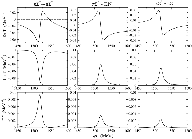
Figure 4: Unitary amplitudes involving the $\pi\Sigma^{*}$ channel. From left to right: $\pi\Sigma^{*}\to\pi\Sigma^{*}$, $\pi\Sigma^{*}\to\bar{K}N$ and $\pi\Sigma^{*}\to\pi\Sigma$.

It is worth mentioning that the unitarization procedure does not only provide the amplitude at the peak of the resonance but also obtains the full amplitude at energies away from it. This can have repercussion in some observables in specific physical processes as we will discuss below.

From the imaginary part of the amplitudes it is straightforward to obtain the couplings of the ${\Lambda(1520)}$ to the different channels in the following way. Close to the peak the amplitudes can be approximated by Eq. (10), which in this case reads

$$T_{ij}(\sqrt{s})=\frac{g_{i}g_{j}}{\sqrt{s}-M_{\Lambda(1520)}+i\Gamma_{\Lambda(1520)}/2}$$ (14)

from where we have

$$g_{i}g_{j}=-\frac{\Gamma_{\Lambda(1520)}}{2}\frac{|T_{ij}(M_{\Lambda(1520)})|^{2}}{Im[T_{ij}(M_{\Lambda(1520)})]},$$ (15)

where $M_{\Lambda(1520)}$ is the position of the peak in $|T_{ij}|^{2}$ and $\Gamma_{\Lambda(1520)}=15.6\textrm{ MeV}$.

Up to a global sign of one of the couplings (we choose $g_{1}$ to be positive), the couplings we obtain are shown in Table 2.

$g_{1}$	$g_{2}$	$g_{3}$	$g_{4}$
$0.91$	$-0.29$	$-0.54$	$-0.45$
$\pm 0.06$	$\pm 0.06$	$\pm 0.01$	$\pm 0.01$

Table 2: Couplings of the ${\Lambda(1520)}$ resonance to the different channels

We can see from the values that the ${\Lambda(1520)}$ resonance couples most strongly to the $\pi\Sigma^{*}$ channel. The fact that we are able to predict the value of this coupling is a non trivial consequence of the unitarization procedure that we employ.

In order to determine the errors in the $g_{i}$ couplings, we propagate the errors of Table 1 into Eq. (15). Another source of uncertainty arises from the fact that in the $\pi\Sigma^{*}$ and $K\Xi^{*}$ channels the maximum of $|T|^{2}$ and $ImT$ appear at slightly different energies (about $4\textrm{ MeV}$). This induces also some uncertainty in the evaluation of Eq. (15) and is also taken into account in the errors shown in Table 2.

With the value for $g_{1}$ obtained above, we now evaluate the partial decay width of the $\Lambda(1520)$ into $\pi\pi\Lambda$ assuming that this process is dominated by the $\pi\Sigma^{*}$ channel. The diagram describing this decay is shown in Fig. 5.

Figure 5: Diagram for ${\Lambda(1520)}$ decay into $\pi\pi\Lambda$

The amplitude for the decay can be written as

$$t(p_{1},p_{2})=\frac{g_{1}}{\sqrt{s_{\Sigma^{*}}}-M_{\Sigma^{*}}+i\Gamma_{\Sigma^{*}}(\sqrt{s_{\Sigma^{*}}})/2}\frac{f_{\Sigma^{*}\pi\Lambda}}{m_{\pi}}\langle\frac{1}{2}m|\vec{S}\cdot\vec{p_{2}}|\frac{3}{2}M\rangle,$$ (16)

where $\vec{p}_{2}$ is taken in the rest frame of the $\Sigma^{*}$. The width is then given by

$$\Gamma_{{\Lambda(1520)}\to\pi\pi\Lambda}=\frac{1}{2}\frac{1}{(2\pi)^{4}}\frac{M_{\Lambda}M_{{\Lambda(1520)}}}{4\sqrt{s}}\int_{-1}^{1} d\cos\theta_{1}\int_{m_{\pi}}^{\omega_{max}}d\omega_{1}\ \int_{0}^{2\pi}d{\tilde{\phi}}_{2}\ \int_{m_{\pi}}^{\omega_{max}}d\omega_{2}\cdot$$ (17)

$$\cdot \frac{1}{4}\sum_{m,M}|t(p_{1},p_{2})+t(p_{2},p_{1})|^{2}\ \Theta(1-|A|^{2})$$

where $A=\cos\theta_{12}=\frac{\left[(\sqrt{s}-\omega_{1}-\omega_{2})^{2}-|\vec{p}_{1}|^{2}-|\vec{p}_{2}|^{2}-M_{\Lambda}^{2}\right]}{2\ |\vec{p}_{1}||\vec{p}_{2}|}$ and $\omega_{max}=\frac{s+m_{\pi}^{2}-(m_{\pi}+M_{\Lambda})^{2}}{2\sqrt{s}}$.

With the coupling $g_{1}$ of Table 2, and dividing the result of Eq. (17) by 0.88 (the branching ratio of the $\Sigma(1385)$ decay into $\pi\Lambda$), we obtain a branching ratio for $\Lambda(1520)\to\pi\Sigma^{*}$ of around 0.14. By using the expression $Im\tilde{T}_{ij}=\sqrt{B_{i}B_{j}}$ we can see from Fig. 2 that the branching ratios for $\bar{K}N$ and $\pi\Sigma$ are $0.45$ and $0.43$ respectively. All these branching ratios essentially sum up to unity considering the uncertainties in the calculations, (in particular the exact position of the peak where the couplings are evaluated). The branching ratio to $\pi\Sigma^{*}$ is small because of lack of phase space for the decay. However, the relevant magnitude concerning the nature of a resonance is the coupling of the resonance to the different states. In this sense the $g_{1}$ coupling is still the largest. Originally, we had a theory with chiral Lagrangians which provided the $\Lambda(1520)$ as a dynamically generated resonance from $\pi\Sigma^{*}$. In reality also the $\bar{K}N$ and $\pi\Sigma$ channels are present, which are quite relevant and distort that approximate picture. As a consequence, $g_{1}$ becomes reasonably smaller and simultaneously one gets a relatively large $\bar{K}N$ and $\pi\Sigma$ coupling. Yet, with this admittedly large distortion of the original picture of the $\Lambda(1520)$ as a quasibound $\pi\Sigma^{*}$ state, the physical $\Lambda(1520)$ seems to keep a memory of this original picture which shows up in the coupling $g_{1}$, such that $g_{1}^{2}$ is $2.8$ times larger than the coupling squared for the $\bar{K}N$ state. This of course should manifest itself in processes where the $\pi\Sigma^{*}$ channel appears without restrictions of phase space, like in $\Lambda(1520)$ decay in nuclei in that channel with the pion becoming a $ph$ excitation.

The prediction of the amplitudes involving $\pi\Sigma^{*}$ channels can be checked in particular reactions where this channel could play an important role. First we evaluate the cross section for $K^{-}p\to\pi\pi\Lambda$ in the lines of Ref. [19] but using the new coupled channel formalism. The mechanisms and the expressions for the amplitudes and the cross sections can be found in Ref. [19] where, apart from the coupled channel unitarized amplitude, other mechanisms of relevance above the ${\Lambda(1520)}$ peak were included.

In Figs. 6 and 7 we show our results for $K^{-}p\to\pi^{0}\pi^{0}\Lambda$ and $K^{-}p\to\pi^{+}\pi^{-}\Lambda$ cross section respectively along with experimental data from Refs. [18, 17].

Figure 6: Result for the $K^{-}p\to\pi^{0}\pi^{0}\Lambda$ cross section. Experimental data from Ref. [18]

Figure 7: Result for the $K^{-}p\to\pi^{+}\pi^{-}\Lambda$ cross section. Experimental data from Ref. [17].

The dashed line represents the contribution from mechanisms other than the unitarized coupled channels, and the solid gives the coherent sum of all the processes. Note that the cross section of the $K^{-}p\to\pi^{+}\pi^{-}\Lambda$ reaction is a factor two larger at the peak than the $K^{-}p\to\pi^{0}\pi^{0}\Lambda$ one. These cross sections depend essentially on the $T_{\bar{K}N\to\pi\Sigma^{*}}$ amplitude, which is obtained from our coupled channel analysis. It is a non-trivial prediction of the theory since this amplitude has not been included in the fit. Actually, the strength at the peak comes essentially from the unitarity constraint of the theory in analogy with the discussion above regarding the $g_{1}$ coupling.

We now evaluate the $K^{-}p$ invariant mass distribution for the $\gamma p\to K^{+}K^{-}p$ reaction. In Ref. [42] the basic phenomenological model is explained but there only the $\pi\Sigma^{*}$ and $K\Xi^{*}$ channels were considered. The amplitude reads now

$$t_{\gamma p\to K^{+}K^{-}p}=V_{1}\sqrt{\frac{2}{3}}kG_{\pi\Sigma^{*}}T_{\pi\Sigma^{*}\to\bar{K}N}\left(\frac{-1}{\sqrt{2}}\right),$$ (18)

where $k$ is the photon energy and $V_{1}$ the $\gamma pK^{+}\pi\Sigma^{*}$ vertex function which we assume to have a smooth energy dependence. In Eq. (18) the last numerical factor is an isospin coefficient to project the $K^{-}p$ state into $I=0$. This amplitude is effectively written in such a way that when taking $|t|^{2}$ one is automatically summing and averaging over final and initial spin polarizations respectively. In Fig. 8 we present the results obtained with the formalism of the present work along with the experimental data of [43], where we have removed $50$ of the arbitrary units in the background which are apparent below the resonant peak. This background could be associated to the Drell mechanism ($K$ exchange in the $t$-channel), as discussed in [27]. Given the fact that the absolute strength of the results is a free parameter, the results do not change qualitatively if this background is not removed.

Figure 8: $K^{-}p$ invariant mass distribution for the $\gamma p\to K^{+}K^{-}p$ reaction with photons in the range $E_{\gamma}=2.8-4.8\textrm{ GeV}$. Experimental data from [43].

The normalization is arbitrary in the experimental data as well as in our calculation. For the purpose of the present work the shape of the distribution is the most important part and we can see that the agreement is quite fair. It is worth mentioning that in the work of Ref. [42] the reaction was initiated by a $\pi\Sigma^{*}$ loop. However, with the new channels considered in the present work, initial $\bar{K}N$ and $\pi\Sigma$ loops are also possible. The coupling of these channels to $\gamma pK^{+}$ can be different. However we have checked that the shape of the distribution for all these possibilities is very similar around the ${\Lambda(1520)}$ peak. For higher energies this is also true within about $30$%.

Note that for our purpose we do not need an explicit model for the photoproduction of the $\Lambda(1520)$, the $V_{1}$ term of Eq. (18). All we are stating is that there is a doorway for the production of the $\Lambda(1520)$ through the intermediate production of $\pi\Sigma(1385)$ (or $\bar{K}N$, $\pi\Sigma$, states). In the literature there are explicit models for the $\gamma N\to K\Lambda(1520)$ reaction. In one of them [27] it is shown that $K$ exchange in the $t$-channel cannot explain the data of Ref. [43] and consequently the weight of the cross section is put in $K^{*}$ exchange, for which the appropriate helicity amplitudes are parametrized to reproduce the data. However, the situation, as clearly stated in [27], is that the $\gamma p\to K^{+}\Lambda(1520)$ reaction can be more elaborate than assumed in their model, or other models, to the point that they could not provide a precise determination of the $K^{*}N\Lambda(1520)$ coupling. In Ref. [28], $s$- and $u$-channels plus a contact $\gamma NK\Lambda(1520)$ term are also introduced and a parametrization is used based on Regge trajectories. Two solutions are given for the $NK^{*}\Lambda(1520)$ coupling which, in terms of the $NK\Lambda(1520)$ one, was given by $\alpha g_{NK\Lambda(1520)}$, with $\alpha=0.37$ or $-0.66$, which gives us an idea of the strength of the coupling. However, in Ref. [44], a different parametrization of such terms is done, without using Regge trajectories, but introducing explicitly form factors, by means of which a good reproduction of the $\gamma p\to K^{+}\Lambda(1520)$ data is obtained which would be compatible with having a $NK^{*}\Lambda(1520)$ coupling equal zero, and the largest contribution comes from the contact term. In a more recent paper [45] the $K^{*}$ coupling to $N\Lambda(1520)$ is evaluated using the present model and a simple quark model for comparison. The coupling obtained in [45] with the present model is smaller than in the quark model and also than in [28]. As we can see from the previous discussion, the role of the $K^{*}$ exchange mechanism in the $\gamma p\to K^{+}\Lambda(1520)$ reaction is rather controversial. However, for the purpose of the present work this information is not needed. It would be absorbed in our $V_{1}$ term of Eq. (18) which is unnecessary in our comparison with the unnormalized cross section, or in ratios of cross sections as we discuss below.

In Ref. [42] it was suggested that the ratio of the $\pi^{0}\pi^{0}\Lambda$ mass distribution of the $\gamma p\to K^{+}\pi^{0}\pi^{0}\Lambda$ to the $K^{-}p$ distribution of the $\gamma p\to K^{+}K^{-}p$ reaction at the peak of the ${\Lambda(1520)}$ resonance can provide a test of the coupling of the ${\Lambda(1520)}$ to $\pi\Sigma^{*}$ ($g_{1}$). In an analogous way to the $K^{-}p\to\pi^{0}\pi^{0}\Lambda$ reaction, the $\gamma p\to K^{+}\pi^{0}\pi^{0}\Lambda$ would proceed through $\gamma p\to K^{+}\pi^{0}(\Sigma^{*})\to K^{+}\pi^{0}(\pi^{0}\Lambda)$. The amplitude is

$$t_{\gamma p\to K^{+}\pi^{0}\pi^{0}\Lambda}(p1,p2) = V_{1}\sqrt{\frac{2}{3}}kG_{\pi\Sigma^{*}}T_{\pi\Sigma^{*}\to\pi\Sigma^{*}}\frac{-1}{\sqrt{3}}\,\cdot$$ (19)

$$\cdot \frac{1}{\sqrt{s_{\Sigma^{*}}}-M_{\Sigma^{*}}+i\Gamma_{\Sigma^{*}}(\sqrt{s_{\Sigma^{*}}})/2}\frac{f_{\Sigma^{*}\pi\Lambda}}{m_{\pi}}\frac{1}{\sqrt{2}}(p_{2x}-ip_{2y}),$$

where one has to consider the same symmetrization arguments as in the $K^{-}p\to\pi^{0}\pi^{0}\Lambda$ reaction and $\vec{p}_{2}$ is taken in the rest frame of the $\Sigma^{*}$. Once again this amplitude is effectively written in such a way that when taking $|t|^{2}$ one is automatically summing and averaging over final and initial spin polarizations respectively. Up to phase space and the rest of numerical factors the ratio $R=(d\sigma_{\gamma p\to K^{+}\pi^{0}\pi^{0}\Lambda}/dM_{\pi^{0}\pi^{0}\Lambda})/(d\sigma_{\gamma p\to K^{+}K^{-}p}/dM_{K^{-}p})$ is proportional to $(|T_{\pi\Sigma^{*}\to\pi\Sigma^{*}}|/|T_{\pi\Sigma^{*}\to\bar{K}N}|)^{2}$ which, at the ${\Lambda(1520)}$ peak position, is $(g_{1}/g_{3})^{2}$ (see Eq. (14)). All considered we obtain a value for the ratio of $R\sim 0.25\pm 0.04$, while $(g_{1}/g_{3})^{2}$ is $2.8$, where the error of $R$ has been obtained propagating the errors of Table 2.

In Fig 8 we see that our model seems to be lacking some strength at energies below the $\Lambda(1520)$ peak. This could be due to lack of some background terms or the large uncertainty of the experimental errors. In fact, it is worth stressing that the same feature appears in the result of Ref. [27]. On the other hand, more recent experimental results [46] and [47], although at different photon energies, do not show this broad shoulder.

Next we show, in Fig. 9, the $K^{-}p$ invariant mass distribution for the $\pi^{-}p\to K^{0}K^{-}p$ reaction. The model used for this purpose is analogous to the one used in the study of the $\gamma p\to K^{+}K^{-}p$ reaction. The differences are in the phase space and in the first vertex where we have used a different unknown constant.

Figure 9: $K^{-}p$ invariant mass distribution for the $\pi^{-}p\to K^{0}K^{-}p$ reaction. Left plot: pions in the range $p_{\pi^{-}}=1.6-2.4\textrm{ GeV/c}$; right plot: $p_{\pi^{-}}=2.9-3.3\textrm{ GeV/c}$. Experimental data from Ref. [48].

In Ref. [48] no errors in the experimental data are provided, hence we have assumed errors to be the square root of the number of events (statistical errors). We see that the agreement is fair considering the large experimental errors. Note that, unlike in the case of photoproduction, we did not subtract a background here, which would clearly make the agreement with experiment better at energies below the $\Lambda(1520)$ region.

4 Conclusions

We have done a coupled channel analysis of the ${\Lambda(1520)}$ resonance using the $\pi\Sigma(1385)$, $K\Xi(1530)$, $\bar{K}N$ and $\pi\Sigma$ channels. We have used the Bethe-Salpeter equation to implement unitarity in the evaluation of the different amplitudes. The main novelty from previous coupled channel approaches to this resonance is the inclusion of new matrix elements in the kernel of the BS equation and the consideration of the $\Sigma(1385)$ width in the $\pi\Sigma^{*}$ loop function. The unknown parameters in the $V-$matrix, as well as the subtraction constants of the loop functions, have been obtained by a fit to $\bar{K}N\to\bar{K}N$ and $\bar{K}N\to\pi\Sigma$ partial wave amplitudes. As a consequence of the unitarity of the scheme used, we can predict the amplitudes and couplings of the ${\Lambda(1520)}$ for all the different channels. The largest coupling is obtained for the $\pi\Sigma^{*}$ channel.

We have then tested the amplitudes obtained in several specific reactions and compared with experimental data at energies close to and slightly above the ${\Lambda(1520)}$ region. These include the $K^{-}p\to\Lambda\pi\pi$, $\gamma p\to K^{+}K^{-}p$, $\gamma p\to K^{+}\pi^{0}\pi^{0}\Lambda$ and $\pi^{-}p\to K^{0}K^{-}p$ reactions. We have obtained a reasonable agreement with the experimental results that allows us to be confident in the procedure followed to describe the nature of the ${\Lambda(1520)}$ resonance.

For the $K^{-}p\to\Lambda\pi\pi$ process, both with neutral and charged pions, we could do predictions of the absolute cross sections since the process involves the amplitude for the $K^{-}p\to\pi\Sigma^{*}$ transition, which is an output of our theory. In the other two cases the strength of the cross section was left as a free parameter since no theory was done for the coupling of the photon or the pion to the $\Lambda(1520)$ components. Yet, it was found that in all cases the shape of the resonance was rather asymmetric, with a substantial strength above the peak of the resonance in all the reactions, which seems to be an intrinsic property of the $\Lambda(1520)$ resonance, and which in our theoretical framework could be attributed to the $d$-wave character of the $\bar{K}N$ and $\pi\Sigma$ channels, as well as to the fact that above the resonance peak the phase space for the $\Lambda(1520)$ decay into the $\pi\Sigma^{*}$ channel grows rapidly.

We could see that, in spite of the relevant role played by the $\bar{K}N$ and $\pi\Sigma$ channels, the $\Lambda(1520)$ remains with the largest coupling to the $\pi\Sigma^{*}$ channel. In a simplified theory in which only the $s$-wave $\pi\Sigma^{*}$ and $K\Xi^{*}$ channels are taken, and their interaction is provided by the chiral Lagrangians, the $\Lambda(1520)$ appears naturally and qualifies as a quasibound $\pi\Sigma^{*}$ state. The coupling of the resonance to the $\bar{K}N$ and $\pi\Sigma$ channels in the real world modifies appreciably this picture but the state still keeps memory of the original simplified picture and has still a large coupling to $\pi\Sigma^{*}$ with a strength of $g^{2}$ of the order of three times larger than that of the $\bar{K}N$ or $\pi\Sigma$ channels.

Further tests to show the dominance of the $\pi\Sigma^{*}$ component in the $\Lambda(1520)$ resonance could be done, in particular a crucial test would be the modification of the $\Lambda(1520)$ width in nuclei, and particularly the $\pi\Sigma^{*}$ mode that in nuclei would give rise to the $ph\Sigma^{*}$ decay channel. In this way one could observe a drastically enhanced production of $\Sigma^{*}$ in processes involving $\Lambda(1520)$ decay in nuclei, while at the same time one would observe an increased $\Lambda(1520)$ width in other physical processes. The understanding of the nature of this resonance and the comprehension of processes where the resonance appears would benefit much from the performance of such experiments.

References

- [1] T. Nakano, talk at the Pentaquark04 meeting http://www.rcnp.osaka-u.ac.jp/ penta04/
- [2] K. Joo et al. [CLAS Collaboration], Phys. Rev. C 72 (2005) 058202.
- [3] N. Kaiser, T. Waas and W. Weise, Nucl. Phys. A 612 (1997) 297.
- [4] E. Oset and A. Ramos, Nucl. Phys. A 635 (1998) 99.
- [5] J. A. Oller and U. G. Meissner, Phys. Lett. B 500 (2001) 263.
- [6] C. Garcia-Recio, J. Nieves, E. Ruiz Arriola and M. J. Vicente Vacas, Phys. Rev. D 67 (2003) 076009.
- [7] T. Hyodo, A. Hosaka, E. Oset, A. Ramos and M. J. Vicente Vacas, Phys. Rev. C 68 (2003) 065203.
- [8] J. A. Oller, E. Oset and A. Ramos, Prog. Part. Nucl. Phys. 45 (2000) 157.
- [9] D. Jido, J. A. Oller, E. Oset, A. Ramos and U. G. Meissner, Nucl. Phys. A 725 (2003) 181.
- [10] C. Garcia-Recio, M. F. M. Lutz and J. Nieves, Phys. Lett. B 582 (2004) 49.
- [11] S. Prakhov et al. [Crystall Ball Collaboration], Phys. Rev. C 70 (2004) 034605.
- [12] D. W. Thomas, A. Engler, H. E. Fisk and R. W. Kraemer, Nucl. Phys. B 56 (1973) 15.
- [13] V. K. Magas, E. Oset and A. Ramos, Phys. Rev. Lett. 95 (2005) 052301.
- [14] E. E. Kolomeitsev and M. F. M. Lutz, Phys. Lett. B 585 (2004) 243.
- [15] S. Sarkar, E. Oset and M. J. Vicente Vacas, Nucl. Phys. A 750 (2005) 294.
- [16] S. Eidelman et al. [Particle Data Group], Phys. Lett. B 592, 1 (2004).
- [17] T. S. Mast, M. Alston-Garnjost, R. O. Bangerter, A. Barbaro-Galtieri, F. T. Solmitz and R. D. Tripp, Phys. Rev. D 7 (1973) 5.
- [18] S. Prakhov et al., Phys. Rev. C 69 (2004) 042202.
- [19] S. Sarkar, E. Oset and M. J. Vicente Vacas, Phys. Rev. C 72 (2005) 015206.
- [20] A. Dobado and J. R. Pelaez, Phys. Rev. D 56 (1997) 3057.
- [21] J. A. Oller, E. Oset and J. R. Pelaez, Phys. Rev. D 59 (1999) 074001 [Erratum-ibid. D 60 (1999) 099906].
- [22] J. A. Oller and E. Oset, Phys. Rev. D 60 (1999) 074023.
- [23] J. A. Oller and E. Oset, Nucl. Phys. A 620 (1997) 438 [Erratum-ibid. A 652 (1999) 407].
- [24] F. Mandl and G. Shaw, Quantum Field Theory, Wiley-Interscience, 1984.
- [25] A. Ramos, E. Oset and C. Bennhold, Phys. Rev. Lett. 89 (2002) 252001.
- [26] E. Oset, A. Ramos and C. Bennhold, Phys. Lett. B 527 (2002) 99 [Erratum-ibid. B 530 (2002) 260].
- [27] A. Sibirtsev, J. Haidenbauer, S. Krewald, U. G. Meissner and A. W. Thomas, arXiv:hep-ph/0509145.
- [28] A. I. Titov, B. Kampfer, S. Date and Y. Ohashi, Phys. Rev. C 72 (2005) 035206 [Erratum-ibid. C 72 (2005) 049901] [arXiv:nucl-th/0506072].
- [29] U. G. Meissner and J. A. Oller, Nucl. Phys. A 673 (2000) 311.
- [30] A. L. Fetter and J. D. Walecka, Quantum Theory of Many Particle Systems (McGraw-Hill, New York, 1971)
- [31] N. Fettes and U. G. Meissner, Nucl. Phys. A 679 (2001) 629.
- [32] B. Borasoy, R. Nissler and W. Weise, Eur. Phys. J. A 25 (2005) 79.
- [33] J. A. Oller, J. Prades and M. Verbeni, Phys. Rev. Lett. 95 (2005) 172502.
- [34] V. Bernard, H. W. Fearing, T. R. Hemmert and U. G. Meissner, Nucl. Phys. A 635 (1998) 121 [Erratum-ibid. A 642 (1998 NUPHA,A642,563-563.1998) 563] [arXiv:hep-ph/9801297].
- [35] J. Gasser and A. Zepeda, Nucl. Phys. B 174 (1980) 445.
- [36] N. Fettes, U. G. Meissner and S. Steininger, Nucl. Phys. A 640 (1998) 199.
- [37] G. Ecker, J. Gasser, A. Pich and E. de Rafael, Nucl. Phys. B 321 (1989) 311.
- [38] E. Jenkins and A. V. Manohar, Phys. Lett. B 259 (1991) 353.
- [39] G. P. Gopal, R. T. Ross, A. J. Van Horn, A. C. McPherson, E. F. Clayton, T. C. Bacon and I. Butterworth [Rutherford-London Collaboration], Nucl. Phys. B 119 (1977) 362.
- [40] M. Alston-Garnjost, R. W. Kenney, D. L. Pollard, R. R. Ross, R. D. Tripp, H. Nicholson and M. Ferro-Luzzi, Phys. Rev. D 18 (1978) 182.
- [41] R. Guardiola, E. Higon and J. Ros, Metodes numerics per a la fisica, Ed. Universitat de Valencia, 1995.
- [42] L. Roca, E. Oset and H. Toki, arXiv:hep-ph/0411155.
- [43] D. P. Barber et al., Z. Phys. C 7 (1980) 17.
- [44] S. I. Nam, A. Hosaka and H. C. Kim, Phys. Rev. 71 (2005) 114012.
- [45] T. Hyodo, S. Sarkar, A. Hosaka and E. Oset, [arXiv:hep-ph/0601026].
- [46] J. Barth et al. [SAPHIR Collaboration], Phys. Lett. B 572 (2003) 127 ; J. Barth et al., Eur. Phys. J. A 17 (2003) 269.
- [47] N. A. Baltzel, in the NSTAR05 Workshop, Tallahassee, October 2005, http://hadron.physics.fsu.edu/NSTAR2005/.
- [48] O. I. Dahl, L. M. Hardy, R. I. Hess, J. Kirz, D. H. Miller and J. A. Schwartz, Phys. Rev. 163 (1967) 1377.