Large next-to-leading order QCD corrections to pentaquark sum rules

Abstract

Using configuration space techniques, we calculate next-to-leading order (NLO) five-loop QCD corrections to the correlators of interpolating pentaquark currents in the limit of massless quarks. We obtain very large NLO corrections to the spectral density which makes a standard sum rule analysis problematic. However, the NLO corrections to the correlator in configuration space are reasonable. We discuss the implications of our results for the phenomenological sum rule analysis of pentaquark states.

I Introduction

There is a continuing interest in exotic states of strong interactions that differ from the standard nonexotic mesons and baryons (see e.g. Matveev ; Braun:1988kv ). Nonexotic three-quark baryons have been intensively studied in  Ioffe ; Chung . Finite mass effects were studied in Pivovarov:1988gt ; Ovchinnikov ; Groote where the next-to-leading order (NLO) QCD corrections to the correlators of finite mass baryonic currents were determined. This led to an improved precision of the sum rule analysis. Different aspects of the physics of multiquark states in QCD have been discussed long ago Larin:1985yt . It is noteworthy that the analysis of multiquark exotics can provide valuable information on the details of quark-gluon interaction relevant to nuclear physics Meissner:2004yy ; Bijnens:2005mi .

Candidates to be described in QCD as multiquark states are the deuteron LarMat ; Kulagin:kb or Jaffe’s dihyperon $H$ Jaffe ; Sakai:1999qm . Since the dihyperon state can only decay weakly, it would be expected to be quite narrow. To the best of our knowledge the dihyperon state is the first state to attract attention in the modern context of QCD. The discovery of gluon bound states would be a triumphant confirmation of QCD and would allow for a quantitative check of QCD in the completely new sector of the glueball states Brodsky:2003hv ; Kataev:1981aw . Another class of multiquark states, the pentaquark states, have recently become the focus of intense theoretical and experimental studies.

The properties of all of these multiquark (or multigluon) states can be studied in a model independent way through the method of the QCD sum rule analysis. In the QCD sum rule analysis one analyzes the operator product expansion of current–current correlators of interpolating local fields which have the quantum numbers of the multiquark states under study. It is well known that radiative corrections have a strong impact on the results of the sum rule analysis. In this paper we derive the necessary tools that allow one to compute the $\alpha_{S}$ radiative corrections to multiquark sum rules in the limit when the quarks (or antiquarks) are massless. As a specific example we apply our method to pentaquark correlators and calculate the NLO radiative corrections to the pentaquark current correlator and the spectral density of a specific pentaquark current.

II Calculation

An important ingredient in the formulation of the operator product expansion (OPE) analysis for the pentaquark states is the choice of the interpolating current. The result depends strongly on the choice of the interpolating current as has been pointed out before in the sum rule analysis of the dibaryon Larin:1985yt . The same holds true for the sum rule analysis of pentaquark states Matheus:2004qq ; Matheus:2004gx ; Lee:2005ny . A detailed analysis of the dependence on the interpolating current is out of the scope of a short letter, it will be published elsewhere Groote:2006 . In the following we shall present the tools needed to calculate the NLO QCD corrections for interpolating quark currents of any composition.

II.1 Generalities

In the QCD sum rule analysis the prime object of study is the correlation function

$$\Pi(q)=i\int d^{4}xe^{iqx}\langle 0|Tj(x)\bar{j}(0)|0\rangle,$$ (1)

where the interpolating current $j(x)$ is a local operator with the quantum numbers of the pentaquark baryon state $\Theta$. It has to be constructed from four quark and one antiquark fields such that its projection onto the pentaquark state $|\Theta(p)\rangle$ is nonzero:

$$\langle 0|j(0)|\Theta(p)\rangle=\lambda_{\Theta},\quad p^{2}=m_{\theta}^{2}.$$ (2)

Since the interpolating current $j(x)$ is not unique, one immediately faces the question of the optimal choice for the interpolating currents. Recall that the problem of choosing the optimal current already arose in the case of baryons Ioffe ; Chung where the currents are constructed from three quark fields. In the pentaquark case there are five quark (antiquark) fields to build the interpolating currents and correspondingly the number of independent currents with the correct quantum numbers is much larger (see Matheus:2004gx and references therein).

The treatment of the interpolating current $j(x)$ in its most general form, i.e. in the form of linear combinations of all possible independent local operators with the correct pentaquark quantum numbers, is a very unwieldy problem. In this pilot study of the NLO corrections to interpolating pentaquark currents we limit ourselves to the study of only one simple interpolating currents with the required pentaquark quantum numbers. As in the case of mesons and baryons, we construct our interpolating current $j(x)$ from quark fields without derivatives.

II.2 Tools for the NLO calculation

The LO diagram for the pentaquark correlator is given by the four-loop diagram FIG. 1(a).

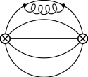
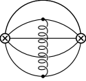
(a)(b)(c)

Figure 1: LO contribution (a) and examples for the NLO propagator (b) and dipropagator corrections (c)

There are two types of NLO five-loop corrections. First there are the one-loop corrections to single quark propagators $S(x)$, one of which is shown in FIG. 1(b). We shall refer to these corrections as the propagator corrections. Then there are the dipropagator corrections connecting two different quark propagators, one of which is shown in FIG. 1(c).

It turns out that it is very convenient to calculate these corrections in configuration space, in particular if the quarks are treated as massless Groote:2005ay . For the propagator correction $S_{1}(x)$ we obtain

$$S_{1}(x)|_{\rm NLO} = S_{1}(x)|_{\rm LO}\left\{1-C_{F}\frac{\alpha_{s}}{4\pi}\frac{1}{\varepsilon}\left(\mu^{2}_{X}x^{2}\right)^{\varepsilon}\right\}$$ (3)

$$= S_{0}(x^{2})\gamma^{\mu}x_{\mu}\left\{1-C_{F}\frac{\alpha_{s}}{4\pi}\frac{1}{\varepsilon}\left(\mu^{2}_{X}x^{2}\right)^{\varepsilon}\right\}$$

where in the Euclidean domain one has

$$S_{0}(x^{2})=\frac{-i\Gamma(2-\varepsilon)}{2\pi^{2-\varepsilon}(x^{2})^{2-\varepsilon}}.$$ (4)

$\mu_{X}$ is a renormalization scale in dimensional regularization appropriate for calculations in configuration space. The space-time dimension is parametrized by $D=4-2\varepsilon$. This choice of renormalization scale avoids the appearance of $\ln(4\pi)$ and $\gamma_{E}$ factors in configuration space calculations. The relation of $\mu_{X}$ and the usual renormalization scale $\mu$ of the $\overline{\mbox{MS}}$-scheme is given by

$$\mu_{X}=\mu e^{\gamma_{E}}/2.$$

The dipropagator two-loop amplitude for a pair of quarks with open Dirac indices leads to an integral that is a bit more difficult to calculate. The result for the dipropagator correction including the LO term reads

$$S_{2}(x)|_{\rm NLO}\ =\ S_{0}(x^{2})^{2}\{\gamma^{\mu}x_{\mu}\otimes\gamma^{\nu}x_{\nu}$$ (5)

$$+t^{a}\otimes t^{a}\frac{\alpha_{s}}{4\pi}\frac{1}{\varepsilon}(\mu_{X}^{2}x^{2})^{\varepsilon}(\gamma^{\mu}\otimes\gamma^{\nu}(a_{1}x_{\mu}x_{\nu}+b_{1}x^{2}g_{\mu\nu})$$

$$\qquad\qquad\qquad\qquad+a_{3}\Gamma_{3}^{\alpha\beta\mu}\otimes{\Gamma_{3\ \alpha\beta}}^{\nu}x_{\mu}x_{\nu})\}$$

where the coefficients $a_{1}$, $b_{1}$ and $a_{3}$ are given by

$$a_{1}=-1-\frac{11}{2}\varepsilon,\quad b_{1}=-1-\frac{1}{2}\varepsilon,\quad a_{3}=-\frac{1}{2}-\frac{1}{4}\varepsilon,$$

and where

$$\Gamma_{3}^{\mu\alpha\nu}=\frac{1}{2}(\gamma^{\mu}\gamma^{\alpha}\gamma^{\nu}-\gamma^{\nu}\gamma^{\alpha}\gamma^{\mu}).$$ (6)

Eqs. (3) and (5) allow one to calculate the NLO corrections to $n$-quark(antiquark) current correlators of any composition using purely algebraically algorithms without having to compute any integrals.

II.3 Renormalization of the interpolating current

In a NLO calculation one has to account for mixing effects between operators when going through the renormalization program. Mixing can occur when gluons are exchanged between the lines in the pentaquark correlator (dipropagator corrections). In order to keep track of flavours we first treat the case of an interpolating current composed of five massless quark(antiquark) fields with different flavours,

$$j=\varepsilon^{ijk}(q_{1}^{iT}Cq_{2}^{j})q_{3}^{k}(\bar{q}_{4}^{l}q_{5}^{l})$$ (7)

where $C$ is the charge conjugation matrix. The interpolating current consists of a baryonic part $B=\varepsilon^{ijk}(q_{1}^{iT}Cq_{2}^{j})q_{3}^{k}$ and a mesonic part $M=(\bar{q}_{4}^{l}q_{5}^{l})$. If the gluon is exchanged within the mesonic part, the renormalization factor is the usual one for the mesonic operator (see e.g. Pivovarov:1991nk ),

$$Z_{M}=1-\frac{\alpha_{s}}{\pi\varepsilon}.$$ (8)

If the gluon is exchanged within the baryonic part, the renormalization factor is given by the known renormalization factor for the baryonic operator Pivovarov:1991nk ,

$$Z_{B}=1-\frac{\alpha_{s}}{2\pi\varepsilon}.$$ (9)

These two contributions will be referred to as factorizing contributions. When the gluon is exchanged between the mesonic and baryonic part one obtains new operators which do not have the structure of the original current. There are two contributions of this kind which we refer to as mixed contributions. If the gluon is exchanged between the mesonic part and the $(q_{1}^{iT}Cq_{2}^{j})$ piece of the baryonic part, we obtain a contribution of the operator

$$O_{1}=\varepsilon^{ijk}\Big{\{}(q_{1}^{iT}C\sigma^{\alpha\beta}q_{2}^{l})+(q_{1}^{lT}C\sigma^{\alpha\beta}q_{2}^{i})\Big{\}}q_{3}^{k}(\bar{q}_{4}^{l}\sigma^{\alpha\beta}q_{5}^{j})$$ (10)

where $\sigma^{\alpha\beta}=\frac{i}{2}[\gamma^{\alpha},\gamma^{\beta}]$. If the gluon is exchanged between the mesonic part and the $q_{3}^{k}$ piece of the baryonic part one obtains a contribution of the operator

$$O_{2}=\varepsilon^{ijk}(q_{1}^{iT}Cq_{2}^{j})\sigma^{\alpha\beta}\Big{\{}q_{3}^{l}(\bar{q}_{4}^{l}\sigma_{\alpha\beta}q_{5}^{k})-\frac{1}{3}q_{3}^{k}(\bar{q}_{4}^{l}\sigma_{\alpha\beta}q_{5}^{l})\Big{\}}.$$ (11)

The renormalized current reads

$$j_{R}^{\rm NLO}=Z_{M}Z_{B}j^{\rm NLO}-\frac{\alpha_{s}}{16\pi\varepsilon}\left(O_{1}+O_{2}\right).$$ (12)

III NLO results

In order to obtain NLO results, let us consider the interpolating current

$$j=\varepsilon^{abc}(u^{aT}Cd\,^{b})d\,^{c}(\bar{s}\,^{e}u^{e})$$ (13)

with the quantum numbers of the pentaquark baryon $\Theta$. The current is constructed in such a way that it cannot directly dissociate into a neutron and a kaon since the respective color singlet parts have the wrong parity.

The result of our NLO calculation for the bare correlator reads $(\bar{j}=\varepsilon^{abc}(\bar{d}\,^{a}C^{-1}\bar{u}^{bT})\bar{d}\,^{c}(\bar{u}^{e}s^{e}))$

$$\langle 0|Tj(x)\bar{j}(0)|0\rangle=S_{0}(x^{2})^{5}(x^{2})^{2}\gamma^{\mu}x_{\mu}\Pi(x^{2})$$ (14)

where

$$\Pi(x^{2}) = 360\left(1+\frac{\alpha_{s}}{\pi}(\mu_{X}^{2}x^{2})^{\varepsilon}\left(\frac{3}{\varepsilon}+3\right)\right)$$ (15)

$$-6\left(1+\frac{\alpha_{s}}{\pi}(\mu_{X}^{2}x^{2})^{\varepsilon}\left(\frac{11}{\varepsilon}-\frac{7}{3}\right)\right)$$

$$-4\cdot 6\left(1+\frac{\alpha_{s}}{\pi}(\mu_{X}^{2}x^{2})^{\varepsilon}\left(\frac{9}{\varepsilon}-1\right)\right).$$

The first line contains the factorizing NLO contibutions while the second and third lines contain the mixing contributions. The counter term contains contributions from the renormalization factors $Z_{M}$ and $Z_{B}$ as well as from the operators $O_{1}$ and $O_{2}$. It reads

$$\Delta\Pi=-\frac{\alpha_{s}}{\pi}\left\{360\frac{3}{\varepsilon}-6\left(\frac{11}{\varepsilon}-\frac{28}{3}\right)-4\cdot 6\left(\frac{9}{\varepsilon}-7\right)\right\}.$$ (16)

Adding Eqs. (15) and (16) one obtains the renormalized correlator

$$\Pi_{R}(x^{2})\ =\ \Pi(x^{2})+\Delta\Pi\ =\ 360\left(1+\frac{\alpha_{s}}{\pi}\left(3+3L_{x}\right)\right)$$

$$-6\left(1+\frac{\alpha_{s}}{\pi}\left(7+11L_{x}\right)\right)-4\cdot 6\left(1+\frac{\alpha_{s}}{\pi}\left(6+9L_{x}\right)\right)$$

with $L_{x}=\ln(x^{2}\mu_{X}^{2})=\ln(x^{2}e^{2\gamma_{E}}/4)$.

The spectral density is obtained by calculating the discontinuity of

$$2\pi^{2-\varepsilon}\int_{0}^{\infty}\left(\frac{px}{2}\right)^{\varepsilon-1}J_{1-\varepsilon}(px)(x^{2})^{-a}x^{3-2\varepsilon}dx$$ (18)

for the cases $a=7$ and $a=7-\varepsilon$, where $J_{\lambda}(z)$ is the Bessel function of the first kind Groote:2005ay . One obtains ($s=p^{2}$)

$$\rho(s)/\rho_{0}(s) = 360\left(1+\frac{\alpha_{s}}{\pi}\left(\frac{617}{35}+3L\right)\right)$$ (19)

$$-6\left(1+\frac{\alpha_{s}}{\pi}\left(\frac{6367}{105}+11L\right)\right)$$

$$-4\cdot 6\left(1+\frac{\alpha_{s}}{\pi}\left(\frac{1746}{35}+9L\right)\right)$$

with $L=\ln(\mu^{2}/s)$ and $\rho_{0}(s)=s^{5}/378000(4\pi)^{8}$.

IV Discussion

The first NLO contribution in both the correlator and the spectral density comes from the factorizing part of the diagrams, i.e. the case where baryon and meson correlators are multiplied in configuration space and do not mix by gluon exchange. This contribution dominates the final result but is probably irrelevant for physics as it does not contain a pentaquark bound state. The physically relevant mixing contributions are smaller since they are suppressed both in the number of colours $N_{c}$ and a factor $4$ coming from the evaluation of Dirac traces.

The result for the spectral density (19) shows that the NLO corrections to the spectral density are large, where the NLO corrections to the factorizing parts are somewhat smaller (note, however, that the relevant scale is not $s$ but rather $s/5$ because of the number of lines in the correlator). This spoils the conventional momentum space QCD sum rule analysis. The NLO corrections to the correlator function (III) in configuration space are more reasonable. This suggests a sum rule analysis in configuration space, based on the correlator (III). However, it is not clear whether the accuracy of such a sum rule analysis in configuration space will be sufficient for physical applications.

V Conclusion

We have calculated NLO perturbative QCD corrections for pentaquark current correlators which turn out to be very large. One has to conclude that the NLO QCD sum rule analysis of pentaquark states is fraught with difficulties. This complicates the mass determination of the pentaquark states using a QCD sum rule analysis. One may have to take recourse to model calculations to determine the properties of pentaquark states such as the one based on chiral solitons Diakonov:1997mm .

- (1) V.A. Matveev and P. Sorba, Lett. Nuovo Cim. 20 (1977) 435; R.L. Jaffe, Phys. Rev. D15 (1977) 267; P.J. Mulders, Phys. Rev. D25 (1982) 1269; E.L. Lomon, Phys. Rev. D26 (1982) 576; A.T.M. Aerts and C.B. Dover, Nucl. Phys. B253 (1985) 116
- (2) V.M. Braun and Y.M. Shabelski, Sov. J. Nucl. Phys. 50 (1989) 306 [Yad. Fiz. 50 (1989) 493]
- (3) B.L. Ioffe, Nucl. Phys. B188 (1981) 317 [Erratum-ibid. B191 (1981) 591]
- (4) Y. Chung, H.G. Dosch, M. Kremer and D. Schall, Nucl. Phys. B197 (1982) 55; D. Espriu, P. Pascual and R. Tarrach, Nucl. Phys. B214 (1983) 285
- (5) A.A. Pivovarov and R. Surguladze, Yad. Fiz. 48 (1988) 1856 [Sov. J. Nucl. Phys. 48 (1989) 1117]
- (6) A.A. Ovchinnikov, A.A. Pivovarov and L.R. Surguladze, Int. J. Mod. Phys. A6 (1991) 2025; Yad. Fiz. 48 (1988) 562 [Sov. J. Nucl. Phys. 48 (1988) 358]
- (7) S. Groote, J.G. Körner and A.A. Pivovarov, Phys. Rev. D61 (2000) 071501(R); in Batavia 2000, Advanced computing and analysis techniques in physics research pp. 277–279 [arXiv:hep-ph/0009218]
- (8) S.A. Larin, V.A. Matveev, A.A. Ovchinnikov and A.A. Pivovarov, Yad. Fiz. 44 (1986) 1066 [Sov. J. Nucl. Phys. 44 (1986) 690]
- (9) U.G. Meissner, Nucl. Phys. A751 (2005) 149
- (10) J. Bijnens, U.G. Meissner and A. Wirzba, “Effective field theories in nuclear, particle and atomic physics” [arXiv:hep-ph/0502008]
- (11) S.A. Larin and V.A. Matveev, Phys. Lett. B159 (1985) 62
- (12) S.A. Kulagin and A.A. Pivovarov, Yad. Fiz. 45 (1987) 952
- (13) R.L. Jaffe, Phys. Rev. Lett. 38 (1977) 195 [Erratum-ibid. 38 (1977) 617]
- (14) T. Sakai, K. Shimizu and K. Yazaki, Prog. Theor. Phys. Suppl. 137 (2000) 121
- (15) S.J. Brodsky, A.S. Goldhaber and J. Lee, Phys. Rev. Lett. 91 (2003) 112001
- (16) A.L. Kataev, N.V. Krasnikov and A.A. Pivovarov, Phys. Lett. B107 (1981) 115; Nucl. Phys. B198 (1982) 508 [Erratum-ibid. B490 (1997) 505]
- (17) R.D. Matheus and S. Narison, “Are the pentaquark sum rules reliable?” [arXiv:hep-ph/0412063]
- (18) R.D. Matheus, F.S. Navarra, M. Nielsen and R.R. da Silva, Phys. Lett. B602 (2004) 185
- (19) H.J. Lee, N.I. Kochelev and V. Vento, Phys. Rev. D73 (2006) 014010
- (20) S. Groote, J.G. Körner and A.A. Pivovarov, to appear.
- (21) Configuration space integration techniques are reviewed in S. Groote, J.G. Körner and A.A. Pivovarov, “On the evaluation of a certain class of Feynman diagrams in x-space: Sunrise-type topologies at any loop order”, submitted to Annals of Physics [arXiv:hep-ph/0506286]; Phys. Lett. B443 (1998) 269; Nucl. Phys. B542 (1999) 515; Eur. Phys. J. C11 (1999) 279
- (22) A.A. Pivovarov and L.R. Surguladze, Nucl. Phys. B360 (1991) 97
- (23) D. Diakonov, V. Petrov and M.V. Polyakov, Z. Phys. A359 (1997) 305