UdeM-GPP-TH-06-145
Hadronic Decays: A General Approach
Maxime Imbeault a,111maxime.imbeault@umontreal.ca, Alakabha Datta b,222datta@physics.utoronto.ca, and David London a,333london@lps.umontreal.ca
: Physique des Particules, Université
de Montréal,
C.P. 6128, succ. centre-ville, Montréal, QC,
Canada H3C 3J7
: Department of Physics, University of Toronto,
60 St. George Street, Toronto, ON, Canada M5S
1A7
()
Abstract
In this paper, we propose a general approach
for describing hadronic decays. Using this method, all amplitudes
for such decays can be expressed in terms of contractions, though the
matrix elements are not evaluated. Many years ago, Buras and
Silvestrini proposed a similar approach. However, our technique goes
beyond theirs in several ways. First, we include recent theoretical
and experimental developments which indicate which contractions are
negligible, and which are expected to be smaller than others. Second,
we show that all -decay diagrams can be simply expressed in terms
of contractions. This constitutes a formal proof that the diagrammatic
method is rigourous. Third, we show that one reproduces the relations
between tree and electroweak-penguin diagrams described by Neubert and
Rosner, and by Gronau, Pirjol and Yan. Fourth, although the previous
results hold to all orders in , we show that it is also
possible to work order-by-order in this approach. In this way it is
possible to make a connection with the matrix-element evaluation
methods of QCD factorization (QCDfac) and perturbative QCD (pQCD).
Finally, using the contractions approach, we re-evaluate the question
of whether there is a “ puzzle.” At , we
find that the diagram ratio is about 0.17, a factor of 10
too small to explain all the data. Both QCDfac and pQCD find
that, at , the value of may be raised to only
about 2-3 times its lowest-order value. We therefore conclude that,
assuming the effect is not a statistical fluctuation, it is likely
that the value of is similar to its result,
and that there really is a puzzle.
1 Introduction
The study of hadronic decays444In this paper, we present results for mesons, which contain a quark. We will nevertheless continue to refer to decays. has a long and storied history. Much work has gone into all aspects of this problem.
One important development was the operator-product expansion (OPE). Here the effective Hamiltonian for quark-level decays takes the form [1]
| (1) |
where . is the renormalization point, typically taken to be . The Wilson coefficients (WC’s) include gluons (QCD corrections) whose energy is above (short distance), while the operators include QCD corrections of energy less than (long distance). All physical quantities must be independent of . Note: factors of are omitted for the remainder of this paper.
The operators take the following form:
| (2) |
summed over colour indices and . These are the usual (tree-level) current–current operators induced by -boson exchange.
| , | |||||
| , | (3) |
summed over the light flavors . These are referred to as QCD penguin operators.
| , | |||||
| , | (4) |
with denoting the electric charges of the quarks. These are called electroweak-penguin (EWP) operators. The quark current denotes . All quark-level decays can be expressed in terms of the effective Hamiltonian.
An alternative description is the diagrammatic approach [2], in which quark-level decays are characterized by various topologies. These include the colour-favored and colour-suppressed tree amplitudes and , the gluonic penguin amplitude , the colour-favored and colour-suppressed EWP amplitudes and , the exchange diagram , the annihilation amplitude , and the penguin-annihilation diagram . This formalism has been extensively used, but the relation to the OPE and the effective Hamiltonian has not been made entirely clear.
Of course, the true decays involve mesons, and do not take place at the quark level. That is, the decay is , where is a charged or neutral meson, and the final state involves mesonic states. Thus, one has to calculate , which involves the hadronic matrix elements . There are basically two competing approaches to calculating matrix elements: QCD factorization (QCDfac) [3] and perturbative QCD (pQCD) [4].
The various WC’s have been calculated at next-to-leading order [1]. It is found that and are negligible, so that, to a good approximation, the EWPs are purely . The consequences of this were investigated by Neubert and Rosner [5], and by Gronau, Pirjol and Yan (GPY) [6]. Using this approximation and flavour symmetries, GPY found two relationships between the EWP diagrams and the other diagrams (, , , ) in and decays.
From this brief summary, we see that there are many different aspects to hadronic decays. In the present paper, we propose an approach which makes a connection to all of these. It is based on contractions. When calculating the amplitude for a particular decay, one must “sandwich” all operators of the effective Hamiltonian between initial and final states. All such terms have the form
| (5) |
(Dirac and colour structures are omitted for notational convenience.) Here are the final-state quarks that eventually hadronize into the final-state mesons via the strong interactions. In our method, we are interested in the possible ways in which the final-state quarks can be produced in decays through the effective Hamiltonian. These can be obtained by simply applying the basic rules of quantum field theory, and summing over all possible Wick contractions of all operators.
Even though specific contractions between pairs of quarks in the decay process are involved, it is understood that any number of gluons may be exchanged between these quarks. Indeed, such exchanges are necessary in order for the final-state quarks to hadronize into mesons. The results of our general approach therefore hold to all orders in . In our method we are not interested in the process of hadronization of the final-state quarks into mesons. If one wishes to calculate this, it is necessary to resort to models like QCDfac and pQCD.
We will show that one can simply express all the diagrams in Ref. [2] in terms of contractions. Since the set of all possible contractions follows directly from the effective Hamiltonian, this demonstrates explicitly the connection between diagrams and the OPE. As such, it constitutes a formal proof that the diagrammatic approach is rigourous. We also show that one reproduces the relations of GPY. Furthermore, we show that we can include gluons in the contractions order-by-order. (Of course, for such an exercise to have any meaning, one has to argue that it is possible to calculate nonleptonic decays by including gluon exchanges order-by-order. The frameworks of QCDfac, pQCD and soft collinear effective theory (SCET) [7] have all discussed when and where an order-by-order expansion in of hadronic decays is possible.)
Contractions were analyzed some years ago by Buras and Silvestrini (BS) [8]. At the most basic level, our method is simply a reorganization of BS. However, the connection between diagrams and contractions is much simpler in our approach. In addition, since the appearance of Ref. [8], we have obtained a variety of insights into nonleptonic decays. For example, there have been important developments in the various theoretical approaches. As such, the contractions can be separated into various classes, and the contractions in certain classes can be argued to be small because they arise only at . In addition, numerous measurements in decays have been made, and these help us to determine which contractions may be important. For instance, we know that certain rescattering contractions are in general smaller than other non-rescattering contractions. (We describe this in more detail in Sec. 2.1.)
Using this general approach, we can express the amplitude for any decay fully in terms of contractions (indeed, this is what BS have done). However, as discussed above, some of these contractions can be argued to be negligible, either for theoretical or experimental reasons. We can therefore simplify the expressions with only minimal theory or model inputs. A fit to experimental data then allows us to obtain the various contractions. The fitted values can then be used to compare with theory calculations or make predictions for other processes. Note that our approach is valid not only for the SM but also for new-physics (NP) contributions. Hence, knowledge of the contractions from a fit to the data can give information about the nature of NP [9].
In Sec. 2, we present the contractions method. The relation with the approach of BS is shown here. We make the connection to diagrams in Sec. 3. We show that one reproduces the GPY relations in Sec. 4, by working to all orders in . If one works only order-by-order in , one can make a connection between contractions and the matrix-element formalisms of QCDfac and pQCD. This is shown in Sec. 5. In Sec. 6, we examine whether there really is a “ puzzle.” We conclude in Sec. 7.
2 Contractions
2.1 General Considerations
We begin by describing the contractions in general. For a given decay, one obtains many matrix elements of the form [Eq. (5)], where Dirac and colour structures have been suppressed. is the meson. This matrix element describes the decay , where are mesons. The final-state mesons contain the quarks , , and , but we are free to choose the quark assignments as we wish. In the following, we choose and . In addition, we will write the final state for such decays as
| (6) |
The reason we do this is as follows. In decays, isospin requires that we symmetrize the final-state ’s. We choose the above form for the final state in order to resemble . However, we stress that the analysis in this paper would not change with another choice, either of the quark assignments, or of the form of the final state. For example, in we can choose and , or and without changing the physics. We refer to the freedom to exchange as final-state symmetry.
For a given decay, there are 24 possible contractions:
| (7) |
Not all the contractions are independent. For example, consider the two contractions
| (8) |
Here we label the contractions by with the understanding that and . A contraction labeled by would assume the assignment and . Now, it is clear that the above contractions are not independent as we have . This is just a consequence of the final-state symmetry.
Applying the same final-state symmetry to all contractions, we get the following equivalences between contractions:
Above, an element of the first line is specified by and is equivalent to the corresponding element in the second line labeled by and vice versa. Thus, any amplitude component can be be written in terms of the contractions –, or equivalently in terms of the “tilded” contractions of the second line. We therefore see that, of the 24 contractions, only 14 are independent. These correspond to the 14 topologies of BS. We take the 14 independent contractions to be , , , , , , , , , , , , and (with or without tildes).
Note that care must be taken in using these equivalences. Above it is assumed that the same operator is present in the two lines. If different operators are involved, these equivalences only apply if further symmetries are assumed (e.g. between and ). This will be important in Sec. 4.
It is useful to separate the 14 independent contractions into four different classes. The advantage of this classification is that it becomes easy to implement theory inputs and certain classes of contractions can be argued to be small.
-
•
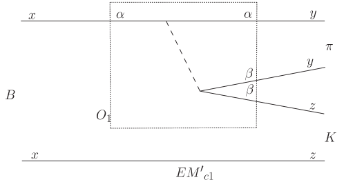
Class I: emission topologies: In these decays all the quarks in , apart from the quark, are contracted with quarks in the final state. The spectator quark has no contraction with any quarks in . These contractions therefore have an “inactive” spectator quark. There are two such contractions, and , which involve either an external or internal emission of final-state mesons. We therefore rename these with the ‘’ label:
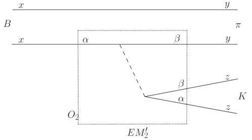
(9) The figures representing these contractions are given in Fig. 1.
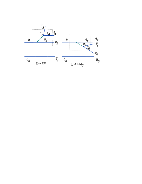
Figure 1: Emission topologies. Though not shown, the quark lines are dressed with gluons. Note that in factorization we have , where is the form factor and is the decay constant of . Hence, in this contraction is the emitted meson. Similarly, in factorization , and so here is the emitted meson. This contraction therefore corresponds to colour-suppressed emission, and hence the subscript is used in the label.
-
•
Class II: rescattering topologies: In these contractions the spectator quark does not contract with the quarks in and thus still remains “inactive.” However there is a contraction between the quarks in . There are two possible contractions, involving the pair (contractions and ) or the pair (contractions and ). For each pair the quarks in the final state can have contractions between quark pairs belonging to different mesons ( and ) or to the same meson ( and ). These latter contractions are expected to be small as they are Okubo-Zweig-Iizuka (OZI) suppressed.
A possible -type contraction arises from the rescattering contribution of the tree operators. Since such rescatterings are usually referred to as penguin contributions, we rename this contraction . Note that penguin operators can also produce this type of contractions. We rename the contraction as since a Fierz transformation of the operator makes the -type contraction look like an -type contraction. Finally, the OZI-suppressed contractions are renamed and :
(10) The figures representing these contractions are given in Fig. 2.
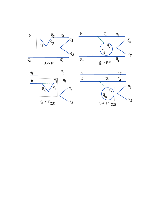
Figure 2: Rescattering topologies. Though not shown, the quark lines are dressed with gluons. In the QCDfac and pQCD approaches these rescattering contributions are perturbatively calculable. For a given operator such contributions are suppressed by at least relative to the contractions of the same operator belonging to Class I. For contractions involving charm quarks it is possible that rescattering may involve long-distance contributions that are not calculable perturbatively [7, 10]. To get an estimate of the size of the rescattering contributions from charm intermediate states through tree operators we can study charmless decays. Here there are no emission contractions for these operators; they can contribute only through rescattering contractions. Now, from experiments we know that these rescattering contractions are small and not of . If this were not the case, this would lead to too-large branching fractions for charmless transitions such as , etc. The rescattering from tree operators is then typically of the size of penguin amplitudes in charmless transitions. Using flavour symmetry, one can argue that rescattering through is also small.
Hence, for a given decay and a given operator, the emission contractions of class I, which do not suffer any colour suppression, are generally larger than the rescattering contractions generated by the same operator. To take a specific final state as an example, we expect the colour-allowed decay to get its dominant contribution from emission topologies. Such arguments can also be applied to NP operators and have been used to argue for small NP strong phases from rescattering contractions [9].
As noted above, the OZI-suppressed contractions are expected to be small. In fact, the -type contraction can contribute to the decay with a weak phase different from that of the dominant contribution through -quark rescattering. If such contributions were significant, the result would affect the measurement using this mode. The fact that the measurement [11] does appear to agree with predictions strengthens the claim that the OZI rescattering contributions are small.
-
•
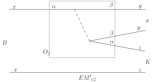
Class III: annihilation/exchange topologies: We identify the annihilation and exchange topologies with the and contractions, respectively. and involve contractions between quarks in the same mesons, and are therefore OZI-suppressed. We therefore rename the annihilation contractions as and , and the exchange contractions as and :
(11) These are shown in Fig. 3.
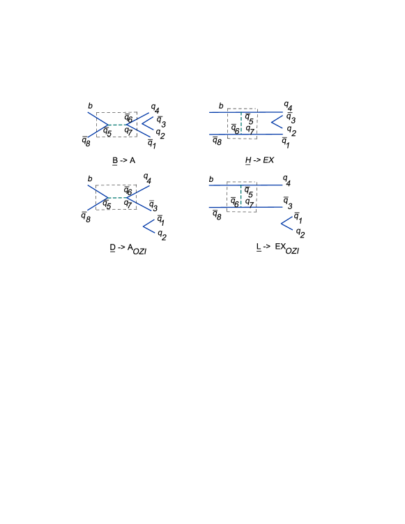
Figure 3: Annihilation/exchange topologies. Though not shown, the quark lines are dressed with gluons. This class of contractions is suppressed by . Whether such contributions are sufficiently small is a matter of debate which will ultimately be settled by observing (or not) decays such as or , which can only proceed through annihilation and exchange diagrams.
The OZI-suppressed contractions in this class are again expected to be small. Their size can be obtained from the measurement of decays such as [12] which can go through such OZI-suppressed contractions.
-
•
Class IV: topologies with annihilation/exchange rescattering: This class includes contractions that have annihilation and exchange in combination with rescattering. These include , , and . The contraction can be renamed for it is a “penguin-annihilation” contraction. Similarly, is a “penguin-exchange” contraction: . Note that and are OZI-suppressed while the contractions and suffer an additional OZI suppression; we rename them as and (Fig. 4):
(12) 
Figure 4: Topologies with annihilation/exchange rescattering. Though not shown, the quark lines are dressed with gluons. The contractions in this class are expected to be tiny as they are both -suppressed and OZI suppressed.
To summarize: there are 14 independent contractions. These can be
separated into four classes: ,
, ,
. In what follows, we will
almost always express amplitudes in terms of these contractions.
However, we will occasionally write amplitudes in terms of the 24
contractions – [Eq. (7)].
When we do this, we will be sure to give a warning of this fact. Thus,
unless there is an explicit statement to the contrary, the reader can
assume that all amplitudes are given in terms of the contractions
, , etc.
Buras-Silvestrini (BS) also have 14 topologies, described by rather complicated, nonstandard figures. They label these as DE (Disconnected Emission), CE (Connected Emission), DA (Disconnected Annihilation), CA (Connected Annihilation), DEA (Disconnected Emission-Annihilation), CEA (Connected Emission-Annihilation), DP (Disconnected Penguin), CP (Connected Penguin), DPE (Disconnected Penguin-Emission), CPE (Connected Penguin-Emission), DPA (Disconnected Penguin-Annihilation), CPA (Connected Penguin-Annihilation), (Disconnected Double-Penguin-Annihilation), (Connected Double-Penguin-Annihilation). Their eight OZI-suppressed topologies are DEA, CEA, DPE, CPE, DPA, CPA, , . As such, the starting point of our method is very similar to theirs. However, what they do is rather different from what we do in this paper.
BS’s main aim is to produce a manifestly scheme- and scale-independent formalism for hadronic decays. In the subsequent sections we show that this method reproduces results which have been obtained using other techniques. In particular, the results of diagrams, GPY, etc. can be simply expressed in terms of contractions.
BS stress the need to include the “small” OZI-suppressed contractions in order to obtain scheme- and scale-independent results. We agree with this observation, in principle. However, the BS paper was written before the observation that certain contractions are suppressed by factors of . Thus, in practice, these contributions are indeed small, and it is reasonable to neglect them when computing the amplitudes for hadronic decays. Including the small contractions makes the expressions for the amplitudes unnecessarily complicated.
2.2 Decays
In this subsection, we show how to compute the possible contractions for a given decay. We do so by considering the four decays: , , , .
We begin with . The operator that generates tree amplitudes involves and . Then
| (13) | |||||
where
| (14) |
For :
| (15) | |||||
In the above, we have expressed in the amplitude in terms of the contractions - of Eq. (7). Here and below, the primes on the contractions indicate a transition.
Now, final-state symmetry indicates that and . Using this, and changing the notation to that used in the four contraction classes, we then obtain for (dropping the label):
| (16) |
(Here, and indicate penguin and annihilation contractions, respectively.) In the above we have shown how final-state symmetry is used to include the and contractions. From here on, final-state symmetry will be assumed and not shown explicitly.
For :
| (17) |
Only the contraction is allowed and we get
| (18) |
For and , only the colour structure is different, so that
| (19) |
giving
| (20) |
where a sum over is understood.
The tree pieces of the other three decays can be found in the same way. In all, we have
| (21) |
Note that the quadrilateral isospin relation for decays is respected:
| (22) |
We now turn to the EWP operators. We make the approximation of neglecting and , so that the EWP operators are purely and are given by and alone.
In these operators, one sums over the light quarks, multiplied by their charge. Below we consider (with , ). Below we will always assume isospin symmetry, so that the contractions of and quarks are equal. However, we do not assume flavour SU(3) symmetry here (under SU(3) the contractions of , and quarks are equal). Instead the / and contractions are labeled individually.
The EWP contractions for the four decays can be found in the same way as was done for the tree operators. We have
| (23) |
Here, a sum over is understood. Note the appearance of the terms and . We remind the reader that the tilde indicates that the final state is as opposed to . Thus, for decays, the EWP contractions involve final states of the form . (To be more precise, EWP contractions involve terms which are equivalent to contractions, as per the equivalence table following Eq. (8).)
In the above, -quark and -quark contractions are taken to be equal (isospin symmetry). The / contractions have no label, while the contractions of -quarks are labeled by an ‘’ superscript. Because the operators in the two sets of contractions are different, the quarks are in different positions, and the equivalences due to final-state symmetry do not apply here. On the other hand, in the SU(3) limit, -quark, -quark and -quark contractions are equal, and the effect of SU(3) symmetry will be explicitly worked out in Sec. 4. One sees that, once again, the isospin quadrilateral is respected above.
We note in passing that there are rescattering contractions involving the quark for the EWP penguin operators which are represented by and . However these contributions are expected to be tiny relative to the rescattering from the tree operators. This is unlike the case of rescattering contractions involving the quark where the EWP contractions are enhanced by CKM factors relative to the tree contractions, so that both contractions are of the same size.
Finally, we turn to the gluonic-penguin operators. Here no WC’s can be neglected, so that all operators - must be included (i.e. we take into account both and Dirac structures). We have
| (24) |
which respects the isospin quadrilateral relation. The sum is over , and the index ‘’ indicates the Dirac structure.
In the above, we have made no assumptions about colours. That is, the quarks can have any colour, representing the exchange of any number of gluons. Thus, the above equations hold to all orders in . (We will work order-by-order in Sec. 5.)
In this subsection, we have shown how to write the matrix elements for the four decays in terms of contractions. This can be done for any hadronic decay. (Indeed, this is essentially what BS have done.) One important point is that, while we have expressed matrix elements in terms of contractions, we have not evaluated these matrix elements. This requires an additional method, such as QCDfac or pQCD.
3 Connection to Diagrams
All decays receive contributions from the penguin diagram, . (As with contractions, a prime on a diagram indicates a transition.) This diagram actually contains three pieces, corresponding to the identity of the internal quark:
| (25) |
Below we use this form for . Note that the unitarity of the Cabibbo-Kobayashi-Maskawa (CKM) matrix has not been used. This is because the unitarity of the CKM matrix was not used in writing the effective Hamiltonian [Eq. (1)].
When writing the amplitudes in terms of diagrams, it is conventional to absorb all () factors into the diagrams themselves. We then have
| (26) | |||||
In Ref. [6] it was shown that there is an EWP diagram corresponding to each of the , , , , , diagrams. These are included above. The first, second and third terms in square brackets are proportional to , and , respectively.
In the previous section it was shown how to write the contributions from tree, EWP and gluonic-penguin operators in terms of contractions. Using the above expressions, we can now write diagrams in terms of contractions. The tree-operator contribution is given in Eq. (21). Comparing with the first and second terms in parentheses above, we obtain
| (27) |
where the sum over is still understood. This matching looks very natural. Graphically, an emission contraction really looks like a diagram, and similarly for the colour-suppressed emission contraction, , and (Fig. 1). and are both described by the same type of contraction (Fig. 2), which represents rescattering from the operators . Finally, the contraction can be identified with annihilation diagram (Fig. 3).
The contribution from EWP operators is given in Eq. (23). Comparing to the EWP terms above, we have
| (28) |
Finally, the gluonic-penguin contribution is given in Eq. (24). This implies
| (29) |
Now, we note that Eqs. (27), (28) and (29) above are missing some diagrams: , , and . In order to obtain these, we must use a different decay. Here we choose the three decays: , , (recall that isospin symmetry has been assumed, so that the placement of the final-state pions is unimportant).
We simply present the results here; they can be derived using the techniques described previously. The tree contractions are
| (30) |
The EWP contractions are
| (31) | |||||
The contractions from the gluonic-penguin operators are
| (32) | |||||
In the above, the absence of a prime on the contractions indicates a transition. Note that, in all cases, the triangle isospin relation for decays is respected:
| (33) |
In terms of diagrams, the amplitudes for the three decays are given by
Comparing the amplitudes in terms of contractions and diagrams, we see that the missing diagrams are given by
| (35) |
For diagrams which appear in both and decays, the expressions for the connection to contractions are the same as in Eqs. (27), (28) and (29), except that the prime is removed.
| Diagram | Contraction | Diagram | Contraction |
|---|---|---|---|
| Diagram | Contraction |
|---|---|
The connection between diagrams and contractions is summarized in Table 1. One sees that the expressions for and are quite different from those for and , respectively. This is because and are derived from contractions involving -, while and involve and .
Note that this connection involves only 8 of the 14 independent contractions: , , , , , , , . The six OZI-suppressed contractions , , , , , are not used. The reason is the following. Each of these six involves the contraction of and and/or and . This can only happen if the final state contains neutral particles of the form . In the decays we have considered, only obeys this criterion. However, since , and since we have assumed isospin symmetry, the six contractions vanish. It is only if we consider final states involving a () or () that these contractions will contribute.
4 Connection to GPY
In this section, we show that, using contractions, one can reproduce the main results of Ref. [6], by Gronau, Pirjol and Yan (GPY). GPY use a group-theoretical formalism to analyze decays. On the other hand, the analysis using contractions is more direct. Throughout Ref. [6], GPY neglect the Wilson coefficients (WC’s) and , so that the EWP operators are purely . In what follows, we will make the same approximation. GPY also assume flavour SU(3) symmetry. We will (eventually) do likewise, but we will show how this assumption is necessary in our approach.
The first result is the following. The WC’s obey to about 5%. In the limit in which this equality is exact, GPY note that the EWP amplitudes (, , , , , ) are proportional to the tree operators (, , , , , ).
To see how these relations emerge in our formalism, we first concentrate on the diagrams and in decays. From Table 1, we see that these are proportional to and , respectively. These imply that the final states and , respectively, are produced. Now, we note that for only the up-quark piece of the electroweak operators contribute – this is denoted with an index . That is, involves only (as usual, the colour and Dirac indices have been suppressed). However, in the SU(3) limit, -quark contractions are equal to -quark contractions. Thus, . Equivalently, , so that the final states and are the same. Thus, . Things are similar for and , so that . We therefore see that
| (36) |
while
| (37) |
In the limit where , is proportional to .
The argument is much the same for and . In the SU(3) limit, we have and . Thus
| (38) |
and
| (39) |
As above, is proportional to in the limit where .
Things are simpler for the other four EWP diagrams , , , and . In the SU(3) limit, , so that is just proportional to (). Similarly, in the SU(3) limit, and is proportional to . Thus, all four EWP diagrams involve the same contractions as the corresponding tree diagrams , , and . For and we can therefore write
| (40) |
and
| (41) |
In the limit where , is proportional to . The argument is identical for the other three EWP diagrams , , and the tree diagrams , , .
We therefore see that the proportionality constant between the EWP and corresponding tree diagrams is , which agrees with GPY. In particular, we have
| (42) |
The second result is two relations between EWP and tree diagrams:
| (43) |
where . All the diagrams in the above relations are for decays, with the exception of , which is for . However, since flavour SU(3) has been assumed, and diagrams are equal.
In order to reproduce these relations, we make the following observation. In the limit of neglecting and , both EWP and tree operators are . In this case, it is possible to do a Fierz transformation to exchange the position of and without changing the Dirac structure of the operators. This results in and . If we also take the SU(3) limit, in which case one can switch and quarks, we have and . Given the equivalence of different operators, this implies that certain contractions are pairwise the same (within each of the four contraction classes):
| (44) |
Consider now the first relation. The left-hand side of the equality is
| (45) | |||||
The right-hand side is
| (46) | |||||
We therefore reproduce the first GPY EWP-tree relation using contractions.
We now turn to the second relation of GPY. The left-hand side of the equality is
| (47) | |||||
and the right-hand side of the equality is
| (48) | |||||
This proves the second EWP-tree GPY relation in .
We have therefore shown explicitly that, using contractions, we reproduce the main results of GPY [6] for decays.
It is worth making one final remark here. We have mentioned in Sec. 2.1 that the contractions and are higher order in . If these contributions are indeed small, then the second GPY relation can be separated into two relations, one leading order (LO), the other next-to-leading order (NLO). These contain the large and small contributions, respectively. We have
| (49) | |||||
Of course, each of these relations is individually satisfied.
5 Connection to QCDfac and pQCD
All the results in the previous sections hold to all orders in . As mentioned earlier, in our general approach, we are interested only in the possible ways in which the final-state quarks, which evolve into the final-state mesons, can be produced in decays through the effective Hamiltonian. That is, we do not attempt to calculate the strong interactions of the final-state quarks through the exchange of gluons and their ultimate hadronization into the final-state mesons. However, it is also possible to work order-by-order in by including the gluons explicitly. This is useful as it allows us to make a connection with QCDfac and pQCD, both of which work order-by-order. They do this because in their frameworks the nonleptonic amplitudes are expanded in powers of () for gluon exchanges involving the spectator quark, or for the remaining gluon exchanges.
The first calculation involves gluon exchanges only between quarks that belong to the same meson. In our approach, such gluon-exchange effects are taken into account automatically, and so we call this the (“zero-order”) calculation. This is in fact just the factorization assumption in calculating nonleptonic amplitudes.
The exchanged gluon between the quarks in a meson can be soft and hence these contributions are not perturbatively calculable. In the pQCD approach, the soft gluon-exchange contributions involving the soft spectator quark in the meson are argued to be highly suppressed. Thus, the soft spectator quark has to be boosted up in energy through gluon exchange in order to end up in the final-state light meson with energy . Since the gluon is relatively hard such contributions are calculable perturbatively in pQCD. However, it is not entirely clear that soft-gluon exchanges involving the spectator quark can be neglected, and in the QCDfac approach the soft-gluon contributions are absorbed in physical form factors.
In the second step we consider gluons exchanged between quarks belonging to different mesons []. In our approach we do not calculate the amplitudes explicitly. Instead, we work out the general structure of the contractions when one-gluon exchanges are included among the quarks that emerge from the decay through the weak effective Hamiltonian.
In the pQCD approach it is argued that such corrections are calculable perturbatively, while in the QCDfac approach the gluon exchanges involving the spectator quark are sensitive to long-distance physics. Thus, their effects, like the form factors, are represented by additional unknown hadronic quantities that may be obtained from a fit to data.
5.1 Order zero
In this section we will consider the zero-order calculation. From here on, we concentrate only on , , and in decays. In this case, with no gluons between quarks of different mesons, it is possible to take colours into account simply by counting them. For example, for we have
| (50) | |||||
In the above, the subscripts , , , and are colour indices. Since gluon exchanges among quarks belonging to different mesons are neglected, the contractions are simply proportional to delta functions in the colours:
| (51) | |||||
where the bar on is added to stress the fact that colour effects are extracted. The idea is the following: a priori the matrix elements and are different. But since the difference between and is only their colour structure, once we have taken this into account by explicitly adding the effect of colour, the remaining matrix elements are identical. Doing this for , , and , it is easy to derive the following relations
| (52) |
With SU(3), and taking into account Fierz transformations, we have . Then we obtain the two EWP-tree results of Eq. (42) (which hold to all-orders), and a third relation:
| (53) |
The numerical value of this ratio is obtained as follows. At leading order the WC’s take the values and (these values are taken from the last paper in Ref. [3]). Thus, taking , there is some cancellation between the factors in the numerator of Eq. (53). Now, the WC’s are calculated using a renormalization point of . However, in fact we do not know the precise value of – all we know is that it is . Allowing the values of the WC’s to vary leads to an uncertainty on the above ratio. The central value uses the above values for and , but the (estimated) error corresponds to allowing to vary. The bottom line is that the precise value of the ratio is uncertain. Still, although this ratio can be zero in the case of complete cancellation, there is an upper limit of approximately . We note in passing that the naive estimates of colour suppression are supported by the WC calculations.
Above, we have concentrated on , , and in decays. However, one can perform the above procedure for other contractions/diagrams. If one does so for the annihilation and exchange diagrams and , one finds the following interesting relation. At , the matrix elements are equal, so that
| (54) |
We therefore see that, at leading order, the diagram is expected to be much larger than . BS found a similar result, but in the large limit.
5.2 Corrections with 1 gluon
We now turn to the QCD corrections. We introduce a single gluon between all pairs of quarks in each diagram/contraction. We illustrate this procedure by considering the -type contraction for tree operators in (Fig. 5). There are ten possibilities for the gluon, shown in Fig. 6. Note that these include a possible gluon exchange between the quarks within the same meson – we will be able to absorb these corrections into the order-zero result.


We introduce the following notation: is the QCD correction () to the -type contraction (, ,…, ) of . is the same, except that the colours have been explicitly extracted: ).
The idea is the same as for the effects: the only difference between and is the colour structure. For example, and differ only in their colour structure, and so their matrix elements are equal once the colour effects have been extracted. The problem is more complicated here because there are several QCD corrections, e.g. we cannot relate to . Thus, the overall matrix elements are not equal unless all contributions appear in the same linear combination. We will see this explicitly below. Note also that matrix elements are still not evaluated.
We begin by computing the colour factor for
| (55) | |||||
Then vanishes by colour arguments. For ,
| (56) | |||||
The total contribution of the correction 1 to the contraction is then
| (57) |
A similar calculation has been performed for the remaining nine QCD corrections of the contraction , with the following result:
| (58) |
Because the coefficients of the two terms are not the same, the overall matrix element of is not the same as that of .
We can apply this to the diagram in decays. Let where is the piece without gluons [)] and is the piece with one-gluon corrections [)]. We have
| (59) |
However, an examination of Fig. 6 reveals that the corrections all correspond to gluon exchange between quarks within the same meson. As such, these corrections can be absorbed in the result. We will therefore rewrite Eq. 59 as as
| (60) |
This procedure can also be carried out for the contraction. Fig. 7 shows the -type contraction for colour-suppressed tree operators in . As before, we consider a single gluon exchange between all pairs of quarks. There are ten placements for these gluons, shown in Fig. 8.

Taking all one-gluon QCD corrections into account, we find
| (61) |
Thus, as for the contraction, the overall matrix element of is not the same as that of .
We now apply this to the diagram in decays: as with we define , with
| (62) |
However, like the contribution, the corrections can all be absorbed in the result. We therefore rewrite
| (63) |
Comparing the above expression to that of the diagram, we have in the SU(3) limit, leading to the observation that, at , the ratio is independent of matrix elements [Eq. (53)]. However, if we combine the and results, the ratio is not independent of matrix elements:
| (64) |
Note that the corrections to and are proportional to and , respectively. Since is quite a bit larger than , we therefore expect that the first-order correction to the ratio is also large. However, to obtain the exact value of beyond leading order, one needs to use a method to estimate the matrix elements. This establishes the connection between contractions and QCDfac/pQCD.
6 Is there a puzzle?
The amplitudes for the four decays are given in terms of diagrams in Eq. (3). Many of these diagrams are expected to be negligible (, , ) [2]. Retaining only those which are expected to be sizeable, we have
| (65) |
In the above, , , and we have explicitly written the relative weak phase (the phase information in the CKM quark mixing matrix is conventionally parametrized in terms of the unitarity triangle, in which the interior (CP-violating) angles are known as , and [13]).
The diagrams and are not independent – as has been shown, they are related to and . If we do not make the approximation that , we have
| (66) |
where
| (67) |
(If is assumed, the ratios of Eq. (42) are reproduced.)
The fact that can be expressed in terms of and was used in Ref. [14] to extract these CP phases from decays. However, and can also be obtained independently: can be taken from the measurement of mixing-induced CP violation in : [11], while can be found via a fit to independent measurements: [15]. In the fits which follow, we include these independent determinations of the weak phases.
Given that and can be related to and , the amplitudes in fact depend on only seven unknown theoretical parameters: the four magnitudes , , and , and their three relative strong phases. However, there are nine measurements: the branching ratios for the four decays, the four direct CP asymmetries , and the mixing-induced CP asymmetry in . The latest data is shown in Table 2.
| Mode | |||
|---|---|---|---|
It is therefore possible to perform a fit. We find a good fit: [16]. However, the fit also gives , whose central value is far larger than that given by the result [Eq. (53)]. This is the puzzle: present data seem to be inconsistent with naive SM predictions. (Above, we used the ratio to illustrate this point, but other quantities can be used as well.) Many analyses have found this result [17]. Note that, at present, the experimental errors are still quite large (and the theoretical errors, such as SU(3) breaking, have not been included), so that the effect of the puzzle is not yet statistically significant. As such, it can be said to offer only a hint of a discrepancy.
The purpose of this section is to critically re-examine the question of whether there is a puzzle. Assuming that the theoretical uncertainties are under control, and that the effect is not a statistical fluctuation – and these assumptions may well be wrong – the relevant question is: is it possible that ?
We begin with the expression for , Eq. (64):
| (68) |
The important question is, to what extent does the lowest-order (naive factorization) result for [Eq. (53)] represent the true SM value for this ratio? Note that if is included in the fit as a constraint, we obtain a very poor fit: , which corresponds to a deviation from expectations of [16]. Note also that our fit includes , and hence a large value of cannot lead to a good fit to the data (this is somewhat contrary to Ref. [18]).
In QCDfac the value of at may be raised to about 2-3 times the lowest-order result [19] and thus falls far short of the value required to fit the data. The fact that the first-order correction is quite large follows from the observation that and get corrections proportional to and , respectively [Eq. (64)], but is about 5-6 times larger than . Within pQCD, one also finds that the value of may be raised to 2-3 times the lowest-order result including NLO corrections [20]. Note that although the authors of Ref. [20] give results that are consistent with the central values of the direct CP asymmetries in the system, they cannot explain the central value of the indirect CP asymmetry in . On the other hand, our fit takes into account all data, including the indirect CP asymmetery in . One therefore has to be careful about the claim in Ref [20] that the puzzle is resolved within pQCD.
Although we do not have an all-orders result for to compare with the fit, we can still make several observations. It is true that higher-order effects, such as those from additional gluons, will affect the lowest-order result for and change its value. However, in order to produce a value that agrees with the fit, this value must change by a factor of 10! There are then two possibilities. One is that the true value of is large, which means that the corrections are very important. In this case, there is no puzzle. However, both methods of calculating matrix elements (QCDfac and pQCD) have argued for a reasonably small value of the strong coupling at the scale . Thus, the corrections are increasingly small. This in turn leads to a perturbative expansion for nonleptonic decays. Now, if there is really no puzzle, this means that the corrections are large, which sheds much doubt on the results of both QCDfac and pQCD. The other possibility is that the corrections are small and the true value of is similar to the result. In our opinion, this situation is more likely: we have small corrections, so that the lowest-order result for [Eq. (53)] is approximately correct, the results of QCDfac and pQCD are believable, and there is a puzzle.
7 Conclusions
We have presented a general approach to hadronic decays. The starting point is the observation that, at the quark level, the decay ( are mesons) involves the matrix elements , where , , and is an operator of the effective Hamiltonian (Dirac and colour structures are omitted here). In order to determine all possible ways in which the final-state quarks can be produced, it is necessary to sum over all possible Wick contractions of the quarks for all operators. The amplitude for can then be expressed as a sum over these contractions. In this paper we have examined various properties of these contractions.
There are a total of 24 possible contractions. However, due to the fact that we can write the final state as or , not all contractions are independent. We have shown that there are in fact only 14 independent contractions. Buras and Silvestrini (BS) obtained these results some years ago [8]. However, our analysis goes beyond that of BS in several ways, described below.
We have separated the independent contractions into four classes. Using recent theoretical and experimental developments, we have shown that certain contractions are smaller than others, and can occasionally be neglected. This greatly simplifies the expressions for the amplitudes in terms of contractions.
It is also possible to write the -decay amplitudes in terms of diagrams [2]. However, the relation between diagrams and the effective Hamiltonian was not made clear, and there was some question about the rigourousness of the diagrammatic approach. We have shown that all diagrams can be simply expressed in terms of contractions, thereby demonstrating formally that the diagrammatic method is rigourous.
In the limit of neglecting the (small) Wilson coefficients and , and assuming flavour SU(3) symmetry, Neubert/Rosner and Gronau/Pirjol/Yan have shown that there are relations between the electroweak-penguin and tree diagrams. We show that these relations are reproduced using the contractions method.
All of the above results hold to all orders in . That is, the contractions method includes the exchange of any number of gluons between the quarks. However, we have shown that it is also possible to work order-by-order in by including the gluons explicitly. This is useful, as it allows one to make a connection between the approach of contractions and the matrix-element evaluation methods of QCD factorization (QCDfac) and perturbative QCD (pQCD). If one works to leading order [], we have shown that one finds that in the SU(3) limit the ratio is independent of matrix elements ( and are, respectively, the colour-allowed and colour-suppressed tree diagrams in decays). In addition, this ratio is found the be rather small: . If one adds a single gluon [], this value changes, but one needs to evaluate matrix elements to determine its value.
Finally, we re-examine the question of whether there is a “ puzzle.” If one considers all data, a good fit is obtained, but is required. This central value is far larger than the result. Leaving aside the possibility of a statistical fluctuation, which might indeed be the true explanation, the question of whether or not there is a puzzle comes down to the question of whether or not additional gluons can change from 0.17 (the result) to 1.7. The higher-order effects have been evaluated in QCDfac and pQCD, and both methods find that is changed by at most 2-3 times the lowest-order result, instead of the required factor of 10. This is not surprising as both methods find that is relatively small at the scale . If were changed by a large amount, that would shed doubt on the smallness of , as well as all predictions of QCDfac and pQCD. We therefore conclude that it is likely that is relatively small (i.e. similar to the result), and that there really is a puzzle.
Acknowledgements:
We thank J. Charles, M. Gronau, J. Rosner and L. Silvestrini for helpful communications. M.I. thanks T. Mannel and T. Feldmann for useful physics discussions, and acknowledges the hospitality of LAPTH in Annecy, France and the Universität Siegen, Germany, where part of this work was done. This work is financially supported by NSERC of Canada.
References
- [1] See, for example, G. Buchalla, A. J. Buras and M. E. Lautenbacher, Rev. Mod. Phys. 68, 1125 (1996).
- [2] M. Gronau, O.F. Hernández, D. London, J.L. Rosner, Phys. Lett. B 333, 500 (1994), Phys. Rev. D 50, 4529 (1994), Phys. Rev. D 52, 6356 (1995). Phys. Rev. D 52, 6374 (1995).
- [3] M. Beneke, G. Buchalla, M. Neubert and C. T. Sachrajda, Phys. Rev. Lett. 83, 1914 (1999), Nucl. Phys. B 591, 313 (2000), Nucl. Phys. B 606, 245 (2001).
- [4] Y. Y. Keum, H. n. Li and A. I. Sanda, Phys. Lett. B 504, 6 (2001), Phys. Rev. D 63, 054008 (2001)
- [5] M. Neubert and J. L. Rosner, Phys. Lett. B 441, 403 (1998), Phys. Rev. Lett. 81, 5076 (1998).
- [6] M. Gronau, D. Pirjol and T. M. Yan, Phys. Rev. D 60, 034021 (1999) [Erratum-ibid. D 69, 119901 (2004)].
- [7] C.W. Bauer, D. Pirjol, I.Z. Rothstein, and I.W. Stewart, Phys. Rev. D 70, 054015 (2004); C.W. Bauer, I.Z. Rothstein, and I.W. Stewart, hep-ph/0510241.
- [8] A. J. Buras and L. Silvestrini, Nucl. Phys. B 569, 3 (2000).
- [9] A. Datta and D. London, Phys. Lett. B 595, 453 (2004); A. Datta, M. Imbeault, D. London, V. Page, N. Sinha and R. Sinha, Phys. Rev. D 71, 096002 (2005).
- [10] M. Ciuchini, E. Franco, G. Martinelli and L. Silvestrini, Nucl. Phys. B 501, 271 (1997); M. Ciuchini, E. Franco, G. Martinelli, M. Pierini and L. Silvestrini, Phys. Lett. B 515, 33 (2001).
- [11] B. Aubert et al. [BABAR Collaboration], Phys. Rev. Lett. 94, 161803 (2005); K. Abe et al. [Belle Collaboration], arXiv:hep-ex/0507037.
- [12] A. Datta, H. J. Lipkin and P. J. O’Donnell, Phys. Lett. B 529, 93 (2002).
- [13] Particle Data Group Collaboration, S. Eidelman et al., Phys. Lett. B 592 (2004) 1.
- [14] M. Imbeault, A. L. Lemerle, V. Page and D. London, Phys. Rev. Lett. 92, 081801 (2004).
-
[15]
The CKMfitter group, http://www.slac.stanford.edu
/xorg/ckmfitter/ckm_results_summerEPS2005.html - [16] We thank S. Baek for the numerical results of this fit.
- [17] A. J. Buras, R. Fleischer, S. Recksiegel and F. Schwab, Phys. Rev. Lett. 92, 101804 (2004), Nucl. Phys. B 697, 133 (2004), Acta Phys. Polon. B 36, 2015 (2005), arXiv:hep-ph/0411373; C. W. Chiang, M. Gronau, J. L. Rosner and D. A. Suprun, Phys. Rev. D 70, 034020 (2004); CKMfitter Group, J. Charles et al., Eur. Phys. J. C 41, 1 (2005); S. Mishima and T. Yoshikawa, Phys. Rev. D 70, 094024 (2004); Y. L. Wu and Y. F. Zhou, Phys. Rev. D 71, 021701 (2005); Y. Y. Charng and H. n. Li, hep-ph/0410005; X. G. He and B. H. J. McKellar, hep-ph/0410098; H. Y. Cheng, C. K. Chua and A. Soni, Phys. Rev. D 71, 014030 (2005); S. Baek, P. Hamel, D. London, A. Datta and D. A. Suprun, Phys. Rev. D 71, 057502 (2005).
- [18] Y. Grossman, A. Hocker, Z. Ligeti and D. Pirjol, Phys. Rev. D 72, 094033 (2005).
- [19] M. Beneke and D. Yang, Nucl. Phys. B736, 34 (2006); M. Beneke and M. Neubert, Nucl. Phys. B 675, 333 (2003).
- [20] H. n. Li, S. Mishima and A. I. Sanda, Phys. Rev. D 72, 114005 (2005).