Determination of Spin and CP of the Higgs Boson from WBF

Abstract:

We explore the possibilities to determine the spin/CP properties of the Higgs boson at the LHC. To cover the mass region below the ZZ threshold we make use of the properties of the production in Weak Boson Fusion (WBF) and the decay chain H $\rightarrow$ W⁺W^- $\rightarrow$ $\ell^{+}\nu\ell^{-}\nu$. In particular, we study the angular correlations of the forward jets and the distribution of the invariant mass of the lepton pair for different hypothetical Higgs like particles.

1 Introduction

The Standard Model (SM) is well established and in agreement with all present collider data. The only part of the model, not explored so far, is the Higgs sector. Because this sector plays a distinguished role in the theory, being responsible for the masses and mixings of all particles, the search for the Higgs boson is one of the highest priorities at the LHC. Within the Standard Model all properties of the Higgs boson are fixed when its mass is known. From indirect limits the Higgs boson is expected to have a mass in the range 114.4 GeV $<m_{H}<$ 246 GeV (95% C.L.) [1]. When the Higgs mass is above the $Z$ pair threshold, it decays with a large branching fraction into $Z$ bosons, that can be discovered in the “golden” $\ell^{+}\ell^{+}\ell^{-}\ell^{-}$ decay mode. As long as $m_{H}\gtrsim$ 130 GeV the decay into four leptons can still be used. Within the region 155 GeV $<m_{H}<$ 170 GeV the $ZZ^{*}$ branching fraction goes through a minimum, while the $WW^{*}$ decay mode opens up. In this mass range the $gg\to H\to WW\to\ell\nu\ \ell\nu$ [2] and the recently established vector boson fusion mode $qq\to qqH\to qqWW\to qq\ \ell\nu\ \ell\nu$ [4, 5, 6] have the largest discovery potential.

In recent papers [8, 3] we discussed the possible determination of the spin/CP properties of the Higgs boson. To analyse these properties we introduced hypothetical couplings to the Z-bosons corresponding to a Higgs-like particle with non Standard Model spin and CP. To distinguish different spin/CP eigenstates we considered the decay chain $H\to ZZ\to\ell^{+}\ell^{-}\ell^{+}\ell^{-}$ and analysed the angular correlations between the leptons. In [8] we discuss pure spin/CP states up to spin 1, [3] also considers spin 2 particles performing a similar analysis. In addition we also consider mixed CP states for spin 0 particles in [7]. These analyses showed that the spin/CP properties can easily be determined for a Higgs mass above the threshold for Z pair production. Below the threshold it is more challenging to obtain a significant separation.

To cover this mass region we now investigate Higgs production via WBF and the subsequent decay chain $H\to WW\to\ell\nu\,\ell\nu$. Promising observables in this case are the angle between the two forward jets and the invariant mass of the charged leptons.

A similar analysis using only the angle between the tag jets has already been performed in [4]. They considered additional dimension six operators to couple a spin 0 Higgs boson to vector bosons including a CP odd and a CP even coupling not present in the Standard Model.

The NLO corrections to Higgs production via WBF are given in [9]. They do not significantly change the shape of the distributions and therefore we limit ourselves to the leading order approximation.

The paper is organized as follows. In chapter 2 we briefly review the model used for the non Standard Model couplings, in chapter 3 we discuss the angular distributions of the tag jets and the invariant mass of the lepton pair and finally we conclude.

2 Model

We use the same parametrisation as introduced in [8] and only repeat it here for completeness.

The most general coupling of a (pseudo) scalar Higgs boson with mass $M_{h}$ to two on-shell vector bosons is of the following form:

$${\cal L}_{scalar}=\mathbf{X}\delta_{\mu\nu}+\mathbf{Y}k_{\mu}k_{\nu}/M_{h}^{2}+i\mathbf{P}\epsilon_{\mu\nu p_{Z}q_{Z}}/M_{h}^{2}.$$ (1)

Here the momentum of the first boson is $p_{Z}^{\mu}$, that of the second boson is $q_{Z}^{\nu}$. The momentum of the Higgs boson is $k$ and $\epsilon_{\mu\nu\rho\sigma}$ is the total antisymmetric tensor with $\epsilon_{1234}=i$. Within the Standard Model one has $\mathbf{X}=1$, $\mathbf{Y}=\mathbf{P}=0$. For a pure pseudoscalar particle one has $\mathbf{P}\not=0,\mathbf{X}=\mathbf{Y}=0$. If both $\mathbf{P}$ and one of the other interactions are present, one cannot assign a definite parity to the Higgs boson.

A similar formula for a (pseudo) vector with momentum $k_{\rho}$ reads:

$${\cal L}_{vector}=\mathbf{X}(\delta_{\rho\mu}p_{Z}^{\nu}+\delta_{\rho\nu}q_{Z}^{\mu})+\mathbf{P}(i\epsilon_{\mu\nu\rho p_{Z}}-i\epsilon_{\mu\nu\rho q_{Z}}).$$ (2)

It is to be noted that the coupling to the vector field actually contains only two parameters and is therefore simpler than to the scalar.

Using the generalised couplings given above we calculated the matrix elements for $qQ\to q^{\prime}Q^{\prime}H$ where the primed and unprimed quarks belong to the same $SU(2)$ doublet. In combination with the matrix elements for $H\to WW\to\ell\nu\,\ell\nu$ given in [8] the full matrix element for $qQ\to q^{\prime}Q^{\prime}\ell\nu\,\ell\nu$ can be obtained. Using this result an event generator was written to study the effects of the various cuts. The QCD background has been simulated using Pythia[12] while we used Madgraph/Madevent[11] for the electroweak background.

3 Reconstruction and analysis

The ATLAS collaboration has demonstrated, that the H $\rightarrow$ WW $\rightarrow\ell\nu\,\ell\nu$ signal can be reconstructed very well above a very small background using only 30 fb^-1 [5]. This makes this channel a very promising candidate for the discovery of the Higgs boson. We will use the cuts described there and normalise our samples to the number of signal and background events found in that very detailed study. We will discuss the effect of some of the cuts on the results we get, and vary them to show how a bias in the measured quantities can be reduced in exchange for a higher background level.

We will give a short summary of the main features of the signal selection, but not repeat the cuts in all detail (please refer to [5]). We require two leptons with high transverse momenta (P${}_{T}^{1}>$ 20 GeV and P${}_{T}^{2}>$15 GeV) to ensure that the events can be reliably triggered on. The main part of the reconstruction consists of the selection of two jets in the forward direction (the tag jets) with a large separation in rapidity, combined with a veto on hard jets in the rapidity region between the tag jets. This exploits the fact that the signal process lacks colour flow in the t-channel, unlike the most prominent background - namely $t\bar{t}$ production. A moderate cut on the dijet mass is imposed. The jets are used to balance the momentum of the decay products of the Higgs, so that a cut on the transverse momentum of this system consisting of the two jet, the leptons and the missing transverse momentum can be applied. We will use the angle between the two jets as one of the variables, that allows us to determine if the spin/CP state of the particle found is consistent with that of the SM Higgs boson.

The other major aspect of the ATLAS analysis deals with correlations of the decay leptons. Based on a spin/CP hypothesis of 0⁺ for the Higgs boson, the decay products will have certain angular correlations, that differ from those of the background processes. Cuts on the angle $\phi$ between the two leptons in the transverse plane, on the separation in rapidity $\eta$ and $\phi$, the cosine of the polar opening angle and the mass of the di-lepton system are applied in order to maximise the signal to background ratio. Obviously, these cuts interfere with the determination of spin and CP. We will study the effect of these cuts on the significance of the spin and CP measurement.

The potential background from Z$\rightarrow\tau\tau$ can be suppressed by trying to reconstruct the $\tau$ leptons in a collinear approximation using the missing transverse momentum, and imposing a lower limit on the transverse mass of the di-lepton and neutrino system. While the Z$\rightarrow\tau\tau$ background can be effectively suppressed by this, the cuts used have a negligible effect on the quantities used in this analysis.
For the further discussion we define the following subsets of cuts:
The “tagging cuts” are those, that define the tag jets and select the signal using these jets:

• Two leptons with transverse momenta $P_{T}>15$ GeV and one lepton with $P_{T}>20$ GeV and rapidity $|\eta|<2.5$

• Two jets with $P_{T}^{1}>40$ GeV and $P_{T}^{2}>20$ GeV with a separation in rapidity $\delta\eta>3.8$ and the two leptons lie within this gap.

• The dijet mass $M_{jj}>$ 550 GeV

The “lepton cuts” further suppress the background and can bias the spin/CP measurements:

• The angle between the two leptons in the transverse plane $\Delta\phi_{\ell\ell}\leq 1.05$

• Separation in the $\eta$-$\phi$-plane $\Delta R_{\ell\ell}\leq 1.8$

• Cosine of the polar opening angle $\cos\theta_{\ell\ell}\geq 0.2$

• Di-lepton mass $M_{\ell\ell}<$ 85 GeV

• Transverse momentum $P_{T}(\ell_{1,2})<$ 120 GeV

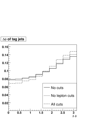
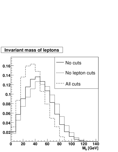
Figure 1: The effect of the cuts on the jet angle (left) and di-lepton mass (right) distributions of the SM Higgs assuming a Higgs mass of 150 GeV. The solid lines reflect the distribution at tree level without any cuts applied. The dashed line shows the distributions with only the tagging cuts applied and the dash-dotted one with all cuts.

3.1 Tag jet angle

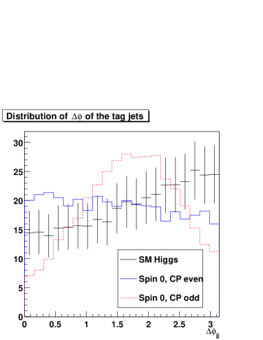
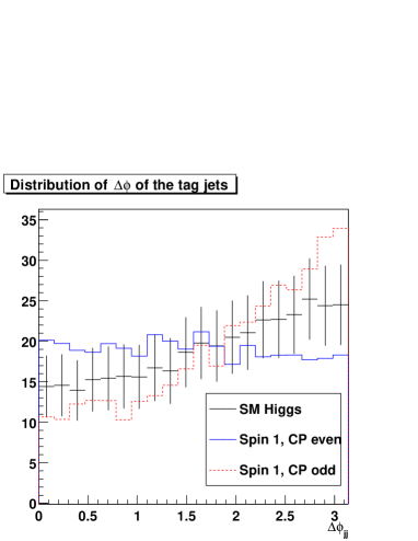
Figure 2: The distributions of the tag jet angle for the non SM couplings with a Higgs mass of 150 GeV. The points with error-bars show the SM distribution. The errorbars indicate the expected statistical error with an integrated luminosity of 30 fb^-1 neglecting the background contribution.

While the rapidity gap between the forward jets in WBF is due to lack of colour flow, the angle between the jets highly depends on the coupling structure of the Higgs to the vector bosons. This can be exploited to determine the structure of the coupling by comparing the measured distribution of the selected tag jets to the distributions expected for non SM couplings. Some of the cuts used to select the signal process have the potential to bias the distribution. A lower limit on the dijet mass should favour higher angles between the jets, and the cuts on the decay particles could have different effects. Figure 1 illustrates the effect of different sets of cuts on the tag jet angle for a Higgs boson mass of 150 GeV. The solid line shows the distribution on parton level with no cuts applied. When all but the lepton cuts are applied the distribution becomes slightly steeper (dashed) and when finally all cuts are applied (dash-dotted) it steepens even further. But overall the effects are rather small, and do not diminish the power of this variable to discriminate between different spin/CP states. Figure 2 shows the distribution of the tag jet angle for various spin/CP states and a Higgs mass of 150 GeV. The error-bars indicate the expected number of events for a SM Higgs and the expected statistical error when using the results of [5]. The dashed and solid lines show the expected distributions of the other spin 0 (left) and spin 1 (right) hypothesis. All histograms are normalised to the expected number of events in the SM as any significant deviation would rule out a SM Higgs directly. All non SM couplings show significant deviations from the SM case, especially the spin 0, CP odd case.

To evaluate the feasibility of the measurement, we use simulated samples of SM Higgs signal events and samples of background events, where the number of events in these samples is taken from [5]. We then compare the tag jet angle distribution of these samples with SM and non SM distributions derived from larger MC samples. All samples have passed the same complete list of cuts, and thus the potential bias introduced by those cuts is modeled correctly. We use a binned likelihood to evaluate how significant the deviation from the non SM models is. For large event numbers the ratio $2\mathrm{ln}(L_{SM}/L_{NSM})$ corresponds to the standard deviation of a $\chi^{2}$ test. In figure 3 we plot the mean likelihood ratio for a large number of MC experiments and the RMS of the distributions of the likelihood ratio.

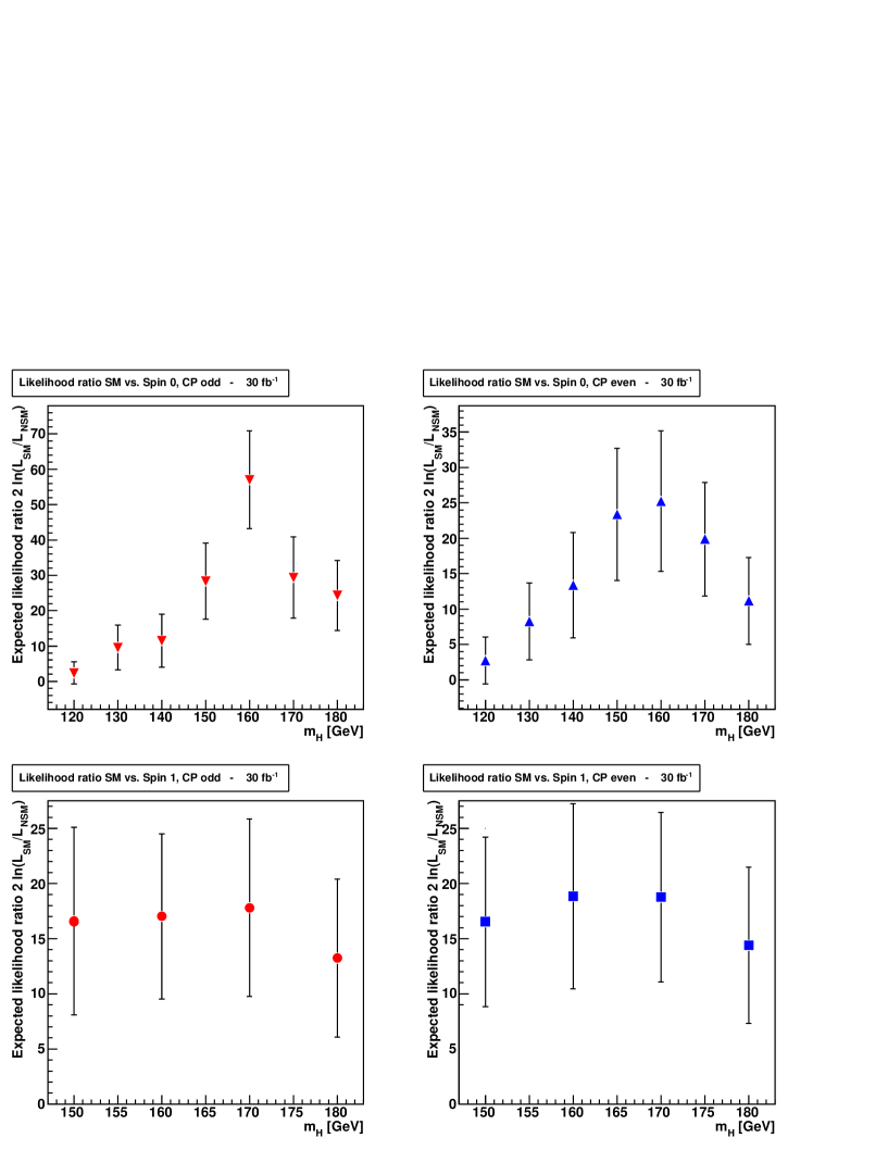
Figure 3: Exclusion significance from jet angles using 30 fb^-1. The points show the mean log likelihood ratio $2\mathrm{ln}(L_{SM}/L_{NSM})$. The error-bars reflect the RMS of the distribution of the likelihood ratio. 2/3 of a large number of experiments would yield a result within this range.

3.2 Di-lepton mass

It has been suggested [5] that the distribution of the angle between the leptons in the transverse plane could be used to verify the SM spin/CP hypothesis. Unfortunately, the SM and the non SM distributions all peak at small angles (see figure 4). Furthermore, the angle is obviously not Lorentz invariant, so that an initial state boost would change the distributions. Considering potential problems in modeling initial state radiation (ISR) at the LHC, we would forfeit the main advantage of using the very clean and well measurable leptonic decay products. We avoid such complications by using the invariant di-lepton mass which is correlated to the angular distributions, and peaks at different values for the various scenarios (figure 5). Probably the most straight forward variable to use is the mean value of the invariant mass distribution. Again, we will determine the feasibility using a number of MC samples and determine the mean and RMS of the distribution of the mean di-lepton mass.

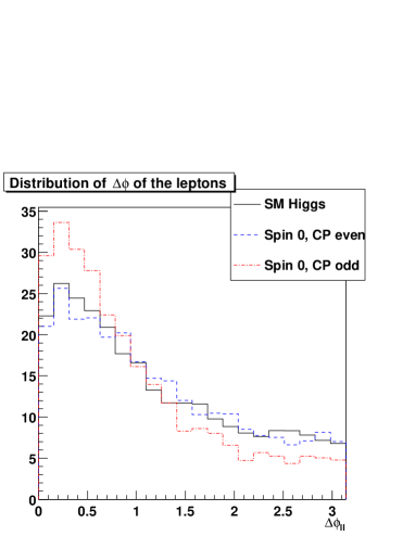
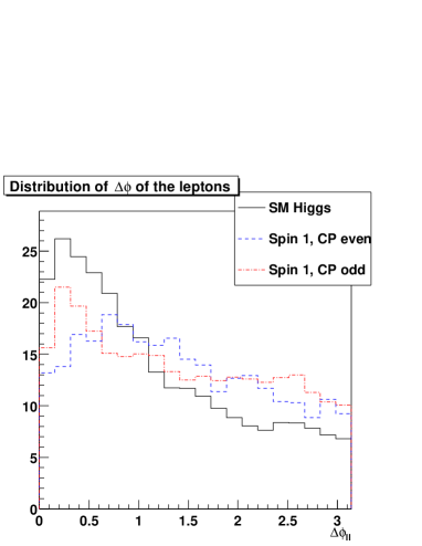
Figure 4: The distribution of the angle between the leptons in the transverse plane for the SM and non SM couplings and a Higgs mass of 150 GeV. All distributions peak around 0. ISR will have a direct effect on these distributions.

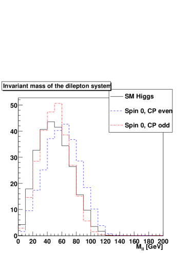
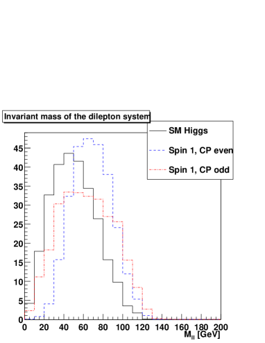
Figure 5: The distribution of the di-lepton mass for SM and non SM couplings and a Higgs mass of 150 GeV. The mass is highly correlated to the lepton angle but invariant, so that ISR will not affect the distribution.

The most problematic aspect of this analysis is the obvious bias introduced by the lepton cuts (see figure 1). Since larger angles are correlated with a larger invariant mass of the di-lepton system, the cuts on the angle in the transverse plane and the cut on the separation in the R-$\phi$-plane bias the distribution significantly and shift the mean towards smaller values for all couplings. The distinguishing power of this variable is thereby decreased.

We list the expected mean for the various couplings and different sets of cuts in table 1 for a Higgs mass of 160 GeV. For clarity we neglect any background for the numbers in this table. They would introduce varying offsets for the different sets of cuts. Of course, these effects are included when determining the exclusion significances, where they have a minor effect, as they mostly cancel out in the mean mass differences.

We define a set of relaxed lepton cuts as follows (numbers in brackets show the standard values as determined in [5]): The cut on the angle of the leptons in the transverse plane is changed to $\Delta\phi_{\ell\ell}\leq 1.9$ (was 1.05), the separation in the $\eta$-$\phi$-plane to $\Delta R_{\ell\ell}\leq 2.5$ (was 1.8), the cosine of the polar opening angle to $\cos\theta_{\ell\ell}\geq 0.0$ (was 0.2). The signal region is defined by the di-lepton mass $M_{\ell\ell}<$ 100 GeV (was 85 GeV) and the transverse mass $m_{\ell\ell\nu}<$180 GeV (was 175 GeV). The cut on the upper bound of the lepton $P_{T}$ remains unchanged. The more extreme case where the cuts on $\Delta\phi_{\ell\ell}$, $\Delta R_{\ell\ell}$ and $\cos\theta_{\ell\ell}$ are completely dropped and the signal region is widened even further to $M_{\ell\ell}<$ 120 GeV and $m_{\ell\ell\nu}<$ 200 GeV will be called “no lepton cuts”. Loosening the cuts on these variables obviously leeds to a rise in the expected background. In table 1 we list the increase of the background relative to the expected background given in [5]. As we do not use any detector simulation, we are not able to reproduce the absolute number of events expected, but the relative numbers given here are reliable, since they depend mostly on cuts on very well measured quantities related to the high $P_{T}$ leptons. The largest contribution to the background comes from top pair production and the electroweak WW processes. The QCD WW production is well enough suppressed by cuts on the tag jets, so that even with the rather high relative efficiency from the relaxed cuts it still doesn’t contribute much to the background. Taking all three backgrounds and their respective fractions of the total background (from [5]) into account we can estimate the increase of the background to be from 2.5 for the relaxed cuts to 4.5 with no lepton cuts. This and the rise in signal are compatible with what can be seen in the plots in [5].

	mean $M_{\ell\ell}$/GeV					relative efficiencies
cuts	SM	0+	0-	1+	1-	Signal	tt	WW(qcd)	WW(ew)
Standard	36.7	43.3	40.7	53.3	39.4	1	1	1	1
Relaxed	45.3	56.2	48.5	65.3	52.4	1.92	2.47	2.80	1.78
No lepton	50.2	62.2	50.7	70.2	63.9	2.90	4.48	6.76	3.80

Table 1: The effect of different sets of cuts on signal and background, and on the expected mean of the di-lepton mass for a Higgs boson of 160 GeV.

While the lepton cuts reduce the background, they also reduce the number of signal events and the differences in the di-lepton mass. We explore the effect of the three different cuts sets, taking into account the effects on the distributions and the change in number of signal and background events. We use samples with the expected number of signal and background events and calculate the mean of the di-lepton mass. Doing this for many samples, we then use the mean of those means as the expected value, and the RMS of the means as the expected error. In figure 6, we plot the difference between SM and non-SM values divided by the expected error. From these we can see, that the spin 1, CP even case can be ruled out using the di-lepton mass with any of the sets of cuts, while the Spin 1 CP odd case becomes too similar to the SM case, when applying any lepton cuts. However, it can be ruled out for some Higgs masses when the lepton cuts are completely dropped.

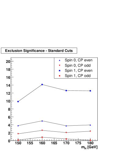
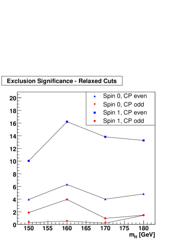
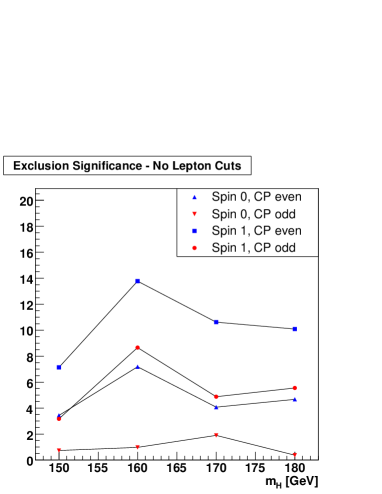
Figure 6: The expected exclusion significance of non SM couplings, using three different sets of cuts. The standard set of cuts as defined in [5] (upper left), the relaxed lepton cuts (upper right) and no lepton cuts (bottom).

4 Conclusions

We have implemented a matrix element generator capable of simulating the generation of Higgs bosons via WBF and its decay to W pairs with SM and non SM spin and CP quantum numbers (namely $0^{+},0^{-},1^{+},1^{-}$). We have demonstrated that the different couplings lead to distinct distributions of the opening angle of the tag jets and the invariant mass of the leptons from the leptonic decay of the W pairs. The latter distributions are very sensitive to the lepton cuts used to isolate the signal. This leads to the necessity of optimizing these cuts carefully when performing the measurement using real data, depending on the background level observed in the experiment. The tag jet distributions appear much more robust against the cuts. They provide very promising prospects to confirm the spin/CP state of an SM Higgs with a mass between 130 and 180 GeV using an integrated luminosity of 30fb^-1.

References

- [1] S. Eidelman et al. [Particle Data Group], Phys. Lett. B 592 (2004) 1.
- [2] M. Dittmar and H. K. Dreiner, Phys. Rev. D 55 (1997) 167 [arXiv:hep-ph/9608317].
- [3] S. Y. Choi, D. J. Miller, M. M. Muhlleitner and P. M. Zerwas, Phys. Lett. B 553 (2003) 61 [arXiv:hep-ph/0210077].
- [4] D. L. Rainwater and D. Zeppenfeld, Phys. Rev. D 60, 113004 (1999) [Erratum-ibid. D 61, 099901 (2000)] [arXiv:hep-ph/9906218].
- [5] S. Asai et al., Eur. Phys. J. C 32S2 (2004) 19 [arXiv:hep-ph/0402254].
- [6] S. Abdullin et al., CMS NOTE 2003/033.
- [7] C. P. Buszello, P. Marquard and J. J. van der Bij, arXiv:hep-ph/0406181.
- [8] C. P. Buszello, I. Fleck, P. Marquard and J. J. van der Bij, Eur. Phys. J. C 32 (2004) 209 [arXiv:hep-ph/0212396].
- [9] T. Figy, C. Oleari and D. Zeppenfeld, Phys. Rev. D 68 (2003) 073005 [arXiv:hep-ph/0306109].
- [10] V. Del Duca, W. Kilgore, C. Oleari, C. R. Schmidt and D. Zeppenfeld, Phys. Rev. D 67 (2003) 073003 [arXiv:hep-ph/0301013].
- [11] F. Maltoni and T. Stelzer, JHEP 0302 (2003) 027 [arXiv:hep-ph/0208156].
- [12] T. Sjostrand, L. Lonnblad, S. Mrenna and P. Skands, arXiv:hep-ph/0308153.