CALTECH MAP-319

CPT-P05-2006

FTUV/06-0319

IFIC/06-02

UWThPh-2005-19

Towards a consistent estimate of

the chiral low-energy constants

V. Cirigliano¹, G. Ecker², M. Eidemüller³,

R. Kaiser⁴, A. Pich³ and J. Portolés³

¹⁾ California Institute of Technology

Pasadena, California 91125, USA

²⁾ Institut für Theoretische Physik, Universität Wien

Boltzmanngasse 5, A-1090 Vienna, Austria

³⁾ Departament de Física Teòrica, IFIC, CSIC — Universitat de València

Edifici d’Instituts de Paterna, Apt. Correus 22085, E-46071 València, Spain

⁴⁾ Centre de Physique Théorique, CNRS-Luminy, Case 907,

F-13288 Marseille Cedex 9, France

Guided by the large-$N_{C}$ limit of QCD, we construct the most general chiral resonance Lagrangian that can generate chiral low-energy constants up to ${\cal O}(p^{6})$. By integrating out the resonance fields, the low-energy constants are parametrized in terms of resonance masses and couplings. Information on those couplings and on the low-energy constants can be extracted by analysing QCD Green functions of currents both for large and small momenta. The chiral resonance theory generates Green functions that interpolate between QCD and chiral perturbation theory. As specific examples we consider the $\langle VA\,P\rangle$ and $\langle S\,P\,P\rangle$ Green functions.

PACS : 11.15.Pg, 12.38.-t, 12.39.Fe
      Keywords : Chiral Lagrangians, $1/N_{C}$ expansion, QCD.

1 Introduction

Chiral perturbation theory [1, 2, 3] ($\chi$PT) is the effective theory of QCD at small external momenta. In the low-energy regime, the leading singularities of QCD Green functions of quark currents are generated by the octet of light pseudoscalar mesons ($\pi,K,\eta$), the explicit degrees of freedom in the effective theory. $\chi$PT is constructed by exploiting the chiral symmetry of QCD in the limit of massless light quarks (we consider here the three-flavour case with $m_{u}=m_{d}=m_{s}=0$), its spontaneous symmetry breaking according to the pattern $SU(3)_{L}\times SU(3)_{R}\rightarrow SU(3)_{V}$ and its explicit breaking due to nonvanishing quark masses.

The structure of the effective Lagrangian is determined by chiral symmetry and the discrete symmetries of QCD. It is organized as an expansion in derivatives of the Goldstone fields and in powers of the light quark masses ($m_{q}$). In the standard scenario the two expansions are related ($m_{q}\sim{\cal O}(M^{2})\sim{\cal O}(p^{2})$) and the mesonic effective chiral Lagrangian takes the form

$${\cal L}_{\rm eff}=\sum_{n\geq 1}\ {\cal L}_{2n}^{\rm\chi PT}\ ,\qquad\qquad\qquad{\cal L}_{2n}^{\rm\chi PT}\sim{\cal O}(p^{2n})\,.$$ (1.1)

The intrinsic scale $\Lambda_{\chi}$ of this expansion is set by the lightest mesonic non-Goldstone states ($\Lambda_{\chi}\sim M_{V}\sim 1$ GeV). The effective Lagrangian depends on a number of low-energy constants (LECs), which are not determined by symmetry considerations, encoding the underlying QCD dynamics. Applications of current interest require working to NNLO (${\cal O}(p^{6})$) [4]. Since ${\cal L}_{6}^{\rm\chi PT}$ involves 90 LECs for three light flavours [5, 6, 7], a theoretical assessment of the size of those couplings is mandatory for phenomenology.

Determining the LECs from QCD is a difficult nonperturbative problem. However, both empirical evidence and theoretical arguments suggest that the most important contributions to the LECs in the strong chiral Lagrangian come from physics at the scale $\Lambda_{\chi}$, i.e. the physics of low-lying resonances. In general, the LECs can be characterized as coefficients of the Taylor expansion of QCD correlators around zero momentum, once the non-expandable singularities due to Goldstone modes have been removed. If the appropriate correlators are order parameters of spontaneous chiral symmetry breaking (vanishing to all orders in QCD perturbation theory), they fall off at high momenta with an inverse power determined by the operator product expansion (OPE). Therefore, the LECs are expected to be sensitive to the intermediate-momentum region where the low-lying hadronic resonances turn the polynomial behaviour of the correlator into an inverse-power behaviour, as required by the QCD short-distance constraints.

The natural framework to incorporate systematically the above considerations is provided by the $1/N_{C}$ expansion of QCD [8, 9]. Earlier studies of resonance saturation for ${\cal O}(p^{4})$ couplings  [10, 11, 12] can be embedded in this framework [13, 14, 15]. A number of more recent works has already applied large-$N_{C}$ techniques to estimate subsets of the ${\cal O}(p^{6})$ LECs [16, 17, 18, 19, 20, 21]. A few studies at next-to-leading order in the $1/N_{C}$ expansion have also been performed [22]. In this work we aim to study systematically resonance contributions to the full ${\cal L}_{6}^{\rm\chi PT}$ to leading order in $1/N_{C}$. We first recall the salient features common to most procedures based on the $1/N_{C}$ expansion, describing along the way several approximations used in this work. We then comment on the specific aspects that characterize the interaction between Goldstone modes and resonance fields.

Matching at large $N_{C}$

In principle, the matching of QCD with $\chi$PT is straightforward in the $N_{C}\rightarrow\infty$ limit (QCD_∞). To leading order in the $1/N_{C}$ expansion, any correlator of quark bilinears $\langle J_{1}...J_{n}\rangle$ is given by a sum of tree-level diagrams involving interactions of an infinite tower of narrow meson states with appropriate quantum numbers . Hadron masses and couplings are adjusted so as to satisfy chiral Ward identities and to match the QCD asymptotic behaviour at large momenta. The Taylor expansion of the correlator around vanishing momenta, after removing the Goldstone poles, allows one to read off the corresponding chiral LECs.

In practice, since a solution to QCD_∞ is not available, one has to make a set of approximations in implementing the matching outlined above. The main approximations involve truncating the hadronic spectrum to a finite number of states and choosing the appropriate set of short-distance constraints to determine the hadronic parameters. In this work we truncate the spectrum to the lowest-lying resonance multiplets with given $J^{PC}$. We consider explicitly the channels V($1^{--}$), A ($1^{++}$), S ($0^{++}$), P($0^{-+}$). This choice has to be considered a working hypothesis that can be extended if needed. It is based on the observations that (i) the low-lying hadronic spectrum has the largest impact on the LECs; (ii) the QCD asymptotic behaviour sets in at energies $E\sim 1.5$ GeV (for correlators that are order parameters of spontaneous chiral symmetry breaking the fall-off is well reproduced by a few hadronic states [13]); (iii) retaining only lowest-lying states leads to a successful phenomenology for ${\cal O}(p^{4})$ couplings [10].

In this work we disregard the lightest P($0^{-+}$) singlet because the $\eta^{\prime}$ meson plays a special role in the large-$N_{C}$ counting [3, 23, 24]. The contributions of $\eta^{\prime}$ exchange to the LECs of ${\cal O}(p^{6})$ are worked out in an accompanying paper [25].

Concerning the short-distance constraints, the minimal requirement is that the Green functions obey the asymptotic behaviour dictated by QCD to leading power in the inverse large momenta. In addition, although not derived from first principles, it is heuristically inferred [26] and phenomenologically supported that form factors of QCD currents should vanish smoothly at large momenta. It should be kept in mind, however, that there are intrinsic limitations of the matching program when only a finite number of resonance multiplets are included (e.g., Refs. [19, 21]).

Lagrangian formulation

The matching strategy outlined above can be pursued within or without a Lagrangian description of the chiral invariant Goldstone-resonance interactions. One useful aspect of the Lagrangian formulation is that, within a given set of assumptions on the large-$N_{C}$ spectrum, it provides a common framework to study many observables or correlators at the same time as opposed to constructing different hadronic ansätze on a case-by-case basis. Another important feature of the Lagrangian approach is that the resonance fields can be integrated out at the level of the generating functional as opposed to expanding resonance propagators in individual Green functions. This allows one to obtain all resonance contributions to the ${\cal O}(p^{6})$ chiral LECs once and for all, even before specific values of the resonance couplings have been determined by the short-distance analysis.

In the strict large-$N_{C}$ limit the hadronic Lagrangian ${\cal L}_{\infty}$ has to be used at tree level only. Its couplings are determined in such a way that the corresponding Green functions reproduce the asymptotic behaviour of QCD_∞. Although the construction of ${\cal L}_{\infty}$ is a formidable task, progress can be made if one considers a limited set of hadronic states and if one focuses on the subset of ${\cal L}_{\infty}$ that, upon integrating out heavy fields at tree level, contributes to the chiral Lagrangian up to a given chiral order only. This limits both the number of resonance fields and the chiral order of the respective terms in the resonance Lagrangian. The first systematic studies in this direction go back to Refs. [10, 11] where the most general ${\cal L}_{\infty}$ contributing to ${\cal L}_{4}^{\rm\chi PT}$ was constructed and the equivalence of different representations for spin-one fields was demonstrated, once the Green functions generated by ${\cal L}_{\infty}$ are forced to satisfy the correct asymptotic behaviour dictated by QCD.

In this paper we perform the first steps towards a systematic study of resonance contributions to ${\cal L}_{6}^{\rm\chi PT}$ within the truncated large-$N_{C}$ matching described above. The program involves several tasks:

1. Construct the most general chiral invariant Lagrangian describing the interactions of Goldstone modes with V, A, S, P meson resonance fields that contributes to ${\cal L}_{6}^{\rm\chi PT}$ after integrating out the resonance fields. Apart from kinetic and mass terms for the resonance fields, it has the following structure:

   $${\cal L}_{\infty}\ ={\cal L}^{\rm GB}_{(2)+(4)+(6)}\ +\ {\cal L}^{R_{i}}_{(2)}+{\cal L}^{R_{i}}_{(4)}\ +\ {\cal L}^{R_{i}R_{j}}_{(2)}\ +\ {\cal L}^{R_{i}R_{j}R_{k}}_{(0)}\ ,$$ (1.2)

   where ${\cal L}^{\rm GB}_{(2)+(4)+(6)}={\cal L}_{(2)}^{\rm GB}+{\cal L}_{(4)}^{\rm GB}+{\cal L}_{(6)}^{\rm GB}$ is the Goldstone chiral Lagrangian up to ${\cal O}(p^{6})$. ${\cal L}^{[...]}_{(n)}$ is a term of chiral order $p^{n}$ involving the resonances specified in $[...]$, i.e. up to cubic terms in resonance fields. Higher-derivative operators can be added to the Lagrangian. Although they cannot contribute to ${\cal L}_{6}^{\rm\chi PT}$ such operators may be required in order to satisfy short-distance constraints [27]. By using field redefinitions, we identify the minimal set of resonance couplings contributing to ${\cal L}_{6}^{\rm\chi PT}$. It is important to distinguish between ${\cal L}_{2n}^{\rm\chi PT}$ and ${\cal L}_{(2n)}^{\rm GB}$ for $n>1$ (${\cal L}_{2}^{\rm\chi PT}\equiv{\cal L}_{(2)}^{\rm GB}$) although both have the same structure and operators. ${\cal L}_{2n}^{\rm\chi PT}$ denotes the full chiral Lagrangian whereas ${\cal L}_{(2n)}^{\rm GB}$ is part of the large-$N_{C}$ inspired Lagrangian (1.2) where the meson resonances are still active degrees of freedom.

   We adopt here the antisymmetric tensor representation for spin-one mesons [2, 10]. Although we do not explicitly prove the equivalence with the Proca formalism to ${\cal O}(p^{6})$, we expect that our results are representation independent once the Lagrangian couplings are forced to satisfy QCD short-distance constraints. In this way we reproduce the well-known results for the low-energy constants of ${\cal O}(p^{4})$: the antisymmetric tensor representation provides the simplest possible framework where short-distance constraints imply [11] the absence of ${\cal L}^{\rm GB}_{(4)}$ in Eq. (1.2). At ${\cal O}(p^{6})$ this issue remains to be clarified (see also subsection 3.1).

2. Integrate out resonance fields and express the ${\cal O}(p^{6})$ LECs in terms of resonance masses and couplings.

3. Determine or at least constrain the resonance couplings by enforcing the correct asymptotic behaviour of appropriate QCD Green functions.

In this work we complete the first two goals outlined above. In Sec. 2 we explain how chiral symmetry constrains the structure of the Lagrangian describing the interaction between Goldstone bosons and resonance fields. We proceed in Sec. 3 to eliminate the resonance fields with the help of their equations of motion to obtain a parametrization of the LECs of ${\cal O}(p^{6})$. Sec. 4 is committed to explore the consequences of short-distance constraints for the resonance couplings. We incorporate known constraints from all relevant two-point functions. In Sec. 5, we reanalyse the three-point functions $\langle VA\,P\rangle$ and $\langle S\,P\,P\rangle$ [20, 21] within the present scheme. In Sec. 6 we collect our conclusions. Several appendices complement the results achieved in this article.

2 Chiral resonance Lagrangian

In this section we construct the most general Lagrangian ${\cal L}_{\infty}$ of Goldstone and resonance fields consistent with $SU(3)_{L}\times SU(3)_{R}$ chiral symmetry, parity (P), charge conjugation (C) and the $N_{C}\rightarrow\infty$ limit. We only retain those operators in ${\cal L}_{\infty}$ that contribute to chiral LECs of up to ${\cal O}(p^{6})$ after integrating out the resonance fields. Since chiral symmetry plays a major role in constraining the structure of the Lagrangian we shortly review the formalism of broken chiral symmetry and nonlinear realizations of the chiral group below.

2.1 Building blocks

With massless light quarks ($q^{\top}=(u,d,s)$), the QCD Lagrangian (omitting the heavy-quark part)

$${\cal L}_{\rm QCD}^{0}=-\displaystyle\frac{1}{4}\,G^{a}_{\mu\nu}G^{\mu\nu}_{a}+i\,\bar{q}_{L}\gamma^{\mu}D_{\mu}q_{L}+i\,\bar{q}_{R}\gamma^{\mu}D_{\mu}q_{R}$$ (2.1)

is invariant under global $SU(3)_{L}\times SU(3)_{R}$ transformations of the left- and right-handed quarks in flavour space: $q_{L,R}\to g_{L,R}\;q_{L,R}\,$, $g_{L,R}\in SU(3)_{L,R}$. The chiral group $G=SU(3)_{L}\times SU(3)_{R}$ is spontaneously broken to the diagonal subgroup $SU(3)_{V}$. According to Goldstone’s theorem [28], eight pseudoscalar massless bosons appear in the theory.

The Goldstone fields $\varphi$ parametrize the elements $u(\varphi)$ of the coset space $SU(3)_{L}\times SU(3)_{R}/$ $SU(3)_{V}$, transforming as

$$u(\varphi)\to u(\varphi^{\prime})=g_{R}u(\varphi)h(g,\varphi)^{-1}=h(g,\varphi)u(\varphi)g_{L}^{-1}$$ (2.2)

under a general chiral rotation $g=(g_{L},g_{R})\in G$ in terms of the $SU(3)_{V}$ compensator field $h(g,\varphi)$. An explicit parametrization of $u(\varphi)$ is given by

$$u(\varphi)=\exp{\left\{\frac{i}{\sqrt{2}F}\Phi\right\}}\ ,$$ (2.3)

with

$$\Phi=\left(\begin{array}[]{ccc}\displaystyle\frac{1}{\sqrt{2}}\,\pi^{0}+\displaystyle\frac{1}{\sqrt{6}}\,\eta_{8}&\pi^{+}&K^{+}\\ \pi^{-}&-\displaystyle\frac{1}{\sqrt{2}}\,\pi^{0}+\displaystyle\frac{1}{\sqrt{6}}\,\eta_{8}&K^{0}\\ K^{-}&\bar{K}^{0}&-\displaystyle\frac{2}{\sqrt{6}}\,\eta_{8}\end{array}\right)\ .$$

The nonlinear realization of $G$ on massive non-Goldstone fields depends on their transformation properties under the unbroken subgroup $SU(3)_{V}$ [29]. In this work we consider massive states transforming as octets ($R_{8}$) or singlets ($R_{0}$):

$$R_{8}\rightarrow h(g,\varphi)\,R_{8}\,h(g,\varphi)^{-1}\ ,\qquad\qquad R_{0}\rightarrow R_{0}\ ,$$ (2.4)

with the notation $R_{8}=1/\sqrt{2}\sum_{i}\lambda_{i}R_{i}$. In the large-$N_{C}$ limit, octet and singlet become degenerate in the chiral limit (with common mass $M_{R}$), and we collect them in a nonet field

$$R=\sum_{i}\lambda_{i}R_{i}/\sqrt{2}+R_{0}/\sqrt{3}~{}\mathbbm{1}\ .$$ (2.5)

In order to calculate Green functions of vector, axial-vector, scalar and pseudoscalar densities, it is convenient to include in the QCD Lagrangian external hermitian sources $\ell_{\mu},r_{\mu},s,p$:

$${\cal L}_{\rm QCD}={\cal L}_{\rm QCD}^{0}+\bar{q}_{L}\gamma^{\mu}\ell_{\mu}\,q_{L}+\bar{q}_{R}\gamma^{\mu}r_{\mu}\,q_{R}-\bar{q}_{L}(s-ip)\,q_{R}-\bar{q}_{R}(s+ip)\,q_{L}\ .$$ (2.6)

The extended Lagrangian is invariant under local $G$ transformations, with external sources transforming as

$$\ell_{\mu} \longrightarrow g_{L}\ell_{\mu}g_{L}^{\dagger}+ig_{L}\partial_{\mu}g_{L}^{\dagger}\;,$$

$$r_{\mu} \longrightarrow g_{R}r_{\mu}g_{R}^{\dagger}+ig_{R}\partial_{\mu}g_{R}^{\dagger}\;,$$

$$s+ip \longrightarrow g_{R}(s+ip)g_{L}^{\dagger}\;.$$ (2.7)

Given the fundamental building blocks $u(\varphi)$, $R$, $\ell_{\mu},r_{\mu},s,p$, the hadronic Lagrangian is given by the most general set of monomials invariant under Lorentz, chiral, P and C transformations. Invariant monomials to leading order in $1/N_{C}$ can be constructed by taking single traces of products of chiral operators $X$ that either transform as

$$X\to h(g,\varphi)\,X\,h(g,\varphi)^{-1}$$ (2.8)

or remain invariant under chiral transformations. The possible occurrence of multiple-trace terms will be discussed in subsection 2.2 and App. A.

The building blocks can be labeled according to chiral power counting. Booking as usual $u(\varphi)$ and $R$ as ${\cal O}(1)$, $\partial_{\mu}$, $\ell_{\mu}$, $r_{\mu}$ as ${\cal O}(p)$, and $s$, $p$ as ${\cal O}(p^{2})$, the independent building blocks $X$ of lowest dimension are:

$$u_{\mu} = i\{u^{\dagger}(\partial_{\mu}-ir_{\mu})u-u(\partial_{\mu}-i\ell_{\mu})u^{\dagger}\}\qquad\qquad[{\cal O}(p)]\;,$$

$$\chi_{\pm} = u^{\dagger}\chi u^{\dagger}\pm u\chi^{\dagger}u\qquad\qquad\qquad\qquad\qquad\qquad[{\cal O}(p^{2})]\;,$$

$$f_{\pm}^{\mu\nu} = uF_{L}^{\mu\nu}u^{\dagger}\pm u^{\dagger}F_{R}^{\mu\nu}u\qquad\qquad\qquad\qquad\qquad\ [{\cal O}(p^{2})]\;,$$

$$h_{\mu\nu} = \nabla_{\mu}u_{\nu}+\nabla_{\nu}u_{\mu}\qquad\qquad\qquad\qquad\qquad\qquad[{\cal O}(p^{2})]\;,$$ (2.9)

with $\chi=2B(s+ip)$ and non-Abelian field strengths $F_{R}^{\mu\nu}=\partial^{\mu}r^{\nu}-\partial^{\nu}r^{\mu}-i[r^{\mu},r^{\nu}]$, $F_{L}^{\mu\nu}=\partial^{\mu}\ell^{\nu}-\partial^{\nu}\ell^{\mu}-i[\ell^{\mu},\ell^{\nu}]$. The covariant derivative is defined by

$$\nabla_{\mu}X=\partial_{\mu}X+[\Gamma_{\mu},X]$$ (2.10)

in terms of the chiral connection $\Gamma_{\mu}=\{u^{\dagger}(\partial_{\mu}-ir_{\mu})u+u(\partial_{\mu}-i\ell_{\mu})u^{\dagger}\}/2$ for any operator $X$ transforming as in Eq. (2.8). Higher-order chiral tensors can be obtained by taking products of lower-dimensional building blocks or by acting on them with the covariant derivative.

2.2 Constructing ${\cal L}_{\infty}$

Having identified the building blocks and accounting for their behaviour under P, C and chiral transformations, one can proceed with the construction of ${\cal L}_{\infty}$. In the Goldstone sector one recovers the usual $\chi$PT effective Lagrangian [3, 5, 6], excluding operators subleading in $1/N_{C}$. To distinguish ${\cal L}_{\infty}$ from the $\chi$PT Lagrangian, we use the notation ${\cal L}_{(2n)}^{\rm GB}$ for the Goldstone Lagrangian of ${\cal O}(p^{2n})$ instead of ${\cal L}_{(2n)}^{\rm\chi PT}$.

The interactions of resonances can be classified by (i) the number of massive fields and (ii) the number of derivatives and quark mass insertions in a given monomial. Since we are only interested in resonance contributions to the chiral Lagrangian up to ${\cal O}(p^{6})$ only a few types of monomials can occur. One way to see which terms can occur is as follows: solving the resonance equations of motion in an expansion in the resonance masses, the fields $R_{i}$ are expressed as a series of chiral monomials times inverse powers of $M_{R_{i}}$, with chiral monomials starting at ${\cal O}(p^{2})$. Therefore, for bookkeeping purposes, we can book the resonance fields as ${\cal O}(p^{2})$ and construct chiral Lagrangians with resonance fields up to ${\cal O}(p^{6})$. These considerations lead us to write

$${\cal L}_{\infty}\ = {\cal L}^{\rm GB}_{(2)}\ +\ {\cal L}^{\rm GB}_{(4)}\ +{\cal L}^{\rm GB}_{(6)}$$ (2.11)

$$+\ {\cal L}^{R}_{\rm kin}\ +\ {\cal L}^{R}_{(2)}\ +\ {\cal L}^{R}_{(4)}\ +\ {\cal L}^{RR}_{(2)}\ +\ {\cal L}^{RRR}_{(0)}\ ,$$

where ${\cal L}^{\rm GB}_{(n)}$ is the Goldstone chiral Lagrangian of ${\cal O}(p^{n})$, ${\cal L}_{\rm kin}^{R}$ is the resonance kinetic term, and ${\cal L}^{[...]}_{(n)}$ is a sum of monomials involving the number of resonances specified in $[...]$ with chiral building blocks of order $p^{n}$. In general, higher-derivative operators can be added to the Lagrangian. They do not contribute to ${\cal L}_{6}^{\rm\chi PT}$, but may be required in order to satisfy short-distance constraints [27].

The Lagrangian (2.11) brings up the question of double counting. As in every effective field theory, the LECs carry information about physics at higher scales. Since the low-lying resonances are represented as explicit fields in the Lagrangian (2.11) the LECs in ${\cal L}^{\rm GB}_{(4)+(6)}$ should only be sensitive to even higher scales beyond the lightest meson resonances. Within the approximation of including only the lightest resonance multiplets in the analysis of QCD Green functions, one may even expect those truncated LECs to be negligible. At ${\cal O}(p^{4})$ it could actually be shown [11] that all local terms in ${\cal L}^{\rm GB}_{(4)}$ (using the antisymmetric tensor representation for spin-one mesons) have to vanish in order not to upset the asymptotic behaviour of QCD correlators. A corresponding result at ${\cal O}(p^{6})$ still has to be achieved. In the following we do not consider nonvanishing contributions from ${\cal L}^{\rm GB}_{(6)}$ explicitly (see, however, subsection 3.1).

Using the antisymmetric tensor formalism for spin-one fields, the kinetic terms for resonances read

$${\cal L}^{R}_{\rm kin}=\sum_{R=S,P}\frac{1}{2}\langle\nabla^{\mu}R\nabla_{\mu}R-M_{R}^{2}R^{2}\rangle\,-\ \sum_{R=V,A}\frac{1}{2}\langle\nabla^{\lambda}R_{\lambda\mu}\,\nabla_{\nu}R^{\nu\mu}-\frac{M_{R}^{2}}{2}R_{\mu\nu}R^{\mu\nu}\rangle\,\;.$$ (2.12)

The Lagrangian ${\cal L}_{(2)}^{R}$ for resonance nonets of the type $R_{i}=V(1^{--}),A(1^{++}),S(0^{++}),P(0^{-+})$ is of the form [10]

$${\cal L}_{(2)}^{V} \;=\; \displaystyle\frac{F_{V}}{2\sqrt{2}}\;\langle V^{\mu\nu}f_{+\,\mu\nu}\rangle\,+\,\displaystyle\frac{i\,G_{V}}{\sqrt{2}}\,\,\langle V^{\mu\nu}u_{\mu}u_{\nu}\rangle\,,$$

$${\cal L}_{(2)}^{A} = \displaystyle\frac{F_{A}}{2\sqrt{2}}\;\langle A^{\mu\nu}f_{-\,\mu\nu}\rangle\,,$$

$${\cal L}_{(2)}^{S} = c_{d}\;\langle S\,u^{\mu}u_{\mu}\rangle\,+\,c_{m}\;\langle S\,\chi_{+}\rangle\,,$$

$${\cal L}_{(2)}^{P} = i\,d_{m}\;\langle P\,\chi_{-}\rangle\,,$$ (2.13)

where we have adopted the standard notation for the resonance couplings $F_{V}$, $G_{V}$, $F_{A}$, $c_{d}$, $c_{m}$ and $d_{m}$. The Lagrangian ${\cal L}^{R}_{\rm kin}+{\cal L}^{R}_{(2)}$ is sufficient to describe all resonance contributions to ${\cal L}_{(4)}^{\rm\chi PT}$ [10].

In order to obtain the resonance contributions to ${\cal L}_{(6)}^{\rm\chi PT}$, we have worked out the operators contributing to ${\cal L}^{R}_{(4)}$ (70 monomials), ${\cal L}^{RR}_{(2)}$ (38 monomials), and ${\cal L}^{RRR}_{(0)}$ (7 monomials). In the construction of this basis we have eliminated redundant operators by use of:

• Partial integration;

• Equations of motion (EOM) for the lowest-order Goldstone Lagrangian:

  $$\nabla^{\mu}u_{\mu}=\frac{i}{2}\left(\chi_{-}-\frac{1}{N_{F}}\langle\chi_{-}\rangle\right)\;,$$ (2.14)

  with $N_{F}$ the number of light flavours ($N_{F}=3$ in our case);

• The identity

  $$\nabla^{\mu}h_{\mu\nu}\ =\ \nabla_{\nu}h^{\mu}_{\mu}\ +\ \left[\,u^{\mu}\,,\,i\,f_{+\mu\nu}-\frac{1}{2}[u_{\mu},u_{\nu}]\,\right]\ -\ \nabla^{\mu}f_{-\mu\nu}\ ;$$ (2.15)

• The Bianchi identity

  $$\nabla_{\mu}\Gamma_{\nu\rho}+\nabla_{\nu}\Gamma_{\rho\mu}+\nabla_{\rho}\Gamma_{\mu\nu}=0\ ,\qquad\qquad\qquad\Gamma_{\mu\nu}=\frac{1}{4}[u_{\mu},u_{\nu}]-\frac{i}{2}f_{+\mu\nu}\ .$$ (2.16)

For the Lagrangian density linear in resonance fields we find a total of 70 independent operators:

$${\cal L}_{(4)}^{R}=\sum_{i=1}^{22}\,\lambda_{i}^{V}\,{\cal O}^{V}_{i}+\sum_{i=1}^{17}\,\lambda_{i}^{A}\,{\cal O}^{A}_{i}+\sum_{i=1}^{18}\,\lambda_{i}^{S}\,{\cal O}^{S}_{i}+\sum_{i=1}^{13}\,\lambda_{i}^{P}\,{\cal O}^{P}_{i}\ .$$ (2.17)

The corresponding monomials ${\cal O}_{i}^{R}$ are reported in Tables 1 – 4.

For the Lagrangian quadratic in the resonance fields we find a total of 38 operators:

$${\cal L}_{(2)}^{RR}=\sum_{(ij)n}\,\lambda_{n}^{R_{i}R_{j}}\ {\cal O}^{R_{i}R_{j}}_{n}\ ,$$ (2.18)

with $R_{i}R_{j}=VV,AA,SS,PP,SA,SP,SV,PV,PA,VA$. The operators are listed in Tables 5, 6, 7.

Finally, for the Lagrangian cubic in resonance fields there are 7 independent operators (see Table 8):

$${\cal L}_{(0)}^{RRR}=\sum_{(ijk)}\,\lambda^{R_{i}R_{j}R_{k}}\ {\cal O}^{R_{i}R_{j}R_{k}}\ .$$ (2.19)

The form of the EOM (2.14) implies that the number of traces is not conserved over the course of constructing the effective Lagrangian. In principle, this could be circumvented at the cost of ignoring the EOM and writing the Lagrangian in terms of $\nabla^{\mu}u_{\mu}$ . More fundamentally, this circumstance reflects the fact that the counting of traces in the effective theory is in general not in direct correspondence with the order in $1/N_{C}$ of a term. A well-known example is the term $L_{7}\langle\chi_{-}\rangle^{2}$ that receives contributions from the exchange of the $\eta^{\prime}$ [3, 23, 10, 30, 31].

As stated above, we do not include this particle explicitly in our Lagrangian. However, we devote App. A to the clarification of the role of the multiple-trace terms (see also Ref. [25]). The analysis shows that 4 of the 7 multiple-trace terms need not be considered because they lead to subleading contributions in $1/N_{C}$. The same is true of a possible contribution $\propto\langle P\rangle\langle\chi_{-}\rangle$ to ${\cal L}_{(2)}^{P}$.

i	Operator ${\cal O}^{V}_{i}$	i	Operator ${\cal O}^{V}_{i}$
1	$i\,\langle\,V_{\mu\nu}\,u^{\mu}u_{\alpha}u^{\alpha}u^{\nu}\,\rangle$	$12^{*}$	$\langle\,V_{\mu\nu}\,u_{\alpha}\,f_{+}^{\mu\nu}\,u^{\alpha}\,\rangle$
2	$i\,\langle\,V_{\mu\nu}\,u^{\alpha}u^{\mu}u^{\nu}u_{\alpha}\,\rangle$	$13^{*}$	$\langle\,V_{\mu\nu}\,(\,u^{\mu}\,f_{+}^{\nu\alpha}\,u_{\alpha}\,+\,u_{\alpha}\,f_{+}^{\nu\alpha}\,u^{\mu}\,)\,\rangle$
3	$i\,\langle\,V_{\mu\nu}\,\{\,u^{\alpha},u^{\mu}u_{\alpha}u^{\nu}\,\}\,\rangle$	$14^{*}$	$\langle\,V_{\mu\nu}\,(\,u^{\mu}u_{\alpha}\,f_{+}^{\alpha\nu}\,+\,f_{+}^{\alpha\nu}\,u_{\alpha}u^{\mu}\,)\,\rangle$
4	$i\,\langle\,V_{\mu\nu}\,\{\,u^{\mu}u^{\nu},u^{\alpha}u_{\alpha}\,\}\,\rangle$	$15^{*}$	$\langle\,V_{\mu\nu}\,(\,u_{\alpha}u^{\mu}\,f_{+}^{\alpha\nu}\,+\,f_{+}^{\alpha\nu}\,u^{\mu}u_{\alpha}\,)\,\rangle$
$5^{*}$	$i\,\langle\,V_{\mu\nu}\,f_{-}^{\mu\alpha}\,f_{-}^{\nu\beta}\,\rangle\,g_{\alpha\beta}$	$16^{*}$	$i\,\langle\,V_{\mu\nu}\,[\,\nabla^{\mu}f_{-}^{\nu\alpha}\,,\,u_{\alpha}\,]\,\rangle$
$6^{*}$	$\langle\,V_{\mu\nu}\,\{\,f_{+}^{\mu\nu}\,,\,\chi_{+}\,\}\,\rangle$	$17^{*}$	$i\,\langle\,V_{\mu\nu}\,[\,\nabla_{\alpha}f_{-}^{\mu\nu}\,,\,u^{\alpha}\,]\,\rangle$
$7^{*}$	$i\,\langle\,V_{\mu\nu}\,f_{+}^{\mu\alpha}\,f_{+}^{\nu\beta}\,\rangle\,g_{\alpha\beta}$	$18^{*}$	$i\,\langle\,V_{\mu\nu}\,[\,\nabla_{\alpha}f_{-}^{\alpha\mu}\,,\,u^{\nu}\,]\,\rangle$
$8^{*}$	$i\,\langle\,V_{\mu\nu}\,\{\,\chi_{+}\,,\,u^{\mu}u^{\nu}\,\}\,\rangle$	$19^{*}$	$i\,\langle\,V_{\mu\nu}\,[\,f_{-}^{\mu\alpha}\,,\,h^{\nu}_{\alpha}\,]\,\rangle$
$9^{*}$	$i\,\langle\,V_{\mu\nu}\,u^{\mu}\,\chi_{+}\,u^{\nu}\,\rangle$	$20^{*}$	$\langle\,V_{\mu\nu}\,[\,f_{-}^{\mu\nu}\,,\,\chi_{-}\,]\,\rangle$
$10^{*}$	$\langle\,V_{\mu\nu}\,[\,u^{\mu}\,,\,\nabla^{\nu}\chi_{-}\,]\,\rangle$	$21^{\dagger}$	$i\,\left\langle\,V_{\mu\nu}\,\nabla_{\alpha}\nabla^{\alpha}\,\left(u^{\mu}\,u^{\nu}\right)\,\right\rangle$
$11^{*}$	$\langle\,V_{\mu\nu}\,\{\,f_{+}^{\mu\nu}\,,\,u^{\alpha}u_{\alpha}\,\}\,\rangle$	$22^{\dagger}$	$\langle\,V_{\mu\nu}\,\nabla_{\alpha}\nabla^{\alpha}\,f_{+}^{\mu\nu}\,\rangle$

Table 1: Monomials contributing to ${\cal L}_{(4)}^{V}$. Operators that can be dismissed on the basis of field redefinitions and the OPE are marked with $*$ and $\dagger$, respectively (see Sec. 2.3).

$i$	Operator ${\cal O}^{A}_{i}$	$i$	Operator ${\cal O}^{A}_{i}$
1	$\langle\,A_{\mu\nu}\,(\,u^{\mu}u_{\alpha}\,h^{\nu\alpha}\,+\,h^{\nu\alpha}\,u_{\alpha}u^{\mu}\,)\,\rangle$	$9^{*}$	$\langle\,A_{\mu\nu}\,(\,u^{\mu}u_{\alpha}\,f_{-}^{\nu\alpha}\,+\,f_{-}^{\nu\alpha}\,u_{\alpha}u^{\mu}\,)\,\rangle$
2	$\langle\,A_{\mu\nu}\,(\,u_{\alpha}u^{\mu}\,h^{\nu\alpha}\,+\,h^{\nu\alpha}\,u^{\mu}u_{\alpha}\,)\,\rangle$	$10^{*}$	$\langle\,A_{\mu\nu}\,(\,u_{\alpha}u^{\mu}\,f_{-}^{\nu\alpha}\,+\,f_{-}^{\nu\alpha}\,u^{\mu}u_{\alpha}\,)\,\rangle$
3	$\langle\,A_{\mu\nu}\,(\,u^{\mu}\,h^{\nu\alpha}\,u_{\alpha}\,+\,u_{\alpha}\,h^{\nu\alpha}\,u^{\mu}\,)\,\rangle$	$11^{*}$	$\langle\,A_{\mu\nu}\,(\,u^{\mu}\,f_{-}^{\nu\alpha}\,u_{\alpha}\,+\,u_{\alpha}\,f_{-}^{\nu\alpha}\,u^{\mu}\,)\,\rangle$
$4^{*}$	$\langle\,A_{\mu\nu}\,[\,f_{+}^{\mu\nu}\,,\,\chi_{-}\,]\,\rangle$	$12^{*}$	$i\,\langle\,A_{\mu\nu}\,[\,f_{+}^{\mu\alpha}\,,\,h^{\nu}_{\alpha}\,]\,\rangle$
$5^{*}$	$i\,\langle\,A_{\mu\nu}\,[\,\chi_{-}\,,\,u^{\mu}u^{\nu}\,]\,\rangle$	$13^{*}$	$i\,\langle\,A_{\mu\nu}\,[\,\nabla^{\alpha}f_{+}^{\mu\nu}\,,\,u_{\alpha}\,]\,\rangle$
$6^{*}$	$\langle\,A_{\mu\nu}\,\{\,u^{\mu}\,,\,\nabla^{\nu}\chi_{+}\,\}\,\rangle$	$14^{*}$	$i\,\langle\,A_{\mu\nu}\,[\,f_{+}^{\mu\alpha}\,,\,f_{-}^{\nu\beta}\,]\,\rangle\,g_{\alpha\beta}$
$7^{*}$	$\langle\,A_{\mu\nu}\,\{\,f_{-}^{\mu\nu}\,,\,u_{\alpha}u^{\alpha}\,\}\,\rangle$	$15^{*}$	$i\,\langle\,A_{\mu\nu}\,[\,\nabla_{\alpha}f_{+}^{\nu\alpha}\,,\,u^{\mu}\,]\,\rangle$
$8^{*}$	$\langle\,A_{\mu\nu}\,u_{\alpha}\,f_{-}^{\mu\nu}\,u^{\alpha}\,\rangle$	$16^{*}$	$\langle\,A_{\mu\nu}\,\{\,f_{-}^{\mu\nu}\,,\,\chi_{+}\,\}\,\rangle$
		$17^{\dagger}$	$\langle\,A_{\mu\nu}\,\nabla_{\alpha}\nabla^{\alpha}\,f_{-}^{\mu\nu}\,\rangle$

Table 2: Monomials contributing to ${\cal L}_{(4)}^{A}$. Operators that can be dismissed on the basis of field redefinitions and the OPE are marked with $*$ and $\dagger$, respectively (see Sec. 2.3).

$i$	Operator ${\cal O}^{S}_{i}$	$i$	Operator ${\cal O}^{S}_{i}$
1	$\langle S\,u_{\mu}u^{\mu}\,u_{\nu}u^{\nu}\,\rangle$	$10^{*}$	$i\,\langle\,S\,\{\,f_{+}^{\mu\nu}\,,\,u_{\mu}u_{\nu}\,\}\,\rangle$
2	$\langle\,S\,u_{\mu}\,u_{\nu}u^{\nu}\,u^{\mu}\,\rangle$	$11^{*}$	$i\,\langle\,S\,u_{\mu}\,f_{+}^{\mu\nu}\,u_{\nu}\,\rangle$
3	$\langle\,S\,u_{\mu}u_{\nu}u^{\mu}u^{\nu}\,\rangle$	$12^{*}$	$\langle\,S\,\{\,\nabla_{\alpha}\,f_{-}^{\mu\alpha}\,,\,u_{\mu}\,\}\,\rangle$
4	$i\,\langle\,S\,u^{\mu}\,\rangle\,\langle\,\nabla_{\mu}\,\chi_{-}\,\rangle$	$13^{*}$	$\langle\,S\,\chi_{+}\,\chi_{+}\,\rangle$
5	$\langle\,S\,\chi_{-}\,\rangle\,\langle\,\chi_{-}\,\rangle$	$14^{*}$	$\langle\,S\,\chi_{-}\,\chi_{-}\,\rangle$
$6^{*}$	$\langle\,S\,\{\,\chi_{+}\,,\,u^{\mu}u_{\mu}\,\}\,\rangle$	$15^{*}$	$\langle\,S\,f_{+\mu\nu}\,f_{+}^{\mu\nu}\,\rangle$
$7^{*}$	$\langle\,S\,u_{\mu}\,\chi_{+}\,u^{\mu}\,\rangle$	$16^{*}$	$\langle\,S\,f_{-\mu\nu}\,f_{-}^{\mu\nu}\,\rangle$
$8^{*}$	$i\,\langle\,S\,\{\,u^{\mu}\,,\,\nabla_{\mu}\,\chi_{-}\,\}\,\rangle$	$17^{\dagger}$	$\left\langle\,S\,\nabla_{\alpha}\nabla^{\alpha}\,\left(u_{\mu}\,u^{\mu}\right)\,\right\rangle$
$9^{\ddagger}$	$\langle\,S\,\rangle\,\langle\,\chi_{-}\,\rangle\,\langle\,\chi_{-}\,\rangle$	$18^{\dagger}$	$\langle\,S\,\nabla_{\mu}\nabla^{\mu}\,\chi_{+}\,\rangle$

Table 3: Monomials contributing to ${\cal L}_{(4)}^{S}$. Operators that can be dismissed on the basis of field redefinitions, the OPE and large $N_{C}$ are marked with $*$, $\dagger$ and ${\ddagger}$, respectively (see Sec. 2.3 and App. A).

$i$	Operator ${\cal O}^{P}_{i}$	$i$	Operator ${\cal O}^{P}_{i}$
1	$\langle\,P\,\{\,h^{\mu\nu}\,,\,u_{\mu}u_{\nu}\,\}\,\rangle$	$7^{*,{\ddagger}}$	$i\,\langle\,P\,u_{\mu}u^{\mu}\,\rangle\,\langle\,\chi_{-}\,\rangle$
2	$\langle\,P\,u_{\mu}\,h^{\mu\nu}\,u_{\nu}\,\rangle$	$8^{*}$	$\langle\,P\,[\,f_{-}^{\mu\nu}\,,\,u_{\mu}u_{\nu}\,]\,\rangle$
3	$i\,\langle\,P\,\chi_{+}\,\rangle\,\langle\,\chi_{-}\,\rangle$	$9^{*}$	$i\,\langle\,P\,[\,\nabla_{\mu}\,f_{+}^{\mu\nu}\,,\,u_{\nu}\,]\,\rangle$
$4^{*}$	$i\,\langle\,P\,\{\,\chi_{-},\,u_{\mu}u^{\mu}\,\}\,\rangle$	$10^{*}$	$i\,\langle\,P\,\{\,\chi_{+}\,,\,\chi_{-}\,\}\,\rangle$
$5^{*}$	$i\,\langle\,P\,u_{\mu}\,\chi_{-}\,u^{\mu}\,\rangle$	$11^{*}$	$i\,\langle\,P\,[\,f_{+}^{\mu\nu}\,,\,f_{-\mu\nu}\,]\,\rangle$
$6^{*}$	$\langle\,P\,\{\,\nabla^{\mu}\,\chi_{+}\,,\,u_{\mu}\,\}\,\rangle$	$12^{\ddagger}$	$i\,\langle\,P\,\rangle\,\langle\,\nabla_{\mu}\nabla^{\mu}\,\chi_{-}\,\rangle$
		$13^{\dagger}$	$i\,\langle\,P\,\nabla_{\mu}\nabla^{\mu}\,\chi_{-}\,\rangle$

Table 4: Monomials contributing to ${\cal L}_{(4)}^{P}$. Operators that can be dismissed on the basis of field redefinitions, the OPE and large $N_{C}$ are marked with $*$, $\dagger$ and ${\ddagger}$, respectively (see Sec. 2.3 and App. A).

$i$	Operator ${\cal O}^{RR}_{i}$, $R=V,A$	Operator ${\cal O}^{SS}_{i}$	Operator ${\cal O}^{PP}_{i}$
1	$\langle\,R_{\mu\nu}R^{\mu\nu}\,u^{\alpha}u_{\alpha}\,\rangle$	$\langle\,S\,S\,u_{\mu}u^{\mu}\,\rangle$	$\langle\,P\,P\,u_{\mu}u^{\mu}\,\rangle$
2	$\langle\,R_{\mu\nu}\,u^{\alpha}\,R^{\mu\nu}\,u_{\alpha}\,\rangle$	$\langle\,S\,u_{\mu}\,S\,u^{\mu}\,\rangle$	$\langle\,P\,u_{\mu}\,P\,u^{\mu}\,\rangle$
3	$\langle\,R_{\mu\alpha}\,R^{\nu\alpha}\,u^{\mu}\,u_{\nu}\,\rangle$	$\langle\,S\,S\,\chi_{+}\,\rangle$	$\langle\,P\,P\,\chi_{+}\,\rangle$
4	$\langle\,R_{\mu\alpha}\,R^{\nu\alpha}\,u_{\nu}\,u^{\mu}\,\rangle$
5	$\langle\,R_{\mu\alpha}\,(\,u^{\alpha}\,R^{\mu\beta}\,u_{\beta}\,+\,u_{\beta}\,R^{\mu\beta}\,u^{\alpha}\,)\,\rangle$
6	$\langle\,R_{\mu\nu}\,R^{\mu\nu}\,\chi_{+}\,\rangle$
7	$i\,\langle\,R_{\mu\alpha}\,R^{\alpha\nu}\,f_{+\beta\nu}\,\rangle\,g^{\beta\mu}$

Table 5: Independent monomials of type ${\cal O}^{VV}_{i}$, ${\cal O}^{AA}_{i}$, ${\cal O}^{SS}_{i}$ and ${\cal O}^{PP}_{i}$.

$i$	Operator ${\cal O}^{SP}_{i}$	Operator ${\cal O}^{SV}_{i}$	Operator ${\cal O}^{SA}_{i}$
1	$\langle\,\{\,\nabla_{\mu}\,S\,,\,P\,\}\,u^{\mu}\,\rangle$	$i\,\langle\,\{\,S\,,\,V_{\mu\nu}\,\}\,u^{\mu}u^{\nu}\,\rangle$	$\langle\,\{\,\nabla_{\mu}\,S\,,\,A^{\mu\nu}\,\}\,u_{\nu}\,\rangle$
2	$i\,\langle\,\{\,S\,,\,P\,\}\,\chi_{-}\,\rangle$	$i\,\langle\,S\,u_{\mu}\,V^{\mu\nu}\,u_{\nu}\,\rangle$	$\langle\,\{S\,,\,A_{\mu\nu}\,\}\,f_{-}^{\mu\nu}\,\rangle$
3	$i\,\langle\,S\,P\,\rangle\,\langle\,\chi_{-}\,\rangle^{\ddagger}$	$\langle\,\{\,S\,,\,V_{\mu\nu}\,\}\,f_{+}^{\mu\nu}\,\rangle$

Table 6: Independent monomials of type ${\cal O}^{SP}_{i}$, ${\cal O}^{SV}_{i}$ and ${\cal O}^{SA}_{i}$. The operator ${\cal O}^{SP}_{3}$ (marked with ${\ddagger}$) can be dismissed on the basis of large $N_{C}$ (see App. A).

$i$	Operator ${\cal O}^{VA}_{i}$	Operator ${\cal O}^{PA}_{i}$	Operator ${\cal O}^{PV}_{i}$
1	$\langle\,[\,V^{\mu\nu}\,,\,A_{\mu\nu}\,]\,\chi_{-}\,\rangle$	$i\,\langle\,[\,P\,,\,A_{\mu\nu}\,]\,f_{+}^{\mu\nu}\,\rangle$	$i\,\langle\,[\,\nabla^{\mu}\,P\,,\,V_{\mu\nu}\,]\,u^{\nu}\,\rangle$
2	$i\,\langle\,[\,V^{\mu\nu}\,,\,A_{\nu\alpha}\,]\,h_{\mu}^{\alpha}\,\rangle$	$\langle\,[\,P\,,\,A_{\mu\nu}\,]\,u^{\mu}u^{\nu}\,\rangle$	$i\,\langle\,[\,P\,,\,V_{\mu\nu}\,]\,f_{-}^{\mu\nu}\,\rangle$
3	$i\,\langle\,[\,\nabla^{\mu}\,V_{\mu\nu}\,,\,A^{\nu\alpha}\,]\,u_{\alpha}\,\rangle$
4	$i\,\langle\,[\,\nabla_{\alpha}\,V_{\mu\nu}\,,\,A^{\alpha\nu}\,]\,u^{\mu}\,\rangle$
5	$i\,\langle\,[\,\nabla_{\alpha}\,V_{\mu\nu}\,,\,A^{\mu\nu}\,]\,u^{\alpha}\,\rangle$
6	$i\,\langle\,[\,V^{\mu\nu}\,,\,A_{\mu\alpha}\,]\,f_{-\beta\nu}\,\rangle\,g^{\alpha\beta}$

Table 7: Independent monomials of type ${\cal O}^{VA}_{i}$, ${\cal O}^{PA}_{i}$ and ${\cal O}^{PV}_{i}$.

$R_{1}R_{2}R_{3}$	Operator ${\cal O}^{(R_{1},R_{2},R_{3})}$
$SVV$	$\langle\,S\,V_{\mu\nu}V^{\mu\nu}\,\rangle$
$SAA$	$\langle\,S\,A_{\mu\nu}A^{\mu\nu}\,\rangle$
$SSS$	$\langle\,S\,S\,S\,\rangle$
$SPP$	$\langle\,S\,P\,P\,\rangle$
$VVV$	$i\,\langle\,V_{\mu\nu}\,V^{\mu\rho}\,V^{\nu\sigma}\,\rangle\,g_{\rho\sigma}$
$VAP$	$i\,\langle\,\left[\,V_{\mu\nu}\,,\,A^{\mu\nu}\,\right]\,P\,\rangle$
$VAA$	$i\,\langle\,V_{\mu\nu}\,A^{\mu\rho}\,A^{\nu\sigma}\,\rangle\,g_{\rho\sigma}$

Table 8: Independent monomials of type ${\cal O}^{RRR}$.

2.3 Minimal operator basis for the resonance Lagrangian

The operator basis constructed in subsection 2.2 is still redundant in the following sense. Many of the resonance couplings contribute to the LECs of ${\cal O}(p^{6})$ in certain combinations only. The number of those combinations turns out to be considerably smaller than the number of original couplings. An elegant way to identify and to eliminate this redundancy is to make use of field redefinitions. The idea behind field redefinitions is very simple: when considering the generating functional of Green functions, the fields $R_{i}$ are nothing but integration variables. Therefore, any change of variables, consistent with the symmetries and the spectrum of the original field theory, does not affect the Green functions generated by functional integration.

Here we will see that redefinitions of the resonance fields will simplify the content of ${\cal L}_{\infty}$ enormously. We will be able to take advantage of these shifts to discard most of the operators of ${\cal L}_{(4)}^{R}$, without generating new contributions to the ${\cal O}(p^{6})$ chiral Lagrangian. However, since we explicitly ignore operators generated by the field redefinitions that do not contribute to the ${\cal O}(p^{6})$ chiral Lagrangian, Green functions on the basis of the simplified Lagrangian ${\cal L}_{\infty}$ are in principle different from those produced by the full resonance Lagrangian.

2.3.1 Linear field redefinitions

We consider here transformations of the type

$$R_{i}\longrightarrow R_{i}\ +\ g_{ij}\ F_{(2)}(R_{j})\ ,$$ (2.20)

where the $g_{ij}$ are arbitrary constants and $F_{(2)}(R_{j})$ are chiral monomials of ${\cal O}(p^{2})$, linear in the resonance field $R_{j}$, and with the same Lorentz, C, P and hermiticity properties as $R_{i}$. Applying these field redefinitions to a given monomial in the Lagrangian increases its chiral order. Many terms in ${\cal L}_{\infty}$ in Eq. (2.11) therefore generate monomials that can only influence LECs of ${\cal O}(p^{8})$ or higher. The exceptions are the mass terms and ${\cal L}_{(2)}^{R}$, for which one has schematically:

$$-\frac{1}{2}M_{R}^{2}\langle R^{2}\rangle \longrightarrow -\frac{1}{2}M_{R}^{2}\langle R^{2}\rangle\ +\ {\cal L}_{(2)}^{RR}\;,$$

$${\cal L}_{(2)}^{R} \longrightarrow {\cal L}_{(2)}^{R}\ +\ {\cal L}_{(4)}^{R}\;.$$ (2.21)

By appropriate choices of the constants $g_{ij}$ in Eq. (2.20) we can therefore eliminate monomials belonging to ${\cal L}_{(4)}^{R}$, while redefining some of the couplings appearing in ${\cal L}_{(2)}^{RR}$.

We have found 18 possible redefinitions for vector, 17 for axial-vector, 11 for scalar and 10 for pseudoscalar nonet fields. The complete list is reported in App. B. Using the above 56 field transformations we can eliminate 47 of the 70 operators of the type ${\cal O}_{i}^{R}$. There are 9 monomials that do not appear at all in the above field transformations:

$${\cal O}^{V}_{21},{\cal O}^{V}_{22},{\cal O}^{A}_{17},{\cal O}^{S}_{17},{\cal O}^{S}_{18},{\cal O}^{P}_{13}\quad\rm{and}\quad{\cal O}^{S}_{4},{\cal O}^{S}_{9},{\cal O}^{P}_{12}.$$ (2.22)

Therefore, they can certainly not be transformed away. Those of the first group in Eq. (2.22) can, however, all be discarded due to the bad high-energy behaviour they generate (see Sec. 4). Of the three remaining (multiple-trace) terms in Eq. (2.22) it is shown in App. A that ${\cal O}^{S}_{4}$ (along with ${\cal O}^{S}_{5}$ and ${\cal O}^{P}_{3}$) should be retained while the other two (${\cal O}^{S}_{9}$, ${\cal O}^{P}_{12}$) only lead to contributions subleading in $1/N_{C}$ and can therefore be dismissed.

For the remaining terms one has to make a choice. We have adopted the strategy to eliminate preferentially terms with $\chi$’s and leave those with many derivatives in the list because the latter (some will not even contribute to “simple” Green functions) have the worst possible high-energy behaviour and should therefore be more easily eliminated with the help of high-energy constraints. In our analysis, we have kept the following 15 operators (70 - 47 - 8 = 15) in the Lagrangian ${\cal L}_{(4)}^{R}$:

$${\cal O}^{V}_{1},{\cal O}^{V}_{2},{\cal O}^{V}_{3},{\cal O}^{V}_{4},{\cal O}^{A}_{1},{\cal O}^{A}_{2},{\cal O}^{A}_{3},{\cal O}^{S}_{1},{\cal O}^{S}_{2},{\cal O}^{S}_{3},{\cal O}^{S}_{4},{\cal O}^{S}_{5},{\cal O}^{P}_{1},{\cal O}^{P}_{2},{\cal O}^{P}_{3}\ .$$ (2.23)

2.3.2 Nonlinear field redefinitions

We may also consider transformations of the type

$$R_{i}\longrightarrow R_{i}\ +\ g_{ijk}\ F_{(0)}(R_{j}R_{k})\ ,$$ (2.24)

where $g_{ijk}$ are again arbitrary constants. The $F_{(0)}(R_{j}R_{k})$ are chiral monomials of ${\cal O}(p^{0})$ involving the fields $R_{j}$, $R_{k}$ and with the same Lorentz, C, P and hermiticity properties as $R_{i}$. The relevant transformations of monomials in ${\cal L}_{\infty}$ are

$$-\frac{1}{2}M_{R}^{2}\langle R^{2}\rangle \longrightarrow -\frac{1}{2}M_{R}^{2}\langle R^{2}\rangle\ +\ {\cal L}_{(0)}^{RRR}\;,$$

$${\cal L}_{(2)}^{R} \longrightarrow {\cal L}_{(2)}^{R}\ +\ {\cal L}_{(2)}^{RR}\;,$$ (2.25)

thus allowing one to remove either bilinear or trilinear couplings. We have found 13 independent transformations of the type (2.3.2). They could in principle be used to eliminate all cubic operators (seven) and six out of the 38 bilinear operators. However, in contrast to the previous case of linear field transformations both the bilinear and trilinear terms are of leading chiral order. We have therefore chosen to keep all monomials in ${\cal L}_{(2)}^{RR}$ and ${\cal L}_{(0)}^{RRR}$ for the time being. However, the redundancy will manifest itself in certain combinations of the $\lambda_{i}^{R_{i}R_{j}}$ and $\lambda^{R_{i}R_{j}R_{k}}$ that always occur together in the LECs of ${\cal O}(p^{6})$ (see App. D).

In summary, this leaves us with a minimal Lagrangian of the form given in Eq. (2.11) where ${\cal L}^{\rm GB}_{(4,6)}$, ${\cal L}_{(4)}^{R}$ and ${\cal L}_{(2)}^{SP}$ are replaced with their minimal versions. Explicitly,

$${\cal L}^{\rm GB}_{(4,6)}|_{\rm minimal} =0\quad({\rm see,~{}however,~{}subsection~{}\ref{subsec:Proca}})\;,$$

$${\cal L}_{(4)}^{R}|_{\rm minimal} =\sum_{i=1}^{4}\,\lambda_{i}^{V}\,{\cal O}^{V}_{i}+\sum_{i=1}^{3}\,\lambda_{i}^{A}\,{\cal O}^{A}_{i}+\sum_{i=1}^{5}\,\lambda_{i}^{S}\,{\cal O}^{S}_{i}+\sum_{i=1}^{3}\,\lambda_{i}^{P}\,{\cal O}^{P}_{i}\;,$$ (2.26)

$${\cal L}_{(2)}^{SP}|_{\rm minimal} =\sum_{i=1}^{2}\,\lambda_{i}^{SP}\ {\cal O}^{SP}_{i}\;.$$

Note that ${\cal O}_{3}^{SP}$ has been dismissed on the basis of large $N_{C}$ (cf. App. A).

3 The chiral Lagrangian from resonance exchange

In this section we sketch the derivation of resonance exchange contributions to the chiral Lagrangian up to ${\cal O}(p^{6})$, deferring most definitions and results to App. C. The mesonic chiral Lagrangian in the notation of Eq. (1.1) takes the form

$${\cal L}_{\chi PT}\,=\,{\cal L}_{2}^{\rm\chi PT}\,+\,{\cal L}_{4}^{\rm\chi PT}\,+\,{\cal L}_{6}^{\rm\chi PT}\,+...$$ (3.1)

The leading-order term

$${\cal L}_{2}^{\rm\chi PT}=\frac{F^{2}}{4}\left\langle u_{\mu}u^{\mu}+\chi_{+}\right\rangle$$ (3.2)

contains only two LECs, the meson decay constant in the chiral limit $F$ and the constant $B$ in $\chi=2B(s+ip)$ that is related to the quark condensate. These parameters characterize the spontaneous breaking of chiral symmetry and they are insensitive to physics at shorter distances.

Higher orders in the chiral expansion bring in information from higher energy scales that have been integrated out by evolving down to low energies. This information is encoded in the LECs, the coupling constants of the higher-order Lagrangians:

$${\cal L}_{4}^{\rm\chi PT}\,=\,\sum_{i=1}^{10}\,L_{i}\;{\cal O}_{i}^{(4)}\;\;\;\;\qquad,\;\;\;\;\qquad{\cal L}_{6}^{\rm\chi PT}\,=\,\sum_{i=1}^{90}\,C_{i}\;{\cal O}_{i}^{(6)}\;.$$ (3.3)

The numbering refers to $N_{F}=3$ light flavours and we have omitted in the sums the contact terms involving external fields only. Explicit expressions for the operators ${\cal O}_{i}^{(4)}$ and ${\cal O}_{i}^{(6)}$ can be found in Refs. [3, 6].

The chiral expansion scale $\Lambda_{\chi}\sim M_{V}$ indicates that the LECs receive contributions from energies at or above $M_{V}$. It is therefore natural to expect that the most important contributions to the LECs will come from the lightest meson resonances. This was in fact confirmed for the LECs of ${\cal O}(p^{4})$ that appear to be saturated by resonance exchange [10]. A qualification is in order here. To leading order in $1/N_{C}$ (tree-level exchange only), no scale dependence is generated for the LECs. The saturation by resonance exchange at ${\cal O}(p^{4})$ appears to be valid for a renormalization scale between 0.5 and 1 GeV. Here we are going to perform the integration of the resonance fields up to ${\cal O}(p^{6})$ in the chiral expansion assuming that a similar saturation holds up to this order.

To make the expressions more compact, we rewrite the resonance couplings in the Lagrangian ${\cal L}_{\infty}$ in Eq. (2.11) as

$${\cal L}_{(2)}^{R}\,+\,{\cal L}_{(4)}^{R}\,=\,\sum_{R=S,P}\left\langle R\,(g_{2}^{R}+g_{4}^{R})\right\rangle+\sum_{R=V,A}\left\langle R_{\mu\nu}\,(g_{2}^{R}+g_{4}^{R})^{\mu\nu}\right\rangle\;,$$ (3.4)

and analogously for the part ${\cal L}_{(2)}^{RR}$ bilinear in resonance fields (see App. C for the precise definitions).

Integrating out the resonance fields at tree level amounts to solving the EOM of the fields perturbatively up to the requested order. Inserting the solutions into ${\cal L}_{\infty}$ and keeping only those pieces contributing up to ${\cal O}(p^{6})$ in the chiral expansion, we write the final results in the form

$${\cal L}_{(4+6)}^{R-{\rm exchange}}={\cal L}_{SP}+{\cal L}_{VA}+{\cal L}_{SPVA}\;.$$ (3.5)

The Lagrangians ${\cal L}_{SP}$, ${\cal L}_{VA}$ and ${\cal L}_{SPVA}$ are also given in App. C.

The Lagrangian (3.5) is of course of the general form ${\cal L}_{4}^{\rm\chi PT}+{\cal L}_{6}^{\rm\chi PT}$ and we can identify the expressions for the LECs $L_{i}$ and $C_{i}$ in terms of resonance masses and couplings. The results for $L_{i}$ are well known [10] and will not be reproduced here. The main result of this paper are the resonance exchange contributions to the LECs $C_{i}$ of ${\cal O}(p^{6})$ collected in App. D.

The final results for the LECs $C_{i}$ display the dependence on resonance couplings and masses. At this point, the information is still rather limited. On the one hand, Table LABEL:tab:RESCi shows which LECs are not sensitive at all to resonance exchange and may therefore be expected to be negligible in the spirit of our approach. Closer inspection of Table LABEL:tab:RESCi reveals that there are in addition several linear relations among the LECs, e.g., $C_{20}=-3C_{21}=C_{32}=C_{35}/6=C_{94}/8$, $C_{24}=6C_{28}=3C_{30}$, etc. Finally, some of the LECs of ${\cal O}(p^{6})$ are found to depend only on resonance couplings that already occur at ${\cal O}(p^{4})$ [10]. In fact, neglecting the contact terms, there are only three of them which have already been analysed [20, 21]: $C_{12},C_{38},C_{87}$. With some more effort, one finds that the same applies also to $C_{1}+4C_{3}$, $3C_{1}-4C_{4}$, $C_{1}/12-C_{28}+r_{S}C_{32}$, $C_{88}-C_{90}$ [21], $C_{91}$, $C_{93}$, etc.

The information in Table LABEL:tab:RESCi comes from the matching of chiral resonance theory to $\chi$PT. Still missing is the matching of chiral resonance theory to QCD that will give us information on the resonance couplings and then in turn on the LECs. This matching procedure is the subject of Sec. 4.

3.1 Proca fields

In this paper we are only concerned with the chiral Lagrangian of even intrinsic parity. In the resonance Lagrangian ${\cal L}_{\infty}$ in Eq. (2.11) we have tacitly assumed that also there only even-intrinsic-parity couplings are relevant. This is however not the full story because resonance exchange with two odd-intrinsic-parity vertices can also produce contributions to LECs in the even-intrinsic-parity sector. At ${\cal O}(p^{6})$ only spin-1 exchange can contribute here but only with Proca vector fields instead of antisymmetric tensor fields [32]. The relevant Lagrangian with Proca fields $V^{\mu}$, $A^{\mu}$ consists of three terms only  :

$${\cal L}_{\varepsilon}\, = \,g_{1}^{V}\,{\cal O}_{V1}^{\varepsilon}\,+\,g_{2}^{V}\,{\cal O}_{V2}^{\varepsilon}\,+\,g_{1}^{A}\,{\cal O}_{A}^{\varepsilon}\;,$$ (3.6)

where

$${\cal O}_{V1}^{\varepsilon}\, = \,i\,\varepsilon_{\mu\nu\rho\sigma}\,\left\langle\,V^{\mu}\,u^{\nu}\,u^{\rho}\,u^{\sigma}\,\right\rangle\;,$$

$${\cal O}_{V2}^{\varepsilon}\, = \,\varepsilon_{\mu\nu\rho\sigma}\,\left\langle\,V^{\mu}\,\left\{\,u^{\nu}\,,\,f_{+}^{\rho\sigma}\,\right\}\right\rangle\;,$$

$${\cal O}_{A}^{\varepsilon}\, = \,\varepsilon_{\mu\nu\rho\sigma}\,\left\langle\,A^{\mu}\,\left\{\,u^{\nu}\,,\,f_{-}^{\rho\sigma}\,\right\}\right\rangle\;.$$ (3.7)

Integrating out the vector and axial-vector Proca fields produces an additional contribution to the resonance-induced chiral Lagrangian of ${\cal O}(p^{6})$. In the standard basis for $N_{F}=3$ [6] we find :

$${\cal L}_{(6)}^{{\rm odd}\times{\rm odd}}\, = \,\frac{(g_{1}^{V})^{2}}{2\,M_{V}^{2}}\,\left[\,{\cal O}^{(6)}_{42}\,-\,2\,{\cal O}^{(6)}_{44}\,-\,{\cal O}^{(6)}_{46}\,+\,2\,{\cal O}^{(6)}_{47}\,\right]$$ (3.8)

$$\,+\,\frac{2\,g_{1}^{V}\,g_{2}^{V}}{M_{V}^{2}}\,\left[\,{\cal O}^{(6)}_{48}\,+\,2\,{\cal O}^{(6)}_{50}\,-\,{\cal O}^{(6)}_{52}\,\right]$$

$$\,+\,\frac{2\,(g_{2}^{V})^{2}}{M_{V}^{2}}\,\left[\,{\cal O}^{(6)}_{53}\,+\,{\cal O}^{(6)}_{55}\,-\,2\,{\cal O}^{(6)}_{56}\,-\,{\cal O}^{(6)}_{59}\ \right]$$

$$\,+\,\frac{2\,(g_{1}^{A})^{2}}{M_{A}^{2}}\,\left[\,{\cal O}^{(6)}_{70}\,+\,{\cal O}^{(6)}_{72}\,-\,2\,{\cal O}^{(6)}_{73}\,-\,{\cal O}^{(6)}_{76}\,\right]\;.$$

The corresponding contributions have been added to the LECs $C_{i}$ in Table LABEL:tab:RESCi.

Some additional remarks are in order here. A short-distance analysis would be required to investigate whether the Proca-type couplings $g_{1}^{V}$, $g_{2}^{V}$ and $g_{1}^{A}$ are actually nonzero. In fact, general quantum field theory (the Froissart theorem applied to $\pi^{0}$ Compton scattering [32]) does indeed require $g_{2}^{V}\neq 0$. The coupling $g_{2}^{V}$ can be estimated from $V\to P\gamma$ decays and it was in fact included in the ${\cal O}(p^{6})$ analysis of $\gamma\gamma\to\pi^{0}\pi^{0}$ [33]. As already noted, antisymmetric tensor field exchange cannot produce the terms proportional to $(g_{2}^{V})^{2}$ in Eq. (3.8) for purely kinematical reasons. In other words, adopting the antisymmetric tensor fields everywhere would require the explicit addition of the terms $\sim(g_{2}^{V})^{2}$ to the resonance Lagrangian. With the role of vector and antisymmetric tensor fields interchanged, an analogous situation occurs at ${\cal O}(p^{4})$ [11]. A corresponding short-distance analysis is not yet available for $g_{1}^{V}$ and $g_{1}^{A}$.

4 Short-distance constraints on the resonance couplings

QCD imposes severe constraints on both couplings and operators of the effective field theory that implement the strong interactions in the nonperturbative low-energy region. The chiral symmetry of massless QCD, for instance, determines the structure of the operators both in $\chi$PT and in resonance chiral theory, as we have seen in Sec. 2. To determine the couplings themselves is much more involved as it would amount to solve the theory in the nonperturbative regime. On the other hand, we know how to describe QCD at high energies, in its perturbative domain. As the spectral functions of both vector and axial-vector current correlators show, the perturbative continuum describes them reasonably well above the resonance region. Hence we can conclude that for $E\gtrsim 2\,\mbox{GeV}$ we know how to handle, both qualitatively and quantitatively, the strong interaction.

Our large-$N_{C}$ Lagrangian ${\cal L}_{\infty}$ in Eq. (2.11) is intended to describe the strong interactions in the energy region of the light-flavour resonances ($M_{V}\lesssim E\lesssim 2\,\mbox{GeV}$). It is true that the phenomenologically known spectrum of resonances in this domain is only partially represented in ${\cal L}_{\infty}$, as we are neglecting the $\eta^{\prime}$ (see Ref. [25]) and include the lightest nonets of resonances only. However, the inclusion of a more complete set of states is a systematic procedure that can be carried out in successive steps. In addition, heavier degrees of freedom tend to be suppressed by inverse powers of their mass, for instance in their contributions to the LECs.

In the last years there has been increasing interest in the development of a hadronic description of the energy region where resonances are active degrees of freedom, with different goals in mind. The Minimal Hadronic Ansatz [13] has unveiled interesting aspects of the strong dynamics and its role in the determination of matrix elements of operators of the effective electroweak Hamiltonian. Studies within two-, three- [16, 17, 18, 19, 20, 21] or even four-point functions [34] have allowed to implement QCD dynamics in different approaches. The common features of these techniques are, on one side, the use of large-$N_{C}$ ideas and on the other hand, performing a matching procedure between the resonance region and the perturbative regime of QCD. The promising phenomenological results achieved so far encourage us to focus on these two aspects.

Green functions are the fundamental objects of any quantum field theory. Here we are only interested in the colour-singlet Green functions of QCD currents, whose short-distance behaviour can be determined within QCD. More specifically, we concentrate on the spectral functions of two-current correlators and on three-point Green functions that we discuss in turn.

4.1 Spectral functions of two-current correlators

Within perturbative QCD the leading-order behaviour of the spectral functions of two-current correlators is well known (see Ref. [2] and references therein). This knowledge allows, through the use of dispersion relations, the construction of low-energy theorems in terms of sum rules.

Those spectral functions have also been employed from another point of view. In the large-$N_{C}$ limit, the QCD result is saturated with an infinite number of intermediate hadronic states. Hence, from the QCD behaviour one can extract information on general aspects of the individual contributions at large momenta and, in consequence, on the high-energy behaviour of form factors of QCD currents. As an example of this last procedure, let us consider the spectral function of the isovector component of the vector-vector current correlator ${\rm Im}\,F_{V}^{(1)}(t)$. At leading order in QCD it is known to behave like a constant : ${\rm Im}\,F_{V}^{(1)}(t)=N_{C}/12\,\pi$ [35]. To recover this result, each of the infinite number of hadronic contributions to this spectral function is expected to vanish at high $t$, in particular the two-pion contribution in terms of the vector form factor of the pion $F_{\pi}(t)$.

This result for the high-energy behaviour of form factors of QCD currents is also known as the Brodsky-Lepage condition [26] although their reasoning involves parton dynamics. As a general statement it says that form factors of QCD currents should vanish at high momentum transfer. This result is well supported phenomenologically and it has been widely applied [11, 14, 36, 37]. Here a question arises concerning form factors with resonances as asymptotic states. Of course, such form factors are not observable quantities. Consequently, phenomenology does not give us any information about their asymptotic behaviour. On the other hand, large $N_{C}$ suggests that these form factors should be treated on the same footing as those with pseudo-Goldstone bosons in the final states because at leading order in the $1/N_{C}$ expansion resonances are stable. However, at this order there should also be an infinite number of stable resonances in the theory. Since we will always limit the number of resonances to a few we will adopt the pragmatic point-of-view that the Brodsky-Lepage condition must be satisfied for form factors with actual asymptotic states but not necessarily for form factors of resonances. One exception is the case of the $\langle SPP\rangle$ Green function where we consider also pion-to-resonance transition form factors.

Using these and analogous ideas on the high-energy behaviour of form factors and scattering amplitudes we now come back to Eq. (2.22) and explain why the couplings of those operators must vanish.

• The contribution of ${\cal O}^{S}_{17}$ to the scalar form factor $F^{ij}_{S}(t)$ (where $i,j$ are flavour indices) grows linearly with $t$ for large $t$. This is inconsistent with the quark counting rules unless ${\cal O}^{S}_{17}$ is absent. Moreover, by analysing the correlator $\Pi_{SS-PP}^{ij}(t)$, one sees that both ${\cal O}^{S}_{18}$ and ${\cal O}^{P}_{13}$ contribute, for high $t$, terms linear in $t$ and constant. The OPE implies that the correlator goes like $1/t^{2}$ for high $t$. Setting to zero the linear and constant terms gives conditions that are satisfied only if both operators ${\cal O}^{S}_{18}$ and ${\cal O}^{P}_{13}$ are absent.

• The terms ${\cal O}^{V}_{21},{\cal O}^{V}_{22}$ and ${\cal O}^{A}_{17}$ can be discarded by using exactly the same high-energy constraints as in Ref. [11]. Starting with elastic meson-meson scattering in the forward direction, ${\cal O}^{V}_{21}$ is inconsistent with a once-subtracted dispersion relation. Once this term is dropped, the vector pion form factor requires ${\cal O}^{V}_{22}$ to be absent. Finally, the unsubtracted dispersion relation for the left-right two-point function then eliminates ${\cal O}^{A}_{17}$.

Altogether we therefore have

$$\lambda_{13}^{P} = 0\,,$$

$$\lambda_{17}^{S}=\lambda_{18}^{S} = 0\,,$$

$$\lambda_{17}^{A} = 0\,,$$

$$\lambda_{21}^{V}=\lambda_{22}^{V} = 0\,.$$ (4.1)

For the parameters of the leading-order resonance Lagrangian the same type of requirements leads to the well-known conditions [11, 14, 38, 39, 40, 41]

$$F_{V}\,G_{V}=F^{2}\,, F_{V}^{2}\,-\,F_{A}^{2}=F^{2}\,,$$

$$F_{V}^{2}\,M_{V}^{2}=F_{A}^{2}\,M_{A}^{2}\,,$$ (4.2)

$$4c_{d}c_{m}=F^{2}\,, 8(c_{m}^{2}-d_{m}^{2})=F^{2}\;.$$

4.2 Three-point functions of QCD currents

The Green functions of interest are

$$\Pi_{123}^{ijk}(p_{1},p_{2})\,=\,i^{2}\,\int\,d^{4}x\,d^{4}y\,e^{i\,\left(p_{1}\cdot x\,+\,p_{2}\cdot y\right)}\,\left\langle\,0\,\left|\,T\,\left\{\,J_{1}^{i}(x)\,J_{2}^{j}(y)\,J_{3}^{k}(0)\,\right\}\,\right|\,0\,\right\rangle\;,$$ (4.3)

where the QCD currents $J_{a}^{i}$ are defined as

$$S^{i}\,=\,\overline{q}\,\lambda^{i}\,q\;\;\;,\qquad\;P^{i}\,=\,\overline{q}\,i\,\gamma_{5}\,\lambda^{i}\,q\;\;\;,\qquad\;V_{\mu}^{i}\,=\,\overline{q}\,\gamma_{\mu}\,\frac{\lambda^{i}}{2}\,q\;\;\;,\qquad\;A_{\mu}^{i}\,=\,\overline{q}\,\gamma_{\mu}\,\gamma_{5}\,\frac{\lambda^{i}}{2}\,q\;,$$ (4.4)

with the normalization $\langle\lambda^{i}\lambda^{j}\rangle\,=\,2\,\delta^{ij}$. The momenta are assigned as shown in Fig. 1.

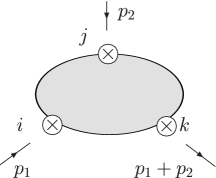
Figure 1: Momentum configuration for the Green functions $\Pi_{123}^{ijk}$.

We are particularly interested in those Green functions that are order parameters of the spontaneous breaking of chiral symmetry. They do not receive contributions from perturbative QCD at large momentum transfer in the chiral limit. As a consequence, their behaviour at short distances is smoother than expected on purely dimensional grounds.

Chiral Ward identities, discrete and $SU(3)$ symmetries constrain the structure of these Green functions [42]. Their short-distance behaviour can be determined within perturbative QCD in terms of an OPE for different kinematical regimes, namely $\Pi(\lambda p_{1},p_{2})$, $\Pi(p_{1},\lambda p_{2})$, $\Pi(\lambda p_{1},\lambda p_{2})$ and $\Pi(\lambda p_{1},p_{2}-\lambda p_{1})$, for large $\lambda$. We will only consider the leading orders both in $1/\lambda$ and in the perturbative expansion of QCD. Consequently, our results hold up to ${\cal O}(\alpha_{S})$ corrections.

The procedure is then straightforward. We first compute the corresponding three-point Green functions within our approach based on the Lagrangian ${\cal L}_{\infty}$. For the different kinematical regimes specified above, we then match the results with those of the OPE. In this way we obtain information on the couplings of the Lagrangian and therefore on the LECs $C_{i}$. The specific details of the matching have to be worked out in each case [16, 17, 18, 20, 21].

5 Resonance exchange for $\mathbf{\langle VAP\rangle}$ and $\mathbf{\langle SPP\rangle}$ correlators

In this section we reanalyse the three-point functions $\langle VAP\rangle$ and $\langle SPP\rangle$ in the present framework. In previous treatments, the chiral resonance approach was either not used at all [21] or with a selected set of couplings only [20].

A virtue of the resonance Lagrangian framework lies in the fact that chiral symmetry is built in from the start. As a consequence the chiral symmetry relations arising at special kinematical points hold automatically and, moreover, the corresponding high-energy behaviour is also inherited. An example is the relation between the $\langle SPP\rangle$ correlator and the $\langle SS-PP\rangle$ two point function discussed in [21]. In the framework of Ref. [21], the relation between $\langle SPP\rangle$ and $\langle SS-PP\rangle$ leads to independent constraints on the chosen ansatz. Here, not only is the relation automatically satisfied but also the high-energy behaviour is correct once the proper high-energy behaviour of the two-point function has been implemented. The relation between the $\langle VA|\pi\rangle$ matrix element and the two-point function $\langle VV-AA\rangle$ is a similar case [16, 17]. This should also be of great advantage for the study of four- and higher-point functions. For this reason the relations in Eqs. (4.1) and (4.1) will be used throughout the present section.

The role of the terms that have been removed by use of field redefinitions is less clear a priori. However, in the examples considered below we demonstrate explicitly that the omission of these terms can be justified by the asymptotic constraints.

5.1 $\langle VAP\rangle$ Green function

Chiral Ward identities, $SU(3)_{V}$, parity and time reversal [16, 17] provide the general expression for the $\langle VAP\rangle$ Green function :

$$(\Pi_{V\!AP})_{\mu\nu}^{ijk}(p,q) = (-2)f^{ijk}\,\Bigg{\{}\,\langle{\overline{\psi}}\psi\rangle_{0}\left[\frac{(p+2q)_{\mu}q_{\nu}}{q^{2}(p+q)^{2}}-\frac{g_{\mu\nu}}{(p+q)^{2}}\right]$$ (5.1)

$$+\,P_{\mu\nu}(p,q)\,{\cal F}(p^{2},q^{2},(p+q)^{2})\,+\,Q_{\mu\nu}(p,q)\,{\cal G}(p^{2},q^{2},(p+q)^{2})\Bigg{\}}\,,$$

where the transverse tensors $P_{\mu\nu}$ and $Q_{\mu\nu}$ are defined by :

$$P_{\mu\nu}(p,q) = q_{\mu}p_{\nu}-(p\cdot q)g_{\mu\nu}\,,$$

$$Q_{\mu\nu}(p,q) = p^{2}q_{\mu}q_{\nu}+q^{2}p_{\mu}p_{\nu}-(p\cdot q)p_{\mu}q_{\nu}-p^{2}q^{2}g_{\mu\nu}\,.$$ (5.2)

The $\langle VAP\rangle$ correlator was studied in Ref. [20] in a resonance Lagrangian framework. In this context the functions $\cal F$ and $\cal G$ were found to be of the general structure

$${\cal F}(p^{2},q^{2},(p+q)^{2}) =\frac{\left\langle\overline{\psi}\psi\right\rangle_{0}}{(p^{2}-M_{V}^{2})(q^{2}-M_{A}^{2})}\,\left[a_{0}\,+\frac{b_{1}\,+\,b_{2}\,p^{2}+\,b_{3}\,q^{2}}{(p+q)^{2}}+\frac{c_{1}\,+\,c_{2}\,p^{2}\,+\,c_{3}\,q^{2}}{(p+q)^{2}-M_{P}^{2}}\right]\,,$$

$${\cal G}((p^{2},q^{2},(p+q)^{2})) =\frac{\left\langle\overline{\psi}\psi\right\rangle_{0}}{(p^{2}-M_{V}^{2})q^{2}}\,\left[\frac{d_{1}\,+\,d_{2}\,q^{2}}{(p+q)^{2}\,(q^{2}-M_{A}^{2})}\,+\,\frac{f}{(p+q)^{2}-M_{P}^{2}}\right]\,.$$ (5.3)

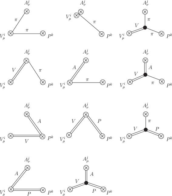
Figure 2: Feynman diagrams contributing to $\Pi_{VAP}$ in the minimal resonance Lagrangian. $\pi$ stands for a Goldstone boson, $V$, $A$ and $P$ denote vector, axial-vector and pseudoscalar resonances, respectively.

The comparison with the present resonance Lagrangian in its minimal form according to subsection 2.3 shows that the analysis of Ref. [20] included all relevant terms with the exception of the three-resonance coupling $\lambda^{VAP}$. In Fig. 2 we show the Feynman diagrams derived from the resonance Lagrangian of Sec. 2 in its minimal form. Since we are also using the same notation for the couplings in the resonance Lagrangian, the results for the coefficients $a_{0},\ldots,f$ may simply be taken over from Ref. [20] except in the case of $c_{1}$ which receives an additional contribution proportional to $\lambda^{VAP}$,

$$c_{1} =-c_{2}M_{V}^{2}-c_{3}M_{A}^{2}\,+\,8\,\lambda^{VAP}\,{F_{V}F_{A}d_{m}}/{F^{2}}\;.$$ (5.4)

The various short-distance conditions discussed in Ref. [20] impose constraints on all but precisely this coefficient,

$$2a_{0}=-b_{2}=2c_{2}=2c_{3}=f=-1\;,\quad b_{3}=d_{2}=0\;,\quad b_{1}=M_{A}^{2}-M_{V}^{2}\;,\quad d_{1}=2M_{A}^{2}~{},$$ (5.5)

implying that the conclusions of Ref. [20] remain unaffected. The predictions for the chiral LECs may be expressed in terms of the coefficients $a_{0},\ldots,f$. Therefore they coincide with the ones of Ref. [20], with the exception of the coupling constant $C_{82}$ that receives a contribution from $\lambda^{VAP}$:

$$C_{82}=-\frac{F^{2}(5M_{V}^{2}+4M_{A}^{2})}{32M_{V}^{4}M_{A}^{2}}-\frac{F^{2}}{32M_{A}^{2}M_{P}^{2}}-\frac{F_{V}F_{A}d_{m}}{2M_{V}^{2}M_{A}^{2}M_{P}^{2}}\,\lambda^{VAP}\;.$$ (5.6)

The predictions for this and the other LECs are of course contained in Table LABEL:tab:RESCi of the present work. Taking into account the restrictions on the resonance couplings imposed by Eq. (5.5), we find, as in Ref. [20]:

$$\sqrt{2}\lambda_{0}=-4\lambda_{1}^{VA}-\lambda_{2}^{VA}-\frac{\lambda_{4}^{VA}}{2}-\lambda_{5}^{VA} =\frac{1}{2\sqrt{2}}(\lambda^{\prime}+\lambda^{\prime\prime})\;,$$ (5.7)

$$\sqrt{2}\lambda^{\prime}=\lambda_{2}^{VA}-\lambda_{3}^{VA}+\frac{\lambda_{4}^{VA}}{2}+\lambda_{5}^{VA} =\frac{M_{A}}{2M_{V}}\;,$$

$$\sqrt{2}\lambda^{\prime\prime}=\lambda_{2}^{VA}-\frac{\lambda_{4}^{VA}}{2}-\lambda_{5}^{VA} =\frac{M_{A}^{2}-2M_{V}^{2}}{2M_{V}M_{A}}\;,$$

$$\lambda_{1}^{PV}=-4\lambda_{2}^{PV}=-\frac{F\sqrt{M_{A}^{2}-M_{V}^{2}}}{4\sqrt{2}d_{m}M_{A}}\;,\quad\lambda_{1}^{PA} =\frac{F\sqrt{M_{A}^{2}-M_{V}^{2}}}{16\sqrt{2}d_{m}M_{V}}\;,$$

where the relations in Eq. (4.1) have been used. Inserting these relations in Table LABEL:tab:RESCi one recovers the predictions for the coupling constants $C_{78}$, $C_{87}$, $C_{88}$, $C_{89}$ and $C_{90}$ in Ref. [20].

One may ask the question what would have become of these results if instead one had performed the calculation with the full resonance Lagrangian before the field redefinitions. We have in fact performed this calculation and the answer to the question is simple: the above result for the $\langle VAP\rangle$ correlator remains valid also in this case. The reason is that the potential additional contributions also lead to conflicts with the OPE and are thus required to vanish.

5.2 $\langle SPP\rangle$ Green function

In Ref. [21] the $\langle SPP\rangle$ Green function was analysed with a general meromorphic ansatz to comply with the large-$N_{C}$ limit of QCD. From $SU(3)_{V}$ and C invariance, the $\langle SPP\rangle$ Green function is given in terms of a single scalar function:

$$\Pi_{SPP}^{ijk}(p,q)\,=\,d^{ijk}\,\Pi_{SPP}\left(p^{2},q^{2},(p+q)^{2}\right)\;.$$ (5.8)

Bose symmetry implies that the function is symmetric in its second and third arguments. According to the results of Ref. [21] it is of the form

$$\Pi_{SPP}(s,t,u)=8B^{3}F^{2}M_{S}^{2}M_{P}^{4}\frac{1+P_{1}+P_{2}+P_{3}+P_{4}}{[M_{S}^{2}-s][-t][-u][M_{P}^{2}-t][M_{P}^{2}-u]}\;,$$ (5.9)

where the $P_{n}$ are polynomials of degree $n$ in the variables $s$, $t$ and $u$

$$P_{1} =c_{010}(t+u)\;,$$ (5.10)

$$P_{2} =c_{011}tu\;,$$

$$P_{3} =[c_{111}s+c_{021}(t+u)]tu\;,$$

$$P_{4} =[c_{211}(s^{2}-(t-u)^{2})+c_{121}(s(t+u)-(t-u)^{2})]tu\;.$$

As discussed in Ref. [21], the restrictions on the form of the polynomials arise from the requirements that the asymptotic behaviour of the function $\Pi_{SPP}$ in the various limits be no worse than what follows from the OPE and that the scalar and pseudoscalar (transition) form factors with at least one pion vanish asymptotically.

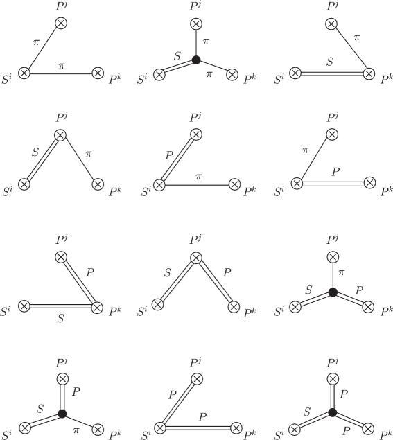
Figure 3: Feynman diagrams contributing to $\Pi_{SPP}$ in the minimal resonance Lagrangian. $\pi$ stands for a Goldstone boson, $S$ and $P$ denote scalar and pseudoscalar resonances, respectively.

The computation within the chiral resonance framework in its minimal version according to subsection 2.3 is straightforward. The relevant diagrams are given in Fig. 3 and they yield the result

$$\Pi_{SPP}(p_{1}^{2},p_{2}^{2},q^{2}) = -\,64\,B^{3}\,\Bigg{\{}\,\frac{-F^{2}}{8\,q^{2}\,p_{2}^{2}}+\frac{c_{m}^{2}}{p_{1}^{2}-M_{S}^{2}}\left(\frac{1}{q^{2}}+\frac{1}{p_{2}^{2}}\right)$$ (5.11)

$$-\,d_{m}^{2}\left(\frac{1}{q^{2}\left(p_{2}^{2}-M_{P}^{2}\right)}+\frac{1}{p_{2}^{2}\left(q^{2}-M_{P}^{2}\right)}\right)-\frac{c_{m}\,c_{d}\,q\cdot p_{2}}{q^{2}p_{2}^{2}\left(p_{1}^{2}-M_{S}^{2}\right)}$$

$$+\frac{2\,c_{m}\,d_{m}\,\lambda^{SP}_{1}}{p_{1}^{2}-M_{S}^{2}}\left(-\frac{q\cdot p_{1}}{q^{2}\left(p_{2}^{2}-M_{P}^{2}\right)}+\frac{p_{1}\cdot p_{2}}{p_{2}^{2}\left(q^{2}-M_{P}^{2}\right)}\right)$$

$$+\frac{4c_{m}\,d_{m}\,\lambda^{SP}_{2}}{p_{1}^{2}-M_{S}^{2}}\left(\frac{1}{q^{2}-M_{P}^{2}}+\frac{1}{p_{2}^{2}-M_{P}^{2}}\right)$$

$$+\frac{4\,d_{m}^{2}\,\lambda^{PP}_{3}}{\left(q^{2}-M_{P}^{2}\right)\left(p_{2}^{2}-M_{P}^{2}\right)}-\frac{4\,c_{m}\,d_{m}^{2}\,\lambda^{SPP}}{\left(p_{1}^{2}-M_{S}^{2}\right)\left(q^{2}-M_{P}^{2}\right)\left(p_{2}^{2}-M_{P}^{2}\right)}\Bigg{\}}\,.$$

In addition to the couplings from the Lagrangian ${\cal L}_{(2)}^{R}$ in Eq. (2.2), $\Pi_{SPP}$ is found to depend on the resonance couplings $\lambda_{i}^{SP}~{}(i=1,2)$, $\lambda_{3}^{PP}$ and $\lambda^{SPP}$. Inspection reveals that this result is of the desired form, up to a contribution $\propto(\lambda^{SP}_{1}+d_{m}/c_{m})(s(t+u)-t^{2}-u^{2})$ to $P_{2}$ that is in conflict with demanding that the scalar form factor involving a Goldstone boson and a pseudoscalar resonance fades away at high momenta. The conflict is resolved by the condition

$$\lambda_{1}^{SP}=-\displaystyle\frac{d_{m}}{c_{m}}~{}.$$ (5.12)

Inserting this relation in Table LABEL:tab:RESCi along with the relations in Eq. (4.1) one recovers the predictions for $C_{12}$, $C_{34}$ and $C_{38}$ from Ref. [21].

In the resonance Lagrangian approach a new feature arises. The OPE expansion for the $\langle SPP\rangle$ function demands that its leading term behaves as $\Pi_{SPP}(\lambda^{2}s,\lambda^{2}t,\lambda^{2}u)\sim{\cal O}(1/\lambda^{2})$, while one can see that our result of Eq. (5.11) is of ${\cal O}(1/\lambda^{4})$. This should come as no surprise since the terms with the potential to generate ${\cal O}(1/\lambda^{2})$ contributions to the $\langle SPP\rangle$ Green function ($\lambda^{S}_{8,14}$ and $\lambda^{P}_{6,10}$) have been discarded when constructing the minimal resonance Lagrangian. It turns out, however, that the attempt to generate $c_{211},c_{121}\neq 0$ by retaining those terms is bound to fail because the restrictions imposed by Eq. (5.10) require $\lambda^{S}_{8}=\lambda^{S}_{14}=\lambda^{P}_{6}=\lambda^{P}_{10}=0$ nonetheless. (Note that there arise contributions proportional to $\lambda^{S}_{8}(t^{3}+u^{3})$ and $\lambda^{P}_{6}s^{2}(t+u)$ in $P_{3}$.)

It is relevant to notice that, as already commented in Ref. [21], the procedure we are devising does not apply to all Green functions with the same settings. Contrary to the $\langle VAP\rangle$ case, higher-order corrections furnish the Wilson coefficients of the $\langle SPP\rangle$ function with anomalous dimensions and therefore the matching in the $N_{C}\rightarrow\infty$ limit that we intend to enforce (with a finite number of meson states in the spectrum) is not fully feasible in the $\langle SPP\rangle$ case. Thus we take the softer approach of demanding that asymptotically our Green functions behave no worse than given by the OPE expansion at leading order, as implemented in Ref. [21].

6 Conclusions

The LECs of $\chi$PT encode the dynamical information on the massive hadronic states of QCD, which are not present explicitly in the effective Goldstone Lagrangian. The most important contributions to the LECs are expected to originate from the low-lying mesonic resonances because contributions from heavier hadrons are suppressed by inverse powers of their masses.

In the large-$N_{C}$ limit of QCD, the correlators of colour-singlet quark-antiquark currents are given by tree-level exchanges of infinite towers of narrow mesons. Crossing and unitarity imply that these sums correspond to the lowest-order approximation of some effective mesonic Lagrangian. The construction of this general Lagrangian, with an infinite number of hadronic states, is beyond our present abilities. However, truncating the hadronic spectrum to the lowest-lying multiplets with $J^{PC}=1^{--},1^{++},0^{-+}$ and $0^{++}$, one obtains a very good approximation at low energies. The couplings of this resonance Lagrangian should be determined by imposing that the corresponding Green functions reproduce the asymptotic behaviour of QCD_∞. Integrating out all massive fields at the level of the generating functional, one obtains the low-energy effective Lagrangian of the Goldstone modes. Therefore, from the resonance chiral Lagrangian one can determine the LECs of $\chi$PT as functions of resonance parameters.

In this paper we have constructed the most general $SU(3)_{L}\times SU(3)_{R}$ invariant Lagrangian, containing Goldstone bosons and the lowest-lying $J^{PC}=1^{--},1^{++},0^{-+}$ and $0^{++}$ multiplets, that contributes to ${\cal L}_{6}^{\rm\chi PT}$ after integrating out the resonance fields. Since any resonance exchange involves a suppression factor $1/M_{R}^{2}$ from the resonance propagator, we only need to consider terms involving one, two or three resonance fields, coupled to chiral monomials of ${\cal O}(p^{4})$, ${\cal O}(p^{2})$ and ${\cal O}(p^{0})$, respectively. This can also be seen by expanding the classical equations of motion of the resonance fields in inverse powers of the heavy masses, which shows that for $p^{2}\ll M_{R}^{2}$ the resonance fields scale as $R\sim{\cal O}(p^{2}/M_{R}^{2})$.

The number of possible chiral structures is rather large. Using partial integration, the lowest-order equations of motion and algebraic identities to eliminate linearly dependent terms, we have identified a basis of 70 monomials in ${\cal L}^{R}_{(4)}$, 38 in ${\cal L}^{RR}_{(2)}$ and 7 in ${\cal L}^{RRR}_{(0)}$. This basis is, however, highly redundant for the purpose of determining the LECs of ${\cal O}(p^{6})$ because only certain combinations of the resonance couplings occur in the LECs. This can be understood through appropriate redefinitions of the resonance fields that leave the generating functional invariant. We have found a large number of linear field redefinitions of the type (2.20), allowing us to eliminate 47 terms of the resonance Lagrangian ${\cal L}^{R}_{(4)}$ by transforming them into structures of higher chiral order that do not contribute to ${\cal L}_{6}^{\rm\chi PT}$. We have chosen to eliminate preferentially terms with $\chi$’s, while keeping those with many derivatives. Higher-derivative structures generate a worse short-distance behaviour and, therefore, will be most easily eliminated through high-energy QCD constraints. In fact, six surviving operators can be discarded because they induce an unacceptable high-energy behaviour of two-point functions. In addition, there are two constants in ${\cal L}^{R}_{(4)}$ that only lead to contributions subleading in $1/N_{C}$. We have finally kept a total of 15 terms in ${\cal L}^{R}_{(4)}$: four vector, three axial-vector, five scalar and three pseudoscalar operators.

Once the relevant resonance Lagrangian has been determined, we have performed the functional integration of the resonance fields and obtained their contribution to the LECs of ${\cal O}(p^{6})$. The results, given in App. D, still show the presence of redundant terms; many resonance couplings appear only in definite combinations. Again, this can be understood through additional non-linear field redefinitions of the type (2.24), which could be used to eliminate all seven trilinear couplings and six bilinear operators. One further bilinear coupling can be dismissed on the basis of large $N_{C}$. Altogether, 46 independent combinations of resonance couplings appear in the LECs of ${\cal O}(p^{6})$.

We have adopted the usual chiral formulation of spin-1 fields in terms of antisymmetric tensors. For completeness, we have added possible contributions to ${\cal L}_{6}^{\rm\chi PT}$ from odd-parity vector and axial-vector terms, with ${\cal O}(p^{3})$ chiral monomials in the Proca field formulation. This introduces three additional couplings, not present in the antisymmetric formalism at this order in the momentum expansion. The equivalence of different formalisms for vector fields, once short-distance constraints are taken into account, was demonstrated at ${\cal O}(p^{4})$ in Ref. [11]. One of the three Proca-type couplings contributing at ${\cal O}(p^{6})$ is already known to be nonvanishing [32]. In the antisymmetric tensor formulation, corresponding local terms of ${\cal O}(p^{6})$ would have to be added to the chiral resonance Lagrangian. For the other two couplings, a short-distance analysis remains to be done.

The large-$N_{C}$ counting is more transparent in the $U(3)_{L}\times U(3)_{R}$ effective theory, where multiple-trace terms are suppressed by corresponding powers of $1/N_{C}$. However, one needs then to consider the special role of the $U(1)_{A}$ anomaly, which is a very important physical effect not present at leading order in $1/N_{C}$. This can be incorporated through a more involved counting in powers of $p^{2}\sim m_{q}\sim 1/N_{C}$. Integrating out the singlet Goldstone field, one recovers the more standard $SU(3)_{L}\times SU(3)_{R}$ chiral framework. This procedure is sketched in App. A, hereby elucidating the role of the multiple-trace terms encountered in our resonance Lagrangian. A more systematic analysis of the $\eta^{\prime}$ contributions to the ${\cal O}(p^{6})$ LECs will be given in [25].

The complete list of resonance contributions to the chiral couplings of ${\cal O}(p^{6})$ constitutes our main result. It shows which LECs are not sensitive at all to resonance exchange and, therefore, may be expected to be negligible. Moreover, there are interesting relations among different couplings, which can be useful for phenomenological applications, e.g., $C_{20}=-3C_{21}=C_{32}=C_{35}/6=C_{94}/8$ or $C_{24}=6C_{28}=3C_{30}$, etc. In a few cases, e.g., $C_{1}+4C_{3}$, $3C_{1}-4C_{4}$, $C_{12}$, $C_{1}/12-C_{28}+r_{S}C_{32}$, $C_{38}$, $C_{87}$, $C_{88}-C_{90}$, $C_{91}$, $C_{93}$, etc., the ${\cal O}(p^{6})$ LECs only depend on resonance couplings already present at ${\cal O}(p^{4})$.

Our program towards a systematic analysis of resonance contributions still involves a missing step: the determination of the resonance couplings through appropriate short-distance QCD constraints. These couplings could be fixed by enforcing a systematic matching procedure between the Green functions of QCD_∞ and their corresponding correlators in the effective low-energy theory. The matching cannot be exact, i.e. it is not possible to perform it for all possible Green functions, because that would require to introduce an infinite number of hadronic states. Nevertheless, it is certainly possible to accomplish a matching good enough to correctly describe a wide set of interesting physical observables. We have shown two known examples, the $\langle VAP\rangle$ and $\langle SPP\rangle$ three-point functions, which provide very useful constraints on some low-energy couplings. A thorough study of other three-point correlators is under way.

Appendix A Multiple-trace terms and $\eta^{\prime}$ exchange

The form of the EOM (2.14) implies that the number of traces is not conserved over the course of constructing the effective Lagrangian. In principle, this could be circumvented at the cost of ignoring the EOM and writing the Lagrangian in terms of $\nabla_{\mu}u^{\mu}$. More fundamentally, this circumstance reflects the fact that the counting of traces in the effective theory is in general not in direct correspondence with the order in $1/N_{C}$ of a term .

This discrepancy is generated by the occurrence of an intermediate singlet pseudoscalar (the $\eta^{\prime}$) which in the present context is treated as massive, as is reflected by the Goldstone manifold being $SU(3)$. To arrive at a classification of contributions with respect to their order in $1/N_{C}$ one should instead start from a Lagrangian which involves the singlet field as an explicit degree of freedom. In this case the leading-order Lagrangian reads [43]

$$\tilde{{\cal L}}=\frac{{F}_{0}^{2}}{4}\langle\tilde{u}_{\mu}\tilde{u}^{\mu}+\tilde{\chi}_{+}\rangle+\frac{{F}_{0}^{2}}{3}M_{0}^{2}\ln^{2}(\det\tilde{u}),$$ (A.1)

where the tildes refer to building blocks made of an effective field $\tilde{u}(x)\in U(3)$. The additional degree of freedom, $\ln(\det\tilde{u})$, comes with a nonzero chiral limit mass $M_{0}$ that prevents it from causing a ‘$U(1)$ problem’ [44]. It is well known, however, that this mass vanishes in the large-$N_{C}$ limit, $M_{0}^{2}={\cal O}(1/N_{C})$. The structure of the above effective Lagrangian implies a balance between the scales set by the momenta, quark masses and $1/N_{C}$ ,

$$p^{2}\sim m_{q}\sim M_{0}^{2}\,.$$ (A.2)

The validity of the theory relies on the assumption that all of these scales are small in comparison to the intrinsic scale of QCD. While that is a nontrivial assumption, the benefit lies in the fact that the large-$N_{C}$ counting rules are now ‘canonical’: terms with single traces are of order $N_{C}$ while additional traces reduce the order in $1/N_{C}$ by unity. Factors of $\ln(\det\tilde{u})$ also lead to a suppression in $1/N_{C}$, which can be understood in a framework where singlet external fields are present [30, 31, 45].

Contact with the standard effective theory is established when treating the mass $M_{0}^{2}$ as large in comparison to the octet meson masses and momenta squared, such that by the EOM

$$\tilde{u}=u\{1+\frac{1}{12M_{0}^{2}}\langle\chi_{-}\rangle+{\cal O}(p^{4})\},$$ (A.3)

with $\det u=1$. Proceeding in this manner, one recovers the well-known $\eta^{\prime}$ contribution to the coupling constant $L_{7}$ [3],

$$L_{7}^{(\eta^{\prime})}=-\frac{F_{0}^{2}}{48M_{0}^{2}}\,.$$ (A.4)

As emphasized in Refs. [3, 23], some care is needed in performing the large-$N_{C}$ limit for $L_{7}$, that is still an open question. We refer to Refs. [24, 25] for detailed expositions in which sense $L_{7}$ can be counted as ${\cal O}(N_{C}^{2})$ even though it is the coefficient of the double-trace term $\langle\chi_{-}\rangle^{2}$. On the other hand, contributions to $L_{1}-\frac{1}{2}L_{2}$, $L_{4}$ and $L_{6}$ do not occur. These LECs are therefore booked as ${\cal O}(1)$ at large-$N_{C}$, in accordance with the double-trace structure of the corresponding monomials in the chiral $SU(3)$ Lagrangian of ${\cal O}(p^{4})$ [3].

Similarly, one also has the possibility to set up a resonance Lagrangian in the framework where the singlet field is explicitly present [31]. Apart from additional terms that involve factors of $\ln(\det\tilde{u})$ one has terms of the same form as those in Eq. (2.2). Proceeding as above one generates the following multiple-trace terms,

$$c_{m}\langle S\tilde{\chi}_{+}\rangle \rightarrow c_{m}\langle S{\chi}_{+}\rangle-\frac{c_{m}}{6M_{0}^{2}}\langle S{\chi}_{-}\rangle\langle\chi_{-}\rangle+\ldots$$ (A.5)

$$c_{d}\langle S\tilde{u}_{\mu}\tilde{u}^{\mu}\rangle \rightarrow c_{d}\langle S{u}_{\mu}{u}^{\mu}\rangle+\frac{c_{d}}{3M_{0}^{2}}i\langle Su_{\mu}\rangle\partial^{\mu}\langle\chi_{-}\rangle+\ldots$$

$$i\,d_{m}\langle P\tilde{\chi}_{-}\rangle \rightarrow i\,d_{m}\langle P{\chi}_{-}\rangle-\frac{d_{m}}{6M_{0}^{2}}i\langle P{\chi}_{+}\rangle\langle\chi_{-}\rangle+\ldots~{},$$

which are obviously in direct correspondence to those generated by the application of the EOM in Eq. (2.14). Again the occurrence of the factor $M_{0}^{-2}={\cal O}(N_{c})$ leads to an enhancement in $1/N_{C}$, which is why we do not dispose of those terms. In an accompanying paper [25], the $\eta^{\prime}$ contributions to the LECs of ${\cal O}(p^{4})$ [3] and ${\cal O}(p^{6})$ are studied in a more systematic manner.

In the following we discuss in more detail how one arrives at our effective Lagrangian if one starts from a resonance Lagrangian including the $\eta^{\prime}$. In the diagram below, this Lagrangian sits in the upper left corner ($\tilde{\cal L}_{{\rm eff}}^{\cal R}$):

$$\tilde{\cal L}_{{\rm eff}}^{\cal R}\quad\overset{\eta^{\prime}/}{\longrightarrow}\quad{\cal L}_{{\rm eff}}^{\cal R(\eta^{\prime})}$$

$$\downarrow{\cal R/}\hskip 50.00008pt\downarrow{\cal R/}$$ (A.6)

$$\tilde{\cal L}_{{\rm eff}}^{(\cal R)}\quad\overset{\eta^{\prime}/}{\longrightarrow}\quad{\cal L}_{{\rm eff}}^{\cal(\eta^{\prime},R)}$$

The notation is the following: a superscript ${\cal R}$ denotes a Lagrangian with explicit resonance fields, whereas superscripts in brackets denote contributions from the resonances and/or $\eta^{\prime}$ in the coupling constants. The presence of the $\eta^{\prime}$ (the chiral group being $U(3)$) is indicated by a tilde ($\tilde{\quad}$). A slash (/) symbolizes the process of integrating out a field. The final effective Lagrangian of this work is ${\cal L}_{{\rm eff}}^{\cal(\eta^{\prime},R)}$ in the lower right corner. Here, we want to analyse the transition from the upper left to the upper right.

Let us start with the low-energy expansion of $\tilde{\cal L}_{{\rm eff}}^{\cal R}$. As indicated above, the relevant expansion is the one where powers of momenta, quark masses and $1/N_{C}$ are treated as small, according to

$$p^{2}\sim m_{q}\sim 1/N_{C}={\cal O}(\delta),$$ (A.7)

where a counting parameter $\delta$ has been introduced [30]. The expansion for our Lagrangian thus takes the form

$$\tilde{\cal L}_{{\rm eff}}^{\cal R}=\tilde{\cal L}_{0}^{\cal R}+\tilde{\cal L}_{1}^{\cal R}+\tilde{\cal L}_{2}^{\cal R}+O(\delta^{3}).$$ (A.8)

The leading-order term $\tilde{\cal L}_{0}^{\cal R}$ is of course nothing but the Lagrangian $\tilde{\cal L}$ in (A.1) and it is in fact independent of the resonance fields ${\cal R}$. The term $\tilde{\cal L}_{1}^{\cal R}$ has been given in Ref. [31] and involves several terms of order $N_{C}p^{4}$ as well as one contribution (in $\tilde{\cal L}_{1}^{P}$) of order $N_{C}^{0}p^{2}$ proportional to $\ln(\det\tilde{u})\,\langle P\rangle$, viz.

$$\tilde{\cal L}_{1}^{P}=\ldots-2id_{0}\ln(\det\tilde{u})\,\langle P\rangle.$$ (A.9)

Here, the resonance fields have implicitly been counted as order $\sqrt{N_{C}}p^{2}$. The factor of $\sqrt{N_{C}}$ arises simply because of the normalization of the resonance fields, whereas the power of $p^{2}$ can be understood when treating the resonance masses as large (i.e. of order $1$) and solving the EOM. In simplifying the expression for the Lagrangian $\tilde{\cal L}_{1}^{\cal R}$, the EOM for the Goldstone fields has been used to eliminate terms involving $\nabla_{\mu}\tilde{u}^{\mu}$. In the present case it takes the form

$$2\nabla_{\mu}\tilde{u}^{\mu}=i\tilde{\chi}_{-}-\frac{4i}{3}M_{0}^{2}\ln\det\tilde{u}$$ (A.10)

as one derives from the Lagrangian (A.1).

We now consider the terms of ${\cal O}(\delta^{2})$. The Lagrangian $\tilde{\cal L}_{2}^{\cal R}$ collects the contributions of order $N_{C}p^{6}$, $N_{C}^{0}p^{4}$ and $N_{C}^{-1}p^{2}$,

$$\tilde{\cal L}_{2}^{\cal R}=\tilde{\cal L}_{2}^{\cal R}|_{N_{C}p^{6}}+\tilde{\cal L}_{2}^{\cal R}|_{N_{C}^{0}p^{4}}+\tilde{\cal L}_{2}^{\cal R}|_{N_{C}^{-1}p^{2}}.$$ (A.11)

The recipe to determine the first of these terms is to consult the tables of the present paper and identify all the terms that only involve a single trace; in those replace the effective field $u$ by $\tilde{u}$ and, finally, equip the associated coupling constants with tildes, i.e.

$$\tilde{\cal L}_{2}^{\cal R}|_{N_{C}p^{6}}=\tilde{\lambda}^{V}_{1}i\langle V_{\mu\nu}\tilde{u}^{\mu}\tilde{u}_{\alpha}\tilde{u}^{\alpha}\tilde{u}^{\nu}\rangle+\ldots$$ (A.12)

with all the above $\tilde{\lambda}^{R}_{i}={\cal O}(\sqrt{N_{C}})$. We will not attempt to give the next term explicitly, but simply indicate exemplary contributions:

$$\tilde{\cal L}_{2}^{\cal R}|_{N_{C}^{0}p^{4}} =\tilde{\lambda}^{S}_{n}\langle{S}\rangle\langle\tilde{\chi}_{+}\rangle+\ldots+\tilde{\lambda}^{S}_{n^{\prime}}\langle{S}\rangle^{2}+\ldots+\tilde{\lambda}^{S}_{n^{\prime\prime}}\ln\det\tilde{u}\langle{S}\tilde{\chi}_{-}\rangle+\ldots,$$

$$\tilde{\lambda}^{S}_{n(^{\prime}(^{\prime}))} ={\cal O}(N_{C}^{-\frac{1}{2}}).$$ (A.13)

Finally, the last piece of the ${\cal O}(\delta^{2})$ Lagrangian consists of a single term

$$\tilde{\cal L}_{2}^{\cal R}|_{N_{C}^{-1}p^{2}} =\tilde{\lambda}^{S}_{m}\ln^{2}(\det\tilde{u})\langle S\rangle,$$ (A.14)

with $\tilde{\lambda}^{S}_{m}={\cal O}(N_{C}^{-\frac{3}{2}})$. Again, the EOM has been used to eliminate $\nabla_{\mu}\tilde{u}^{\mu}$ terms. The difference to the standard framework lies in the fact that the application of the EOM does not generate factors of $\langle\chi_{-}\rangle$ but instead factors of $\ln\det\tilde{u}$ and thereby intertwines the three types of contributions to $\tilde{\cal L}_{2}^{\cal R}$.

Let us now turn to the transition from the upper left to the upper right of our diagram. There are several contributions to be considered:

1. When integrating out the $\eta^{\prime}$ the term $\tilde{\cal L}_{0}^{\cal R}=\tilde{\cal L}$ generates several purely $\eta^{\prime}$ contributions to low-energy constants, $L_{7}^{(\eta^{\prime})}$ is an example. For these we refer to Ref. [25].

2. In the Lagrangian $\tilde{\cal L}_{1}^{\cal R}$ the first class of contributions is generated by replacing the field $\tilde{u}$ by $u$ which produces the Lagrangian (2.2). Note that the difference of $\tilde{u}$ and $u$ is of order $p^{2}$ when the $\eta^{\prime}$ mass $M_{0}$ is treated as large.

3. Retaining terms up to ${\cal O}(p^{6})$ only, the three terms generated by that difference are those given in Eq. (A.5).

4. These would have been all contributions from $\tilde{\cal L}_{1}^{\cal R}$ would it not be for the term $\propto d_{0}$ in Eq. (A.9). Closer inspection reveals, however, that contributions of this term can be neglected without significant loss of information because it exclusively leads to nonleading contributions in $1/N_{C}$. This can be seen from the solution of the singlet field’s EOM,

   $$\ln\det\tilde{u}=\frac{1}{4M_{0}^{2}}\{\langle\chi_{-}\rangle+\frac{12id_{0}}{F_{0}^{2}}\langle{P}\rangle\}+{\cal O}(p^{4}).$$ (A.15)

   Upon integrating out the pseudoscalar resonance $P$, $d_{0}$ generates a contribution $\propto\langle\chi_{-}\rangle$, relatively suppressed by $d_{0}d_{m}/F_{0}^{2}={\cal O}(1/N_{C})$.

5. It remains to work out the contributions from $\tilde{\cal L}_{2}^{\cal R}$. Again, the singly traced ${\cal O}(N_{C}p^{6})$ terms are in direct correspondence with the single-trace terms in the tables of the present work. For these one finds the trivial matching relations

   $$\lambda^{R}_{i} =\tilde{\lambda}^{R}_{i}.$$ (A.16)

   As far as the remaining terms are concerned they either lead to genuinely suppressed contributions ($\tilde{\lambda}^{S}_{n},\tilde{\lambda}^{S}_{n^{\prime}}$, etc.) or to contributions that are suppressed relatively to the leading $\eta^{\prime}$ exchange contributions. For instance, the contribution of $\tilde{\lambda}^{S}_{m}\ln^{2}(\det\tilde{u})\langle{S}\rangle$ to the term $\langle\chi_{-}\rangle^{2}\langle\chi_{+}\rangle$ is of ${\cal O}(N_{C})$, whereas the leading-order contributions to this term are of ${\cal O}(N_{C}^{3})$ [25]. For this reason we will simply neglect these terms altogether.

To summarize, the transition from the upper left to the upper right of our diagram has lead to a resonance Lagrangian that consists of single-trace terms only, up to three double-trace terms ${\cal O}^{S}_{4}$, ${\cal O}^{S}_{5}$ and ${\cal O}^{P}_{3}$ as given explicitly in Eq. (A.5).

Appendix B Field redefinitions

In this appendix we report some details of our analysis of linear field redefinitions. Let us start by listing the allowed redefinitions for resonance fields.

Redefinitions for vector meson fields

$$1)\qquad V_{\mu\nu} \longrightarrow V_{\mu\nu}\,+\,g\,\left[\,A_{\mu\nu}\,,\,\chi_{-}\,\right]\;,$$

$$2)\qquad V_{\mu\nu} \longrightarrow V_{\mu\nu}\,+\,i\,g\,\left(\,\left[\,A_{\mu\alpha}\,,\,f_{-\beta\nu}\,\right]\,-\,\left[\,A_{\nu\alpha}\,,\,f_{-\beta\mu}\,\right]\,\right)\,g^{\alpha\beta}\;,$$

$$3)\qquad V_{\mu\nu} \longrightarrow V_{\mu\nu}\,+\,i\,g\,\left(\,\left[\,A_{\nu\alpha}\,,h_{\mu}^{\alpha}\,\right]\,-\,\left[\,A_{\mu\alpha}\,,\,h_{\nu}^{\alpha}\,\right]\,\right)\,\;,$$

$$4)\qquad V_{\mu\nu} \longrightarrow V_{\mu\nu}\,+\,i\,g\,\left(\,\left[\,\nabla_{\mu}P\,,\,u_{\nu}\,\right]\,-\,\left[\,\nabla_{\nu}P\,,\,u_{\mu}\,\right]\,\right)\;,$$

$$5)\qquad V_{\mu\nu} \longrightarrow V_{\mu\nu}\,+\,i\,g\,\left[\,P\,,\,f_{-\mu\nu}\,\right]\,,$$

$$6)\qquad V_{\mu\nu} \longrightarrow V_{\mu\nu}\,+\,i\,g\,\left\{\,S\,,\,\left[\,u_{\mu}\,,\,u_{\nu}\,\right]\,\right\}\;,$$

$$7)\qquad V_{\mu\nu} \longrightarrow V_{\mu\nu}\,+\,g\,\left\{\,S\,,\,f_{+\mu\nu}\,\right\}\;,$$

$$8)\qquad V_{\mu\nu} \longrightarrow V_{\mu\nu}\,+\,ig\,\left(u_{\mu}\,S\,u_{\nu}\,-u_{\nu}\,S\,u_{\mu}\right)\;,$$

$$9)\qquad V_{\mu\nu} \longrightarrow V_{\mu\nu}\,+\,g\,\left\{\,V_{\mu\nu}\,,\,u_{\alpha}\,u^{\alpha}\,\right\}\ ,$$ (B.1)

$$10)\qquad V_{\mu\nu} \longrightarrow V_{\mu\nu}\,+\,g\,\left\{\,V_{\mu\nu}\,,\chi_{+}\,\right\}\,\;,$$

$$11)\qquad V_{\mu\nu} \longrightarrow V_{\mu\nu}\,+\,g\ u_{\alpha}\,V_{\mu\nu}\,u^{\alpha}\,\;,$$

$$12)\qquad V_{\mu\nu} \longrightarrow V_{\mu\nu}\,+\,i\,g\,\left(\,\left[f_{+\mu\alpha}\,,\,V_{\beta\nu}\right]\,-\,\left[f_{+\nu\alpha}\,,\,V_{\beta\mu}\right]\,\right)\,g^{\alpha\beta}\,\;,$$

$$13)\qquad V_{\mu\nu} \longrightarrow V_{\mu\nu}\,+\,g\,\left(\,u^{\alpha}\,V_{\mu\alpha}\,u_{\nu}\,+\,u_{\nu}\,V_{\mu\alpha}\,u^{\alpha}\,-\,\,u^{\alpha}\,V_{\nu\alpha}\,u_{\mu}\,-\,u_{\mu}\,V_{\nu\alpha}\,u^{\alpha}\,\right)\,\;,$$

$$14)\qquad V_{\mu\nu} \longrightarrow V_{\mu\nu}\,+\,g\,\left(\,\left[\,\left[u_{\mu},u^{\alpha}\right]\,,\,V_{\nu\alpha}\,\right]\,-\,\left[\,\left[u_{\nu},u^{\alpha}\right]\,,\,V_{\mu\alpha}\,\right]\,\right)\,\;,$$

$$15)\qquad V_{\mu\nu} \longrightarrow V_{\mu\nu}\,+\,g\,\left(\,\{\,\{u_{\mu},u^{\alpha}\}\,,\,V_{\nu\alpha}\,\}\,-\,\{\,\{u_{\nu},u^{\alpha}\}\,,\,V_{\mu\alpha}\,\}\,\right)\,\;,$$

$$16)\qquad V_{\mu\nu} \longrightarrow V_{\mu\nu}\,+\,i\,g\,\left(\,\left[\,\nabla_{\mu}\,A_{\nu\alpha}\,-\,\nabla_{\nu}\,A_{\mu\alpha}\,,\,u^{\alpha}\,\right]\,\right)\,\;,$$

$$17)\qquad V_{\mu\nu} \longrightarrow V_{\mu\nu}\,+\,i\,g\,\left[\,\nabla_{\alpha}\,A_{\mu\nu}\,,\,u^{\alpha}\,\right]\,\;,$$

$$18)\qquad V_{\mu\nu} \longrightarrow V_{\mu\nu}\,+\,i\,g\,\left(\,\left[\,\nabla^{\alpha}\,A_{\alpha\nu}\,,\,u_{\mu}\,\right]\,-\,\left[\,\nabla^{\alpha}\,A_{\alpha\mu}\,,\,u_{\nu}\,\right]\,\right)\,\;.$$

Redefinitions for scalar fields

$$1)\qquad S \longrightarrow S\,+\,g\,\left\{\,\nabla_{\mu}A^{\mu\nu}\,,\,u_{\nu}\,\right\}\,\;,$$

$$2)\qquad S \longrightarrow S\,+\,g\,\left\{\,A^{\mu\nu}\,,\,f_{-\mu\nu}\,\right\}\;,$$

$$3)\qquad S \longrightarrow S\,+\,i\,g\,\left\{\,V^{\mu\nu}\,,\,u_{\mu}\,u_{\nu}\,\right\}\;,$$

$$4)\qquad S \longrightarrow S\,+\,g\,\left\{\,V^{\mu\nu}\,,\,f_{+\mu\nu}\,\right\}\;,$$

$$5)\qquad S \longrightarrow S\,+\,i\,g\,u_{\mu}\,V^{\mu\nu}\,u_{\nu}\;,$$

$$6)\qquad S \longrightarrow S\,+\,g\,\left\{\,\nabla_{\mu}P\,,\,u^{\mu}\,\right\}\;,$$ (B.2)

$$7)\qquad S \longrightarrow S\,+\,i\,g\,\left\{\,P\,,\,\chi_{-}\,\right\}\;,$$

$$8)\qquad S \longrightarrow S\,+\,i\,g\,P\,\left\langle\,\chi_{-}\,\right\rangle\;,$$

$$9)\qquad S \longrightarrow S\,+\,g\,\left\{\,S\,,\,u_{\alpha}\,u^{\alpha}\,\right\}\;,$$

$$10)\qquad S \longrightarrow S\,+\,g\,\left\{\,S\,,\chi_{+}\,\right\}\,\;,$$

$$11)\qquad S \longrightarrow S\,+\,g\ u_{\alpha}\,S\,u^{\alpha}\,\;.$$

Redefinitions for axial-vector fields

$$1)\qquad A_{\mu\nu} \longrightarrow A_{\mu\nu}\,+\,g\,\left[\,V_{\mu\nu}\,,\,\chi_{-}\,\right]\;,$$

$$2)\qquad A_{\mu\nu} \longrightarrow A_{\mu\nu}\,+\,i\,g\,\left(\,\left[\,V_{\mu\alpha}\,,\,f_{-\beta\nu}\,\right]\,-\,\left[\,V_{\nu\alpha}\,,\,f_{-\beta\mu}\,\right]\,\right)\,g^{\alpha\beta}\;,$$

$$3)\qquad A_{\mu\nu} \longrightarrow A_{\mu\nu}\,+\,i\,g\,\left(\,\left[\,V_{\nu\alpha}\,,h_{\mu}^{\alpha}\,\right]\,-\,\left[\,V_{\mu\alpha}\,,\,h_{\nu}^{\alpha}\,\right]\,\right)\,\;,$$

$$4)\qquad A_{\mu\nu} \longrightarrow A_{\mu\nu}\,+\,i\,g\,\left[\,P\,,\,f_{+\mu\nu}\,\right]\;,$$

$$5)\qquad A_{\mu\nu} \longrightarrow A_{\mu\nu}\,+\,g\,\left[\,P\,,\,\left[\,u_{\mu}\,,\,u_{\nu}\,\right]\,\right]\;,$$

$$6)\qquad A_{\mu\nu} \longrightarrow A_{\mu\nu}\,+\,g\,\left(\,\left\{\,\nabla_{\mu}S\,,\,u_{\nu}\,\right\}\,-\,\left\{\,\nabla_{\nu}S\,,\,u_{\mu}\,\right\}\,\right)\;,$$

$$7)\qquad A_{\mu\nu} \longrightarrow A_{\mu\nu}\,+\,g\,\left\{\,S\,,\,f_{-\mu\nu}\,\right\}\;,$$

$$8)\qquad A_{\mu\nu} \longrightarrow A_{\mu\nu}\,+\,g\,\left\{\,A_{\mu\nu}\,,\,u_{\alpha}\,u^{\alpha}\,\right\}\;,$$

$$9)\qquad A_{\mu\nu} \longrightarrow A_{\mu\nu}\,+\,g\,\left\{\,A_{\mu\nu}\,,\chi_{+}\,\right\}\,\;,$$ (B.3)

$$10)\qquad A_{\mu\nu} \longrightarrow A_{\mu\nu}\,+\,g\ u_{\alpha}\,A_{\mu\nu}\,u^{\alpha}\,\;,$$

$$11)\qquad A_{\mu\nu} \longrightarrow A_{\mu\nu}\,+\,i\,g\,\left(\,\left[f_{+\mu\alpha}\,,\,A_{\beta\nu}\right]\,-\,\left[f_{+\nu\alpha}\,,\,A_{\beta\mu}\right]\,\right)\,g^{\alpha\beta}\,\;,$$

$$12)\qquad A_{\mu\nu} \longrightarrow A_{\mu\nu}\,+\,g\,\left(\,u^{\alpha}\,A_{\mu\alpha}\,u_{\nu}\,+\,u_{\nu}\,A_{\mu\alpha}\,u^{\alpha}\,-\,\,u^{\alpha}\,A_{\nu\alpha}\,u_{\mu}\,-\,u_{\mu}\,A_{\nu\alpha}\,u^{\alpha}\,\right)\,\;,$$

$$13)\qquad A_{\mu\nu} \longrightarrow A_{\mu\nu}\,+\,g\,\left(\,\left[\,\left[u_{\mu},u^{\alpha}\right]\,,\,A_{\nu\alpha}\,\right]\,-\,\left[\,\left[u_{\nu},u^{\alpha}\right]\,,\,A_{\mu\alpha}\,\right]\,\right)\,\;,$$

$$14)\qquad A_{\mu\nu} \longrightarrow A_{\mu\nu}\,+\,g\,\left(\,\{\,\{u_{\mu},u^{\alpha}\}\,,\,A_{\nu\alpha}\,\}\,-\,\{\,\{u_{\nu},u^{\alpha}\}\,,\,A_{\mu\alpha}\,\}\,\right)\,\;,$$

$$15)\qquad A_{\mu\nu} \longrightarrow A_{\mu\nu}\,+\,i\,g\,\left(\,\left[\,\nabla_{\mu}\,V_{\nu\alpha}\,-\,\nabla_{\nu}\,V_{\mu\alpha}\,,\,u^{\alpha}\,\right]\,\right)\,\;,$$

$$16)\qquad A_{\mu\nu} \longrightarrow A_{\mu\nu}\,+\,i\,g\,\left[\,\nabla_{\alpha}\,V_{\mu\nu}\,,\,u^{\alpha}\,\right]\,\;,$$

$$17)\qquad A_{\mu\nu} \longrightarrow A_{\mu\nu}\,+\,i\,g\,\left(\,\left[\,\nabla^{\alpha}\,V_{\alpha\nu}\,,\,u_{\mu}\,\right]\,-\,\left[\,\nabla^{\alpha}\,V_{\alpha\mu}\,,\,u_{\nu}\,\right]\,\right)\,\;.$$

Redefinitions for pseudoscalar fields

$$1)\qquad P \longrightarrow P\,+\,i\,g\,\left[\,A^{\mu\nu}\,,\,f_{+\mu\nu}\,\right]\;,$$

$$2)\qquad P \longrightarrow P\,+\,g\,\left[\,A^{\mu\nu}\,,\,u_{\mu}\,u_{\nu}\,\right]\;,$$

$$3)\qquad P \longrightarrow P\,+\,i\,g\,\left[\,\nabla_{\mu}V^{\mu\nu}\,,\,u_{\nu}\,\right]\;,$$

$$4)\qquad P \longrightarrow P\,+\,i\,g\,\left[\,V^{\mu\nu}\,,\,f_{-\mu\nu}\,\right]\,,$$

$$5)\qquad P \longrightarrow P\,+\,g\,\left\{\,\nabla_{\mu}S\,,\,u^{\mu}\,\right\}\;,$$ (B.4)

$$6)\qquad P \longrightarrow P\,+\,i\,g\,\left\{\,S\,,\,\chi_{-}\,\right\}\;,$$

$$7)\qquad P \longrightarrow P\,+\,i\,g\,S\,\left\langle\,\chi_{-}\,\right\rangle\;,$$

$$8)\qquad P \longrightarrow P\,+\,g\,\left\{\,P\,,\,u_{\alpha}\,u^{\alpha}\,\right\}\;,$$

$$9)\qquad P \longrightarrow P\,+\,g\,\left\{\,P\,,\chi_{+}\,\right\}\,\;,$$

$$10)\qquad P \longrightarrow P\,+\,g\ u_{\alpha}\,P\,u^{\alpha}\,\;.$$

Applying the redefinitions of the resonance fields $R_{i}$ to ${\cal L}_{(2)}^{R}$ generates monomials ${\cal O}_{n}^{R_{j}}$ of ${\cal L}_{(4)}^{R}$. The results are reported in Tables B.1, B.2, B.3. Note that when considering redefinitions of $V$ and $S$, we cannot eliminate both entries in a given line in the tables at the same time because the ratios $F_{V}/G_{V}$ and $c_{d}/c_{m}$ are fixed.

i	$\displaystyle\frac{F_{V}}{2\sqrt{2}}\;\langle V^{\mu\nu}f_{+\,\mu\nu}\rangle$ generates	$\displaystyle\frac{i\,G_{V}}{\sqrt{2}}\,\,\langle V^{\mu\nu}u_{\mu}u_{\nu}\rangle$ generates
1	${\cal O}^{A}_{4}$	${\cal O}^{A}_{5}$
2	${\cal O}^{A}_{14}$	${\cal O}^{A}_{9}-{\cal O}^{A}_{10}$
3	${\cal O}^{A}_{12}$	${\cal O}^{A}_{1}-{\cal O}^{A}_{2}$
4	$2{\cal O}^{P}_{9}-{\cal O}^{P}_{11}$	${\cal O}^{P}_{1}-2{\cal O}^{P}_{2}-{\cal O}^{P}_{4}+2{\cal O}^{P}_{5}-3{\cal O}^{P}_{8}$
5	${\cal O}^{P}_{11}$	${\cal O}^{P}_{8}$
6	${\cal O}^{S}_{10}$	${\cal O}^{S}_{2}-{\cal O}^{S}_{3}$
7	${\cal O}^{S}_{15}$	${\cal O}^{S}_{10}$
8	${\cal O}^{S}_{11}$	${\cal O}^{S}_{1}-{\cal O}^{S}_{3}$
9	${\cal O}^{V}_{11}$	${\cal O}^{V}_{4}$
10	${\cal O}^{V}_{6}$	${\cal O}^{V}_{8}$
11	${\cal O}^{V}_{12}$	${\cal O}^{V}_{2}$
12	${\cal O}^{V}_{7}$	${\cal O}^{V}_{14}-{\cal O}^{V}_{15}$
13	${\cal O}^{V}_{13}$	${\cal O}^{V}_{4}-{\cal O}^{V}_{3}$
14	${\cal O}^{V}_{14}-{\cal O}^{V}_{15}$	${\cal O}^{V}_{1}+{\cal O}^{V}_{2}-{\cal O}^{V}_{3}$
15	${\cal O}^{V}_{14}+{\cal O}^{V}_{15}$	${\cal O}^{V}_{1}-{\cal O}^{V}_{2}$
16	${\cal O}^{A}_{12}+{\cal O}^{A}_{14}-2{\cal O}^{A}_{15}$	${\cal O}^{A}_{2}-{\cal O}^{A}_{3}+{\cal O}^{A}_{5}+{\cal O}^{A}_{10}-{\cal O}^{A}_{11}$
17	${\cal O}^{A}_{4}-2{\cal O}^{A}_{13}$	${\cal O}^{A}_{2}-{\cal O}^{A}_{3}+{\cal O}^{A}_{5}+{\cal O}^{A}_{10}-{\cal O}^{A}_{11}$
18	${\cal O}^{A}_{7}-2{\cal O}^{A}_{8}+2{\cal O}^{A}_{10}-2{\cal O}^{A}_{11}$	${\cal O}^{A}_{1}-2{\cal O}^{A}_{2}+{\cal O}^{A}_{3}+{\cal O}^{A}_{7}$
	$+2{\cal O}^{A}_{12}+2{\cal O}^{A}_{13}-2{\cal O}^{A}_{14}$	$-2{\cal O}^{A}_{8}-{\cal O}^{A}_{9}+2{\cal O}^{A}_{10}-{\cal O}^{A}_{11}$

Table B.1: Results of applying redefinitions of $V$ fields to ${\cal L}_{(2)}^{V}$.

i	$\displaystyle\frac{F_{A}}{2\sqrt{2}}\;\langle A^{\mu\nu}f_{-\,\mu\nu}\rangle$ generates	$d_{m}\;\langle P\,\chi_{-}\rangle$ generates
1	${\cal O}^{V}_{20}$	${\cal O}^{A}_{4}$
2	${\cal O}^{V}_{5}$	${\cal O}^{A}_{5}$
3	${\cal O}^{V}_{19}$	$2{\cal O}^{V}_{10}+{\cal O}^{V}_{20}$
4	${\cal O}^{P}_{11}$	${\cal O}^{V}_{20}$
5	${\cal O}^{P}_{8}$	${\cal O}^{S}_{8}-{\cal O}^{S}_{14}+{\cal O}^{S}_{5}/3$
6	${\cal O}^{S}_{12}+{\cal O}^{S}_{16}$	${\cal O}^{S}_{14}$
7	${\cal O}^{S}_{16}$	${\cal O}^{S}_{5}$
8	${\cal O}^{A}_{7}$	${\cal O}^{P}_{4}$
9	${\cal O}^{A}_{16}$	${\cal O}^{P}_{10}$
10	${\cal O}^{A}_{8}$	${\cal O}^{P}_{5}$
11	${\cal O}^{A}_{14}$
12	${\cal O}^{A}_{11}$
13	${\cal O}^{A}_{9}-{\cal O}^{A}_{10}$
14	${\cal O}^{A}_{9}+{\cal O}^{A}_{10}$
15	$2{\cal O}^{V}_{5}-2{\cal O}^{V}_{18}+{\cal O}^{V}_{19}$
16	$2{\cal O}^{V}_{17}-{\cal O}^{V}_{20}$
17	$2{\cal O}^{V}_{5}+2{\cal O}^{V}_{16}-{\cal O}^{V}_{19}$

Table B.2: Results of applying redefinitions of $A$ and $P$ fields to ${\cal L}_{(2)}^{A}$ and ${\cal L}_{(2)}^{P}$.

i	$c_{d}\;\langle S\,u^{\mu}u_{\mu}\rangle$ generates	$c_{m}\;\langle S\,\chi_{+}\rangle$ generates
1	${\cal O}^{A}_{1}+{\cal O}^{A}_{3}+{\cal O}^{A}_{7}-{\cal O}^{A}_{9}-{\cal O}^{A}_{11}$	$2{\cal O}^{A}_{6}+{\cal O}^{A}_{16}$
2	${\cal O}^{A}_{7}$	${\cal O}^{A}_{16}$
3	${\cal O}^{V}_{4}$	${\cal O}^{V}_{8}$
4	${\cal O}^{V}_{11}$	${\cal O}^{V}_{6}$
5	${\cal O}^{V}_{1}$	${\cal O}^{V}_{9}$
6	${\cal O}^{P}_{1}+2{\cal O}^{P}_{2}-2{\cal O}^{P}_{7}/3+{\cal O}^{P}_{4}+{\cal O}^{P}_{8}$	$2{\cal O}^{P}_{6}+{\cal O}^{P}_{10}-2{\cal O}^{P}_{3}/3$
7	${\cal O}^{P}_{4}$	${\cal O}^{P}_{10}$
8	${\cal O}^{P}_{7}$	${\cal O}^{P}_{3}$
9	${\cal O}^{S}_{1}$	${\cal O}^{S}_{6}$
10	${\cal O}^{S}_{6}$	${\cal O}^{S}_{13}$
11	${\cal O}^{S}_{2}$	${\cal O}^{S}_{7}$

Table B.3: Results of applying redefinitions of $S$ fields to ${\cal L}_{(2)}^{S}$.

Appendix C Integrating out resonance fields

To arrive at the resonance exchange Lagrangian (3.5), we first perform the linear field redefinitions of Sec. 2.3 and then rewrite the interaction Lagrangians (2.2), (2.17) and (2.18) as follows:

$${\cal L}_{(2)}^{R}\,+\,{\cal L}_{(4)}^{R} = \sum_{R=S,P}\left\langle R\,(g_{2}^{R}+g_{4}^{R})\right\rangle+\sum_{R=V,A}\left\langle R_{\mu\nu}\,(g_{2}^{R}+g_{4}^{R})^{\mu\nu}\right\rangle\;,$$ (C.1)

$${\cal L}_{(2)}^{RR} = \sum_{R=S,P}\left[\left\langle\,R^{2}\,h_{2}^{R}\,\right\rangle+\lambda_{2}^{RR}\left\langle\,R\,u_{\mu}\,R\,u^{\mu}\,\right\rangle\right]$$ (C.2)

$$\,+\,\lambda_{1}^{SP}\,\left\langle\left\{\,\nabla_{\mu}S,P\,\right\}\,u^{\mu}\,\right\rangle\,+i\,\lambda_{2}^{SP}\,\left\langle\,\left\{S,\,P\right\}\,\chi_{-}\,\right\rangle\,$$

$$+\,\sum_{R=V,A}\left[\,\left\langle R_{\mu\nu}\,R_{\alpha\beta}\,\Theta_{2R}^{\mu\nu\alpha\beta}\,\right\rangle+\left\langle\,R_{\mu\nu}\,u_{\gamma}\,R_{\alpha\beta}\,u_{\delta}\,\Lambda_{2R}^{\mu\nu\alpha\beta\gamma\delta}\,\right\rangle\right]$$

$$\qquad\;\;+\,\left\langle\,\left[\,V_{\mu\nu},A_{\alpha\beta}\,\right]\,\Theta_{VA}^{\mu\nu\alpha\beta}\,\right\rangle\ +\,\left\langle\,\left[\,\nabla_{\gamma}V_{\mu\nu},A_{\alpha\beta}\,\right]\,\Upsilon_{VA}^{\mu\nu\alpha\beta\gamma}\,\right\rangle\,$$

$$\qquad\;\;+\,\left\langle\,\left\{\,S,V_{\mu\nu}\,\right\}\,\Omega_{2SV}^{\mu\nu}\,\right\rangle\,+\left\langle\,\left[\,P,A_{\mu\nu}\,\right]\,\Omega_{2PA}^{\mu\nu}\,\right\rangle\,+\,i\lambda_{2}^{SV}\,\left\langle\,S\,u_{\mu}\,V^{\mu\nu}\,u_{\nu}\,\right\rangle$$

$$\qquad\;\;+\,\lambda_{1}^{SA}\,\left\langle\,\left\{\,\nabla_{\mu}S,A^{\mu\nu}\,\right\}\,u_{\nu}\,\right\rangle\,+\,\lambda_{2}^{SA}\,\left\langle\,\left\{\,S,A_{\mu\nu}\,\right\}\,f_{-}^{\mu\nu}\,\right\rangle\,$$

$$\qquad\;\;+\,i\,\lambda_{1}^{PV}\,\left\langle\,\left[\nabla^{\mu}P,V_{\mu\nu}\,\right]\,u^{\nu}\,\right\rangle+\,i\,\lambda_{2}^{PV}\,\left\langle\,\left[P,V_{\mu\nu}\,\right]\,f_{-}^{\mu\nu}\,\right\rangle\,\,\;.$$

Finally, ${\cal L}_{(0)}^{RRR}$ in Eq. (2.19) must be included. The explicit expressions for $g_{n}^{R}$, $(g_{n}^{R})_{\mu\nu}$, $h_{2}^{R}$,… can be read off from Tables 1 – 7:

$$g_{2}^{S}\, = \,c_{d}\,u_{\mu}u^{\mu}\,+\,c_{m}\,\chi_{+}\,\;,$$

$$g_{2}^{P}\, = \,i\,d_{m}\,\chi_{-}\,\;,$$

$$\left(g_{2}^{V}\right)_{\mu\nu}\, = \,\frac{F_{V}}{2\sqrt{2}}\,f_{+\mu\nu}\,+\,i\frac{G_{V}}{2\sqrt{2}}\,\left[u_{\mu},u_{\nu}\right]\,\;,$$

$$\left(g_{2}^{A}\right)_{\mu\nu}\, = \,\frac{F_{A}}{2\sqrt{2}}\,f_{-\mu\nu}\,\;,$$

$$g_{4}^{S} = \lambda_{1}^{S}\,u_{\mu}u^{\mu}u_{\nu}u^{\nu}\,+\,\lambda_{2}^{S}\,u_{\mu}u_{\nu}u^{\nu}u^{\mu}\,+\,\lambda_{3}^{S}\,u_{\mu}u_{\nu}u^{\mu}u^{\nu}\,+\,i\,\lambda_{4}^{S}\,u_{\mu}\,\left\langle\nabla^{\mu}\chi_{-}\right\rangle\,+\,\lambda_{5}^{S}\,\chi_{-}\,\left\langle\chi_{-}\right\rangle\;,$$

$$g_{4}^{P} = \lambda_{1}^{P}\,\left\{h_{\mu\nu},u^{\mu}u^{\nu}\right\}\,+\,\lambda_{2}^{P}\,u_{\mu}h^{\mu\nu}u_{\nu}\,+\,i\,\lambda_{3}^{P}\,\chi_{+}\left\langle\chi_{-}\right\rangle\,\;,$$

$$\left(g_{4}^{V}\right)_{\mu\nu} = i\,\lambda_{1}^{V}\,u_{\mu}u_{\alpha}u^{\alpha}u_{\nu}\,+\,i\,\lambda_{2}^{V}\,u_{\alpha}u_{\mu}u_{\nu}u^{\alpha}\,+\,i\,\lambda_{3}^{V}\,\left\{u^{\alpha},u_{\mu}u_{\alpha}u_{\nu}\right\}\,+\,i\,\lambda_{4}^{V}\,\left\{u_{\mu}u_{\nu},u_{\alpha}u^{\alpha}\right\}\,\,\;,$$

$$\left(g_{4}^{A}\right)_{\mu\nu} = \lambda_{1}^{A}\,\left(u_{\mu}u^{\alpha}h_{\nu\alpha}+h_{\nu\alpha}u^{\alpha}u_{\mu}\right)\,+\,\lambda_{2}^{A}\,\left(u^{\alpha}u_{\mu}h_{\nu\alpha}+h_{\nu\alpha}u_{\mu}u^{\alpha}\right)\,$$

$$+\,\lambda_{3}^{A}\,\left(u_{\mu}h_{\nu\alpha}u^{\alpha}+u^{\alpha}h_{\nu\alpha}u_{\mu}\right)\,\,\;,$$

$$h_{2}^{R} = \lambda_{1}^{RR}\,u_{\mu}u^{\mu}\,+\,\lambda_{3}^{RR}\chi_{+}\;,\;\;\;\;\qquad\qquad R=S,P\;,$$

$$\Theta_{2R}^{\mu\nu\alpha\beta} = \lambda_{1}^{RR}\,g^{\mu\alpha}g^{\nu\beta}u^{\gamma}u_{\gamma}\,+\,\lambda_{3}^{RR}\,g^{\nu\beta}u^{\mu}u^{\alpha}\,+\,\lambda_{4}^{RR}\,g^{\nu\beta}u^{\alpha}u^{\mu}\,+\,\lambda_{6}^{RR}\,g^{\mu\alpha}g^{\nu\beta}\chi_{+}\,$$

$$+\,i\,\lambda_{7}^{RR}\,g^{\nu\alpha}f_{+}^{\mu\beta}\;,\qquad\qquad\qquad\qquad\qquad\qquad\qquad\qquad\quad\;\;\;\;\;\;R=V,A,$$

$$\Lambda_{2R}^{\mu\nu\alpha\beta\gamma\delta} = \lambda_{2}^{RR}\,g^{\mu\alpha}g^{\nu\beta}g^{\gamma\delta}\,+\,\lambda_{5}^{RR}\,g^{\mu\alpha}\left(g^{\nu\gamma}g^{\beta\delta}+g^{\beta\gamma}g^{\nu\delta}\right)\;,\qquad\qquad R=V,A,$$

$$\Theta_{VA}^{\mu\nu\alpha\beta} = \lambda_{1}^{VA}\,g^{\mu\alpha}g^{\nu\beta}\chi_{-}\,+\,i\,\lambda_{2}^{VA}\,g^{\nu\alpha}h^{\beta\mu}\,+\,i\,\lambda_{6}^{VA}\,g^{\mu\alpha}f_{-}^{\beta\nu}\;,$$

$$\Upsilon_{VA}^{\mu\nu\alpha\beta\gamma} = i\,\lambda_{3}^{VA}\,g^{\gamma\mu}g^{\nu\alpha}u^{\beta}\,+\,i\,\lambda_{4}^{VA}\,g^{\gamma\alpha}g^{\nu\beta}u^{\mu}\,+\,i\,\lambda_{5}^{VA}\,g^{\mu\alpha}g^{\nu\beta}u^{\gamma}\,,$$

$$\Omega_{2SV}^{\mu\nu} = i\,\lambda_{1}^{SV}\,u^{\mu}u^{\nu}\,+\,\lambda_{3}^{SV}\,f_{+}^{\mu\nu}\,\;,$$

$$\Omega_{2PA}^{\mu\nu} = i\,\lambda_{1}^{PA}\,f_{+}^{\mu\nu}\,+\,\lambda_{2}^{PA}\,u^{\mu}u^{\nu}\;\;.$$ (C.3)

The final result of integrating out the resonance fields up to ${\cal O}(p^{6})$ is contained in the Lagrangian of Eq. (3.5), with

$${\cal L}_{SP} = \sum_{R=S,P}\,\left[\frac{1}{2M_{R}^{4}}\,\left\langle\,\nabla_{\mu}g_{2}^{R}\,\nabla^{\mu}g_{2}^{R}\,\right\rangle\,+\,\frac{1}{2M_{R}^{2}}\,\left\langle\,g_{2}^{R}\,g_{2}^{R}\,\right\rangle\,+\,\frac{1}{M_{R}^{2}}\,\left\langle\,g_{2}^{R}\,g_{4}^{R}\,\right\rangle\,\right.$$ (C.4)

$$\qquad\quad\left.+\frac{1}{M_{R}^{4}}\,\left\langle\,g_{2}^{R}\,g_{2}^{R}\,h_{2}^{R}\,\right\rangle\,+\,\frac{\lambda_{2}^{RR}}{M_{R}^{4}}\,\left\langle\,g_{2}^{R}\,u_{\mu}\,g_{2}^{R}\,u^{\mu}\,\right\rangle\,\right]\;$$

$$+\,\frac{\lambda_{1}^{SP}}{M_{S}^{2}\,M_{P}^{2}}\,\left\langle\,\left\{\,\nabla_{\mu}g_{2}^{S},g_{2}^{P}\,\right\}\,u^{\mu}\,\right\rangle\,+\,\frac{i\,\lambda_{2}^{SP}}{M_{S}^{2}\,M_{P}^{2}}\,\left\langle\,\left\{\,g_{2}^{S},g_{2}^{P}\,\right\}\,\chi_{-}\,\right\rangle\,\;,$$

$${\cal L}_{VA} = -\,\sum_{R=V,A}\,\left[\,\frac{2}{M_{R}^{4}}\,\left\langle\,\nabla^{\lambda}\left(g_{2}^{R}\right)_{\lambda\mu}\,\nabla_{\nu}\left(g_{2}^{R}\right)^{\nu\mu}\,\right\rangle\,+\,\frac{1}{M_{R}^{2}}\,\left\langle\left(g_{2}^{R}\right)_{\mu\nu}\,\left(g_{2}^{R}\right)^{\mu\nu}\right\rangle\,\right.$$ (C.5)

$$\qquad\quad\;\;\left.+\,\frac{2}{M_{R}^{2}}\,\left\langle\,\left(g_{2}^{R}\right)_{\mu\nu}\,\left(g_{4}^{R}\right)^{\mu\nu}\,\right\rangle\,-\,\frac{4}{M_{R}^{4}}\,\left\langle\,\left(g_{2}^{R}\right)_{\mu\nu}\,\left(g_{2}^{R}\right)_{\alpha\beta}\,\Theta_{2R}^{\mu\nu\alpha\beta}\,\right\rangle\,\right.$$

$$\qquad\quad\;\;\left.-\,\frac{4}{M_{R}^{4}}\,\left\langle\,\left(g_{2}^{R}\right)_{\mu\nu}\,u_{\gamma}\,\left(g_{2}^{R}\right)_{\alpha\beta}\,u_{\delta}\,\Lambda_{2R}^{\mu\nu\alpha\beta\gamma\delta}\,\right\rangle\,\right]\,$$

$$+\,\frac{4}{M_{V}^{2}\,M_{A}^{2}}\,\left\langle\,\left[\,\left(g_{2}^{V}\right)_{\mu\nu},\left(g_{2}^{A}\right)_{\alpha\beta}\,\right]\,\Theta_{VA}^{\mu\nu\alpha\beta}\,\right\rangle\,$$

$$+\,\frac{4}{M_{V}^{2}\,M_{A}^{2}}\,\left\langle\,\left[\,\nabla_{\gamma}\left(g_{2}^{V}\right)_{\mu\nu},\left(g_{2}^{A}\right)_{\alpha\beta}\,\right]\,\Upsilon_{VA}^{\mu\nu\alpha\beta\gamma}\,\right\rangle\;,$$

$${\cal L}_{SPVA} = -\,\frac{2}{M_{S}^{2}\,M_{V}^{2}}\,\left\langle\,\left\{\,g_{2}^{S},\left(g_{2}^{V}\right)_{\mu\nu}\,\right\}\,\Omega_{2SV}^{\mu\nu}\,\right\rangle\,-\,\frac{2}{M_{P}^{2}\,M_{A}^{2}}\,\left\langle\,\left[\,g_{2}^{P},\left(g_{2}^{A}\right)_{\mu\nu}\,\right]\,\Omega_{2PA}^{\mu\nu}\,\right\rangle\;$$ (C.6)

$$-i\,\frac{2\,\lambda_{2}^{SV}}{M_{S}^{2}\,M_{V}^{2}}\,\left\langle\,g_{2}^{S}\,u_{\mu}\,\left(g_{2}^{V}\right)^{\mu\nu}\,u_{\nu}\,\right\rangle\,-\,\frac{2\,\lambda_{1}^{SA}}{M_{S}^{2}\,M_{A}^{2}}\,\left\langle\,\left\{\,\nabla_{\mu}g_{2}^{S},\left(g_{2}^{A}\right)^{\mu\nu}\,\right\}\,u_{\nu}\,\right\rangle$$

$$-\,\frac{2\,\lambda_{2}^{SA}}{M_{S}^{2}\,M_{A}^{2}}\,\left\langle\,\left\{\,g_{2}^{S},\left(g_{2}^{A}\right)^{\mu\nu}\,\right\}\,f_{-\mu\nu}\,\right\rangle\,-i\,\frac{2\,\lambda_{1}^{PV}}{M_{P}^{2}\,M_{V}^{2}}\,\left\langle\,\left[\,\nabla_{\mu}g_{2}^{P},\left(g_{2}^{V}\right)^{\mu\nu}\right]\,u_{\nu}\,\right\rangle\,$$

$$-i\,\frac{2\,\lambda_{2}^{PV}}{M_{P}^{2}\,M_{V}^{2}}\,\left\langle\,\left[\,g_{2}^{P},\left(g_{2}^{V}\right)^{\mu\nu}\,\right]\,f_{-\mu\nu}\,\right\rangle\;$$

$$+\,\frac{4\,\lambda^{SVV}}{M_{S}^{2}\,M_{V}^{4}}\,\left\langle\,g_{2}^{S}\,\left(g_{2}^{V}\right)_{\mu\nu}\,\left(g_{2}^{V}\right)^{\mu\nu}\,\right\rangle\,+\,\frac{4\,\lambda^{SAA}}{M_{S}^{2}\,M_{A}^{4}}\,\left\langle\,g_{2}^{S}\,\left(g_{2}^{A}\right)_{\mu\nu}\,\left(g_{2}^{A}\right)^{\mu\nu}\,\right\rangle\,$$

$$+\,\frac{\lambda^{SSS}}{M_{S}^{6}}\,\left\langle\,g_{2}^{S}\,g_{2}^{S}\,g_{2}^{S}\,\right\rangle\,+\,\frac{\lambda^{SPP}}{M_{S}^{2}\,M_{P}^{4}}\,\left\langle\,g_{2}^{S}\,g_{2}^{P}\,g_{2}^{P}\,\right\rangle\,$$

$$-\,i\,\frac{8\,\lambda^{VVV}}{M_{V}^{6}}\,g_{\rho\sigma}\,\left\langle\,\left(g_{2}^{V}\right)_{\mu\nu}\,\left(g_{2}^{V}\right)^{\mu\rho}\,\left(g_{2}^{V}\right)^{\nu\sigma}\,\right\rangle\,+\,i\,\frac{4\,\lambda^{VAP}}{M_{P}^{2}\,M_{V}^{2}\,M_{A}^{2}}\,\left\langle\,\left[\,\left(g_{2}^{V}\right)_{\mu\nu},\left(g_{2}^{A}\right)^{\mu\nu}\,\right]\,g_{2}^{P}\,\right\rangle$$

$$-\,i\,\frac{8\,\lambda^{VAA}}{M_{V}^{2}\,M_{A}^{4}}\,g_{\rho\sigma}\,\left\langle\,\left(g_{2}^{V}\right)_{\mu\nu}\,\left[\,\left(g_{2}^{A}\right)^{\mu\rho},\left(g_{2}^{A}\right)^{\nu\sigma}\,\right]\,\right\rangle\;.$$

Appendix D Resonance contributions to the LECs of $\mathbf{{\cal O}(p^{6})}$

In Sec. 3 we integrated out the resonance fields up to ${\cal O}(p^{6})$ in the chiral Lagrangian. By identifying the result at ${\cal O}(p^{6})$ with the $\chi$PT Lagrangian

$${\cal L}_{6}^{\rm\chi PT}\,=\,\sum_{i=1}^{94}\,C_{i}\;{\cal O}_{i}^{(6)}\,,$$ (D.1)

we extract the LECs $C_{i}$. Notice that we find contributions for only 64 of the couplings, reflecting the absence of genuine multiple-trace terms in the resonance Lagrangian. Moreover, the couplings $C_{91}$, …, $C_{94}$ correspond to local operators that involve external fields only (contact terms). The results are given in Table LABEL:tab:RESCi.

$i$	$C_{i}^{\cal R}$
1	$-\displaystyle\frac{c_{d}^{2}}{4\,M_{S}^{4}}+\displaystyle\frac{G_{V}^{2}}{8\,M_{V}^{4}}-{\sqrt{2}}\,{\overline{\lambda}^{A}_{2}}+{r_{V}}\,\left(\overline{\lambda}^{VA}_{2}-\displaystyle\frac{{\overline{\lambda}^{VA}_{4}}}{2}-{\overline{\lambda}^{VA}_{5}}\right)$
3	$\displaystyle\frac{{\overline{\lambda}^{A}_{2}}}{2\,{\sqrt{2}}}+{r_{V}}\,\left(\displaystyle\frac{-\overline{\lambda}^{VA}_{2}}{4}+\displaystyle\frac{\overline{\lambda}^{VA}_{4}}{8}+\displaystyle\frac{\overline{\lambda}^{VA}_{5}}{4}\right)$
4	$\displaystyle\frac{G_{V}^{2}}{8\,M_{V}^{4}}-\displaystyle\frac{3\,{\overline{\lambda}^{A}_{2}}}{2\,{\sqrt{2}}}+{r_{V}}\,\left(\displaystyle\frac{3\,\overline{\lambda}^{VA}_{2}}{4}-\displaystyle\frac{3\,\overline{\lambda}^{VA}_{4}}{8}-\displaystyle\frac{3\,\overline{\lambda}^{VA}_{5}}{4}\right)$
5	$\displaystyle\frac{{c_{d}}\,{c_{m}}}{2\,M_{S}^{4}}+{\overline{\lambda}^{S}_{1}}+\displaystyle\frac{{r_{V}}\,{\overline{\lambda}^{SV}_{2}}}{{\sqrt{2}}}+2\,{r_{S}}\,({\overline{\lambda}^{SS}_{1}})^{\prime}+r_{S}^{2}\,({\overline{\lambda}^{SS}_{3}})^{\prime}$
8	$\displaystyle\frac{{c_{d}}\,{c_{m}}}{2\,M_{S}^{4}}+{\overline{\lambda}^{S}_{2}}+2\,{r_{S}}\,{\overline{\lambda}^{SS}_{2}}+r_{V}^{2}\,({\overline{\lambda}^{VV}_{6}})^{\prime}$
10	$-\displaystyle\frac{{c_{d}}\,{c_{m}}}{M_{S}^{4}}+{\overline{\lambda}^{S}_{3}}-\displaystyle\frac{{r_{V}}\,{\overline{\lambda}^{SV}_{2}}}{{\sqrt{2}}}-r_{V}^{2}\,({\overline{\lambda}^{VV}_{6}})^{\prime}$
12	$\displaystyle\frac{-{c_{d}}\,{c_{m}}}{2\,M_{S}^{4}}$
14	$\displaystyle\frac{-d_{m}^{2}}{4\,M_{P}^{4}}+({\overline{\lambda}^{SS}_{1}})^{\prime}+2\,{r_{S}}\,({\overline{\lambda}^{SS}_{3}})^{\prime}$
17	$\displaystyle\frac{-d_{m}^{2}}{4\,M_{P}^{4}}+{\overline{\lambda}^{SS}_{2}}$
19	$\displaystyle\frac{-2\,C_{32}^{\cal R}}{3}+({\overline{\lambda}^{SS}_{3}})^{\prime}$
20	$C_{32}^{\cal R}$
21	$\displaystyle\frac{-C_{32}^{\cal R}}{3}$
22	$\displaystyle\frac{c_{d}^{2}}{8\,M_{S}^{4}}+\displaystyle\frac{G_{V}^{2}}{16\,M_{V}^{4}}+{\overline{\lambda}^{P}_{1}}+\displaystyle\frac{{r_{V}}\,{\overline{\lambda}^{PV}_{1}}}{2\,{\sqrt{2}}}+\displaystyle\frac{{r_{S}}\,{\overline{\lambda}^{SP}_{1}}}{2}$
24	$6\,C_{28}^{\cal R}$
25	$\displaystyle\frac{c_{d}^{2}}{4\,M_{S}^{4}}-\displaystyle\frac{3\,G_{V}^{2}}{8\,M_{V}^{4}}+\displaystyle\frac{3\,{\overline{\lambda}^{A}_{2}}}{{\sqrt{2}}}+{\overline{\lambda}^{P}_{2}}+{r_{S}}\,{\overline{\lambda}^{SP}_{1}}+{r_{V}}\,\left(-\displaystyle\frac{{\overline{\lambda}^{PV}_{1}}}{{\sqrt{2}}}-\displaystyle\frac{3\,{\overline{\lambda}^{VA}_{2}}}{2}+\displaystyle\frac{3\,{\overline{\lambda}^{VA}_{4}}}{4}+\displaystyle\frac{3\,{\overline{\lambda}^{VA}_{5}}}{2}\right)$
26	$-4\,C_{28}^{\cal R}-\displaystyle\frac{d_{m}^{2}}{2\,M_{P}^{4}}-\displaystyle\frac{c_{d}^{2}}{4\,M_{S}^{4}}-\displaystyle\frac{{c_{d}}\,{c_{m}}}{2\,M_{S}^{4}}-\displaystyle\frac{c_{m}^{2}}{4\,M_{S}^{4}}+\displaystyle\frac{G_{V}^{2}}{4\,M_{V}^{4}}-{\sqrt{2}}\,{\overline{\lambda}^{A}_{2}}-{\overline{\lambda}^{SP}_{1}}$
	$+{r_{V}}\,\left(\displaystyle\frac{{\overline{\lambda}^{PV}_{1}}}{{\sqrt{2}}}+{\overline{\lambda}^{VA}_{2}}-\displaystyle\frac{{\overline{\lambda}^{VA}_{4}}}{2}-{\overline{\lambda}^{VA}_{5}}\right)-({\overline{\lambda}^{PP}_{1}})^{\prime}-2\,{r_{S}}\,({\overline{\lambda}^{SP}_{2}})^{\prime}$
27	$-2\,C_{28}^{\cal R}-6\,C_{32}^{\cal R}+{r_{S}}\,\left(\displaystyle\frac{-{\overline{\lambda}^{S}_{4}}}{2}+{\overline{\lambda}^{S}_{5}}\right)$
28	$-\displaystyle\frac{c_{d}^{2}}{36\,M_{S}^{4}}+\displaystyle\frac{G_{V}^{2}}{72\,M_{V}^{4}}-\displaystyle\frac{{\overline{\lambda}^{A}_{2}}}{6\,{\sqrt{2}}}-\displaystyle\frac{{r_{S}}\,{\overline{\lambda}^{S}_{4}}}{6}+{r_{V}}\,\left(\displaystyle\frac{{\overline{\lambda}^{VA}_{2}}}{12}-\displaystyle\frac{{\overline{\lambda}^{VA}_{4}}}{24}-\displaystyle\frac{{\overline{\lambda}^{VA}_{5}}}{12}\right)$
29	$-2\,C_{28}^{\cal R}-\displaystyle\frac{d_{m}^{2}}{2\,M_{P}^{4}}-\displaystyle\frac{{c_{d}}\,{c_{m}}}{2\,M_{S}^{4}}-\displaystyle\frac{c_{m}^{2}}{4\,M_{S}^{4}}-\displaystyle\frac{G_{V}^{2}}{8\,M_{V}^{4}}+\displaystyle\frac{{\overline{\lambda}^{A}_{2}}}{2\,{\sqrt{2}}}-{\overline{\lambda}^{PP}_{2}}-{\overline{\lambda}^{SP}_{1}}$
	$+{r_{V}}\,\left(-\displaystyle\frac{{\overline{\lambda}^{PV}_{1}}}{{\sqrt{2}}}-\displaystyle\frac{{\overline{\lambda}^{VA}_{2}}}{4}+\displaystyle\frac{{\overline{\lambda}^{VA}_{4}}}{8}+\displaystyle\frac{{\overline{\lambda}^{VA}_{5}}}{4}\right)$
30	$2\,C_{28}^{\cal R}$
31	$-2\,C_{32}^{\cal R}-\displaystyle\frac{d_{m}^{2}}{2\,M_{P}^{4}}-\displaystyle\frac{{c_{d}}\,{c_{m}}}{2\,M_{S}^{4}}-2\,({\overline{\lambda}^{SP}_{2}})^{\prime}$
32	$-\displaystyle\frac{{c_{d}}\,{c_{m}}}{18\,M_{S}^{4}}-\displaystyle\frac{{\overline{\lambda}^{S}_{4}}}{6}$
33	$-4\,C_{32}^{\cal R}+\displaystyle\frac{d_{m}^{2}}{6\,M_{P}^{4}}-{\overline{\lambda}^{P}_{3}}-\displaystyle\frac{{\overline{\lambda}^{S}_{4}}}{2}+{\overline{\lambda}^{S}_{5}}$
34	$\displaystyle\frac{d_{m}^{2}}{2\,M_{P}^{4}}+\displaystyle\frac{{c_{d}}\,{c_{m}}}{2\,M_{S}^{4}}+\displaystyle\frac{c_{m}^{2}}{2\,M_{S}^{4}}+{\overline{\lambda}^{SP}_{1}}$
35	$6\,C_{32}^{\cal R}$
38	$\displaystyle\frac{-d_{m}^{2}}{2\,M_{P}^{4}}+\displaystyle\frac{c_{m}^{2}}{2\,M_{S}^{4}}$
40	$\displaystyle\frac{c_{d}^{2}}{4\,M_{S}^{4}}-\displaystyle\frac{G_{V}^{2}}{8\,M_{V}^{4}}+{\sqrt{2}}\,{\overline{\lambda}^{A}_{2}}+{r_{S}}\,\left({\overline{\lambda}^{S}_{1}}+\displaystyle\frac{{r_{V}}\,{\overline{\lambda}^{SV}_{2}}}{{\sqrt{2}}}\right)+{r_{V}}\,\left(-\displaystyle\frac{{\overline{\lambda}^{V}_{1}}}{{\sqrt{2}}}-{\overline{\lambda}^{VA}_{2}}+\displaystyle\frac{{\overline{\lambda}^{VA}_{4}}}{2}+{\overline{\lambda}^{VA}_{5}}\right)$
	$+r_{S}^{2}\,({\overline{\lambda}^{SS}_{1}})^{\prime}+\displaystyle\frac{r_{V}^{2}\,({\overline{\lambda}^{VV}_{4}})^{\prime}}{2}$
42	$\displaystyle\frac{c_{d}^{2}}{4\,M_{S}^{4}}-\displaystyle\frac{G_{V}^{2}}{8\,M_{V}^{4}}+\displaystyle\frac{{\overline{\lambda}^{A}_{2}}}{{\sqrt{2}}}+{r_{S}}\,{\overline{\lambda}^{S}_{2}}+r_{S}^{2}\,{\overline{\lambda}^{SS}_{2}}+{r_{V}}\,\left(-{\sqrt{2}}\,{\overline{\lambda}^{V}_{4}}-\displaystyle\frac{{\overline{\lambda}^{VA}_{2}}}{2}+\displaystyle\frac{{\overline{\lambda}^{VA}_{4}}}{4}+\displaystyle\frac{{\overline{\lambda}^{VA}_{5}}}{2}\right)$
	$+r_{V}^{2}\,\left(-{\overline{\lambda}^{VV}_{5}}+({\overline{\lambda}^{VV}_{1}})^{\prime}\right)+\displaystyle\frac{(g_{1}^{V})^{2}}{2M_{V}^{2}}$
44	$\displaystyle\frac{-c_{d}^{2}}{2\,M_{S}^{4}}+\displaystyle\frac{G_{V}^{2}}{4\,M_{V}^{4}}-2\,{\sqrt{2}}\,{\overline{\lambda}^{A}_{2}}+{r_{S}}\,\left({\overline{\lambda}^{S}_{3}}-\displaystyle\frac{{r_{V}}\,{\overline{\lambda}^{SV}_{2}}}{{\sqrt{2}}}\right)+$
	$+{r_{V}}\,\left(\displaystyle\frac{{\overline{\lambda}^{V}_{1}}}{{\sqrt{2}}}-{\sqrt{2}}\,{\overline{\lambda}^{V}_{3}}+{\sqrt{2}}\,{\overline{\lambda}^{V}_{4}}+2\,{\overline{\lambda}^{VA}_{2}}-{\overline{\lambda}^{VA}_{4}}-2\,{\overline{\lambda}^{VA}_{5}}\right)$
	$+r_{V}^{2}\,\left(2\,{\overline{\lambda}^{VV}_{5}}-({\overline{\lambda}^{VV}_{1}})^{\prime}+\displaystyle\frac{({\overline{\lambda}^{VV}_{3}})^{\prime}}{2}-({\overline{\lambda}^{VV}_{4}})^{\prime}\right)-\displaystyle\frac{(g_{1}^{V})^{2}}{M_{V}^{2}}$
46	$-\displaystyle\frac{{\overline{\lambda}^{A}_{2}}}{{\sqrt{2}}}+{r_{V}}\,\left(\displaystyle\frac{{\overline{\lambda}^{V}_{2}}}{{\sqrt{2}}}+\displaystyle\frac{{\overline{\lambda}^{VA}_{2}}}{2}-\displaystyle\frac{{\overline{\lambda}^{VA}_{4}}}{4}-\displaystyle\frac{{\overline{\lambda}^{VA}_{5}}}{2}\right)+r_{V}^{2}\,\left(-{\overline{\lambda}^{VV}_{2}}+\displaystyle\frac{({\overline{\lambda}^{VV}_{3}})^{\prime}}{2}\right)-\displaystyle\frac{(g_{1}^{V})^{2}}{2M_{V}^{2}}$
47	${\sqrt{2}}\,{\overline{\lambda}^{A}_{2}}+{r_{V}}\,\left(-\displaystyle\frac{{\overline{\lambda}^{V}_{2}}}{{\sqrt{2}}}+{\sqrt{2}}\,{\overline{\lambda}^{V}_{3}}-{\overline{\lambda}^{VA}_{2}}+\displaystyle\frac{{\overline{\lambda}^{VA}_{4}}}{2}+{\overline{\lambda}^{VA}_{5}}\right)$
	$+r_{V}^{2}\,\left({\overline{\lambda}^{VV}_{2}}-{\overline{\lambda}^{VV}_{5}}-({\overline{\lambda}^{VV}_{3}})^{\prime}+\displaystyle\frac{({\overline{\lambda}^{VV}_{4}})^{\prime}}{2}\right)+\displaystyle\frac{(g_{1}^{V})^{2}}{M_{V}^{2}}$
48	$\displaystyle\frac{c_{d}^{2}}{4\,M_{S}^{4}}-\displaystyle\frac{G_{V}^{2}}{8\,M_{V}^{4}}+\displaystyle\frac{{\overline{\lambda}^{A}_{2}}}{{\sqrt{2}}}-\displaystyle\frac{{\overline{\lambda}^{V}_{4}}}{{\sqrt{2}}}-{\sqrt{2}}\,{r_{S}}\,{r_{V}}\,({\overline{\lambda}^{SV}_{3}})^{\prime}$
	$+{r_{V}}\,\left(\displaystyle\frac{-{\overline{\lambda}^{VA}_{2}}}{2}+\displaystyle\frac{{\overline{\lambda}^{VA}_{4}}}{4}+\displaystyle\frac{{\overline{\lambda}^{VA}_{5}}}{2}-{\overline{\lambda}^{VV}_{5}}+({\overline{\lambda}^{VV}_{1}})^{\prime}\right)+2\,\displaystyle\frac{g_{1}^{V}g_{2}^{V}}{M_{V}^{2}}$
50	$\displaystyle\frac{{F_{V}}\,{G_{V}}}{4\,M_{V}^{4}}+{\sqrt{2}}\,{\overline{\lambda}^{A}_{2}}+\displaystyle\frac{{\overline{\lambda}^{PV}_{1}}}{{\sqrt{2}}}-\displaystyle\frac{{\overline{\lambda}^{V}_{2}}}{{\sqrt{2}}}$
	$+{r_{V}}\,\left(-{\overline{\lambda}^{VA}_{2}}+\displaystyle\frac{{\overline{\lambda}^{VA}_{4}}}{2}+{\overline{\lambda}^{VA}_{5}}+2\,{\overline{\lambda}^{VV}_{2}}-({\overline{\lambda}^{VV}_{3}})^{\prime}\right)-\displaystyle\frac{r_{V}^{2}\,({\overline{\lambda}^{VV}_{7}})^{\prime}}{2}+4\,\displaystyle\frac{g_{1}^{V}g_{2}^{V}}{M_{V}^{2}}$
51	$\displaystyle\frac{c_{d}^{2}}{2\,M_{S}^{4}}+\displaystyle\frac{{F_{V}}\,{G_{V}}}{4\,M_{V}^{4}}-\displaystyle\frac{G_{V}^{2}}{4\,M_{V}^{4}}+2\,{\sqrt{2}}\,{\overline{\lambda}^{A}_{2}}+\displaystyle\frac{{\overline{\lambda}^{PV}_{1}}}{{\sqrt{2}}}+\displaystyle\frac{{r_{S}}\,{\overline{\lambda}^{SV}_{2}}}{{\sqrt{2}}}-\displaystyle\frac{{\overline{\lambda}^{V}_{1}}}{{\sqrt{2}}}$
	$+{r_{V}}\,\left(-2\,{\overline{\lambda}^{VA}_{2}}+{\overline{\lambda}^{VA}_{4}}+2\,{\overline{\lambda}^{VA}_{5}}+({\overline{\lambda}^{VV}_{4}})^{\prime}\right)-\displaystyle\frac{r_{V}^{2}\,({\overline{\lambda}^{VV}_{7}})^{\prime}}{2}$
52	$\displaystyle\frac{-{F_{V}}\,{G_{V}}}{4\,M_{V}^{4}}-\displaystyle\frac{{\overline{\lambda}^{A}_{2}}}{{\sqrt{2}}}-\displaystyle\frac{{\overline{\lambda}^{PV}_{1}}}{{\sqrt{2}}}-\displaystyle\frac{{\overline{\lambda}^{V}_{3}}}{{\sqrt{2}}}$
	$+{r_{V}}\,\left(\displaystyle\frac{{\overline{\lambda}^{VA}_{2}}}{2}-\displaystyle\frac{{\overline{\lambda}^{VA}_{4}}}{4}-\displaystyle\frac{{\overline{\lambda}^{VA}_{5}}}{2}+{\overline{\lambda}^{VV}_{5}}+\displaystyle\frac{({\overline{\lambda}^{VV}_{3}})^{\prime}}{2}-\displaystyle\frac{({\overline{\lambda}^{VV}_{4}})^{\prime}}{2}\right)+\displaystyle\frac{r_{V}^{2}\,({\overline{\lambda}^{VV}_{7}})^{\prime}}{2}-2\,\displaystyle\frac{g_{1}^{V}g_{2}^{V}}{M_{V}^{2}}$
53	$\displaystyle\frac{F_{A}^{2}}{16\,M_{A}^{4}}-\displaystyle\frac{3\,F_{V}^{2}}{16\,M_{V}^{4}}-\displaystyle\frac{{F_{V}}\,{G_{V}}}{8\,M_{V}^{4}}-\displaystyle\frac{{\overline{\lambda}^{PV}_{1}}}{2\,{\sqrt{2}}}+\displaystyle\frac{{\overline{\lambda}^{VA}_{4}}}{4}+\displaystyle\frac{{\overline{\lambda}^{VA}_{5}}}{2}-{\sqrt{2}}\,{r_{S}}\,({\overline{\lambda}^{SV}_{3}})^{\prime}+\displaystyle\frac{({\overline{\lambda}^{VV}_{1}})^{\prime}}{2}$
	$\;+\,2\,\displaystyle\frac{(g_{2}^{V})^{2}}{M_{V}^{2}}$
55	$\displaystyle\frac{-F_{A}^{2}}{16\,M_{A}^{4}}+\displaystyle\frac{3\,F_{V}^{2}}{16\,M_{V}^{4}}+\displaystyle\frac{{F_{V}}\,{G_{V}}}{8\,M_{V}^{4}}+\displaystyle\frac{{\overline{\lambda}^{PV}_{1}}}{2\,{\sqrt{2}}}-\displaystyle\frac{{\overline{\lambda}^{VA}_{4}}}{4}-\displaystyle\frac{{\overline{\lambda}^{VA}_{5}}}{2}+\displaystyle\frac{{\overline{\lambda}^{VV}_{2}}}{2}+2\,\displaystyle\frac{(g_{2}^{V})^{2}}{M_{V}^{2}}$
56	$\displaystyle\frac{-F_{A}^{2}}{8\,M_{A}^{4}}+\displaystyle\frac{3\,F_{V}^{2}}{8\,M_{V}^{4}}-\displaystyle\frac{{F_{V}}\,{G_{V}}}{4\,M_{V}^{4}}-\displaystyle\frac{{\overline{\lambda}^{PV}_{1}}}{{\sqrt{2}}}-\displaystyle\frac{{\overline{\lambda}^{VA}_{4}}}{2}-{\overline{\lambda}^{VA}_{5}}+\displaystyle\frac{({\overline{\lambda}^{VV}_{3}})^{\prime}}{2}+{r_{V}}\,({\overline{\lambda}^{VV}_{7}})^{\prime}-4\,\displaystyle\frac{(g_{2}^{V})^{2}}{M_{V}^{2}}$
57	$\displaystyle\frac{F_{V}^{2}}{8\,M_{V}^{4}}+\displaystyle\frac{{F_{V}}\,{G_{V}}}{2\,M_{V}^{4}}+{\sqrt{2}}\,{\overline{\lambda}^{PV}_{1}}+\displaystyle\frac{({\overline{\lambda}^{VV}_{4}})^{\prime}}{2}-{r_{V}}\,({\overline{\lambda}^{VV}_{7}})^{\prime}$
59	$\displaystyle\frac{F_{A}^{2}}{16\,M_{A}^{4}}-\displaystyle\frac{F_{V}^{2}}{4\,M_{V}^{4}}-\displaystyle\frac{{F_{V}}\,{G_{V}}}{8\,M_{V}^{4}}-\displaystyle\frac{{\overline{\lambda}^{PV}_{1}}}{2\,{\sqrt{2}}}+\displaystyle\frac{{\overline{\lambda}^{VA}_{4}}}{4}+\displaystyle\frac{{\overline{\lambda}^{VA}_{5}}}{2}+\displaystyle\frac{{\overline{\lambda}^{VV}_{5}}}{2}-2\,\displaystyle\frac{(g_{2}^{V})^{2}}{M_{V}^{2}}$
61	$-{\sqrt{2}}\,({\overline{\lambda}^{SV}_{3}})^{\prime}+\displaystyle\frac{({\overline{\lambda}^{VV}_{6}})^{\prime}}{2}$
63	$\displaystyle\frac{{c_{d}}\,{c_{m}}}{2\,M_{S}^{4}}+{r_{V}}\,\left(-{\sqrt{2}}\,({\overline{\lambda}^{SV}_{3}})^{\prime}+({\overline{\lambda}^{VV}_{6}})^{\prime}\right)$
65	$\displaystyle\frac{{c_{d}}\,{c_{m}}}{M_{S}^{4}}+\displaystyle\frac{{\overline{\lambda}^{SV}_{2}}}{{\sqrt{2}}}$
66	$\displaystyle\frac{c_{d}^{2}}{4\,M_{S}^{4}}+\displaystyle\frac{G_{V}^{2}}{8\,M_{V}^{4}}-\displaystyle\frac{{\overline{\lambda}^{A}_{1}}}{{\sqrt{2}}}-\displaystyle\frac{{\overline{\lambda}^{A}_{2}}}{{\sqrt{2}}}+\displaystyle\frac{{r_{S}}\,{\overline{\lambda}^{SA}_{1}}}{2\,{\sqrt{2}}}+{r_{V}}\,\left(\displaystyle\frac{{\overline{\lambda}^{VA}_{3}}}{4}-\displaystyle\frac{{\overline{\lambda}^{VA}_{4}}}{4}-\displaystyle\frac{{\overline{\lambda}^{VA}_{5}}}{2}\right)$
69	$\displaystyle\frac{c_{d}^{2}}{4\,M_{S}^{4}}-\displaystyle\frac{G_{V}^{2}}{8\,M_{V}^{4}}-\displaystyle\frac{{\overline{\lambda}^{A}_{3}}}{{\sqrt{2}}}+\displaystyle\frac{{r_{S}}\,{\overline{\lambda}^{SA}_{1}}}{2\,{\sqrt{2}}}+{r_{V}}\,\left(\displaystyle\frac{-{\overline{\lambda}^{VA}_{3}}}{4}+\displaystyle\frac{{\overline{\lambda}^{VA}_{4}}}{4}+\displaystyle\frac{{\overline{\lambda}^{VA}_{5}}}{2}\right)$
70	$\displaystyle\frac{c_{d}^{2}}{4\,M_{S}^{4}}+\displaystyle\frac{F_{V}^{2}}{8\,M_{V}^{4}}-\displaystyle\frac{{F_{V}}\,{G_{V}}}{8\,M_{V}^{4}}-\displaystyle\frac{G_{V}^{2}}{8\,M_{V}^{4}}+{\sqrt{2}}\,{\overline{\lambda}^{A}_{2}}-\displaystyle\frac{{\overline{\lambda}^{PV}_{1}}}{2\,{\sqrt{2}}}-\displaystyle\frac{{\overline{\lambda}^{VA}_{4}}}{4}$
	$+{r_{V}}\,\left(-{\overline{\lambda}^{VA}_{2}}+{\overline{\lambda}^{VA}_{4}}+{\overline{\lambda}^{VA}_{5}}\right)+\displaystyle\frac{({\overline{\lambda}^{AA}_{1}})^{\prime}}{2}+2\,\displaystyle\frac{(g_{1}^{A})^{2}}{M_{A}^{2}}$
72	$\displaystyle\frac{-F_{V}^{2}}{8\,M_{V}^{4}}+\displaystyle\frac{{F_{V}}\,{G_{V}}}{8\,M_{V}^{4}}-\displaystyle\frac{{\overline{\lambda}^{A}_{2}}}{2\,{\sqrt{2}}}+\displaystyle\frac{{\overline{\lambda}^{AA}_{2}}}{2}+\displaystyle\frac{{\overline{\lambda}^{PV}_{1}}}{2\,{\sqrt{2}}}+\displaystyle\frac{{\overline{\lambda}^{VA}_{4}}}{4}+{r_{V}}\,\left(\displaystyle\frac{{\overline{\lambda}^{VA}_{2}}}{4}-\displaystyle\frac{5\,{\overline{\lambda}^{VA}_{4}}}{8}-\displaystyle\frac{{\overline{\lambda}^{VA}_{5}}}{4}\right)$
	$+\,2\,\displaystyle\frac{(g_{1}^{A})^{2}}{M_{A}^{2}}$
73	$\displaystyle\frac{-F_{A}^{2}}{8\,M_{A}^{4}}-\displaystyle\frac{F_{V}^{2}}{8\,M_{V}^{4}}+\displaystyle\frac{{F_{V}}\,{G_{V}}}{4\,M_{V}^{4}}-{\sqrt{2}}\,{\overline{\lambda}^{A}_{2}}+\displaystyle\frac{{\overline{\lambda}^{PV}_{1}}}{{\sqrt{2}}}+{r_{V}}\,\left({\overline{\lambda}^{VA}_{2}}-{\overline{\lambda}^{VA}_{4}}\right)+\displaystyle\frac{{\overline{\lambda}^{VA}_{4}}}{2}+\displaystyle\frac{({\overline{\lambda}^{AA}_{3}})^{\prime}}{2}$
	$-\,4\,\displaystyle\frac{(g_{1}^{A})^{2}}{M_{A}^{2}}$
74	$\displaystyle\frac{F_{A}^{2}}{8\,M_{A}^{4}}+\displaystyle\frac{c_{d}^{2}}{2\,M_{S}^{4}}-\displaystyle\frac{G_{V}^{2}}{4\,M_{V}^{4}}+{\sqrt{2}}\,{\overline{\lambda}^{A}_{2}}+\displaystyle\frac{{r_{S}}\,{\overline{\lambda}^{SA}_{1}}}{{\sqrt{2}}}$
	$+{r_{V}}\,\left(-{\overline{\lambda}^{VA}_{2}}-\displaystyle\frac{{\overline{\lambda}^{VA}_{3}}}{2}+\displaystyle\frac{{\overline{\lambda}^{VA}_{4}}}{2}+{\overline{\lambda}^{VA}_{5}}\right)+\displaystyle\frac{({\overline{\lambda}^{AA}_{4}})^{\prime}}{2}$
76	$\displaystyle\frac{c_{d}^{2}}{4\,M_{S}^{4}}+\displaystyle\frac{F_{V}^{2}}{16\,M_{V}^{4}}-\displaystyle\frac{{F_{V}}\,{G_{V}}}{8\,M_{V}^{4}}+\displaystyle\frac{3\,{\overline{\lambda}^{A}_{2}}}{2\,{\sqrt{2}}}+\displaystyle\frac{{\overline{\lambda}^{AA}_{5}}}{2}-\displaystyle\frac{{\overline{\lambda}^{PV}_{1}}}{2\,{\sqrt{2}}}+\displaystyle\frac{{r_{S}}\,{\overline{\lambda}^{SA}_{1}}}{2\,{\sqrt{2}}}-\displaystyle\frac{{\overline{\lambda}^{VA}_{4}}}{4}$
	$+{r_{V}}\,\left(\displaystyle\frac{-3\,{\overline{\lambda}^{VA}_{2}}}{4}+\displaystyle\frac{{\overline{\lambda}^{VA}_{3}}}{4}+\displaystyle\frac{5\,{\overline{\lambda}^{VA}_{4}}}{8}+\displaystyle\frac{{\overline{\lambda}^{VA}_{5}}}{4}\right)-\,2\,\displaystyle\frac{(g_{1}^{A})^{2}}{M_{A}^{2}}$
78	$\displaystyle\frac{F_{V}^{2}}{4\,M_{V}^{4}}+\displaystyle\frac{{F_{V}}\,{G_{V}}}{8\,M_{V}^{4}}+\displaystyle\frac{{\overline{\lambda}^{PV}_{1}}}{2\,{\sqrt{2}}}+\displaystyle\frac{{\overline{\lambda}^{VA}_{2}}}{2}-\displaystyle\frac{{\overline{\lambda}^{VA}_{4}}}{4}-\displaystyle\frac{{\overline{\lambda}^{VA}_{5}}}{2}$
79	$\displaystyle\frac{-F_{A}^{2}}{8\,M_{A}^{4}}+\displaystyle\frac{F_{V}^{2}}{8\,M_{V}^{4}}-\displaystyle\frac{{F_{V}}\,{G_{V}}}{8\,M_{V}^{4}}-\displaystyle\frac{{\overline{\lambda}^{PV}_{1}}}{2\,{\sqrt{2}}}+\displaystyle\frac{{\overline{\lambda}^{VA}_{4}}}{4}+\displaystyle\frac{{\overline{\lambda}^{VA}_{5}}}{2}+\displaystyle\frac{({\overline{\lambda}^{AA}_{7}})^{\prime}}{4}-\displaystyle\frac{3\,({\overline{\lambda}^{VV}_{7}})^{\prime}}{4}$
80	$\displaystyle\frac{{c_{d}}\,{c_{m}}}{2\,M_{S}^{4}}+\displaystyle\frac{({\overline{\lambda}^{AA}_{6}})^{\prime}}{2}$
82	$\displaystyle\frac{-F_{V}^{2}}{16\,M_{V}^{4}}-\displaystyle\frac{{F_{V}}\,{G_{V}}}{16\,M_{V}^{4}}+\displaystyle\frac{{\overline{\lambda}^{PV}_{1}}}{4\,{\sqrt{2}}}+\displaystyle\frac{{\overline{\lambda}^{VA}_{4}}}{8}+\displaystyle\frac{{\overline{\lambda}^{VA}_{5}}}{4}-\displaystyle\frac{({\overline{\lambda}^{PA}_{1}})^{\prime}}{{\sqrt{2}}}+\displaystyle\frac{({\overline{\lambda}^{PV}_{2}})^{\prime}}{{\sqrt{2}}}$
83	$\displaystyle\frac{-c_{d}^{2}}{8\,M_{S}^{4}}-\displaystyle\frac{{c_{d}}\,{c_{m}}}{2\,M_{S}^{4}}+\displaystyle\frac{3\,G_{V}^{2}}{16\,M_{V}^{4}}-\displaystyle\frac{{\overline{\lambda}^{A}_{2}}}{{\sqrt{2}}}-\displaystyle\frac{{\overline{\lambda}^{SA}_{1}}}{2\,{\sqrt{2}}}-\displaystyle\frac{{r_{S}}\,{\overline{\lambda}^{SP}_{1}}}{2}$
	$+{r_{V}}\,\left(\displaystyle\frac{3\,{\overline{\lambda}^{PV}_{1}}}{2\,{\sqrt{2}}}+\displaystyle\frac{{\overline{\lambda}^{VA}_{2}}}{2}+\displaystyle\frac{{\overline{\lambda}^{VA}_{3}}}{4}-\displaystyle\frac{{\overline{\lambda}^{VA}_{4}}}{4}-\displaystyle\frac{{\overline{\lambda}^{VA}_{5}}}{2}+{\sqrt{2}}\,({\overline{\lambda}^{PV}_{2}})^{\prime}\right)$
85	$-\displaystyle\frac{{c_{d}}\,{c_{m}}}{M_{S}^{4}}-\displaystyle\frac{{\overline{\lambda}^{SA}_{1}}}{{\sqrt{2}}}$
87	$\displaystyle\frac{-F_{A}^{2}}{8\,M_{A}^{4}}+\displaystyle\frac{F_{V}^{2}}{8\,M_{V}^{4}}$
88	$\displaystyle\frac{-{F_{V}}\,{G_{V}}}{4\,M_{V}^{4}}-\displaystyle\frac{{\overline{\lambda}^{PV}_{1}}}{{\sqrt{2}}}$
89	$\displaystyle\frac{F_{V}^{2}}{2\,M_{V}^{4}}+\displaystyle\frac{{F_{V}}\,{G_{V}}}{4\,M_{V}^{4}}+\displaystyle\frac{{\overline{\lambda}^{VA}_{3}}}{2}-\displaystyle\frac{{\overline{\lambda}^{VA}_{4}}}{2}-{\overline{\lambda}^{VA}_{5}}$
90	$-\displaystyle\frac{{\overline{\lambda}^{PV}_{1}}}{{\sqrt{2}}}$
91	$\displaystyle\frac{2\,d_{m}^{2}}{M_{P}^{4}}$
92	$\displaystyle\frac{F_{V}^{2}}{M_{V}^{4}}-2\,({\overline{\lambda}^{VV}_{7}})^{\prime}$
93	$\displaystyle\frac{-F_{V}^{2}}{4\,M_{V}^{4}}$
94	$8\,C_{32}^{\cal R}$

Table D.1: Explicit expressions for the nonvanishing resonance contributions to the $C_{i}$. For ease of notation, the $\lambda$–type couplings have been rescaled: $\overline{\lambda}^{R,R^{\prime},\ldots}_{i}=\lambda^{R,R^{\prime},\ldots}_{i}/(\mu_{R}\mu_{R^{\prime}}\cdots)$, with $\mu_{S}=M_{S}^{2}/c_{m}$, $\mu_{P}=M_{P}^{2}/d_{m}$, $\mu_{V}=M_{V}^{2}/F_{V}$ and $\mu_{A}=M_{A}^{2}/F_{A}$. Further, $r_{S}=c_{d}/c_{m}$, $r_{V}=G_{V}/F_{V}$. A number of coupling constants are conveniently written in terms of $C_{28}^{\cal R}$ and $C_{32}^{\cal R}$, which is manifestly displayed in the table. For additional symbols see text.

The following abbreviations have been used:

$$({\overline{\lambda}^{SS}_{1}})^{\prime} ={\overline{\lambda}^{SS}_{1}}+{r_{S}}\,\overline{\lambda}^{SSS}\,,$$

$$({\overline{\lambda}^{SS}_{3}})^{\prime} ={\overline{\lambda}^{SS}_{3}}+\overline{\lambda}^{SSS}\,,$$

$$({\overline{\lambda}^{SP}_{2}})^{\prime} =\frac{{\overline{\lambda}^{PP}_{3}}}{2}+{\overline{\lambda}^{SP}_{2}}+\frac{\overline{\lambda}^{SPP}}{2}\,,$$

$$({\overline{\lambda}^{SV}_{3}})^{\prime} =\frac{-{\overline{\lambda}^{SV}_{1}}}{2\,{r_{V}}}+{\overline{\lambda}^{SV}_{3}}\,,$$

$$({\overline{\lambda}^{PP}_{1}})^{\prime} ={\overline{\lambda}^{PP}_{1}}-{r_{S}}\,{\overline{\lambda}^{PP}_{3}}\,,$$

$$({\overline{\lambda}^{PV}_{2}})^{\prime} =\frac{{\overline{\lambda}^{PA}_{2}}}{2\,{r_{V}}}+{\overline{\lambda}^{PV}_{2}}+\frac{{\overline{\lambda}^{VA}_{1}}}{{\sqrt{2}}}-\frac{\overline{\lambda}^{VAP}}{{\sqrt{2}}}\,,$$

$$({\overline{\lambda}^{PA}_{1}})^{\prime} ={\overline{\lambda}^{PA}_{1}}+\frac{{\overline{\lambda}^{PA}_{2}}}{2\,{r_{V}}}\,,$$

$$({\overline{\lambda}^{VV}_{1}})^{\prime} ={\overline{\lambda}^{VV}_{1}}+{r_{S}}\,\left(-\frac{{\sqrt{2}}\,{\overline{\lambda}^{SV}_{1}}}{r_{V}}+\overline{\lambda}^{SVV}\right)\,,$$

$$({\overline{\lambda}^{VV}_{3}})^{\prime} ={\overline{\lambda}^{VV}_{3}}+\frac{{r_{V}}\,\overline{\lambda}^{VVV}}{{\sqrt{2}}}\,,$$

$$({\overline{\lambda}^{VV}_{4}})^{\prime} ={\overline{\lambda}^{VV}_{4}}-\frac{{r_{V}}\,\overline{\lambda}^{VVV}}{{\sqrt{2}}}\,,$$

$$({\overline{\lambda}^{VV}_{6}})^{\prime} =-\frac{{\sqrt{2}}\,{\overline{\lambda}^{SV}_{1}}}{r_{V}}+{\overline{\lambda}^{VV}_{6}}+\overline{\lambda}^{SVV}\,,$$

$$({\overline{\lambda}^{VV}_{7}})^{\prime} ={\overline{\lambda}^{VV}_{7}}+\frac{\overline{\lambda}^{VVV}}{{\sqrt{2}}}\,,$$

$$({\overline{\lambda}^{AA}_{1}})^{\prime} ={\overline{\lambda}^{AA}_{1}}+{r_{S}}\,\left(-2\,{\sqrt{2}}\,{\overline{\lambda}^{SA}_{2}}+\overline{\lambda}^{SAA}\right)\,,$$

$$({\overline{\lambda}^{AA}_{3}})^{\prime} ={\overline{\lambda}^{AA}_{3}}+{r_{V}}\,\left(2\,{\overline{\lambda}^{VA}_{6}}+\frac{\overline{\lambda}^{VAA}}{{\sqrt{2}}}\right)\,,$$

$$({\overline{\lambda}^{AA}_{4}})^{\prime} ={\overline{\lambda}^{AA}_{4}}-{r_{V}}\,\left(2\,{\overline{\lambda}^{VA}_{6}}+\frac{\overline{\lambda}^{VAA}}{{\sqrt{2}}}\right)\,,$$

$$({\overline{\lambda}^{AA}_{6}})^{\prime} ={\overline{\lambda}^{AA}_{6}}-2\,{\sqrt{2}}\,{\overline{\lambda}^{SA}_{2}}+\overline{\lambda}^{SAA}\,,$$

$$({\overline{\lambda}^{AA}_{7}})^{\prime} ={\overline{\lambda}^{AA}_{7}}+2\,{\overline{\lambda}^{VA}_{6}}+\frac{\overline{\lambda}^{VAA}}{{\sqrt{2}}}\,.$$ (D.2)

Eq. (D) shows explicitly that several couplings appear always together in the given combinations. This redundancy can be understood through non-linear redefinitions of the resonance fields of the type given in Eq. (2.24). For instance, the field redefinition

$$S\;\longrightarrow\;S\,+\,\frac{\lambda^{SSS}}{M_{S}^{2}}\;SS$$ (D.3)

generates a contribution from the scalar mass term, which eliminates the operator ${\cal O}^{SSS}$. At the same time, it generates contributions to ${\cal O}_{1}^{SS}$ and ${\cal O}_{3}^{SS}$ originating in the $c_{d}$ and $c_{m}$ terms of ${\cal L}^{S}_{(2)}$ in (2.2). As a result, the couplings $\lambda^{SSS}$, $\lambda_{1}^{SS}$ and $\lambda_{3}^{SS}$ can only appear through the combinations $\left(\bar{\lambda}_{1}^{SS}\right)^{\prime}$ and $\left(\bar{\lambda}_{3}^{SS}\right)^{\prime}$.

Similarly, the field redefinitions

$$S\;\longrightarrow\;S\,-\,\frac{\lambda^{PP}_{3}}{c_{m}}\;PP\qquad,\qquad P\;\longrightarrow\;P\,+\,\left(\frac{\lambda^{SPP}}{2M_{P}^{2}}+\frac{\lambda^{PP}_{3}}{2c_{m}}\,\frac{M_{S}^{2}}{M_{P}^{2}}\right)\;\left\{P,S\right\}\,,$$ (D.4)

eliminate the operator ${\cal O}^{SPP}$ through the contributions generated from the scalar and pseudoscalar mass terms. The contributions originating in the $c_{d}$, $c_{m}$ and $d_{m}$ terms in (2.2) eliminate also the operator ${\cal O}^{PP}_{3}$ and modify the couplings $\lambda_{1}^{PP}$ and $\lambda_{2}^{SP}$. The net result is that $\lambda_{1}^{PP}$, $\lambda_{3}^{PP}$, $\lambda_{2}^{SP}$ and $\lambda^{SPP}$ can only contribute to the ${\cal O}(p^{6})$ couplings $C_{i}^{\cal R}$ through the combinations $\left(\bar{\lambda}_{1}^{PP}\right)^{\prime}$ and $\left(\bar{\lambda}_{2}^{SP}\right)^{\prime}$.

All trilinear couplings $\lambda^{R_{i}R_{j}R_{k}}$ and 6 bilinear ones $\lambda^{R_{i}R_{j}}_{k}$ can be eliminated with this type of field redefinitions. One gets then the combinations of couplings in (D).

References

- [1] S. Weinberg, Physica A 96 (1979) 327.
- [2] J. Gasser and H. Leutwyler, Ann. Phys. 158 (1984) 142.
- [3] J. Gasser and H. Leutwyler, Nucl. Phys. B 250 (1985) 465.
- [4] For a recent review see J. Bijnens, AIP Conf. Proc. 768 (2005) 153 [arXiv:hep-ph/0409068].
- [5] H. W. Fearing and S. Scherer, Phys. Rev. D 53 (1996) 315 [arXiv:hep-ph/9408346].
- [6] J. Bijnens, G. Colangelo and G. Ecker, JHEP 9902 (1999) 020 [arXiv:hep-ph/9902437].
- [7] J. Bijnens, G. Colangelo and G. Ecker, Ann. Phys. 280 (2000) 100 [arXiv:hep-ph/9907333].
- [8] G. ’t Hooft, Nucl. Phys. B 72 (1974) 461; Nucl. Phys. B 75 (1974) 461.
- [9] E. Witten, Nucl. Phys. B 160 (1979) 57.
- [10] G. Ecker, J. Gasser, A. Pich and E. de Rafael, Nucl. Phys. B 321 (1989) 311.
- [11] G. Ecker, J. Gasser, H. Leutwyler, A. Pich and E. de Rafael, Phys. Lett. B 223 (1989) 425.
- [12] J. F. Donoghue, C. Ramirez and G. Valencia, Phys. Rev. D 39 (1989) 1947.
-
[13]
S. Peris, M. Perrottet and E. de Rafael,
JHEP 9805 (1998) 011
[arXiv:hep-ph/9805442];
M. Knecht, S. Peris, M. Perrottet and E. de Rafael, Phys. Rev. Lett. 83 (1999) 5230 [arXiv:hep-ph/9908283];
S. Peris, B. Phily and E. de Rafael, Phys. Rev. Lett. 86 (2001) 14 [arXiv:hep-ph/0007338]. - [14] A. Pich, in Phenomenology of large- QCD, R.F. Lebed ed., World Scientific, Singapore 2002 [arXiv:hep-ph/0205030].
- [15] E. de Rafael, Nucl. Phys. Proc. Suppl. 119 (2003) 71 [arXiv:hep-ph/0210317].
- [16] B. Moussallam, Nucl. Phys. B 504 (1997) 381 [arXiv:hep-ph/9701400].
- [17] M. Knecht and A. Nyffeler, Eur. Phys. J. C 21 (2001) 659 [arXiv:hep-ph/0106034].
- [18] P. D. Ruiz-Femenia, A. Pich and J. Portolés, JHEP 0307 (2003) 003 [arXiv:hep-ph/0306157].
- [19] J. Bijnens, E. Gamiz, E. Lipartia and J. Prades, JHEP 0304 (2003) 055 [arXiv:hep-ph/0304222].
- [20] V. Cirigliano, G. Ecker, M. Eidemüller, A. Pich and J. Portolés, Phys. Lett. B 596 (2004) 96 [arXiv:hep-ph/0404004].
- [21] V. Cirigliano, G. Ecker, M. Eidemüller, R. Kaiser, A. Pich and J. Portolés, JHEP 0504 (2005) 006 [arXiv:hep-ph/0503108].
-
[22]
I. Rosell, J. J. Sanz-Cillero and A. Pich,
JHEP 0408 (2004) 042
[arXiv:hep-ph/0407240];
I. Rosell, P. Ruiz-Femenia and J. Portolés, JHEP 0512 (2005) 020 [arXiv:hep-ph/0510041]. - [23] S. Peris and E. de Rafael, Phys. Lett. B 348 (1995) 539 [arXiv:hep-ph/9412343].
- [24] H. Leutwyler, Nucl. Phys. Proc. Suppl. 64 (1998) 223 [arXiv:hep-ph/9709408].
- [25] R. Kaiser, “Exceptional contributions to the chiral low-energy constants”, in preparation.
-
[26]
G.P. Lepage and S.J. Brodsky, Phys. Lett. B
87 (1979) 359; Phys. Rev. D
22 (1980) 2157;
S.J. Brodsky and G.P. Lepage, Phys. Rev. D 24 (1981) 1808. - [27] B. Moussallam and J. Stern, in Two-photon physics: From DANE to LEP 200 and beyond, F. Kapusta and J. Parisi eds., World Scientific, Singapore 1994 [arXiv:hep-ph/9404353].
- [28] J. Goldstone, Nuovo Cimento 19 (1961) 154.
-
[29]
S. R. Coleman, J. Wess and B. Zumino,
Phys. Rev. 177 (1969) 2239;
C. G. Callan, S. R. Coleman, J. Wess and B. Zumino, Phys. Rev. 177 (1969) 2247. - [30] R. Kaiser and H. Leutwyler, Eur. Phys. J. C 17 (2000) 623 [arXiv:hep-ph/0007101].
- [31] R. Kaiser, in Large QCD 2004: Proceedings of the Workshop, J. L. Goity, R. F. Lebed, A. Pich, C. L. Schat and N. N. Scoccola eds., World Scientific, Singapore 2005 [arXiv:hep-ph/0502065].
- [32] G. Ecker, A. Pich and E. de Rafael, Phys. Lett. B 237 (1990) 481.
-
[33]
S. Bellucci, J. Gasser and M. E. Sainio,
Nucl. Phys. B 423 (1994) 80
[Erratum-ibid. B 431 (1994) 413]
[arXiv:hep-ph/9401206];
J. Gasser, M. A. Ivanov and M. E. Sainio, Nucl. Phys. B 728 (2005) 31 [arXiv:hep-ph/0506265]. - [34] B. Ananthanarayan and B. Moussallam, JHEP 0406 (2004) 047 [arXiv:hep-ph/0405206].
- [35] E. G. Floratos, S. Narison and E. de Rafael, Nucl. Phys. B 155 (1979) 115.
- [36] G. Amorós, S. Noguera and J. Portolés, Eur. Phys. J. C 27 (2003) 243 [arXiv:hep-ph/0109169].
- [37] D. Gómez Dumm, A. Pich and J. Portolés, Phys. Rev. D 69 (2004) 073002 [arXiv:hep-ph/0312183].
- [38] S. Weinberg, Phys. Rev. Lett. 18 (1967) 507.
- [39] M. F. L. Golterman and S. Peris, Phys. Rev. D 61 (2000) 034018 [arXiv:hep-ph/9908252].
- [40] M. Jamin, J. A. Oller and A. Pich, Nucl. Phys. B 587 (2000) 331 [arXiv:hep-ph/0006045].
- [41] M. Jamin, J. A. Oller and A. Pich, Nucl. Phys. B 622 (2002) 279 [arXiv:hep-ph/0110193].
- [42] I. S. Gerstein and R. Jackiw, Phys. Rev. 181 (1969) 1955.
- [43] P. Di Vecchia and G. Veneziano, Nucl. Phys. B 171 (1980) 253; C. Rosenzweig, J. Schechter and G. Trahern, Phys. Rev. D 21 (1980) 3388; E. Witten, Ann. Phys. (N.Y.) 128 (1980) 363; K. Kawarabayashi and N. Ohta, Nucl. Phys. B 175 (1980) 477; P. Di Vecchia, F. Nicodemi, R. Pettorino and G. Veneziano, Nucl. Phys. B 181 (1981) 318.
- [44] G. Veneziano, Nucl. Phys. B 117 (1976) 519; ibid. B 159 (1979) 213; R. J. Crewther, Phys. Lett. B 70 (1977) 349 and in Field Theoretical Methods in Particle Physics, ed. W. Rühl (Plenum, New York, 1980); E. Witten, Nucl. Phys. B 156 (1979) 269; P. Di Vecchia, Phys. Lett. B 85 (1979) 357; P. Nath and R. Arnowitt, Phys. Rev. D 23 (1981) 473.
- [45] P. Herrera-Siklody, J. I. Latorre, P. Pascual and J. Taron, Nucl. Phys. B 497 (1997) 345 [arXiv:hep-ph/9610549]; P. Herrera-Siklody, J. I. Latorre, P. Pascual and J. Taron, Phys. Lett. B 419 (1998) 326 [arXiv:hep-ph/9710268].