Large-$N_{c}$ QCD and Pade Approximant Theory

Santiago Peris

Grup de Física Teòrica and IFAE

Universitat Autònoma de Barcelona, 08193 Barcelona, Spain.

In the large-$N_{c}$ limit of QCD, the expansion of the vacuum polarization at low energies determines the whole function at any arbitrarily large (but finite) energy. This result is an immediate consequence of the Theory of Pade Approximants to Stieltjes functions.

In the limit of a infinite number of colors, QCD simplifies and becomes a theory of stable noninteracting mesons[1]. The number of these mesons is infinite because Green’s functions have to reproduce the logarithmic dependence on energy present in the parton model. In fact, in spite of all the attempts made, the solution of QCD in the large $N_{c}$ limit has not yet been found. The large-$N_{c}$ limit of QCD is still too difficult to be solved exactly. It seems to be interesting, therefore, to develop a systematic approximation to QCD in this limit. In this paper, we would like to point out that Pade Approximants are such an approximation, at least in certain cases.

Given a function $f(z)$, of complex variable $z$, with power series expansion about the origin given by

$$f(z)\approx\sum_{n=0}^{N+M}f_{n}z^{n}\ ,$$ (1)

we shall define the Pade Approximant, $R^{N}_{M}(z)$, as the rational function

$$R^{N}_{M}(z)=\frac{\sum_{n=0}^{N}a_{n}z^{n}}{\sum_{n=0}^{M}b_{n}z^{n}}\$$ (2)

satisfying the condition that its expansion about $z=0$ matches $N+M+1$ terms in the expansion of the function $f(z)$ in Eq. (1). Notice that, without loss of generality, one can always choose the first coefficient $b_{0}=1$.

In general, the convergence properties of Pade Approximants are much more difficult than those of, e.g., power series and it is not guaranteed that they will converge to the function $f(z)$ in the combined limit $N,M\rightarrow\infty$. This of course calls into question the reliability of the approximation and probably explains why they are not such a popular tool in Quantum Field Theory as compared to power series.

However, there is a very important exception to this general situation. If the function $f(z)$ is a Stieltjes function whose expansion about the origin has a finite radius of convergence $R>0$ , i.e.

$$f(z)=\int_{0}^{1/R}\frac{d\nu(\tau)}{1+\tau z}\ ,$$ (3)

with $\nu(\tau)$ a bounded, nondecreasing function with finite real-valued moments given by

$$f_{n}=(-1)^{n}\int_{0}^{1/R}\tau^{n}\ d\nu(\tau)\ ,$$ (4)

then there is a theorem in the Theory of Pade Approximants which assures convergence for $N=M+J$, $J\geq-1$, as $M\rightarrow\infty$ in Eqs. (1-2)[2].

As we shall now see, the vacuum polarization function is an example of a Stieltjes function of the momentum variable. To simplify matters, let us take the isospin limit ($m_{u}=m_{d}$) and define $\Pi_{V}(Q^{2})$, with $q^{2}=-Q^{2}$, as

$$(q_{\mu}q_{\nu}-q^{2}g_{\mu\nu})\Pi_{V}(Q^{2})=\int d^{4}x\ e^{iqx}\langle T\{\overline{u}\gamma_{\mu}d(x)\overline{d}\gamma_{\nu}u(0)\}\rangle\ .$$ (5)

As it is very well known, the function $\Pi_{V}(Q^{2})$ satisfies a once-subtracted dispersion relation given by

$$\Pi_{V}(Q^{2})=\Pi_{V}(0)-\frac{Q^{2}}{\pi}\int_{M_{\rho}^{2}}^{\infty}\frac{dt}{t(t+Q^{2})}\ \mathrm{Im}\Pi_{V}(t)\ ,$$ (6)

where $M_{\rho}^{2}$ is the mass of the lowest vector state, the rho meson. In the large-$N_{c}$ limit, which we have already taken in Eq. (6), the resonance spectrum is made of infinitely narrow one-particle states. This is the reason why the lower limit is cutoff at $M_{\rho}^{2}$ in Eq. (6). Of course, we are assuming here that there is a mass gap in large-$N_{c}$ QCD, i.e. $M_{\rho}^{2}\neq 0$.

For any finite $N_{c}$, two-particle states also contribute, which gives the spectral function a support all the way down to $t=4m_{\pi}^{2}$. However, the physics between the two scales $m_{\pi}$ and $M_{\rho}$ is already well understood in terms of Chiral Perturbation Theory[3]. It is the physics in the intermediate scales between $M_{\rho}$ and the onset of the QCD perturbative continuum at a few GeV which remains difficult. In Chiral Perturbation Theory, all the physics at and above the first resonance mass is encoded in a set of low-energy constants which, in principle, depend on the dynamics of QCD, although the precise connection is unknown. As the papers in Ref. [6, 9] show, it is for this connection that the large-$N_{c}$ expansion may become most useful. Therefore, in the following we shall only consider the $N_{c}\rightarrow\infty$ limit.

The basic observation is actually extremely simple. Making the change of variable $t=1/\tau$ in Eq. (6), one can rewrite this combination as

$$\Phi(Q^{2})\equiv\frac{\Pi_{V}(0)-\Pi_{V}(Q^{2})}{Q^{2}}=\int_{0}^{\frac{1}{M_{\rho}^{2}}}\frac{d\nu(\tau)}{1+\tau Q^{2}}\ ,$$ (7)

with $d\nu\left(\tau\right)=\frac{1}{\pi}\mathrm{Im}\Pi_{V}(\tau^{-1})d\tau$ with $\mathrm{Im}\Pi_{V}(\tau^{-1})\geq 0$, i.e. one can express the function $\Phi(Q^{2})$ precisely in the form (3), with $R=M_{\rho}^{2}$. The integral representation (7) assures that the combination $\Phi(Q^{2})$ is a Stieltjes function of the complex variable $Q^{2}$ and allows one to make connection with Pade Approximant Theory.

The expansion of $\Phi(Q^{2})$ about the origin is related to the corresponding Chiral Perturbation Theory expansion[3] and can be written like

$$\Phi(Q^{2})=\sum_{n=0}^{\infty}\mathrm{L}_{n}(Q^{2})^{n}\ .$$ (8)

In the chiral limit ($m_{u},m_{d}\rightarrow 0$) the coefficients $\mathrm{L}_{n}$ are given by the appropriate low energy constants which accompany the operators with chiral dimension $2n+6$ in the chiral Lagrangian. These coefficients are given in terms of the spectral function by the following integral

$$\mathrm{L}_{n}=(-1)^{n}\int_{0}^{\frac{1}{M_{\rho}^{2}}}d\tau\tau^{n}\ \frac{1}{\pi}\mathrm{Im}\Pi_{V}(\tau^{-1})\ .$$ (9)

Due to the upper limit in the integral representation (7), clearly the power series expansion (8) is convergent only for $|Q^{2}|<M_{\rho}^{2}$. We would like to emphasize that the underlying reason for the existence of the simple power series in $Q^{2}$ given by (8) below $M_{\rho}^{2}$, i.e. with no chiral logarithms, is the cutoff at $M_{\rho}$ at the lower end of the spectrum in (6) which is in turn a consequence of the $N_{c}\rightarrow\infty$ limit. As is well known, chiral logarithms are subleading effects at large $N_{c}$ [3, 6, 9].

The $N_{c}\rightarrow\infty$ limit of the vector spectral function becomes the highly singular distribution, i.e.

$$\frac{1}{\pi}\mathrm{Im}\Pi_{V}(t)=\sum_{n=1}^{\infty}F_{n}^{2}M_{n}^{2}\delta(t-M_{n}^{2})\ ,$$ (10)

with the index $n$ labeling the increasingly heavier sequence of vector resonances, i.e. $M_{n}=M_{\rho},M_{\rho^{\prime}},M_{\rho^{\prime\prime}},...$ as $n=1,2,3,...$ Consequently, the combination (7) is a meromorphic function and can be written as the infinite sum

$$\Phi(Q^{2})=\sum_{n=1}^{\infty}\frac{F_{n}^{2}}{Q^{2}+M_{n}^{2}}\ ,$$ (11)

in terms of the resonance masses, $M_{n}$, and decay constants, $F_{n}$.

On the other hand, the Pade $R^{M+J}_{M}(Q^{2})$ can always be decomposed using partial fractions as

$$R^{M+J}_{M}(Q^{2})=P^{[J/M]}(Q^{2})+\sum_{r=1}^{M}\frac{a_{r}}{Q^{2}+\mu^{2}_{r}}\ ,$$ (12)

where $P^{[J/M]}(Q^{2})$ is a polynomial of degree $J$ when $J\geq 0$, and it vanishes if $J<0$. The above mentioned theorem[2] states that the Pade $R^{M+J}_{M}(Q^{2})$ in Eq. (2) will converge to $\Phi(Q^{2})$ as $M\rightarrow\infty$, for any $J\geq-1$. In fact, the convergence takes place for any finite value of $Q^{2}$ in the whole $Q^{2}$ complex plane except on the negative real axis $-\infty<Q^{2}<-M^{2}_{\rho}$, where the poles of $\Phi(Q^{2})$, i.e. the resonance masses, are located. If the Stieltjes function under consideration is multivalued (as is the case of the vacuum polarization function due to the presence of logarithms), the limit $M\rightarrow\infty$ of the Pade sequence selects the branch which is real for $Q^{2}$ real and positive[4]. This is precisely the physical definition of $\Phi(Q^{2})$. All the poles of $R_{M}^{M+J}(Q^{2})$ lie on the negative real axis with $-\infty<Q^{2}<-M^{2}_{\rho}$. Furthermore, they are simple poles and with positive residues[5].

It is quite remarkable that out of the low-energy chiral expansion given in (8) one may reconstruct the full function $\Phi(Q^{2})$. Notice, in particular, that this function contains logarithms of the variable $Q^{2}$ at euclidean high energies because the anomalous dimensions of the relevant operators in the operator product expansion do not vanish, in general, in the large-$N_{c}$ limit. The above convergence theorem means that all this complexity is reproduced by the rational approximant (12) as $M\rightarrow\infty$. Pades offer a proper mathematical way to approximate certain large-$N_{c}$ QCD functions, such as the vacuum polarization $\Phi(Q^{2})$ in (11), by means of a rational function, i.e. with a finite number of poles. We think that these results may give a new perspective to some phenomenological approximations used in the past, starting with the celebrated vector meson dominance[6].

Some results about the rate of convergence are known. For instance, in the case of the $R^{M-1}_{M}$ Pade one has that[7]

$$\left|\Phi(Q^{2})-R^{M-1}_{M}(Q^{2})\right|\leq K\ \left|\frac{\sqrt{M_{\rho}^{2}+Q^{2}}-\sqrt{M_{\rho}^{2}}}{\sqrt{M_{\rho}^{2}+Q^{2}}+\sqrt{M_{\rho}^{2}}}\right|^{2M}\ ,$$ (13)

where $K$ is an unspecified constant. The bound is valid for any complex $Q^{2}$, provided it is not on the cut $-\infty<Q^{2}<-M_{\rho}^{2}$. Notice that the numerator in the bound (13) is smaller than the denominator and, therefore, it goes to zero as $M\rightarrow\infty$.

A word of caution is required, however. The fact that the approximant (12) converges to the full function $\Phi(Q^{2})$ for any finite value of $Q^{2}$ does not mean that one can expand this approximant in powers of $1/Q^{2}$ at high energies. On the contrary, any such expansion cannot be exact as it is unable to reproduce the $\log Q^{2}$ behavior due to the nonvanishing anomalous dimensions. In other words, the limits $Q^{2}\rightarrow\infty$ and $M\rightarrow\infty$ do not commute, as it is clear from Eq. (13).

In this respect let us mention that a completely different subject is the use of the, so-called, two-point Pade Approximants[8]. These are also rational functions similar to (2), but for which the construction of the two polynomials is done by matching simultaneously both expansions of the function $f(z)$ around $z=0$ and $z=\infty$. In this case, if the function $f(z)$ has a power series expansion in $1/z$ at infinity, these powers will of course be trivially reproduced by construction. However, as we have already emphasized, Green’s functions in QCD have logarithms in the large $Q^{2}$ expansion. Strictly speaking, this presents an obstruction to the construction of these two-point Pades. In certain cases where the Green’s function considered vanishes to all orders of perturbation theory, these logarithms enter only as a correction to the leading $1/Q^{2}$ power and they are screened by at least a power of the coupling constant $\alpha_{s}$. It becomes then justifiable to neglect these logs in a first approximation[9]. In this case, however, the Pades no longer approximate the full function and their convergence properties are not known.

In the case of the vacuum polarization function (11), the fact that $R_{M}^{M+J}(Q^{2})$ converges when $M\rightarrow\infty$ means that the polynomial $P^{[J/M]}(Q^{2})$ in Eq. (12) tends to zero in this limit. Consequently, out of all the possible Pade approximants, the $R^{M-1}_{M}(Q^{2})$ Pade is particularly interesting because it allows a direct comparison of its poles and residues with the resonance masses and decay constants appearing in the function $\Phi(Q^{2})$ in Eq. (11).

Restricting ourselves to this Pade $R^{M-1}_{M}$ in Eq. (12) (i.e. with $P^{[J/M]}(Q^{2})=0$), one can easily find relations among resonance masses and low-energy constants. For instance, one can obtain a first-order approximation to the $\rho$ mass as the position of the only pole of the lowest-order Pade $R^{0}_{1}(Q^{2})$. This turns out to be located at

$$\mu^{2}_{1}=-\frac{\mathrm{L_{0}}}{\mathrm{L_{1}}}\ .$$ (14)

This prediction can be refined by looking at the he next-to-leading Pade, $R^{1}_{2}(Q^{2})$. Its two poles at $\mu^{2}_{1}$ and $\mu^{2}_{2}$ yield approximate values for the $\rho$ and $\rho^{\prime}$ masses which verify the relations

$$\mu_{1}^{2}+\mu_{2}^{2}=-\ \frac{\mathrm{L}_{1}\mathrm{L_{2}}-\mathrm{L}_{0}\mathrm{L}_{3}}{\mathrm{L}_{2}^{2}-\mathrm{L}_{1}\mathrm{L}_{3}}\qquad,\qquad\frac{1}{\mu_{1}^{2}}+\frac{1}{\mu_{2}^{2}}=-\ \frac{\mathrm{L}_{1}\mathrm{L}_{2}-\mathrm{L}_{0}\mathrm{L}_{3}}{\mathrm{L}_{1}^{2}-\mathrm{L}_{0}\mathrm{L}_{2}}\ .$$ (15)

The above prediction for the first two resonances is not equally good for both of them, however. Because the Pade approximation worsens as one moves away from the origin, one should expect that the prediction for a resonance mass is better the lower the resonance. This means better predictions for the $\rho$ than for the $\rho^{\prime}$, and the latter better than for the $\rho^{\prime\prime}$, etc… for a given Pade.

Should more terms from the chiral expansion be known, we could in principle go on refining the above predictions in a systematic way. Regretfully, the $\mathrm{L}_{n}$ are presently not known. Nevertheless, in principle these terms can be determined in the future by analyzing scattering processes of pions and kaons in Chiral Perturbation Theory[3], or by other methods such as, e.g., the lattice. When this will be done, it will be interesting to check the above relations.

In the mean time we shall content ourselves with a simple illustration of some of these results by means of a toy model. To this end, let us consider the following function defined by the sum[10, 11]

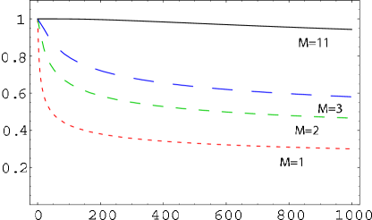
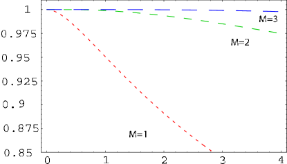
Figure 1: (Left) Plot of the ratio $\frac{R^{M-1}_{M}(Q^{2})}{\Phi_{Toy}(Q^{2})}$ as a function of $Q^{2}$, for $M=1,2,3$ and $M=11$. Notice the large values of $Q^{2}$ considered. (Right) Close-up of the same curves with $M=1,2,3$ in the low-$Q^{2}$ region.

$$\Phi_{Toy}(Q^{2})=\sum_{n=1}^{\infty}\frac{1}{n(Q^{2}+n)}\ ,$$ (16)

as a very simple toy model for the once-subtracted vacuum polarization (7) in the large-Nc limit. Obviously its spectrum consists of masses located at $M^{2}_{n}=1,2,3,...$, and one may use the mass of the lowest resonance as the unit of energy. An exact result for $\Phi_{Toy}(Q^{2})$ can be readily obtained as

$$\Phi_{Toy}(Q^{2})=\frac{1}{Q^{2}}\Big{\{}\psi(Q^{2}+1)+\gamma\Big{\}}$$ (17)

where the function $\psi(Q^{2}+1)$ is the Digamma function, defined as

$$\psi(z)=\frac{d}{dz}\log\Gamma(z)\ ,$$ (18)

with $\Gamma(z)$ the Euler Gamma function and $\gamma\simeq 0.577216$ being the Euler-Mascheroni constant. The function $\Phi_{Toy}(Q^{2})$ has the “chiral” expansion

$$\Phi_{Toy}(Q^{2})\approx\sum_{p=0}^{\infty}(-1)^{p}\zeta(p+2)\ Q^{2p}\ ,$$ (19)

where $\zeta(p+2)=\sum_{n=1}^{\infty}n^{-p-2}$ is the Riemann’s $\zeta$ function. On the other hand, the large $Q^{2}$ expansion is given by ($|\arg Q^{2}|<\pi$)

$$\Phi_{Toy}(Q^{2})\approx\frac{\gamma+\log Q^{2}}{Q^{2}}+\frac{1}{2Q^{4}}-\sum_{p=1}^{\infty}\frac{B_{2p}}{2p\ Q^{4p+2}}\ ,$$ (20)

where $B_{2p}=(-1)^{p+1}\frac{2(2p)!}{(2\pi)^{2p}}\ \zeta(2p)$ are the Bernoulli numbers for $p=1,2,3,...$.

While the chiral expansion has a finite radius of convergence $|Q^{2}|<1$, the large $Q^{2}$ expansion has zero radius of convergence (i.e. it is asymptotic) due to the factorial growth of the Bernoulli numbers. Notice also the presence of the $\log Q^{2}$ behavior in (20). Even so, Fig. 1 shows how the Pade Approximants $R^{M-1}_{M}$ are able to reproduce the full function at any finite value of $Q^{2}$. Notice that no step function simulating a perturbative “continuum” is needed [11]. The fact that they approach the true function from below is also well-known [4].

As to the prediction for the resonance masses, Table 1 shows the position of the poles of the given Pades and compares them to the true values for the masses. As anticipated before, the prediction for the masses gets worse the heavier the resonance, for a given Pade. The prediction for a low resonance, however, is certainly reasonable even for a low-order Pade and becomes much better as the order of the Pade increases.

	$R^{0}_{1}$	$R^{1}_{2}$	$R^{2}_{3}$	$R^{3}_{4}$	$R^{4}_{5}$	$R^{5}_{6}$
$M_{1}^{2}=1$	1.3684	1.0228	1.0010	1.0000	1.	1.
$M_{2}^{2}=2$		4.3711	2.2967	2.0409	2.0038	2.0002
$M_{3}^{2}=3$			10.1201	4.1755	3.2698	3.0526
$M_{4}^{2}=4$				19.5578	6.9160	4.8688

Table 1: Squared masses of the resonances obtained as poles of the corresponding Pade. For comparison, the true squared masses are also shown on the leftmost column.

In conclusion, Pade Approximants, when properly used, may turn out to be very useful tools for studying large-$N_{c}$ QCD. We have exemplified this in the case of the vacuum polarization because, having a positive spectral function, it happens to be a Stieltjes function, to which a known convergence theorem applies. But this case is not unique. Similar results will also apply to other correlators with positive spectral functions. Apart from this, it would certainly be most interesting to find out under which conditions Pade Approximants converge in more general situations when the spectral function is not positive definite.

The so-called two-point Pades also seem to be very promising, as they are able to connect the Operator Product and Chiral expansions[9]. However, to our knowledge, the consequences of their convergence properties for a QCD Green’s function have not yet been analyzed. It is clearly tempting to speculate about the possibility that they may be linked to theories with extra dimensions[12].

Acknowledgements

I am grateful to E. de Rafael for encouragement and numerous discussions, to F.J. Yndurain for correspondence and to M. Golterman for a critical reading of the manuscript. Finally, I would also like to thank P. Gonzalez-Vera for very useful conversations about Pades. This work has been supported by CICYT-FEDER-FPA2005-02211, SGR2005-00916 and by TMR, EC-Contract No. HPRN-CT-2002-00311 (EURIDICE).

References

- [1] G. ’t Hooft, Nucl. Phys. B 72 (1974) 461, Nucl. Phys. B 75 (1974) 461; E. Witten, Nucl. Phys. B 160 (1979) 57.
- [2] G.A. Baker and P. Graves-Morris, Pade Approximants, Encyclopedia of Mathematics and its Applications, Cambridge Univ. Press 1996. Section 5.4, Theorem 5.4.2.
- [3] See, e.g., J. Gasser and H. Leutwyler, Nucl. Phys. B 250 (1985) 465.
- [4] C. Bender and S. Orszag, Advanced Mathematical Methods for Scientists and Engineers I: asymptotic methods and perturbation theory, Springer 1999, section 8.6
- [5] G.A. Baker and P. Graves-Morris, Ref. [2]. Section 5.2, Theorem 5.2.1.
- [6] See, e.g., G. Ecker, J. Gasser, A. Pich and E. de Rafael, Nucl. Phys. B 321 (1989) 311; J. F. Donoghue, C. Ramirez and G. Valencia, Phys. Rev. D 39 (1989) 1947; S. Peris, M. Perrottet and E. de Rafael, JHEP 9805 (1998) 011 [arXiv:hep-ph/9805442].
- [7] G.A. Baker, Essentials of Pade Approximants, Academic Press 1975. Chapter 16, Theorem 16.2; see also, G.A. Baker and P. Graves-Morris, Ref.[2], Section 5.4, Theorem 5.4.4.
- [8] G.A. Baker and P. Graves-Morris, Ref.[2], Chapter 7.
- [9] G. Ecker, J. Gasser, H. Leutwyler, A. Pich and E. de Rafael, Phys. Lett. B 223 (1989) 425; M. Knecht and E. de Rafael, Phys. Lett. B 424 (1998) 335 [arXiv:hep-ph/9712457]; M. Knecht, S. Peris and E. de Rafael, Phys. Lett. B 443 (1998) 255 [arXiv:hep-ph/9809594]; E. de Rafael, Nucl. Phys. Proc. Suppl. 119 (2003) 71 [arXiv:hep-ph/0210317]; S. Peris, arXiv:hep-ph/0204181; A. Pich, Int. J. Mod. Phys. A 20 (2005) 1613 [arXiv:hep-ph/0410322].
- [10] B. Blok, M. A. Shifman and D. X. Zhang, Phys. Rev. D 57, 2691 (1998) [Erratum-ibid. D 59, 019901 (1999)] [arXiv:hep-ph/9709333].
- [11] See, e.g., M. Golterman, S. Peris, B. Phily and E. de Rafael, JHEP 0201 (2002) 024 [arXiv:hep-ph/0112042].
- [12] J. Erlich, G. D. Kribs and I. Low, arXiv:hep-th/0602110; J. Hirn and V. Sanz, JHEP 0512 (2005) 030 [arXiv:hep-ph/0507049]; L. Da Rold and A. Pomarol, Nucl. Phys. B 721 (2005) 79 [arXiv:hep-ph/0501218].