UCB-PTH-06/04

LBNL-59894

Improved Naturalness with a Heavy Higgs:
An Alternative Road to LHC Physics
Riccardo Barbieri^a, Lawrence J. Hall^b and Vyacheslav S. Rychkov^a
a Scuola Normale Superiore and INFN, Piazza dei Cavalieri 7, I-56126 Pisa, Italy

^b Department of Physics, University of California, Berkeley, and
Theoretical Physics Group, LBNL, Berkeley, CA 94720, USA

1 Introduction

Unification, likely supersymmetric, as developed in the seventies and eighties, is the most appealing and coherent picture that we have for physics beyond the Standard Model. Clear experimental evidence for it would represent a major breakthrough in physics and could orient the search for further informative signals. Yet the current situation is ambiguous. From the experimental viewpoint, on the positive side one has the unification of gauge couplings and, with less numerical significance, the size of the neutrino masses. On the negative side, however, one must consider the failure to find any supersymmetric particle, any non-SM effect in flavour physics, any evidence of proton decay, or, finally, a light Higgs boson. While there are many explanations for the absence of these signals so far, and searches for these phenomena should and will continue, we find it justified to consider possible alternative roads for physics beyond the SM. Especially, although not only, in these respects, the Large Hadron Collider should play a crucial role. This is the general background behind this work.

Our expectations for the LHC are based on two observations: 1) the Higgs mass gets quadratically divergent contributions, the dominant one being due to virtual top quarks, which become comparable to the physical mass for the cutoff $\Lambda_{t}\lesssim 3.5\;m_{h},$ and need to be cancelled by new physics to avoid unnatural fine-tuning. 2) ElectroWeak Precision Tests (EWPT) indicate that the SM Higgs is light, $m_{h}<186$ GeV at 95% CL [1], with a central value considerably below the lower bound of 114 GeV from direct searches. From 1) and 2) the standard view emerges, that the divergence-cancelling physics, whatever it is (supersymmetry, Little Higgs, …) should be accessible at the LHC.

In this paper we consider the alternative possibility that the Higgs is heavy, say $500$ GeV. In this case, the above conclusion does not apply, since the naturalness cutoff from 1) is now raised to $\sim 1.5$ TeV. Instead of focussing on the new physics which cancels the top quark divergence (squarks, vector quarks, …), we must consider the modified electroweak theory below $\Lambda_{t}$, that allows the heavy Higgs to pass the EWPT. Admittedly, to guess which physics may render a Heavy Higgs compatible with the EWPT is not easy. Some examples exist in the literature, starting from the work of Einhorn, Jones and Veltman[2] and recently reviewed by Peskin and Wells [3]. We postpone a few comments on this until Section 4. Here we argue that the most obvious way to do this, while keeping both naturalness and perturbativity, may reside in introducing an Inert Doublet (ID) scalar, i.e. a second Higgs without a vev or couplings to matter.

In the ID Model (IDM), the spectrum of the scalars, other than the true Higgs, of mass $m_{h}$, consists of a charged state, of mass $m_{H}$, and of two neutral states, of mass $m_{\text{L}}$ (L for lightest) and $m_{\text{NL}}$ (NL for next-to-lightest). The relation between these masses imposed by the EWPT is fully analogous to the one that relates the Higgs mass and the Z mass in the SM. In the entire perturbative regime of the IDM, we find that the range of the radiative correction effects has a large overlap with the corrections required to fit the precision data. We claim therefore that these data do not prefer the light Higgs of the SM over the Heavy Higgs of the IDM. On the other hand, in the IDM it is possible to raise the naturalness cut-off to about $1.5$ TeV without fine tunings. Other than consequences for the LHC mentioned above, this certainly ameliorates the problem posed by the “LEP paradox”[4], reducing by one order of magnitude the fine tuning apparently needed to fix it. Indeed, this improvement in naturalness is a major motivation for raising the Higgs boson mass, and occurs more readily than in 2 Higgs doublet models with a light Higgs [5], and more simply than in “Little Higgs” models. Furthermore, preliminary results from the TeVatron indicate a somewhat lighter top quark, strengthening the upper bound on the SM Higgs mass, and weakening the improved naturalness of the 2 Higgs doublet model with a light Higgs.

In most 2 Higgs doublet models a parity symmetry is introduced to ensure that Higgs exchange does not give too large flavour changing amplitudes. In the IDM the parity acts only on the inert doublet, and ensures that the doublet is inert. Unlike conventional 2 Higgs doublet models, the parity is not spontaneously broken by doublet vevs, and hence the Lightest Inert Particle, or LIP, is stable. In much of the parameter space the LIP contributes only a small fraction to the Dark Matter of the universe. But if there is a mild degree of cancellation in the LIP mass, so that it is in the range of 70 GeV, all DM can be accounted for by a neutral inert Higgs boson.

In Section 2 we set the stage by revisiting the SM with a heavy Higgs, paying special attention to the improved naturalness, the triviality bound on the Higgs mass, and to its incompatibility with EWPT constraints. In Section 3 we present the IDM, discussing in detail all the analogous constraints. In the same section we give a first description of the LHC signals of the IDM and we discuss the properties of the LIP as a Dark Matter candidate. In Section 4 we make a few comments on alternative models to render a heavy Higgs compatible with the EWPT. Summary and Conclusions are given in Section 5.

2 Standard Model with a Heavy Higgs

2.1 Improved naturalness

The SM is unnatural as a fundamental theory: the quadratic divergence of the Higgs mass makes the electroweak scale highly sensitive to the UV cutoff. Presumably, this quadratic divergence should be cancelled in the theory that extends the SM to higher energy scales. Two known mechanisms for accomplishing this are supersymmetry and realizing the Higgs as a pseudo-Goldstone boson. Searching for such mechanisms amounts to what we might call the qualitative use of the naturalness principle. However, the principle has also its other, quantitative side. Namely, it can be used to predict the energy scale by which the divergence-cancelling physics is expected to appear. Such a prediction follows from comparing the size of the one-loop quadratic divergence to the physical mass.

The quadratic divergence is given by ($v=174$ GeV)

$$\delta m_{h}^{2}=\alpha_{t}\Lambda_{t}^{2}+\alpha_{g}\Lambda_{g}^{2}+\alpha_{h}\Lambda_{h}^{2}$$ (1)

where

$$\alpha_{t}=\frac{3m_{t}^{2}}{4\pi^{2}v^{2}},\;\;\alpha_{g}=-\frac{6m_{W}^{2}+3m_{Z}^{2}}{16\pi^{2}v^{2}},\;\;\alpha_{h}=-\frac{3m_{h}^{2}}{16\pi^{2}v^{2}}$$ (2)

and $\Lambda_{i}$ are the cutoffs on the momenta of the virtual top quarks, gauge bosons, and the Higgs itself. We keep these cutoffs separate, because generally there is no reason to expect that the physics cancelling all three divergences will appear at exactly the same scale. In a more fundamental theory, the various $\Lambda_{i}$ may be correlated, but if we do not specify the theory which extends the SM and cancels the quadratic divergences, the relative weight of the various terms in (1) cannot be determined.

Knowing (1), we can compute the sensitivity of the Higgs mass to the scale $\Lambda_{i}$ by the formula

$$D_{i}(m_{h})\equiv\left|\frac{\partial\log m_{h}^{2}}{\partial\log\Lambda_{i}^{2}}\right|\,=\frac{|\alpha_{i}|\Lambda_{i}^{2}}{m_{h}^{2}}.$$ (3)

The meaning of this quantity is that if $D_{i}>1$, the theory needs fine-tuning of 1 part in $D_{i}$. The no fine-tuning condition $D_{i}\approx 1$ is equivalent to demanding that quadratic contributions in (1) (taken separately) do not exceed the physical mass squared. Using precise values of $\alpha_{i}$ given in (1), we obtain three no fine-tuning scales (for $D_{i}>1$ these scales should be multiplied by $\sqrt{D_{i}}$):

$$\Lambda_{t} \approx 3.5\,m_{h}$$

$$\Lambda_{g} \approx 9\,m_{h}>\Lambda_{t}$$ (4)

$$\Lambda_{h} \approx 1.3\text{ TeV}.$$

These equations are the quantitative outcome of the naturalness analysis—they bound the expected scale of the divergence-cancelling physics. Not surprisingly, the precise value of this scale crucially depends on the assumed value of the Higgs mass. The prevalent assumption nowadays is that the Higgs is light, with $m_{h}$ close to the $114$ GeV limit from the direct searches, so that the low value of $\Lambda_{t}$ makes us reasonably sure that at least the physics cancelling the virtual top divergence should be seen at the LHC.

But what if the Higgs is heavy, say $m_{h}\gtrsim 400$ GeV? The scale $\Lambda_{t}$ is raised above 1.4 TeV (“improved naturalness”), and since $\Lambda_{h}$ is also rather large, we can no longer be certain that the physics cancelling these divergences will be observable at the LHC. While $\Lambda_{i}$ only provide upper bounds on the scale of the cancellation physics, in the absence of supersymmetry, given the LEP paradox, it is likely that these bounds are saturated. What will the LHC see in this case? This is the question we would like to address.

2.2 Perturbativity, or how heavy is heavy?

How high up in $m_{h}$ can one go? As the Higgs mass is increased so the quartic scalar interaction becomes stronger, and the maximum scale at which perturbation theory is useful, $\Lambda_{P}$, is decreased. Our aim is to have a natural theory up to energies of 1.5 TeV, hence we must require that $\Lambda_{P}>$ 1.5 TeV, placing an upper bound on the Higgs mass. If this requirement is fulfilled, we can reasonably assume that the divergence-cancelling physics, which is expected to appear just around that scale will also be able to stop the growth of the Higgs quartic coupling and prevent the Landau pole from appearing. The RG evolution of the Higgs quartic coupling is reviewed in Appendix A. The results of that discussion can be summarized in terms of two scales: the one-loop Landau pole scale $\Lambda_{L}$, and the perturbativity scale $\Lambda_{P}$ at which the quartic coupling grows by 30% from its value in the IR. The values of these two scales for $m_{h}=400,500,600$ GeV are given in Table 1. We see that in all cases $\Lambda_{P}$ is above 1.5 TeV, while $\Lambda_{L}$ is $5-30$ times higher. The conclusion is that all masses in the $400-600$ GeV range are suitable for the implementation of the improved naturalness idea.

$m_{h},$GeV	$\Lambda_{P},$TeV	$\Lambda_{L}$,TeV
400	2.4	80
500	1.8	16
600	1.6	7.5

Table 1: Heavy Higgs perturbativity scale $\Lambda_{P}$ and Landau pole $\Lambda_{L}$.

2.3 ElectroWeak Precision Tests

At this point the reader should ask: but what about the EWPT, which predict that the Higgs is light? The answer of course is that this ‘prediction’ is true only in the absence of new physics, which may contribute to the EWPT observables, but has nothing to do with cancelling the quadratic divergences of the Higgs mass. Indeed, the Higgs mass influences the EWPT via the logarithmic contributions to $T$ and $S$:

$$T \approx-\frac{3}{8\pi c^{2}}\ln\frac{m_{h}}{m_{Z}}$$ (5)

$$S \approx\frac{1}{6\pi}\ln\frac{m_{h}}{m_{Z}}.$$ (6)

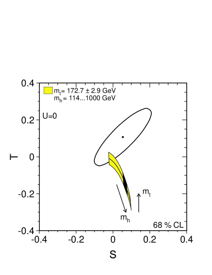
For large $m_{h}$ these contributions violate experimental constraints (see Fig. 1). Assuming that no new physics influences the EWPT, one obtains $m_{h}=91_{-32}^{+45}$ GeV, with the upper bound $m_{h}<186$ GeV at 95% CL [1]. In particular $m_{h}=400$ GeV is excluded at 99.9% CL.

However, looking at Fig. 1 one immediately sees that the heavy Higgs can be consistent with the EWPT if there is new physics producing a compensating positive $\Delta T$. If at the same time the $\Delta S$ contribution of this new physics is not too large, a good fit could be obtained. For $m_{h}=400-600$ GeV (black band in Fig. 1) the needed compensating $\Delta T$ is

$$\Delta T\approx 0.25\pm 0.1,$$ (7)

which would bring us near the central point of the 68% CL ellipse (the uncertainty in this number is mostly due to the experimental error on $T$). Rather than making a careful fit, in this paper we will be content with this rough estimate.

Figure 1: (Adapted from [8].) Dependence of the $S,T$ parameters on the Higgs mass. The thick black band marks $m_{h}=400-600$ GeV.

Thus the answer to the question of what the LHC will see is: If the Higgs is heavy, there must be new physics producing a positive $\Delta T$, and it is this new physics that the LHC will study.

3 The Inert Doublet Model

In this section we will present what seems to us the most attractive realization of the improved naturalness idea. Some alternatives are described in Section 4.

3.1 The Model

We consider the most general two-Higgs doublet model that possesses the parity

$$H_{2}\rightarrow-H_{2}$$ (8)

with all other fields invariant. This parity imposes natural flavor conservation in the Higgs sector[9], implying that only $H_{1}$ couples to matter. The scalar potential is

$$V =\mu_{1}^{2}|H_{1}|^{2}+\mu_{2}^{2}|H_{2}|^{2}+\lambda_{1}|H_{1}|^{4}+\lambda_{2}|H_{2}|^{4}+\lambda_{3}|H_{1}|^{2}|H_{2}|^{2}$$

$$\quad+\lambda_{4}|H_{1}^{\dagger}H_{2}|^{2}+\frac{\lambda_{5}}{2}[(H_{1}^{\dagger}H_{2})^{2}+\text{h.c.}].$$ (9)

We assume that the parameters of this potential yield an asymmetric phase: $H_{1}$ acquires a vev but $H_{2}$ does not This is not the well-studied standard phase of the theory that has both vevs non-zero, and it cannot be obtained as the small $\tan\beta$ limit of the standard phase, which is a fine tuned limit. Rather, the asymmetric phase results in a parameter region of comparable size to the standard phase, depending essentially on the sign of $\mu_{2}^{2}$. The doublet $H_{1}$ is identified as essentially the SM Higgs doublet—it gets a vev and gives masses to $W,Z$ and fermions. On the other hand, $H_{2}$ does not couple to fermions and does not get a vev. We will call it the inert doublet, although of course it does have weak interactions and quartic interactions.

The scalar spectrum of the theory is obtained by expanding the potential around the minimum

$$H_{1}=(0,v),\quad H_{2}=(0,0).$$ (10)

The physical fields appear in the parametrizaton of the doublets as follows:

$$H_{1}=\left(\begin{array}[c]{c}\phi^{+}\\ v+(h+i\chi)/\sqrt{2}\end{array}\right),\qquad H_{2}=\left(\begin{array}[c]{c}H^{+}\\ (S+iA)/\sqrt{2}\end{array}\right).$$ (11)

Here the Goldstones $\phi^{+},\chi$ can be put to zero by choosing the unitary gauge; they are included for future reference. The usual Higgs boson is $h$, which we take to be heavy:

$$m_{h}\approx 400-600~{}\text{GeV\quad(}\lambda_{1}=m_{h}^{2}/4v^{2}\approx 2).$$ (12)

In addition, we have three “inert” particles—a charged scalar $H^{+}$ and two neutrals $S,A$ with masses:

$$m_{I}^{2} =\mu_{2}^{2}+\lambda_{I}v^{2},\quad I=\{H,S,A\}$$ (13)

$$\lambda_{H} =\lambda_{3}$$

$$\lambda_{S} =\lambda_{3}+\lambda_{4}+\lambda_{5}$$

$$\lambda_{A} =\lambda_{3}+\lambda_{4}-\lambda_{5}.$$

We assume that the potential (9) is bounded from below, which happens if and only if

$$\lambda_{1,2}>0;\qquad\lambda_{3},\lambda_{\text{L}}\equiv\lambda_{3}+\lambda_{4}-|\lambda_{5}|>-2(\lambda_{1}\lambda_{2})^{1/2}.$$ (14)

Under this assumption, the minimum (10) is stable and global, as long as all masses squared (13) are positive.

The way to visualize the parameter space of the 7 parameters of the potential (9) is as follows. These 7 parameters can be traded for the four physical scalar masses, $m_{h},m_{H},m_{A},m_{S}$, the vev $v$ (or the Z-mass) and the two quartic couplings, $\lambda_{2}$ and $\lambda_{3}$. The EWPT imply a relation between the 5 parameters with dimension of mass, analogous to the relation between $m_{h}$ and $m_{Z}$ in the SM. Since the inert parity, (8), is unbroken, the lightest inert particle (LIP) will be stable and will contribute to the Dark Matter density. It may in fact constitute all of the DM if the parameters have the right value, although the typical fraction is small. In any case, to avoid conflicting with the stringent limits on charged relics [11], we will always assume that the LIP is neutral. In the limit of Peccei-Quinn symmetry, $\lambda_{5}\rightarrow 0$, the neutral inert scalars $S$ and $A$ become degenerate. Direct detection of halo dark matter places a limit on this degeneracy [12], because the mass difference must be sufficient to kinematically suppress the scattering of galactic LIPs on nuclei via tree-level Z boson exchange.

Of the two dimensionless couplings, $\lambda_{2}$ only affects the self-interactions between the inert particles. It is difficult to even conceive how it could be measured. To avoid additional problems with perturbativity, we assume that it is quite small,

$$\lambda_{2}\lesssim 1\,.$$ (15)

On the contrary, $\lambda_{3}$ may affect some significant observables, like the width of $h$ (see Eq. (49)) and (if parameters take values to allow LIP DM) the interaction cross section of the DM with nuclei (see Eq. (37)).

Analogously to the SM case, in the next sub-sections we discuss constraints imposed on the IDM parameters by perturbativity, naturalness, and the EWPT, and we summarize the allowed regions of couplings in Section 3.5. In a large region of parameter space we will find that the heavy Higgs has naturalness and perturbativity properties very similar to the SM heavy Higgs described in section 2. The advantage of the IDM is that the mass splittings within the inert doublet allow a satisfactory $T$ parameter.

3.2 Perturbativity

Let us begin with perturbativity. The RG equations satisfied by the two-Higgs doublet model couplings are given in Appendix B. To determine the exact high-energy behavior, one would have to find precise initial conditions for all couplings, similarly to what we have done for the SM in Appendix A. Here we will be content with deriving some sufficient conditions for perturbativity. First let us look at $\lambda_{1}$, whose beta-function equation is

$$16\pi^{2}\frac{d\lambda_{1}}{d\log\Lambda}=24\lambda_{1}^{2}+2\lambda_{3}^{2}+2\lambda_{3}\lambda_{4}+\lambda_{4}^{2}+\lambda_{5}^{2}.$$ (16)

As we discussed in Section 2.2, the SM with a 500 GeV Higgs stays perturbative up to a reasonably high scale $\sim 1.8$ TeV. In order that this conclusion be preserved in our model, we will impose a requirement that the sum the of extra terms in the RHS of (16) not exceed 50% of the SM term $24\lambda_{1}^{2}$. Thus we get a constraint (see Eq. (12))

$$|2\lambda_{3}(\lambda_{3}+\lambda_{4})+\lambda_{4}^{2}+\lambda_{5}^{2}|\lesssim 50\text{ \ \ \ (perturbativity).}$$ (17)

How large can the couplings become consistent with this inequality? One possibility is that $|\lambda_{4}|$ becomes large, while $\lambda_{5}$ stays relatively small. In this case we must have $\lambda_{4}<0$ for the LIP to be neutral. This implies that $\lambda_{3}$ must also become large, $\lambda_{3}\gtrsim|\lambda_{4}|$, to ensure the vacuum stability (14) (remember that $\lambda_{2}$ is assumed to be small.) The critical region is when $\lambda_{3}\sim|\lambda_{4}|$ so that the first term in (17) vanishes. This way we get the bound

$$|\lambda_{4}|\lesssim\lambda_{3}\lesssim 7\quad(\lambda_{4}<0\text{, }\lambda_{5}\text{ small).}$$ (18)

The other possibility is that, on the contrary, it is $\lambda_{5}$ which becomes large, while $\lambda_{4}$ is small. In this case, the vacuum stability condition (14) implies $\lambda_{3}\gtrsim|\lambda_{5}|$, leading to a stricter bound

$$|\lambda_{5}|\lesssim\lambda_{3}\lesssim 4\text{\qquad(}\lambda_{4}\text{ small).}$$ (19)

As we will see in Section 3.4 below, it is only the first possibility that will lead to $\Delta T>0$, as needed to compensate for the heavy Higgs. However, for the time being we want to explore all possibilities so that we can understand the typical range of $\Delta T$ allowed in our model.

Finally, we have checked that, in the region allowed by the constraints (18) or (19), the evolution of the remaining couplings does not lead to any additional restrictions. Essentially this happens because we assume that $\lambda_{2}$ is sufficiently small and because $\lambda_{3,4,5}$ evolve slower than $\lambda_{1}$ due to the smaller RG coefficients.

3.3 Naturalness

Like the SM, the IDM is a natural effective theory only up to some cutoff, which is determined by the quadratic divergences in the dimensional parameters. For the IDM there are two mass parameters, $\mu_{1,2}^{2}$, and we must study naturalness for each separately, obtaining conditions that allow the theory to be natural for energies up to 1.5 TeV.

Since $\mu_{1}^{2}$ is linear in the Higgs mass squared, as in the SM case it is convenient to study the corrections to $m_{h}^{2}$. Introducing separate cutoffs for loops of virtual $H_{1}$ and $H_{2}$ particles, $\Lambda_{H_{1,2}}$, we find a result similar to (1)

$$\delta m_{h}^{2}=\alpha_{t}\Lambda_{t}^{2}+\alpha_{g}\Lambda_{g}^{2}+\alpha_{11}\Lambda_{H_{1}}^{2}+\alpha_{12}\Lambda_{H_{2}}^{2}$$ (20)

where

$$\alpha_{11}=-\frac{3\lambda_{1}}{4\pi^{2}},\;\;\alpha_{12}=-\frac{2\lambda_{3}+\lambda_{4}}{8\pi^{2}}$$ (21)

and $\alpha_{t,g}$ are as in (2). The first three terms lead to the bounds of (2.1), except that it is now $\Lambda_{H_{1}}$, rather than $\Lambda_{h}$, that is limited by 1.3 TeV. This last bound cannot be avoided without changing or cancelling the effect of the usual Higgs quartic, which the IDM does not do. This is why we content ourselves with a theory that is natural up to about 1.5 TeV. The scales $\Lambda_{t,g}$ are raised to 1.5 TeV or more by taking the Higgs mass heavier than 400 GeV. Requiring that the last term of (20) not exceed the physical Higgs mass squared gives the additional constraint

$$|2\lambda_{3}+\lambda_{4}|\lesssim 9.$$ (22)

The one-loop quadratic divergences to $\mu_{2}^{2}$ are

$$\delta\mu_{2}^{2}=-\frac{1}{2}\left(\alpha_{g}\Lambda_{g}^{2}+\alpha_{22}\Lambda_{H_{2}}^{2}+\alpha_{21}\Lambda_{H_{1}}^{2}\right)$$ (23)

where

$$\alpha_{22}=-\frac{3\lambda_{2}}{4\pi^{2}},\;\;\;\;\alpha_{21}=-\frac{2\lambda_{3}+\lambda_{4}}{8\pi^{2}}.$$ (24)

Requiring each of these three corrections to be smaller than the tree-level value, leads to the three naturalness constraints

$$\mu_{2}\gtrsim\left(1,\;2.5\sqrt{\lambda_{2}},\;\sqrt{|2\lambda_{3}+\lambda_{4}|}\right)120\,\mbox{GeV}$$ (25)

respectively.

We have required that our model is a natural effective field theory in the sense that the sensitivity of Lagrangian parameters to variations in the cutoff is small: $D_{i}(\mu_{1,2}^{2})\lesssim 1$. We do not attempt to impose the stronger condition that all observables have small such sensitivities. It may be that some observables are small because of cancelling contributions within the effective theory. For example, from (13) we see that a LIP mass $m_{\text{L}}\ll\mu_{2}$ requires a cancellation between $\mu_{2}^{2}$ and $\lambda_{3,4,5}v^{2}$ terms. Another example is the Z boson mass in the minimal supersymmetric standard model with a heavy top squark. While these cancellations should also be avoided, they differ from the cancellations at the cutoff that are required between tree and loop contributions to Lagrangian parameters. In particular they become acceptable if it is possible to measure sufficient quantities to demonstrate that such cancellations occur in the low energy theory. Given the expression (13) for the inert scalar masses, it is natural to expect that some inert scalars could be somewhat lighter than $\mu_{2}$, and some could be heavier. Since it is reasonable that the terms in (13) for the LIP do not all have the same sign, it is certainly natural for the LIP to be lighter than $\mu_{2}$. We consider $m_{\text{L}}$ to be natural if

$$m_{\text{L}}\gtrsim\frac{\mu_{2}}{2}.$$ (26)

3.4 ElectroWeak Precision Tests

Finally, let us evaluate the IDM from the EWPT viewpoint. The heavy Higgs contributions to $T$ is given in (6) and is to be compensated by the contribution from the inert doublet, which is computed in Appendix C to be

$$\Delta T =\frac{1}{32\pi^{2}\alpha v^{2}}[F(m_{H},m_{A})+F(m_{H,}m_{S})-F(m_{A},m_{S})],$$ (27)

$$F(m_{1},m_{2})=\frac{m_{1}^{2}+m_{2}^{2}}{2}-\frac{m_{1}^{2}m_{2}^{2}}{m_{1}^{2}-m_{2}^{2}}\ln\frac{m_{1}^{2}}{m_{2}^{2}}.$$ (28)

This contribution comes from the $\lambda_{4,5}$ terms in the potential, since these are the terms breaking the custodial symmetry. From (13), it is clear that the same terms are responsible for the mass splitting among the inert scalars. The function $F(m_{1},m_{2})$ is positive, symmetric, vanishes for $m_{1}=m_{2}$ and monotonically increases for $m_{1}\geq m_{2}$. Moreover, to high accuracy, 2$\ldots$5% for $1\leq m_{1}/m_{2}\leq 2\ldots 3$, we have

$$F(m_{1},m_{2})\approx\frac{2}{3}(m_{1}-m_{2})^{2}.$$ (29)

For our purposes it will always be sufficient to use this approximation, allowing (27) to be simplified

$$\Delta T\approx\frac{1}{24\pi^{2}\alpha v^{2}}(m_{H}-m_{A})(m_{H}-m_{S}).$$ (30)

Requiring this $\Delta T$ be in the range (7), we find a constraint on the spectrum

$$(m_{H}-m_{S})(m_{H}-m_{A})=M^{2},\qquad M=120_{-30}^{+20}\text{ GeV}\,.$$ (31)

Since the LIP is neutral, we see that $H$ should be heavier than both $S$ and $A$ to have $\Delta T>0$.

The contribution of the inert doublet to $S$ is also given in Appendix C, Eq. (65). It depends on the inert particle masses only logarithmically, and remains small ($|\Delta S|\lesssim 0.04$) for the whole range of parameters considered below. Thus its effect on the EWPT fit can be neglected.

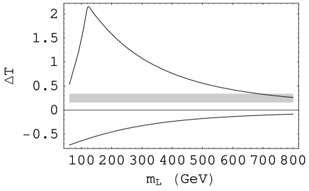
To evaluate the success of the IDM in compensating for the heavy Higgs, it is important to know the typical range of $\Delta T$ allowed by naturalness and perturbativity. The relevant constraints on the parameters are (14,15,18,19,25,26). The resulting $\Delta T$ range is shown as a function of $m_{\text{L}}$ in Fig. 2. For $m_{\text{L}}\gtrsim 300$ GeV the perturbativity constraints (18,19) are more restrictive, while for smaller $m_{\text{L}}$ the naturalness constraints become crucial. The maximal $\Delta T>0$ occurs when $\lambda_{4}$ is large and negative, while $\lambda_{5}$ remains small. The maximal $\Delta T<0$ is achieved in the opposite regime of $\lambda_{4}$ small, $\lambda_{5}$ large. We see that $\Delta T$ is predominantly positive and is of the typical size needed to compensate for the heavy Higgs in a large region of the parameter space. We conclude that the success of our model is not accidental. If it had turned out that the needed $\Delta T$ was much smaller than the typical value, then we would have imposed approximate custodial symmetry on the potential. But we see that little, if any, suppression from custodial symmetry is needed in most of the range of $m_{\text{L}}$.

Figure 2: The maximal and minimal $\Delta T$ allowed by naturalness and perturbativity as a function of $m_{L}$. The horizontal grey band marks the range needed to compensate for the heavy Higgs.

3.5 Summary of constraints on the spectrum and couplings

Preparing for the discussion of signals, let us describe the region of parameter space that leads to a natural, perturbative effective theory up to 1.5 TeV and that satisfies the EWPT constraint (31). It is convenient to use a parametrization in terms of the masses of the two neutral inert particles, $m_{\text{L}}$ for the lightest and $m_{\text{NL}}$ for the next-to-lightest. We consider the general case when $\Delta m=m_{\text{NL}}-m_{\text{L}}$ can be sizeable. The charged scalar is always heavier than both neutrals, and using (31), the second splitting can be expressed in terms of $\Delta m$ and $M$

$$m_{H}-m_{\text{NL}}=\sqrt{M^{2}+\frac{(\Delta m)^{2}}{4}}-\frac{\Delta m}{2}$$ (32)

and is shown in Fig. 3 for the range $M=120^{+20}_{-30}$ GeV.

Figure 3: The relation between the first and the second spacing in the inert particle spectrum following from the EWPT constraint (31).

The couplings $\lambda_{4,5}$ can be also expressed via $m_{\text{L}},m_{\text{NL}}$ using (32) and (13), giving

$$\lambda_{4} =-\frac{1}{v^{2}}\left(M^{2}+(m_{\text{L}}+m_{\text{NL}})\sqrt{M^{2}+\frac{(\Delta m)^{2}}{4}}\right)<0$$ (33)

$$|\lambda_{5}| =\frac{m_{\text{NL}}^{2}-m_{\text{L}}^{2}}{2v^{2}}<|\lambda_{4}|.$$ (34)

The sign of $\lambda_{5}$ depends on whether it is the scalar $S$ or the pseudoscalar $A$ which is the heavier.

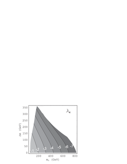
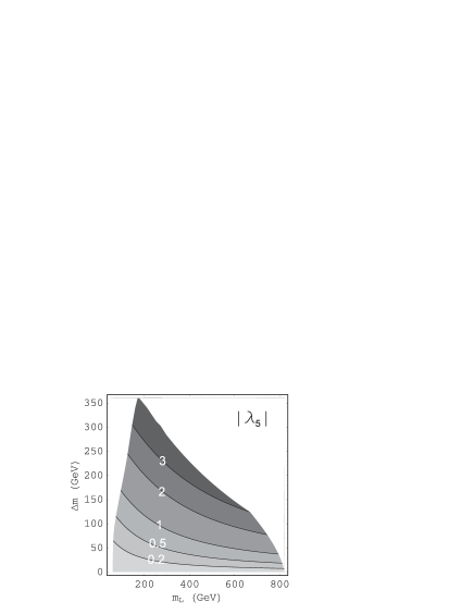
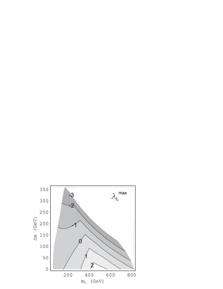
The coupling $\lambda_{3}$ (or $\lambda_{\text{L}}\equiv\lambda_{3}+\lambda_{4}-|\lambda_{5}|$) is the only free parameter; it should be chosen in agreement with the perturbativity (15,18), naturalness (22,25,26), and vacuum stability (14) constraints. These constraints can be used to derive a range of allowed values:

$$\lambda_{\text{L}}^{\min}(m_{\text{L}})\lesssim\lambda_{\text{L}}\lesssim\lambda_{\text{L}}^{\max}(m_{\text{L}},\Delta m)$$ (35)

The (iso)plots of $\lambda_{4,5}$ $\lambda_{\text{L}}^{\min},\lambda_{\text{L}}^{\max}$ are given in Fig. 4,5. The white region has $\lambda_{\text{L}}^{\min}>\lambda_{\text{L}}^{\max}$ or $|\lambda_{4}|>7$ and is disfavored by naturalness and/or perturbativity.

Thus we conclude that the IDM is a fully natural effective field theory up to 1.5 TeV for a large region of parameter space where the Higgs is heavy and EWPT are satisfied. Of the 7 parameters in the potential, $\mu_{1}^{2}$ and $\lambda_{1}$ can be traded for $v$ and $m_{h}$, while $\mu_{2}^{2}$ and $\lambda_{3,4,5}$ can be traded for $m_{\text{L}},m_{\text{NL}},m_{H},$ and $\lambda_{\text{L}}$. EWPT constrains $m_{\text{H}}-m_{\text{NL}}$ as shown in Figure 3. The allowed ranges of $m_{\text{L}}$ and $\Delta m$ are shown shaded in Figure 4, and the allowed range of $\lambda_{\text{L}}$ is shown in Figure 5. From perturbativity, $\lambda_{2}\lesssim 1$.

Figure 4: $\lambda_{4,5}$ in the allowed region as functions of $m,\Delta m$ computed from (33), (34) with $M=120$ GeV.

Figure 5: $\lambda_{\text{L}}^{\min}$ and $\lambda_{\text{L}}^{\max}$  for $M=120$ GeV. Notice that $\lambda_{\text{L}}^{\min}$ depends only on $m_{\text{L}}$ and is constant for $m_{\text{L}}\gtrsim 180$ GeV.

3.6 Dark Matter

We now begin the discussion of signals. As we already mentioned, the LIP is stable, and thus provides a cold Dark Matter candidate. Here we will estimate its relic abundance and discuss prospects for direct detection.

3.6.1 Relic abundance

Case I: $m_{\text{L}}\gtrsim m_{W}$

This case is of significant interest, since it includes most of the region of parameter space preferred by naturalness. The dominant annihilation process is into gauge bosons, with s-wave cross section $\sigma_{\text{ann}}v_{\text{rel}}\sim 130$ pb for $m_{\text{L}}\sim m_{W}$, decreasing to $\sim 10$ pb for $m_{\text{L}}\sim 400$ GeV (see Appendix D.1). A particular feature of our model is that the cross section does not decrease further due to the contribution of the longitudinal final states. Using the standard formalism [13], we find the relic density $\Omega_{\text{DM}}h^{2}\lesssim 0.02$ in the whole range of $m_{\text{L}}$, decreasing to $0.002$ for $m_{\text{L}}\sim m_{W}$. This number can be trusted as an order of magnitude estimate all the way down to the $WW$ production threshold. Since this is much lower than the observed $\Omega_{\text{DM}}h^{2}\sim 0.1$, we conclude that in this region of parameter space the LIP provides only a sub-dominant component of the Dark Matter.

Case II: $m_{\text{L}}<m_{W}$

Let us focus on the region $m_{\text{L}}=(60\text{--}80)$ GeV. While some cancellations in (13) for the LIP mass are required, they are mild and satisfy (26).

As the temperature of the early universe falls well below $m_{L}$, thermal equilibrium is maintained via p-wave suppressed coannihilations of $S$ and $A$ into fermions, and the relic abundance critically depends on $\Delta m$. In appendix D.2, we find the thermally averaged cross section, for $\Delta m\ll T_{\text{f}}\sim m/25$, to be $\langle\sigma_{\text{coann}}v_{\text{rel}}\rangle\sim(60\text{--}15)$ pb, for $m_{\text{L}}=(60\text{--}80)$ GeV. This leads to the relic density $\Omega_{\text{DM}}h^{2}\approx(0.5\text{--}2.5)\times 10^{-2}$, still below the observed value. On the other hand, for $\Delta m\gtrsim T_{\text{f}}$ the density of the heavier component is thermally suppressed and the coannihilation rate decreases. A formalism to compute the relic abundance in such non-standard situations was developed in [14]. However, the final result can be predicted without making difficult calculations. Roughly, the resulting relic density will be a factor $\sim(1/2)\exp(\Delta m/T_{\text{f}})$ larger than in the unsplit case, where $1/2$ takes into account that only the lighter component now contributes to the final abundancy. This way we deduce that $\Delta m_{\text{naive}}\approx 8$ GeV should be enough to yield the observed DM density.

The above naive argument can be expected to work at least for $m_{\text{L}}\lesssim m_{W}-3T_{\text{f}}/2\approx 75$ GeV; for higher masses the annihilation into $WW$ becomes thermally allowed and suppresses the relic abundance. Using the above-mentioned formalism of [14], these numbers can be confirmed (see Fig. 6). In particular we find $\Delta m\approx(8\mbox{--}9)$ GeV for $m_{\text{L}}=(60\mbox{--}73)$ GeV,  increasing to $12$ GeV for $m_{\text{L}}=75$ GeV, while for $m_{\text{L}}\geq 76$ GeV no splitting gives the observed DM density.

Figure 6: The mass splitting between the neutral inert particles needed to get the observed DM abundance below the WW threshold (obtained using the formalism from [14]). For $m_{\text{L}}\geq 76$ GeV no splitting works.

3.6.2 Direct detection

The $S$ and $A$ have a vector-like interaction with the $Z$-boson, which produces a spin-independent elastic cross section on a nucleus $\mathcal{N}$

$$\sigma_{Z}(\text{L\thinspace}\mathcal{N}\rightarrow\text{L}\,\mathcal{N})=\frac{G^{2}_{\text{F}}m_{r}^{2}}{2\pi}[N-(1-4s_{\text{w}}^{2})Z]^{2}\text{,}$$ (36)

where $N$ and $Z$ are the numbers of neutrons and protons in the nucleus, and $m_{r}=m_{L}m_{\mathcal{N}}/(m_{L}+m_{\mathcal{N}})$ is the reduced mass. The resulting per nucleon cross section is 8-9 orders of magnitude above the existing limits [12]. Thus we have to assume that there exists a non-zero splitting between $S$ and $A$ larger than the kinetic energy of DM in our galactic halo, so that the process (36) is forbidden kinematically. This constraint must be imposed whether $m_{\text{L}}$ is above or below $m_{W}$—even though the LIP relic density for $m_{\text{L}}\gtrsim m_{W}$ is small, it is still too large to allow elastic scattering from nuclei via tree-level $Z$-exchange.

Tree-level $h$ exchange produces a spin-independent cross section [15]:

$$\sigma_{h}(\text{L\thinspace}\mathcal{N}\rightarrow\text{L\thinspace}\mathcal{N})=\frac{m_{r}^{2}}{4\pi}\left(\frac{\lambda_{\text{L}}}{m_{\text{L}}m_{h}^{2}}\right)^{2}f^{2}m_{\mathcal{N}}^{2}\text{,}$$ (37)

where $f\sim 0.3$ is the usual nucleonic matrix element:

$$\langle\mathcal{N}|\sum m_{q}q\bar{q}|\mathcal{N}\rangle=fm_{\mathcal{N}}\langle\mathcal{N}|\mathcal{N}\rangle.$$ (38)

Another allowed process, the exchange of two gauge bosons at one loop, gives an effective coupling to nucleons similar to the tree-level $h$ exchange (see [16] for a recent discussion). For $m_{\text{NL}}-m_{\text{L}}\ll m_{Z}$, the resulting spin-independent cross section is independent of $m_{\text{L }}$and can be estimated as

$$\sigma_{\text{VV}}(\text{L\thinspace}\mathcal{N}\rightarrow\text{L\thinspace}\mathcal{N})\sim\frac{m_{r}^{2}}{4\pi}\left[\frac{(g/2c_{\text{w}})^{4}}{16\pi^{2}m_{Z}^{3}}\right]^{2}f^{2}m_{\mathcal{N}}^{2},$$ (39)

while for larger splittings a cross section estimate can be obtained by replacing $m_{Z}^{3}$ in the amplitude by $m_{\text{L}}m_{Z}^{2}$.

The numerical value of the cross-section (37) for scattering from a proton is

$$\sigma_{h}(\text{L}p\rightarrow\text{L}p)\approx 2\times 10^{-9}\;\mbox{pb}\;\left(\frac{\lambda_{L}}{0.5}\right)^{2}\left(\frac{70\,\mbox{GeV}}{m_{L}}\right)^{2}\left(\frac{500\,\mbox{GeV}}{m_{h}}\right)^{4}.$$ (40)

Our mass choices follow because the relic LIP abundance can yield the observed DM for $m_{L}\approx$ 60–75 GeV, and the cutoff scales of the theory are quite high if the Higgs is heavy, $m_{h}\approx$ 400–600 GeV. These ranges for $m_{L}$ and $m_{h}$ do lot lead to a wide variation of $\sigma_{h}$. The largest uncertainty in $\sigma_{h}$ arises from $|\lambda_{L}|=(\mu_{2}^{2}-m_{L}^{2})/v^{2}$. From (25) and (26) naturalness suggests that, for this interesting case of a light LIP, $\mu_{2}$ should be close to its lowest natural value of 120 GeV, giving $|\lambda_{L}|\approx 0.5$, the value used in (40). In this region of parameter space, the cross section as estimated in (39) is typically an order of magnitude smaller. Thus we expect a signal two orders of magnitude below the present limit from Ge detectors [12] and within the sensitivity of experiments currently under study.

Finally, for $m_{\text{L}}\gtrsim m_{W}$ we are penalized by a smaller relic density and by the $m_{\text{L}}^{-2}$ decrease of (37). The prospects for near-future direct detection in this case are dim.

3.7 Collider signals

3.7.1 Production and decay of the inert particles

The inert particles can be only pair-produced. If $m_{\text{L}}\approx 70$ GeV and $\Delta m$ is small, as preferred in the DM region, $SA$ pairs were produced at LEP2. Assuming $\Delta m\ll m_{\text{L}}$, the production cross section is

$$\sigma(e^{+}e^{-}\rightarrow SA)=\left(\frac{g}{2c_{\text{w}}}\right)^{4}\left(\frac{1}{2}-2s_{\text{w}}^{2}+4s_{\text{w}}^{4}\right)\frac{1}{48\pi s}\frac{[1-4m^{2}/s]^{3/2}}{[1-m_{Z}^{2}/s]^{2}}\approx 0.2\text{ pb}$$ (41)

for $\sqrt{s}=200$ GeV. The heavier state, which for definiteness we take to be $A$, decays into the lighter plus $Z^{\ast}$. The resulting dilepton events with missing energy were looked for in the context of searches for the lightest superpartner. For small mass differences, $\Delta m\lesssim 10$ GeV, the production cross section (41) is below the existing limits set by the separate LEP collaborations [17]. However, our signal is close to these limits, so that a combined reanalysis of the old data may be useful.

At the LHC pairs of inert particles will be produced by

$$pp \rightarrow W^{\ast}\rightarrow HA\text{ or }HS$$ (42)

$$pp \rightarrow Z^{\ast}(\gamma^{\ast})\rightarrow SA\text{ or }H^{+}H^{-}$$ (43)

and will decay by

$$H \rightarrow AW\text{ or }SW$$ (44)

$$A \rightarrow SZ^{(\ast)}.$$ (45)

One can thus imagine various decay chains, with final states containing several leptons, jets and missing transverse energy.

For the purposes of detection, the events with charged leptons in the final state seem most promising. In the region preferred by DM, the decay (45) gives events having the lepton pair invariant mass sharply peaked at low values, with a cutoff determined by $\Delta m\lesssim 10$ GeV. An extra charged lepton coming from $H$ via (44) is likely needed to help discriminate against the SM background. We have estimated the number of the inert particle pair production events at the LHC with at least 3 charged leptons in the final states using PYTHIA [18]. In the region preferred by DM, the process (42) has cross section $\sim 0.25$ pb, and a branching ratio (BR) into at least 3 electrons or muons of $\sim 1.5\%$. The effective cross section of signal events with 3 charged leptons is thus estimated as

$$\sigma_{\text{signal}}\approx 3.5\text{ fb}$$ (46)

The $H^{+}H^{-}$ pair production has cross section about an order of magnitude smaller because of the higher mass. The dominant irreducible background is likely to be the $WZ$ pair production with the $W$ decaying into electrons or muons and the $Z$ into $\tau$-pairs, with the $\tau$’s also decaying into electrons or muons. We assume that the background from direct decays of the $Z$ into electrons or muons can be easily eliminated. In this case we estimate the effective cross section of background events as

$$\sigma_{\text{bg}}\approx 20\text{ fb}$$ (47)

An integrated luminosity $\mathcal{L}\sim 30$ fb^-1 might therefore allow a detection of the signal. It would be very interesting to perform a complete study going beyond these rough estimates. We are aware of the problems that might arise from other sources of backgrounds, like the production of $t\bar{t}$ pairs, which has been studied in an analogous supersymmetric context [19], or the $W\gamma^{\ast}$ production.

3.7.2 The Higgs width

The existence of the new states may be inferred indirectly from the increase of the width of the usual Higgs. The new decay channels are

$$h\rightarrow SS,AA,H^{+}H^{-}$$ (48)

and the resulting increase in the width of $h$ is

$$\Delta\Gamma=\frac{v^{2}}{16\pi m_{h}}\left[\lambda_{S}^{2}\left(1-\frac{4m_{S}^{2}}{m_{h}^{2}}\right)^{1/2}+\lambda_{A}^{2}\left(1-\frac{4m_{A}^{2}}{m_{h}^{2}}\right)^{1/2}+2\lambda_{3}^{2}\left(1-\frac{4m_{H}^{2}}{m_{h}^{2}}\right)^{1/2}\right]$$ (49)

where $\lambda_{S,A}$ are given in (13).

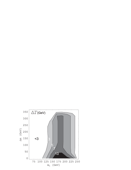
The width of a 500 GeV Higgs in the SM is $\Gamma_{SM}\approx 68$ GeV [20] (mostly due to decays into $WW$,$ZZ$ and $t$ $\bar{t}$). If $\Delta\Gamma$ reaches $0.1\,\Gamma_{SM}$, it can be seen with high luminosity at the LHC. The size of $\Delta\Gamma$ is uncertain, with strong dependence on $\lambda_{3}$ and on how many channels are open. The maximal $\Delta\Gamma$ attainable for a given $m_{\text{L }}$and $\Delta m$ is possible to estimate by letting $\lambda_{\text{L}}$ vary in the range (35) determined by the naturalness and perturbativity. The resulting $\Delta\Gamma_{\max}$ is plotted in Fig. 7. We see that there is a region where $\Delta\Gamma_{\max}\gtrsim 7$ GeV with prospects for the LHC observation.

Figure 7: Contours of the increase in the width of a 500 GeV Higgs, $\Delta\Gamma$, computed with the maximal couplings allowed by naturalness and perturbativity.

4 Alternatives

Given the indirect nature of the information contained in the EWPT, there may be and there are in fact other ways to make a heavy Higgs compatible with them. A discussion of some of the explored possibilities has been given in Ref. [3]. With reference to this discussion, we point out two related facts:

1. If the new physics responsible for allowing a heavy Higgs brings in new 4-fermion interactions, it is crucial to check that such new interactions pass the constraints set by LEP2. A relevant example in this sense is provided by the way the Kaluza Klein excitations of the SM gauge bosons affect the EWPT. While their exchange gives effects that indeed allow a good fit of the EWPT with a heavy Higgs (up to 500 GeV) [21], this fit becomes disfavoured by the newer LEP2 data [22].

2. If one tries a fit of the EWPT with a heavy Higgs, including also the LEP2 data, by adding, one at a time, the four dimension-6 operators involving the SM Higgs and gauge bosons, but not the fermions, a successful fit is obtained only from the 4-Higgs operator that corrects $T$ [22]

$$\mathcal{O}_{H}=|H^{\dagger}D_{\mu}H|^{2}.$$ (50)

This may be of some significance, since this operator is the only one that breaks custodial symmetry. So it is relatively easier to correct $T$ only, by adjusting the symmetry breaking parameter(s) that control custodial symmetry, as we do in the Inert Doublet Model.

As already said, there are other ways of correcting only, or predominantly, $T$ by some perturbative new physics. As examples, we mention here two possibilities.

i) A scalar triplet of zero hypercharge, $\tau$, [23] coupled to the SM Higgs via the potential

$$\Delta V=M^{2}\tau^{2}-m\tau_{a}H^{\dagger}\sigma_{a}H.$$ (51)

ii) A vector-like fermion doublet $F,F^{c}$ of hypercharge 1/2 and a singlet fermion $S$ with mass and interaction Lagrangian

$$\Delta\mathcal{L}=\lambda FHS+\lambda^{c}F^{c}H^{\dagger}S+MFF^{c}+\mu S^{2}.$$ (52)

Both these cases allow to correct predominantly $T$, so that a heavy Higgs becomes consistent with all current information. In our view, the drawback of the triplet model is that it corrects $T$ at tree level, so that, depending on the ratio $m/M$ all the extra particles can be hidden at inaccessible energies, up to 4-5 TeV. The fermionic example is definitely more constrained since $T$ receives one loop corrections. It also contains a DM candidate. We nevertheless find it less compelling than the IDM.

It is in fact natural at this point to ask how the IDM compares with the case where the second Higgs doublet acquires a non-zero vev. This can also be a way to improve naturalness [5]. It should be noted, however, that distributing the vevs among the 2 doublets, each smaller than $v$, strengthens the bounds on the cutoff of the loops induced by the quartic self-couplings. Furthermore, insisting on natural flavour conservation leads to unobserved massless Goldstone bosons in the limit of exact custodial symmetry. In particular, to make the charged scalar heavy enough not to conflict with direct bounds may lead to large contributions to the T parameter. A study of the consistency of the 2HDM with the EWPT in the space of its parameters has been discussed in Ref. [24].

5 Conclusions

The Large Hadron Collider will explore for the first time an energy domain well above the Fermi scale. Having in mind that $\Lambda_{QCD}$ is the only other fundamental scale known in particle physics, the importance of this fact cannot be overestimated. At the same time we are faced with the success of the SM, minimally extended to account for neutrino masses, in describing all known data in particle physics. Which physics will be revealed by the LHC?

Among the many lines of thought that have been followed to try to answer this question, on one view there is a quite general consensus: the SM is likely to be the low energy approximation of a more complete theory characterized by one or more higher physical scales. Is this telling us something about the complete theory itself? Not the least property of the SM is that its Lagrangian is the most general renormalizable one for the given gauge symmetry and particle content. Indeed this apparently allows the SM to be viewed as the infrared physics of a broad class of theories. All that one needs is to maintain gauge invariance and to produce a low energy spectrum that matches the degrees of freedom of the SM. Yet, this last property appears to be non-trivial due to the presence of the Higgs field. On one side the Higgs is crucial to the success of the SM in its perturbative description of the data. On the other side, well identified quantum corrections act to push away the Higgs from the low energy spectrum of the more complete theory. This is the naturalness problem of the SM. The problem is particularly compelling in view of the relatively large numerical size of the relevant quantum corrections, even cut off at an energy scale well inside the putative range of energies directly explorable at the LHC. Hence the effort to search for compensating effects that could be present in the complete theory, of which supersymmetry is the neatest example. In this view, the LHC will discover the new physics that cancels the leading quadratic divergences of the SM.

In this paper we have pursued a different line to attack the naturalness problem of the SM, more modest in scope but physically well motivated, we believe. The sensitivity of the Higgs mass to the cutoff is after all a quantitative issue, both for the impact on the physics expected at the LHC and in connection with the “LEP paradox” or the “little hierarchy problem”[4]. What then if a new physics effect exists which does not counteract the quadratic divergence of the Higgs mass but nevertheless relaxes the constraint on the cutoff that is inferred from it? We propose that such an effect may be due to the presence of a second Higgs doublet which, however, does not acquire a vev. We find this the simplest way to allow a heavier mass for the SM Higgs, between 400 and 600 GeV, while keeping full consistency with the EWPT. In turn a heavier Higgs makes the size of its quantum corrections less significant: the most important effect is no longer due to the top loop, as in the unmodified SM, but rather to the loop due to the Higgs self-coupling. As a consequence, strictly without any cancellation, the cutoff is pushed to about $1.5$ TeV, against a value of 400 GeV in the SM with a Higgs mass of 115 GeV. All this happens in a perfectly controllable perturbative regime for the entire extended model.

The potential of the extended Higgs sector, with a parity symmetry to keep natural flavour conservation, has 7 parameters, which can be traded for the Z mass (the vev of the SM Higgs), 4 masses of the scalar particles, 3 neutral and one charged, and 2 quartic couplings. This potential can support 2 approximate global symmetries: a custodial symmetry, which controls the splittings among the 3 inert scalars, and a Peccei-Quinn symmetry, which governs specifically the splitting among the two neutral inert bosons. While the SM Higgs mass is between 400 and 600 GeV, the other scalars have a mass ranging from 60 GeV to about 1 TeV. They are always produced in pairs and do not couple to fermions. It is an interesting question to see if, in the low mass range, their signals can be seen above background at the LHC.

The lightest of the inert scalars is necessarily stable and is required by cosmology to be neutral. If the Dark Matter is fully accounted for by this scalar, its mass is predicted to be around 70 GeV, with a small splitting of 5–10 GeV, controlled by the Peccei-Quinn symmetry, relative to the other neutral inert scalar, of opposite parity. The pair production of these neutral bosons may have barely escaped detection at LEP2, due to the small mass splitting. The cross section on protons of the DM particle is predicted to be a few times $10^{-9}$ pb, giving a signal below the present limits on direct DM searches but within the sensitivity of experiments currently under study.

We have stated in the very first paragraph of the Introduction how we view the status of the EWSB problem in this last year of the pre-LHC era. The predominant picture, rooted on supersymmetry and theoretically very appealing, is not without problems. Even more importantly, we find it difficult to say anything new on it without further experimental inputs. On the other hand we wonder if alternative roads to LHC physics cannot still be explored. We have proposed one based on a fully explicit model.

Appendix A Heavy Higgs RG flow

Detailed treatments of the Landau pole constraint in the SM exist [25]. We will find it instructive to rederive some of the known results from first principles, focussing on the heavy Higgs case. The one-loop RG equation for the SM Higgs self-coupling is

$$\frac{d\lambda}{d\ln\Lambda}=\frac{3\lambda^{2}}{2\pi^{2}}+\ldots\text{,}$$ (53)

where … stands for the gauge boson and top quark contributions, which are sub-dominant for heavy Higgs. As discussed below, the appropriate initial condition for the RG evolution is

$$\lambda(1.36m_{h})=\frac{m_{h}^{2}}{4v^{2}}\equiv\lambda_{\text{phys}},$$ (54)

where the physical Higgs mass $m_{h}$ and its vev $v$ are observable quantities. The coupling thus evolves as

$$\lambda(\Lambda)=\frac{\lambda_{\text{phys}}}{1-\frac{3\lambda_{\text{phys}}}{2\pi^{2}}\ln\frac{\Lambda}{1.36m_{h}}}\,$$ (55)

and blows up at the Landau pole

$$\Lambda_{L}=1.36m_{h}\exp\left(\frac{2\pi^{2}}{3\lambda_{\text{phys}}}\right)\,.$$ (56)

In practice, perturbation theory will break down before $\Lambda_{L}$ is reached. Let us therefore loosely define the perturbativity scale $\Lambda_{P}$ at which the one-loop correction to $\lambda$ reaches 30% of the tree-level value:

$$\Lambda_{P}=1.36m_{h}\exp\left(0.3\frac{2\pi^{2}}{3\lambda_{\text{phys}}}\right)\,.$$ (57)

The values of $\Lambda_{L,P}$ for the Higgs masses in the 400$-$600 GeV range are given in Table 1 and discussed in Section 2.2.

Let us now derive the initial condition (54) for the RG evolution (53). These initial conditions can be read off from the leading logarithmic dependence of the physical coupling $\lambda_{\text{phys }}$ on the bare parameters of the Lagrangian, provided that we take care to compute the precise denominator in the logarithm. We start from the bare Higgs Lagrangian

$$L=|\partial H|^{2}-(-\mu_{0}^{2}|H|^{2}+\lambda_{0}|H|^{4}),\quad\lambda_{0}=\lambda(\Lambda),$$ (58)

defined with a cutoff $\Lambda$. At the tree level we have

$$v^{2}=\mu_{0}^{2}/2\lambda_{0},\quad m_{h}^{2}=2\mu_{0}^{2}.$$ (59)

At the one-loop level the vev should be determined by imposing the vanishing tadpole condition $\langle h\rangle=0$. The Higgs self-energy gets non-trivial contributions only from the virtual Higgs pair and Goldstone pair diagrams. We find the following relation between the (one-loop corrected) vev and the physical Higgs mass:

$$\frac{m_{h}^{2}}{4v^{2}}=\lambda_{0}-\frac{3\lambda_{0}^{2}}{2\pi^{2}}\ln\frac{\Lambda}{C\,m_{h}}\text{,\qquad}C\approx 1.36\,.$$ (60)

Notice that the coefficient of the logarithm agrees with (53), as it should. Since the self-energy correction is evaluated at the external momentum $p^{2}=m_{h}^{2}$, it come as no suprise that $m_{h}$ appears in the denominator; the exact coefficient 1.36 is found by keeping track of finite terms. The initial condition (54) follows immediately, since the correction vanishes precisely at $\Lambda=1.36m_{h}$.

Appendix B 2HDM renormalization group equations

The one-loop renormalization group equations of the two-Higgs doublet model, referred to in Section 3.2, are:

$$16\pi^{2}\frac{d\lambda_{i}}{d\log\Lambda}=\beta_{i}(\lambda)$$

$$\beta_{1} =24\lambda_{1}^{2}+2\lambda_{3}^{2}+2\lambda_{3}\lambda_{4}+\lambda_{4}^{2}+\lambda_{5}^{2}$$

$$\beta_{2} =24\lambda_{2}^{2}+2\lambda_{3}^{2}+2\lambda_{3}\lambda_{4}+\lambda_{4}^{2}+\lambda_{5}^{2}$$

$$\beta_{3} =(12\lambda_{3}+4\lambda_{4})(\lambda_{1}+\lambda_{2})+4\lambda_{3}^{2}+2\lambda_{4}^{2}+2\lambda_{5}^{2}$$ (61)

$$\beta_{4} =4\lambda_{4}(\lambda_{1}+\lambda_{2})+4\lambda_{4}^{2}+8\lambda_{3}\lambda_{4}+8\lambda_{5}^{2}$$

$$\beta_{5} =4\lambda_{5}(\lambda_{1}+\lambda_{2})+8\lambda_{3}\lambda_{5}+12\lambda_{4}\lambda_{5}.$$

Appendix C Inert doublet contributions to $S,T$

We will derive one-loop EWPT corrections induced by the inert doublet. The $\Delta\rho$ is easiest to compute by relating it to the wave-function renormalization of the Goldstones $\phi^{+}$ and $\chi$ induced by the presence of new particles[26]:

$$\Delta\rho=\delta Z_{\phi}-\delta Z_{\chi}\text{.}$$ (62)

The relevant cubic interaction Lagrangian between the Goldstones and the inert particles is the last line of Eq. (67) below. Goldstone self-energies get corrected by the diagrams with virtual inert particle pairs. We find:

$$\Delta\rho =(\lambda_{4}+\lambda_{5})^{2}f(m_{{}_{H}},m_{S})+(\lambda_{4}-\lambda_{5})^{2}f(m_{{}_{H}},m_{A})-4\lambda_{5}^{2}f(m_{H},m_{S})$$ (63)

$$f(m_{1},m_{2}) =\frac{v^{2}}{32\pi^{2}}\int_{0}^{1}\frac{dx\,x(1-x)}{xm_{1}^{2}+(1-x)m_{2}^{2}}.$$ (64)

Using (13), it is not difficult to show that this expression is equivalent to (27).

To find $\Delta S$, we look at the gauge boson self-energy correction $\Delta\Pi_{BW^{3}}$ due to the virtual $H^{+}H^{-}$ and $SA$ loops. We find:

$$\Delta S=\frac{1}{2\pi}\int dx\,x(1-x)\ln\frac{xm_{S}^{2}+(1-x)m_{A}^{2}}{m_{H}^{2}}.$$ (65)

This $\Delta S$ is typically small: $|\Delta S|\lesssim 0.1$ in the region satisfying the naturalness and perturbativity constraints (the same region as used for determining the typical range of $\Delta T,$ Fig. 2), $-0.04\lesssim\Delta S\lesssim-0.01$ if the $\Delta T$ constraint (31) is imposed. Thus it has no significant effect on the EWPT fit.

Appendix D Dark Matter (co)annihilation cross sections

D.1 Annihilation into gauge bosons

This process is dominant above the $WW$ threshold. Since the resulting DM abundance will be very small, we will be content with a rough estimate of the cross section. In particular, we will compute the annihilation amplitudes in the massless final state approximation. This will be accurate for $m\gg m_{W}$, and will provide an order-of-magnitude estimate otherwise. The threshold behavior can be approximated by multiplying with phase space suppression factors.

We consider annihilation into transverse and longitudinal states separately. For transverse final states the amplitude is due to the contact term interactions:

$$(\sigma_{\text{LL}\rightarrow\perp\perp})v_{\text{rel}}\approx\frac{g^{4}}{64\pi m_{\text{L}}^{2}}\left(2+1/c^{4}\right)\approx 130\text{ pb }\left(100\text{ GeV}/m_{\text{L}}\right)^{2}.$$ (66)

Annihilation into longitudinal states can be approximated by annihilation into massless Goldstones. The relevant terms in the expansion of (9) are

$$V \supset\frac{1}{4}(A^{2}+S^{2})\bigl{[}2\lambda_{3}\phi^{+}\phi^{-}+(\lambda_{3}+\lambda_{4})\chi^{2}\bigr{]}+\frac{\lambda_{5}}{4}(A^{2}-S^{2})\chi^{2}$$

$$+\frac{v}{\sqrt{2}}\bigl{[}2\lambda_{1}\left(2\phi^{+}\phi^{-}+\chi^{2}\right)+\lambda_{A}A^{2}+\lambda_{S}S^{2}\bigr{]}h$$ (67)

$$+\frac{v}{\sqrt{2}}\Bigl{\{}\bigl{[}(\lambda_{4}+\lambda_{5})S+i(\lambda_{4}-\lambda_{5})A\bigr{]}H^{-}\phi^{+}+\text{c.c.}\Bigr{\}}+\sqrt{2}v\lambda_{5}SA\chi\text{.}$$

We find:

$$\mathcal{M}_{SS,AA\rightarrow\chi\chi} =\lambda_{A,S}+\frac{\lambda_{S,A}m_{h}^{2}}{s-m_{h}^{2}}+2\lambda_{5}^{2}v^{2}\left(\frac{1}{t-m_{A,S}^{2}}+\frac{1}{u-m_{A,S}^{2}}\right)$$ (68)

$$\mathcal{M}_{SS,AA\rightarrow\phi^{+}\phi^{-}} =\lambda_{3}+\frac{\lambda_{S,A}m_{h}^{2}}{s-m_{h}^{2}}+\frac{(\lambda_{4}\pm\lambda_{5})^{2}v^{2}}{2}\left(\frac{1}{t-m_{H}^{2}}+\frac{1}{u-m_{H}^{2}}\right)$$ (69)

$$\mathcal{M}_{SA\rightarrow\phi^{+}\phi^{-}} =i\frac{(\lambda_{4}^{2}-\lambda_{5}^{2})v^{2}}{2}\left(\frac{1}{t-m_{H}^{2}}-\frac{1}{u-m_{H}^{2}}\right).$$ (70)

At freezeout we can neglect $t,u$ compared to $m_{I}^{2}$; in particular, coannihilations are suppressed. The LIP annihilation amplitudes can be written as

$$\mathcal{M}_{\text{LL}\rightarrow\chi\chi} \approx\frac{\lambda_{\text{L}}s}{s-m_{h}^{2}}+2|\lambda_{5}|-\frac{4\lambda_{5}^{2}v^{2}}{m_{\text{NL}}^{2}}$$

$$\mathcal{M}_{\text{LL}\rightarrow\phi^{+}\phi^{-}} \approx\frac{\lambda_{\text{L}}s}{s-m_{h}^{2}}+|\lambda_{4}|+|\lambda_{5}|-\frac{(|\lambda_{4}|+|\lambda_{5}|)^{2}v^{2}}{m_{H}^{2}}.$$ (71)

We see that these amplitudes depend on $\lambda_{\text{L}}$, which can vary in a certain range (see Section 3.5). Because of this it can happen that one of the two amplitudes (71) is small, but not both. Indeed, the total annihilation cross section into longitudinal states can be bounded from below in a $\lambda_{\text{L}}$-independent way as follows:

$$(\sigma_{\text{LL}\rightarrow\|\|})v_{\text{rel}} \approx\frac{1}{64\pi m_{\text{L}}^{2}}(|\mathcal{M}_{\text{LL}\rightarrow\chi\chi}|^{2}+2|\mathcal{M}_{\text{LL}\rightarrow\phi^{+}\phi^{-}}|^{2})$$ (72)

$$\geq\frac{1}{64\pi m_{\text{L}}^{2}}\frac{2}{3}[\mathcal{M}_{\text{LL}\rightarrow\chi\chi}-\mathcal{M}_{\text{LL}\rightarrow\phi^{+}\phi^{-}}]^{2}$$ (73)

$$=\frac{1}{96\pi m_{\text{L}}^{2}}\left(|\lambda_{4}|-|\lambda_{5}|-\frac{(|\lambda_{4}|+|\lambda_{5}|)^{2}v^{2}}{m_{H}^{2}}+\frac{4\lambda_{5}^{2}v^{2}}{m_{\text{NL}}^{2}}\right)^{2}.$$ (74)

We have studied the last expression (which in most cases will be an underestimate) in the typical range of masses $m_{\text{L}}$, $m_{\text{NL }}$ described in Section 3.5 and found that it gives a numerical lower bound:

$$(\sigma_{\text{LL}\rightarrow\perp\perp}+\sigma_{\text{LL}\rightarrow\|\|})v_{\text{rel}}\gtrsim\min[130\text{ pb }\left(100\text{ GeV}/m_{\text{L}}\right)^{2},10\text{ pb], \quad for}\;\;\;m_{\text{L}}=(100\text{--}800)\text{ GeV.}$$ (75)

The important point is that the bound (74) is increasing with $m_{\text{L}}$, because the growth of the couplings compensates for the $m_{\text{L}}^{-2}$ suppression. As a result, the sum of (66) and (74) is above 10 pb in the whole range of $m_{\text{L}}$.

D.2 Co-annihilation into fermions

Below the $WW$ threshold, the p-wave suppressed process $SA\rightarrow Z^{*}\rightarrow\bar{f}f$ is dominant. The cross section is

$$\sigma v_{\text{rel}} =bv_{\text{rel}}^{2}$$ (76)

$$b =\left(\frac{g}{2c_{\text{w}}}\right)^{4}\frac{\sum(g_{V}^{2}+g_{A}^{2})}{96\pi m_{\text{L}}^{2}[1-m_{Z}^{2}/(4m_{\text{L}}^{2})]^{2}}\text{,}$$ (77)

where the sum is over all SM fermions, $f$, except for the top quark, and $\Delta m\ll m_{L}$. In the range of interest, we have

$$b\approx(250\text{--}60)\text{ pb},\qquad m_{\text{L}}=(60\text{--}80)\text{ GeV.}$$ (78)

For $\Delta m<T$, the thermally averaged cross section which enters the Boltzmann equation is $\langle\sigma v_{\text{rel}}\rangle=6b/x,$ $x=m/T$.

References

- [1] The LEP Collaborations ALEPH, DELPHI, L3, OPAL, and the LEP Electroweak Working Group, “A combination of preliminary electroweak measurements and constraints on the standard model,” arXiv:hep-ex/0511027.
- [2] M. B. Einhorn, D. R. T. Jones and M. J. G. Veltman, “Heavy Particles And The Rho Parameter In The Standard Model,” Nucl. Phys. B 191 (1981) 146.
- [3] M. E. Peskin and J. D. Wells, “How can a heavy Higgs boson be consistent with the precision electroweak measurements?,” Phys. Rev. D 64, 093003 (2001) [arXiv:hep-ph/0101342].
- [4] R. Barbieri and A. Strumia, “The ’LEP paradox’,” arXiv:hep-ph/0007265.
- [5] R. Barbieri and L.J. Hall “Improved Naturalness and the Two Higgs Doublet Model,” arXiv:hep-ph/0510243.
- [6] T. Gregoire, D. R. Smith and J. G. Wacker, “What precision electroweak physics says about the SU(6)/Sp(6) little Higgs,” Phys. Rev. D 69 (2004) 115008 [arXiv:hep-ph/0305275].
- [7] M. J. G. Veltman, “The Infrared - Ultraviolet Connection,” Acta Phys. Polon. B 12, 437 (1981).
- [8] http://lepewwg.web.cern.ch/LEPEWWG/plots/summer2005/s05_stu_contours.eps
- [9] S. L. Glashow and S. Weinberg, “Natural Conservation Laws For Neutral Currents,” Phys. Rev. D 15, 1958 (1977).
- [10] E. Ma, “Verifiable radiative seesaw mechanism of neutrino mass and dark matter,” arXiv:hep-ph/0601225.
- [11] Particle Data Group, http://pdg.lbl.gov, Searches for WIMPs and Other Particles.
- [12] The CDMS Collaboration, “Limits on spin-independent WIMP nucleon interactions from the two-tower run of the Cryogenic Dark Matter Search,” Phys. Rev. Lett. 96, 011302 (2006) [arXiv:astro-ph/0509259].
- [13] E. W. Kolb and M. S. Turner, “The Early Universe,” Addison-Wesley (1990).
- [14] K. Griest and D. Seckel, “Three Exceptions In The Calculation Of Relic Abundances,” Phys. Rev. D 43, 3191 (1991).
- [15] R. Barbieri, M. Frigeni and G. F. Giudice, “Dark Matter Neutralinos In Supergravity Theories,” Nucl. Phys. B 313 (1989) 725.
- [16] M. Cirelli, N. Fornengo and A. Strumia, “Minimal dark matter,” arXiv:hep-ph/0512090.
-
[17]
The DELPHI Collaboration, “Searches for supersymmetric
particles in collisions up to 208 GeV and interpretation of the
results within the MSSM,” Eur. Phys. J. C 31, 421 (2004)
[arXiv:hep-ex/0311019];
The OPAL Collaboration, “Search for chargino and neutralino production at -209 GeV to at LEP,” Eur. Phys. J. C 35, 1 (2004) [arXiv:hep-ex/0401026];
The L3 Collaboration, “Search for charginos and neutralinos in e+ e- collisions at GeV,” Phys. Lett. B 472, 420 (2000) [arXiv:hep-ex/9910007]. - [18] T. Sjostrand, P. Eden, C. Friberg, L. Lonnblad, G. Miu, S. Mrenna and E. Norrbin, “High-energy-physics event generation with PYTHIA 6.1,” Comput. Phys. Commun. 135, 238 (2001) [arXiv:hep-ph/0010017].
- [19] R. Barbieri, F. Caravaglios, M. Frigeni and M. L. Mangano, “Production and leptonic decays of charginos and neutralinos in hadronic collisions,” Nucl. Phys. B 367 (1991) 28.
- [20] A. Djouadi, “The anatomy of electro-weak symmetry breaking. I: The Higgs boson in the standard model,” arXiv:hep-ph/0503172.
- [21] A. Strumia, “Bounds on Kaluza-Klein excitations of the SM vector bosons from electroweak tests,” Phys. Lett. B 466, 107 (1999) [arXiv:hep-ph/9906266].
- [22] R. Barbieri, A. Pomarol, R. Rattazzi and A. Strumia, “Electroweak symmetry breaking after LEP1 and LEP2,” Nucl. Phys. B 703, 127 (2004) [arXiv:hep-ph/0405040].
- [23] J. R. Forshaw, D. A. Ross and B. E. White, “Higgs mass bounds in a triplet model,” JHEP 0110 (2001) 007 [arXiv:hep-ph/0107232].
- [24] P. H. Chankowski, T. Farris, B. Grzadkowski, J. F. Gunion, J. Kalinowski and M. Krawczyk, “Do precision electroweak constraints guarantee e+ e- collider discovery of at least one Higgs boson of a two Higgs doublet model?,” Phys. Lett. B 496 (2000) 195 [arXiv:hep-ph/0009271].
- [25] T. Hambye and K. Riesselmann, “Matching conditions and Higgs mass upper bounds revisited,” Phys. Rev. D 55, 7255 (1997) [arXiv:hep-ph/9610272].
- [26] R. Barbieri, M. Beccaria, P. Ciafaloni, G. Curci and A. Vicere, “Two loop heavy top effects in the Standard Model,” Nucl. Phys. B 409 (1993) 105.