Instability of a gapless color superconductor with respect to inhomogeneous fluctuations

Abstract

We systematically apply density functional theory to determine the kind of inhomogeneities that spontaneously develop in a homogeneous gapless phase of neutral two-flavor superfluid quark matter. We consider inhomogeneities in the quark and electron densities and in the phases and amplitude of the order parameter. These inhomogeneities are expected to lead the gapless phase to a BCS-normal coexisting phase, a Larkin-Ovchinnikov-Fulde-Ferrell (LOFF) state with phase oscillations alone, and a LOFF state with amplitude oscillations. We find that which of them the homogeneous system tends towards depends sensitively on the chemical potential separation between up and down quarks and the gradient energies.

I Introduction

It has been noted since the seminal work in Refs. barrois ; BL that the quark-quark interaction in the color antitriplet channel is attractive and drives a Cooper pairing instability in quark matter in the limit of high density. In this limit, the ground state for three-flavor quark matter is a homogeneous color-flavor locked state in which all nine quarks, associated with three colors and three flavors, are gapped ARW . However, color superconducting states, if occurring in compact stars, would not be necessarily homogeneous. This is because a separation of the Fermi surface develops between paired quarks in a realistic situation characterized by nonzero strange quark mass, color and electric charge neutrality, and weak equilibrium. Once the separation becomes comparable to the gap magnitude, a usual BCS state can be energetically unfavorable because of the inevitable increase in the loss of the quark kinetic energy. Even in this situation, it is possible to consider other homogeneous paired states such as a gapless state in which quark quasiparticles which are gapped in the absence of the Fermi surface separation become gapless GLW ; SH ; AKR , a color-flavor locked state with condensation of collective modes carrying the same quantum number as mesons BSKR , and a paired state with nonspherical Fermi surfaces MS . Importantly, these homogeneous states are not always stable against inhomogeneities. The most remarkable example is a chromomagnetic instability of the gapless states which is characterized by negative Meissner masses squared HS2 ; CN ; this signifies that fluctuations in the gluon fields or, equivalently, the phases of the order parameter GR , develops spontaneously. [Note that in an overall neutral system of charged fermions, the gapless states can be stable against homogeneous change in the gap magnitude in contrast to the case of neutral Fermi systems (see Ref. Forbes for an exception).] So far, many states involving inhomogeneities in the quark densities and/or the order parameter Shov have been proposed for an eventual stable state after the onset of the chromomagnetic instability, but a systematic energy comparison between them and even a systematic instability analysis with respect to various possible inhomogeneities remain to be performed.

In this paper, as a first step towards such a systematic analysis, we utilize density functional theory to investigate instabilities of a two-flavor homogeneous gapless state with respect to inhomogeneous fluctuations in the quark and electron densities and in the phases and amplitude of the order parameter. Here we do not address what the ground state is, but all we can clarify is to identify inhomogeneities that grow spontaneously in the homogeneous system, from which we can anticipate what kind of inhomogeneous state is likely to be realized. Possibly, the growth of fluctuations in the phases and/or amplitude of the order parameter would end up with a Larkin-Ovchinnikov-Fulde-Ferrell (LOFF) state LOFF in which periodic spatial oscillations occur in the phases and/or amplitude, while the simultaneous growth of fluctuations in the density difference between up and down quarks and the gap magnitude could lead to a BCS-normal coexisting phase BCR ; RR . We take into account finite size corrections such as the energies arising from the density and gap gradients and the electrostatic and color Coulomb energies to deduce the structure of the coexisting phase. We find that electric charge screening, which is automatically included in the present density functional analysis, is crucial to such deduction. The coexisting phase and the LOFF phase with amplitude modulations are related with each other in the sense that both phases involve nonzero amplitude and density modulations. As we will see later, it is the competition between the density and gap gradient energies that determines which of these the system prefers to go to when the system is unstable with respect to fluctuations in the gap magnitude.

In Sec. II, we summarize the bulk properties of homogeneous color superconducting states in two-flavor neutral quark matter at zero temperature. Section III is devoted to constructing density functional theory, by including not only the bulk properties summarized in Sec. II but also inhomogeneities in the order parameter and the densities of the constituents, and to classifying possible instabilities of the gapless state. In Sec. IV, we calculate the effective potential for the gap magnitude and thereby clarify how the type of instabilities changes with the Fermi surface separation and a parameter characterizing the density gradient energy. Our conclusions are given in Sec. V. We use units in which $\hbar=c=k_{B}=1$.

II Homogeneous phases

In this section we summarize the bulk properties of two-flavor neutral $\beta$ equilibrated quark matter at zero temperature by using a simple BCS type model. This is instructive for a later stability analysis, which requires the second derivatives of the thermodynamic potential density with respect to the phases and magnitude of the order parameter and the quark and electron densities.

We consider uniform $ud$-flavor quark matter of baryon chemical potential $3\mu$ and zero temperature. We assume that the system is in weak equilibrium with the gas of electrons of chemical potential $\mu_{e}$ and has zero net color and electric charge. We neglect quark and electron masses, and chiral and meson condensates. For a normal state, we simply adopt the ideal gas form of the thermodynamic potential density,

$$\Omega_{\rm normal}=-\frac{1}{12\pi^{2}}\sum_{i=e,q}\mu_{i}^{4},$$ (1)

where $q\equiv fa$ stands for the set of color $a=R,G,B$ and flavor $f=u,d$, and $\mu_{q}$ is the chemical potential of $q$ quarks. In this case, $\beta$ equilibrium and charge neutrality lead to

$$\mu_{q}=\mu-Q_{q}\mu_{e},$$ (2)

where $Q_{q}$ is the electric charge of $q$ quarks. The number density of $i$ particles are then given by the corresponding chemical potentials $\mu_{i}$ as

$$n_{i}=\frac{\mu_{i}^{3}}{3\pi^{2}}.$$ (3)

Let us then consider a two-flavor color superconducting (2SC) state in which Cooper pairing occurs in a $J^{P}=0^{+}$, isoscalar, and $RG$-color antitriplet channel. For a pairing interaction, we adopt a contact interaction,

$$-G_{D}(\bar{\psi}_{fa}P_{ab}^{fh}\psi^{C}_{hb})(\bar{\psi}^{C}_{f^{\prime}a^{\prime}}P_{a^{\prime}b^{\prime}}^{f^{\prime}h^{\prime}}\psi_{h^{\prime}b^{\prime}}),$$ (4)

where $P_{ab}^{fh}=i\gamma_{5}\epsilon_{fh}\epsilon_{abB}$, $\psi_{fa}$ is the quark spinor of color $a$ and flavor $f$, and $\psi_{fa}^{C}=i\gamma^{2}\gamma^{0}{\bar{\psi}}_{fa}^{T}$. Here we assume that this pairing interaction is cut off unless the transfer of the relative momentum of paired quarks is smaller than $\Lambda$ in magnitude. In some sense this cutoff can be considered to simulate the instanton form factor RSSV , which allows us to solve the gap equation in the same way as the original BCS case in which the cutoff is given by the Debye frequency. We take $\Lambda$ as 300 MeV, which is small compared with a typical value of the Fermi energy of order 500 MeV. Hereafter we will often assume $\Delta\ll\Lambda$; this is reasonable for a typical range of $\Delta$ of 0–100 MeV.

Within the mean-field approximation, the pairing gap $\Delta$ is related to the diquark condensate as

$$\Delta=2G_{D}\langle\bar{\psi}_{fa}P_{ab}^{fh}\psi^{C}_{hb}\rangle,$$ (5)

with the ensemble average $\langle\cdots\rangle$. Taking note of this relation, it is straightforward to write down the thermodynamic potential density as SH

$$\Omega_{\rm 2SC}\! = \!-\frac{1}{12\pi^{2}}\!\sum_{i=e,uB,dB}\!\mu_{i}^{4}-\frac{1}{12\pi^{2}}\!\!\sum_{i=uR,dR,uG,dG}\!\!{\bar{\mu}}^{4}+\frac{\Delta^{2}}{4G_{D}}-\frac{1}{2\pi^{2}}\!\!\sum_{i=uR,dR,uG,dG}\!\!\int_{{\bar{\mu}}-\Lambda}^{{\bar{\mu}}+\Lambda}dpp^{2}\left[\sqrt{(p-{\bar{\mu}})^{2}+\Delta^{2}}-|p-{\bar{\mu}}|\right]$$ (6)

$$\simeq -\frac{1}{12\pi^{2}}\sum_{i=e,uB,dB}\mu_{i}^{4}-\frac{1}{12\pi^{2}}\sum_{i=uR,dR,uG,dG}{\bar{\mu}}^{4}+\frac{\Delta^{2}}{4G_{D}}-\frac{{\bar{\mu}}^{2}\Delta^{2}}{2\pi^{2}}\sum_{i=uR,dR,uG,dG}\left(\frac{1}{2}+\ln\frac{2\Lambda}{\Delta}\right),$$

where

$${\bar{\mu}}\equiv\frac{\mu_{uR}+\mu_{dG}}{2}=\frac{\mu_{dR}+\mu_{uG}}{2},$$ (7)

and $p$ is the quasiparticle momentum associated with paired quarks. We have assumed $\Delta\ll\Lambda$ in the approximate estimate. Weak equilibrium and color and electric charge neutrality ensure

$$\mu_{fa}=\mu-Q_{f}\mu_{e}+Q^{\alpha=8}_{a}\mu_{8},$$ (8)

where $Q^{\alpha=8}_{a}\equiv(1/3,1/3,-2/3)$ is the color charge for gluon color index $\alpha=8$, and $\mu_{8}$ is the associated color chemical potential. The chemical potentials $\mu_{e}$ and $\mu_{8}$ are determined by the neutrality conditions,

$$\frac{\partial\Omega_{\rm 2SC}}{\partial\mu_{e}}=\frac{\partial\Omega_{\rm 2SC}}{\partial\mu_{8}}=0.$$ (9)

From these conditions, one can show that in the 2SC state, $\mu_{e}$ is related to $\mu$ and $\mu_{8}$ as $\mu_{e}=(3\mu-2\mu_{8})/5$, while $\mu_{8}\approx 0.0854\mu$ up to leading order in $\Delta/\mu$ SH .

We then calculate the gap and the number densities from $\Omega_{\rm 2SC}[\Delta;\mu_{i}]$ given by Eq. (6). Variation of $\Omega_{\rm 2SC}$ with respect to the gap gives rise to the gap equation,

$$0=\frac{\partial\Omega_{\rm 2SC}}{\partial\Delta}=\frac{\Delta}{2G_{D}}-\frac{4{\bar{\mu}}^{2}\Delta}{\pi^{2}}\ln\frac{2\Lambda}{\Delta}.$$ (10)

This is identical with the form of the usual BCS gap equation. We define the gap satisfying Eq. (10) as $\Delta=\Delta_{\rm 2SC}$. The number densities for $i=e,uB,dB$ are still given by Eq. (3), while for $i=uR,uG,dR,dG$ we obtain, up to leading order in $\Delta/\Lambda$,

$$n_{i}\simeq\frac{{\bar{\mu}}^{3}}{3\pi^{2}}+\frac{{\bar{\mu}}\Delta^{2}}{\pi^{2}}\ln\frac{2\Lambda}{\Delta}.$$ (11)

Obviously, the neutrality constraints (9) can be rewritten in terms of $n_{i}$ as

$$n_{e}=\sum_{fa}Q_{f}n_{fa},\qquad 0=\sum_{fa}Q^{\alpha=8}_{a}n_{fa}.$$ (12)

The 2SC state is relevant only when the separation of the Fermi surface between the $u$ and $d$ quarks,

$$\delta\mu\equiv\frac{\mu_{dG}-\mu_{uR}}{2}=\frac{\mu_{dR}-\mu_{uG}}{2}=\frac{\mu_{e}}{2},$$ (13)

is smaller than the gap $\Delta_{\rm 2SC}$ SH . This is because the smallest quasiparticle gap associated with paired quarks vanishes once the separation reaches $\Delta_{\rm 2SC}$. In fact, according to the usual Bogoliubov method, the corresponding quasiparticle energy $E_{-}(p)$ reads

$$E_{-}(p)=\sqrt{(p-{\bar{\mu}})^{2}+\Delta^{2}}-\delta\mu,$$ (14)

and for $\delta\mu=\Delta=\Delta_{\rm 2SC}$, $E_{-}({\bar{\mu}})=0$. Note that in the 2SC state the gap magnitude and thus the condensation energy is independent of $\delta\mu$ except for the slight dependence on $\delta\mu$ through ${\bar{\mu}}$ in Eq. (10). This is because quarks forming Cooper pairs are located in the middle of the Fermi surfaces as in Eq. (7), rather than around the respective Fermi surfaces.

For $\delta\mu<\Delta_{\rm 2SC}$, one can find another branch of the homogeneous solution to the gap equation in which the gap magnitude is not only smaller than $\Delta_{\rm 2SC}$ but also the separation $\delta\mu$. This state, hereafter referred to as the gapless 2SC state, is characterized by the presence of gapless quasiparticle modes associated with paired quarks. This is similar to a state originally predicted by Sarma Sarma for superconductors in external magnetic fields. The corresponding thermodynamic potential can be described, simply by adding to Eq. (6) an energy contribution from gapless quasiparticle modes of energy $E_{-}(p)$, as

$$\Omega_{\rm g2SC} = -\frac{1}{12\pi^{2}}\!\sum_{i=e,uB,dB}\!\mu_{i}^{4}-\frac{1}{12\pi^{2}}\!\!\sum_{i=uR,dR,uG,dG}\!\!{\bar{\mu}}^{4}+\frac{\Delta^{2}}{4G_{D}}-\frac{1}{2\pi^{2}}\!\!\sum_{i=uR,dR,uG,dG}\!\!\int_{{\bar{\mu}}-\Lambda}^{{\bar{\mu}}+\Lambda}dpp^{2}\left[\sqrt{(p-{\bar{\mu}})^{2}+\Delta^{2}}-|p-{\bar{\mu}}|\right]$$ (15)

$$+\frac{1}{2\pi^{2}}\sum_{i=uR,dR,uG,dG}\int_{\mu^{-}}^{\mu^{+}}dpp^{2}E_{-}(p),$$

where $\mu^{\pm}\equiv{\bar{\mu}}\pm\sqrt{(\delta\mu)^{2}-\Delta^{2}}$. Then, the gap equation reads

$$0=\frac{\partial\Omega_{\rm g2SC}}{\partial\Delta} = \frac{\Delta}{2G_{D}}-\frac{4{\bar{\mu}}^{2}\Delta}{\pi^{2}}\ln\frac{2\Lambda}{\Delta}$$ (16)

$$+2\frac{\Delta}{\pi^{2}}\left[(2{\bar{\mu}}^{2}-\Delta^{2})\ln\frac{\sqrt{(\delta\mu)^{2}-\Delta^{2}}+\delta\mu}{\Delta}+\delta\mu\sqrt{(\delta\mu)^{2}-\Delta^{2}}\right].$$

By retaining a term of leading order in $\Delta/{\bar{\mu}}$ in the contribution from the gapless modes, we obtain an approximate solution as

$$\Delta\simeq\sqrt{\Delta_{\rm 2SC}(2\delta\mu-\Delta_{\rm 2SC})},$$ (17)

which has the same form as that derived by Sarma Sarma . Note that the gap magnitude is explicitly dependent on $\delta\mu$ in contrast to the case of the 2SC state.

The number densities of quarks and electrons can be determined by the derivatives of $\Omega_{\rm g2SC}$ with respect to the chemical potentials. The number densities for $i=e,uB,dB$ are again given by Eq. (3), while for $i=uR,uG,dR,dG$ we obtain, up to leading order in $\Delta/\Lambda$,

$$n_{i} \simeq \frac{{\bar{\mu}}^{3}}{3\pi^{2}}+\frac{{\bar{\mu}}\Delta^{2}}{\pi^{2}}\ln\frac{2\Lambda}{\Delta}$$ (18)

$$\pm \frac{1}{3\pi^{2}}\sqrt{(\delta\mu)^{2}-\Delta^{2}}[3{\bar{\mu}}^{2}+(\delta\mu)^{2}-\Delta^{2}]-\frac{{\bar{\mu}}}{\pi^{2}}\left[\Delta^{2}\ln\frac{\sqrt{(\delta\mu)^{2}-\Delta^{2}}+\delta\mu}{\Delta}-\delta\mu\sqrt{(\delta\mu)^{2}-\Delta^{2}}\right],$$

where the upper and lower sign in the right side are taken for $d$ quarks and $u$ quarks, respectively.

It is instructive to note that the gapless state is stable against small homogeneous change in the gap magnitude in charged Fermi systems because of the neutrality constraints SH , although it is generally unstable in neutral Fermi systems. (In fact, without charge, at given $\delta\mu$ below $\Delta_{\rm 2SC}$, the gap magnitude and thus the condensation energy would be larger for the 2SC state than for the gapless state.) By substituting the above-obtained densities into Eq. (12), one obtains an approximate relation between $\Delta$ and $\delta\mu$ as

$$\Delta^{2}\approx(\delta\mu)^{2}-\left[\frac{(\mu-4\delta\mu/3)^{3}-(2\delta\mu)^{3}}{6(\mu-\delta\mu/3)^{2}}\right]^{2}.$$ (19)

Here we have assumed $\mu_{8}=0$, which is known to be a reasonable approximation since nonzero $\mu_{8}$ can arise solely from nonzero $\Delta$. By taking note of the condition that Eqs. (17) and (19) are compatible, we can find that the gapless state is energetically favored over the normal and 2SC states at intermediate coupling SH . In fact, the condition for the presence of the gapless and neutral solution approximately reads

$$0.11\mu\lesssim\delta\mu\lesssim\frac{3}{10}\mu.$$ (20)

(See Fig. 1 for an example of the gapless and neutral solution.) By combining this relation with the condition, $\Delta_{\rm 2SC}/2\lesssim\delta\mu\lesssim\Delta_{\rm 2SC}$, for the presence of the gapless 2SC solution, we obtain

$$0.22\mu\lesssim\Delta_{\rm 2SC}\lesssim\frac{3}{10}\mu.$$ (21)

This relation implies that above (or below) this region of $\Delta_{\rm 2SC}$, the neutral solution, that is, the intersection of the neutral constraint as shown by the dotted line in Fig. 1 and the solution of the gap equation as shown by the solid line (or the line of $\Delta=0$) in Fig. 1, lies only in the region of the 2SC (or normal) phase SH .

Figure 1: The homogeneous gap $\Delta$ as a function of $\delta\mu$ obtained for $\mu=500$ MeV and $\Delta_{\rm 2SC}(\delta\mu=0)=120$ MeV. The upper solid line is the 2SC solution, and the lower solid line is the gapless 2SC (g2SC) solution [see Eq. (17)], while the dotted line denotes the neutrality constraint [see Eq. (19)]. The intersection of the g2SC solution and the dotted line corresponds to the homogeneous neutral solution to the gap equation. Note that the real 2SC solution is dependent on $\delta\mu$ through the $\delta\mu$ dependence of $\bar{\mu}$, although such a dependence is negligible under the approximation utilized here SH .

III Instability with respect to inhomogeneities

As mentioned in the previous section, the gapless 2SC state is stable against small homogeneous change in the gap magnitude. However, it is necessary to examine the stability against inhomogeneities. In fact, it is known that the gapless 2SC state is unstable with respect to spontaneous generation of gauge fields HS2 . In this section, we construct density functional theory to analyze the stability against inhomogeneities, and then describe typical instabilities which might occur in the gapless 2SC state and even in the 2SC state.

III.1 Density functional theory

We proceed to write the energy density functional allowing for infinitesimal inhomogeneities in the phases and magnitude of the order parameter and in the quark and electron densities, i.e., the position dependent densities $n_{i}({\bf r})\equiv n_{i}+\delta n_{i}({\bf r})$, gap magnitude $\Delta({\bf r})\equiv\Delta+\delta\Delta({\bf r})$, electromagnetic field ${\bf A}({\bf r})$, and gluon fields ${\bf A}^{\alpha}({\bf r})$ (as we shall see below, any nonzero gauge fields including constant ones correspond to inhomogeneities in the phases of the order parameter). For inhomogeneities of spatial scale larger than the coherence length, it is sufficient to adopt the local density approximation for the bulk energy and keep the energies arising from the gap and density gradients up to leading order. Thus, the total thermodynamic potential for given $\mu$ reads

$$\Omega_{\rm tot}=\int d^{3}r\;\Omega_{\rm(g)2SC}(n_{i}({\bf r}),\Delta({\bf r}))+\int d^{3}r\;\Omega_{g}(n_{i}({\bf r}),\Delta({\bf r}),{\bf A}({\bf r}),{\bf A}^{\alpha}({\bf r}))+E_{C}+\sum_{\alpha}E_{C}^{\alpha}.$$ (22)

Here $\Omega_{\rm 2SC}$ and $\Omega_{\rm g2SC}$ are given by Eqs. (6) and (15),

$$\Omega_{g} = \frac{1}{2}\sum_{fhab}B_{fa,hb}(\nabla n_{fa})\cdot(\nabla n_{hb})$$ (23)

$$+2K_{T}^{(0)}\sum_{ab\alpha}\left|\left(\delta_{ab}\nabla-ig\frac{\lambda^{\alpha}_{ab}}{2}{\bf A}^{\alpha}+i\delta_{ab}\frac{e}{3}{\bf A}\right)\delta_{bB}\Delta\right|^{2}$$

$$+2K_{T}^{(1)}\sum_{ab\alpha}\left|\delta_{aB}\Delta\left(\delta_{ab}\nabla-ig\frac{\lambda^{\alpha}_{ab}}{2}{\bf A}^{\alpha}+i\delta_{ab}\frac{e}{3}{\bf A}\right)\delta_{bB}\Delta\right|^{2}$$

is the gradient energy,

$$E_{C}=\frac{1}{8\pi}\int d^{3}r_{1}\int d^{3}r_{2}\frac{\rho({\bf r}_{1})\rho({\bf r}_{2})}{|{\bf r}_{1}-{\bf r}_{2}|}$$ (24)

with

$$\rho=e\left(\sum_{fa}Q_{f}n_{fa}-n_{e}\right)$$ (25)

is the electrostatic Coulomb energy, and

$$\sum_{\alpha}E_{C}^{\alpha}=\frac{1}{8\pi}\sum_{\alpha}\int d^{3}r_{1}\int d^{3}r_{2}\frac{\rho^{\alpha}({\bf r}_{1})\rho^{\alpha}({\bf r}_{2})}{|{\bf r}_{1}-{\bf r}_{2}|}$$ (26)

with

$$\rho^{\alpha}=\frac{1}{2}g\sum_{fab}\langle\bar{\psi}_{fa}\gamma^{0}\lambda^{\alpha}_{ab}\psi_{fb}\rangle$$ (27)

is the color Coulomb energy. Here we have ignored the gluon contribution to the color density since it is of higher order in ${\bf A}^{\alpha}({\bf r})$. For the covariant derivative, we have taken the form relevant for the gap which has a $B$ direction in anti-color space, and $e/3$ corresponds to the electric charge carried by a Cooper pair. The local thermodynamic potential, up to second order in various inhomogeneities, can then be written as

$$\Omega_{\rm tot} = \Omega_{0}$$ (28)

$$+\frac{1}{2}\int d^{3}r\left[\sum_{i,j}\frac{\partial^{2}\Omega_{\rm(g)2SC}}{\partial n_{i}\partial n_{j}}\delta n_{i}({\bf r})\delta n_{j}({\bf r})+2\sum_{i}\frac{\partial^{2}\Omega_{\rm(g)2SC}}{\partial n_{i}\partial\Delta}\delta n_{i}({\bf r})\delta\Delta({\bf r})+\frac{\partial^{2}\Omega_{\rm(g)2SC}}{\partial\Delta^{2}}(\delta\Delta({\bf r}))^{2}\right]$$

$$+\frac{1}{2}\sum_{abfh}\int\frac{d^{3}q}{(2\pi)^{3}}q^{2}B_{fa,hb}\delta n_{fa}({\bf q})\delta n_{hb}^{*}({\bf q})+2(K_{T}^{(0)}+\Delta^{2}K_{T}^{(1)})\int\frac{d^{3}q}{(2\pi)^{3}}q^{2}|\delta\Delta({\bf q})|^{2}$$

$$+\frac{1}{2}\sum_{\alpha\beta}\int d^{3}r(m_{M}^{\alpha\beta})^{2}{\bf A}^{\alpha}({\bf r}){\bf A}^{\beta}({\bf r})+\frac{1}{2}\sum_{\alpha}\int d^{3}r(m_{M}^{\alpha})^{2}{\bf A}^{\alpha}({\bf r}){\bf A}({\bf r})+\frac{1}{2}\int d^{3}r(m_{M})^{2}({\bf A}({\bf r}))^{2}$$

$$+\frac{1}{2}\int\frac{d^{3}q}{(2\pi)^{3}}\frac{1}{q^{2}}|\rho({\bf q})|^{2}+\frac{1}{2}\sum_{\alpha}\int\frac{d^{3}q}{(2\pi)^{3}}\frac{1}{q^{2}}|\rho^{\alpha}({\bf q})|^{2},$$

where $\Omega_{0}$ is the thermodynamic potential of the homogeneous state, $\delta n_{i}({\bf q})$, $\delta\Delta({\bf q})$, $\rho({\bf q})$, and $\rho^{\alpha}({\bf q})$ are the Fourier transforms of the corresponding inhomogeneities, and

$$(m_{M}^{\alpha\beta})^{2}=\delta_{\alpha\beta}\left\{\begin{array}[]{ll}0,&\mbox{$\alpha=1$--3}\\ K_{T}^{(0)}g^{2}\Delta^{2},&\mbox{$\alpha=4$--7}\\ \frac{4}{3}(K_{T}^{(0)}+\Delta^{2}K_{T}^{(1)})g^{2}\Delta^{2},&\mbox{$\alpha=8$},\end{array}\right.$$ (29)

$$(m_{M}^{\alpha})^{2}=\delta_{\alpha 8}\frac{4}{3\sqrt{3}}(K_{T}^{(0)}+\Delta^{2}K_{T}^{(1)})ge\Delta^{2},$$ (30)

and

$$(m_{M})^{2}=\frac{4}{9}(K_{T}^{(0)}+\Delta^{2}K_{T}^{(1)})e^{2}\Delta^{2}$$ (31)

are the Meissner masses squared for gluon-gluon, gluon-photon, and photon-photon channels, respectively. Here we note that the first order terms vanish due to equilibrium, i.e.,

$$\frac{\partial\Omega_{\rm(g)2SC}}{\partial n_{i}}=\frac{\partial\Omega_{\rm(g)2SC}}{\partial\Delta}=0,$$ (32)

and that the terms including both ${\bf A}$ or ${\bf A}^{\alpha}$ and $\delta\Delta$ or $\delta n_{i}$ do not appear up to second order. We also neglect the electron contribution to the gradient energy, which is expected to be small compared with the quark contribution that will be discussed below.

We can simplify the color Coulomb energy by only retaining the components of $\alpha=3,8$. In fact, for $\alpha\neq 3,8$, $\rho^{\alpha}$ turns out to be zero; any deviation of $\rho^{\alpha}$ from zero for $\alpha\neq 3,8$ would result in energy increase because there is no dependence on $\rho^{\alpha}$ in the other energy terms. (Vanishing $\rho^{\alpha}$ conforms to the color neutrality $\int d^{3}r\rho^{\alpha}({\bf r})=0$.) Consequently, the color Coulomb energy can be written as the sum of $E_{C}^{\alpha=3}$ and $E_{C}^{\alpha=8}$ given by

$$E_{C}^{\alpha=3,8}=\frac{1}{2}\int\frac{d^{3}q}{(2\pi)^{3}}\left(\frac{\sqrt{3}g}{2}\right)^{2}\frac{1}{q^{2}}\left|\sum_{a}Q^{\alpha=3,8}_{a}\delta n_{a}({\bf q})\right|^{2},$$ (33)

where $\delta n_{a}=\sum_{f}\delta n_{fa}$ and $Q^{\alpha=3}_{a}=(1/\sqrt{3},-1/\sqrt{3},0)$.

For later use, we write the expressions for the second derivatives of the thermodynamic potential density as

$$\frac{\partial^{2}\Omega_{\rm(g)2SC}}{\partial\Delta^{2}}=\frac{4{\bar{\mu}}^{2}}{\pi^{2}}\left[1-\theta(\delta\mu-\Delta)\left(\frac{\delta\mu}{\sqrt{(\delta\mu)^{2}-\Delta^{2}}}+\frac{\Delta^{2}}{{\bar{\mu}}^{2}}\ln\frac{\sqrt{(\delta\mu)^{2}-\Delta^{2}}+\delta\mu}{\Delta}\right)\right],$$ (34)

$$\frac{\partial^{2}\Omega_{\rm(g)2SC}}{\partial n_{i}\partial\Delta}=\frac{\partial\mu_{i}}{\partial\Delta}=\cases{\Delta\left[-\displaystyle{\frac{2}{\bar{\mu}}}\ln\displaystyle{\frac{2\Lambda}{\Delta}}+\theta(\delta\mu-\Delta)\left(\displaystyle{\frac{2}{\bar{\mu}}}\ln\displaystyle{\frac{\sqrt{(\delta\mu)^{2}-\Delta^{2}}+\delta\mu}{\Delta}}-\displaystyle{\frac{1}{\delta\mu}}\right)\right],&\mbox{$i=uR,uG$}\cr\Delta\left[-\displaystyle{\frac{2}{\bar{\mu}}}\ln\displaystyle{\frac{2\Lambda}{\Delta}}+\theta(\delta\mu-\Delta)\left(\displaystyle{\frac{2}{\bar{\mu}}}\ln\displaystyle{\frac{\sqrt{(\delta\mu)^{2}-\Delta^{2}}+\delta\mu}{\Delta}}+\displaystyle{\frac{1}{\delta\mu}}\right)\right],&\mbox{$i=dR,dG$}\cr 0,&\mbox{$i=uB,dB,e$},\cr}$$ (35)

$$\frac{\partial^{2}\Omega_{\rm(g)2SC}}{\partial n_{i}\partial n_{j}}=\frac{\partial\mu_{i}}{\partial n_{j}}=\cases{\displaystyle{\frac{\pi^{2}}{2{\bar{\mu}}^{2}}}\left[1+\left(\theta(\delta\mu-\Delta)\displaystyle{\frac{\delta\mu}{\sqrt{(\delta\mu)^{2}-\Delta^{2}}}}\right)^{-1}\right],&\mbox{for $(i,j)=(ua,ub),(da,db)$}\cr\displaystyle{\frac{\pi^{2}}{2{\bar{\mu}}^{2}}}\left[1-\left(\theta(\delta\mu-\Delta)\displaystyle{\frac{\delta\mu}{\sqrt{(\delta\mu)^{2}-\Delta^{2}}}}\right)^{-1}\right],&\mbox{for $(i,j)=(ua,db),(da,ub)$}\cr\delta_{ij}\left(\displaystyle{\frac{\pi}{3n_{i}}}\right)^{2/3},&\mbox{for $i=uB,dB,e$}\cr 0,&\mbox{for others},\cr}$$ (36)

where $a=R,G$ and $b=R,G$. In Eqs. (35) and (36) we have ignored higher order terms with respect to $\Delta/\Lambda$ and $\Delta/{\bar{\mu}}$. In evaluating $\partial\mu_{i}/\partial\Delta$ we made use of $\partial n_{i}/\partial\Delta|_{n_{i}}=0$ in Eqs. (11) and (18). Note that in the 2SC state, $\partial\mu_{i}/\partial n_{j}$ diverge for the combinations of $(i,j)$ participating in Cooper pairing. This feature, which comes from the fact that the corresponding part of the thermodynamic potential (6) does not depend explicitly on $\delta\mu$, suggests that the number densities for $i=uR,uG,dR,dG$ would not change in the 2SC state.

We now specify the parameters $B_{fa,hb}$, $K_{T}^{(0)}$, and $K_{T}^{(1)}$ characterizing the gradient energy. To a first approximation, the density gradient term can be estimated as the Weizsäcker correction term $E_{W}$ Weiz , which is the leading-order quantum correction to the Thomas-Fermi model for the energy of an inhomogeneous ideal Fermi gas. By following an argument for the nonrelativistic case Weiz , it is straightforward to obtain the Weizsäcker term for an ultrarelativistic system as considered here as RTF

$$E_{W}=\sum_{fa}\int d^{3}r\frac{1}{72(3\pi^{2})^{1/3}}\left(1+2\ln\frac{2\mu_{fa}}{m_{f}}\right)\frac{|\nabla n_{fa}|^{2}}{n_{fa}^{4/3}},$$ (37)

where we have introduced nonzero quark masses $m_{f}$ of order 5 MeV in order to obtain a finite result. The corresponding values of $B_{fa,hb}$ can be estimated as $B_{fa,hb}=\delta_{ab}\delta_{fh}B^{W}_{fa}$ with $B^{W}_{fa}\sim 50(0.5~{}{\rm fm}^{-3}/n_{fa})^{4/3}$ MeV fm⁵. However, effects of the interaction between quarks can significantly modify the Weizsäcker term. This is expected from the extended Thomas-Fermi model for atomic nuclei in which the interaction effects induce the terms including the difference and the sum of the proton and neutron density gradients and to increase the overall magnitude of the gradient term by a factor of 3–4. Considering uncertainties due to these interaction effects, we take

$$B_{fa,hb}=\delta_{ab}\delta_{fh}B^{W}_{fa}+B_{S}+B_{A}(3\delta_{ab}-1),$$ (38)

with unknown parameters, $B^{W}_{fa}$, $B_{S}$, and $B_{A}$. (Even the Weizsäcker correction term can be modified by the interaction effects in a relativistic system RTF .) This choice leads to

$$\frac{1}{2}\sum_{fhab}B_{fa,hb}(\nabla n_{fa})\cdot(\nabla n_{hb}) = \frac{1}{2}\sum_{fa}B^{W}_{fa}|\nabla\delta n_{fa}|^{2}+\frac{1}{2}B_{S}\left|\sum_{a}\nabla\delta n_{a}\right|^{2}$$ (39)

$$+\frac{1}{2}B_{A}\left(|\nabla\delta n_{R}-\nabla\delta n_{G}|^{2}+|\nabla\delta n_{G}-\nabla\delta n_{B}|^{2}+|\nabla\delta n_{B}-\nabla\delta n_{R}|^{2}\right).$$

Note that the present choice of $B_{fa,hb}$ allows for the different interaction strengths for the color symmetric and antisymmetric combinations between $a$ and $b$, as expected from the gluon exchange interactions.

For $K_{T}^{(0)}$ and $K_{T}^{(1)}$, we use the known weak coupling expressions as functions of $\Delta$, ${\bar{\mu}}$, and $\delta\mu$ RR . These expressions read

$$K_{T}^{(0)}=\frac{{\bar{\mu}}^{2}}{6\pi^{2}\Delta^{2}}\left[\left(1-2\frac{(\delta\mu)^{2}}{\Delta^{2}}\right)+\frac{2\delta\mu\sqrt{(\delta\mu)^{2}-\Delta^{2}}}{\Delta^{2}}\theta(\delta\mu-\Delta)\right],$$ (40)

and

$$K_{T}^{(1)}=-\frac{{\bar{\mu}}^{2}}{12\pi^{2}\Delta^{4}}\left[\left(1-4\frac{(\delta\mu)^{2}}{\Delta^{2}}\right)+\left(\frac{4\delta\mu\sqrt{(\delta\mu)^{2}-\Delta^{2}}}{\Delta^{2}}+\frac{\delta\mu}{\sqrt{(\delta\mu)^{2}-\Delta^{2}}}\right)\theta(\delta\mu-\Delta)\right].$$ (41)

Combining Eqs. (40) and (41) with Eqs. (29)–(31), one can reproduce the Meissner masses in the weak coupling limit HS2 . It is interesting to note that near the transition temperature, where the gap magnitude is suppressed, the stiffness parameter is still similar to expression (40) in magnitude, while the term associated with $K_{T}^{(1)}$ becomes negligible as compared with the term associated with $K_{T}^{(0)}$.

III.2 Chromomagnetic instability

From the energy density functional (28), we now proceed to consider possible instabilities in the 2SC and gapless 2SC phases. We first examine chromomagnetic instabilities predicted to occur in both phases HS2 . The chromomagnetic instability is an instability associated with the phase inhomogeneities or, equivalently, ${\bf A}^{\alpha}({\bf r})$ and ${\bf A}({\bf r})$. We set the other inhomogeneities to be zero. Then, the sign of the Meissner masses squared or, equivalently, the sign of the specific combination of the stiffness parameters as in Eqs. (29)–(31), plays a role in determining the occurrence of the instability. We thus have only to take note of the stiffness parameters, which is similar to the way Giannakis and Ren GR approached the chromomagnetic instability associated with the $U(1)$ phase.

The instability related to negative $(m_{M}^{88})^{2}$, $(m_{M}^{8})^{2}$, and $(m_{M})^{2}$ occurs only in the gapless 2SC phase $(\delta\mu>\Delta)$, as can be seen from the expressions for $K_{T}^{(0)}$ and $K_{T}^{(1)}$. This instability can be viewed as the tendency towards a plane-wave LOFF state in which the gap spatially oscillates like $e^{i{\bf q}\cdot{\bf r}}$ (phase oscillations). This is because the $\alpha=8$ component of the $SU(3)$ phase acts like a usual $U(1)$ phase for the $RG$ pairing considered here for the 2SC state.

In order to look further into the relation between the $SU(3)$ and $U(1)$ phases, we explicitly write down the supercurrents associated with the gradient of the $U(1)$ phase $\phi$ and the color $SU(3)$ phases $\phi^{\alpha}$. A degenerate order parameter set of the 2SC states can be obtained by transforming the 2SC state specified in the previous section under global $U(1)$ and color rotation as

$$d_{a}=\left(e^{i\phi}e^{i\sum_{\alpha}\frac{\lambda^{\alpha}}{2}\phi_{\alpha}}\right)_{aB}\Delta.$$ (42)

By inserting this order parameter into $\delta_{aB}\Delta$ in the gradient energy (23) one can obtain the supercurrents from II

$$J_{i}=\frac{\partial\Omega_{g}}{\partial A_{i}},~{}~{}~{}J_{i}^{\alpha}=\frac{\partial\Omega_{g}}{\partial A_{i}^{\alpha}}.$$ (43)

The results read

$$J^{\alpha}_{i}=\left\{\begin{array}[]{ll}0,&\mbox{$\alpha=1$--3}\\ K_{T}^{(0)}g\Delta^{2}\partial_{i}\phi_{\alpha}-(m_{M}^{\alpha\alpha})^{2}A^{\alpha}_{i},&\mbox{$\alpha=4$--7}\\ -(K_{T}^{(0)}+\Delta^{2}K_{T}^{(1)})g\Delta^{2}\left(\displaystyle{\frac{4}{\sqrt{3}}}\partial_{i}\phi-\displaystyle{\frac{4}{3}}\partial_{i}\phi_{8}\right)-(m_{M}^{88})^{2}A^{8}_{i}-(m_{M}^{8})^{2}A_{i},&\mbox{$\alpha=8$},\end{array}\right.$$ (44)

and

$$J_{i}=\frac{e}{\sqrt{3}g}J_{i}^{8}.$$ (45)

It is thus evident that the gauge fields play the role of the phase gradients in the sense that any supercurrent pattern created by the phase gradients can be reproduced by the gauge fields alone.

From these supercurrents, we can find that the system, if undergoing the chromomagnetic instabilities associated with ${\bf A}$ and/or ${\bf A}^{8}$, would tend to a plane-wave LOFF state. In fact, the proportionality of ${\bf J}$ to ${\bf J}^{8}$ implies that any inhomogeneous state created by ${\bf A}^{8}$ could be created by ${\bf A}$. It is thus sufficient to consider spontaneous generation of ${\bf A}$. As long as ${\bf A}$ is small and uniform, the resultant supercurrent can be reproduced by $\phi({\bf r})={\bf q}\cdot{\bf r}$ with ${\bf q}=\frac{e}{3}{\bf A}$, which in turn characterizes a plane wave LOFF state.

There is another type of chromomagnetic instability, which is associated with negative $(m_{M}^{44})^{2}$, $(m_{M}^{55})^{2}$, $(m_{M}^{66})^{2}$, and $(m_{M}^{77})^{2}$. This instability appears not only in the gapless 2SC state but also in a part of the 2SC state that fulfills $\delta\mu>\Delta/\sqrt{2}$. This instability couples with the phase gradients of $\phi_{4}$–$\phi_{7}$. For small and uniform ${\bf A}^{\alpha}$ with $\alpha=4$–7, the state can be described by $\phi^{\alpha}({\bf r})={\bf q}\cdot{\bf r}$ with ${\bf q}=-g{\bf A}^{\alpha}$. Consequently, this state corresponds to a LOFF state characterized by the color rotation $\exp(i\lambda^{\alpha}{\bf q}\cdot{\bf r}/2)$ of the gap. Note, however, that in the gapless 2SC state, the absolute values of $(m_{M}^{44})^{2},\cdots,(m_{M}^{77})^{2}$ are not larger than those of $(m_{M}^{88})^{2}$, $(m_{M}^{8})^{2}$, and $(m_{M})^{2}$ [see Eqs. (29)–(31) with Eqs. (40) and (41)]. We can thus conclude that in the gapless 2SC state, the tendency to the LOFF state with color rotations is weaker than that with $U(1)$ rotations.

Note that the instabilities considered here do not involve any variation of the gap amplitude or the particle densities. We will thus consider the cases in which such variations occur in the next two subsections and discuss the possibility of instabilities with respect to them.

III.3 Gap amplitude instability

We now consider inhomogeneities in the gap amplitude by setting the other inhomogeneities to be zero. We can see such an instability from the second derivative of $\Omega_{\rm(g)2SC}$ with respect to $\delta\Delta({\bf q})$. Note that the second derivative (34), which is relevant for ${\bf q}=0$, can be negative only in the gapless SC state, implying that this comes from the presence of the gapless modes. The associated instability remains in the limit of ${\bf q}\to 0$ in gapless neutral superfluids Sarma which are generally unstable with respect to homogeneous (${\bf q}=0$) change in the gap amplitude, while neutrality constraints keep the gapless charged superconductors stable against homogeneous change in the gap magnitude. This is because this change is accompanied by homogeneous change in the quark and electron densities, leading to increase in the total kinetic energy.

It is important to note that at nonzero ${\bf q}$, the system becomes more unstable by having the energy lowered by the gradient energy term associated with inhomogeneities in the gap amplitude in the gapless phase where the stiffness parameters are negative. Then the neutrality constraints no longer hinder the system from undergoing the instability at nonzero ${\bf q}$. This implies the tendency towards a LOFF state in which the gap amplitude oscillates. In general, the gap amplitude instability develops in the gapless state together with the chromomagnetic instability, though we will refer to this situation simply as the instability with respect to the gap amplitude.

III.4 Stability against density fluctuations

We finally consider the case in which inhomogeneities are present only in the quark and electron densities. The possible occurrence of instabilities depends on the structure of $\partial^{2}\Omega_{\rm(g)2SC}/\partial n_{i}\partial n_{j}$. In order for the system to be stable against small density modulations, all eigenvalues of this hermitian matrix must be positive, i.e., any minors of the determinant must be positive. This condition holds both for the 2SC state and for the gapless 2SC state.

It is nonetheless important to note that the Fermi surface separation between $d$ and $u$ quarks can vary nonuniformly in the gapless 2SC state, which is driven by the gap amplitude instability discussed above in such a way that as the gap amplitude increases, the Fermi surface separation decreases. Generally, such density variation produces a positive gradient energy. If this energy dominates over the gradient energy associated with inhomogeneities in the gap amplitude, one can expect that the system tends to a coexisitng phase of large BCS (2SC) domains with small Fermi surface separation and large normal domains with large separation RR . This phase can be viewed as a state in which clustering of $d$ quarks occurs within normal domains.

In order to clarify what kind of structure this clustering takes on, one needs to take full account of inhomogeneities in the densities and the gap amplitude; this account would automatically involve charge screening, which plays an important role in determining the structure. This structure lies in between the strong screening limit (phase separation) and the screeningless limit, as will be quantified in the next section. We remark that the same kind of phase separation was recently observed in a superfluid gas of atomic fermions with unequal numbers of two components Part .

IV Effective potential for the gap magnitude

In this section we systematically consider inhomogeneities in the quark and electron densities and in the phases and amplitude of the order parameter to determine the kind of inhomogeneities that spontaneously develop in the 2SC and gapless 2SC states. In doing so, we first focus on the bulk (${\bf q}$ independent) part of the effective potential for the variation of the gap amplitude. We then include the effect of the Coulomb and gradient parts in the effective potential and thereby clarify what state the system tends to.

Let us begin with the expression for the effective potential $v(q)$ for given $\delta\Delta({\bf q})$, which can be obtained from the local thermodynamic potential (28) as

$$\Omega_{\rm tot} = \Omega_{0}$$ (46)

$$+\frac{1}{2}\int\frac{d^{3}q}{(2\pi)^{3}}v(q)|\delta\Delta({\bf q})|^{2}$$

$$+\frac{1}{2}\sum_{\alpha\beta}\int d^{3}r(m_{M}^{\alpha\beta})^{2}{\bf A}^{\alpha}({\bf r}){\bf A}^{\beta}({\bf r})+\frac{1}{2}\sum_{\alpha}\int d^{3}r(m_{M}^{\alpha})^{2}{\bf A}^{\alpha}({\bf r}){\bf A}({\bf r})+\frac{1}{2}\int d^{3}r(m_{M})^{2}({\bf A}({\bf r}))^{2},$$

where

$$v(q) = v_{0}+4(K_{T}^{(0)}+\Delta^{2}K_{T}^{(1)})q^{2}+\sum_{fhab}[B^{W}_{fa}\delta_{ab}\delta_{fh}+B_{S}+B_{A}(3\delta_{ab}-1)]\frac{\delta n_{fa}({\bf q})\delta n^{*}_{hb}({\bf q})}{|\delta\Delta({\bf q})|^{2}}q^{2}$$ (47)

$$+\frac{e^{2}\left|\sum_{fa}Q_{f}\delta n_{fa}({\bf q})-\delta n_{e}({\bf q})\right|^{2}+(\sqrt{3}g/2)^{2}\sum_{\alpha=3,8}\left|\sum_{a}Q^{\alpha}_{a}\delta n_{a}({\bf q})\right|^{2}}{|\delta\Delta({\bf q})|^{2}}\frac{1}{q^{2}},$$

with the bulk contribution

$$v_{0}=\frac{\partial^{2}\Omega_{\rm(g)2SC}}{\partial\Delta^{2}}+\sum_{i}\left[\frac{\delta n_{i}({\bf q})}{\delta\Delta({\bf q})}+\frac{\delta n_{i}^{*}({\bf q})}{\delta\Delta^{*}({\bf q})}\right]\frac{\partial^{2}\Omega_{\rm(g)2SC}}{\partial\Delta\partial n_{i}}+\sum_{ij}\frac{\delta n_{i}({\bf q})\delta n^{*}_{j}({\bf q})}{|\delta\Delta({\bf q})|^{2}}\frac{\partial^{2}\Omega_{\rm(g)2SC}}{\partial n_{i}\partial n_{j}}.$$ (48)

From the condition that this effective potential takes on a minimal value, i.e., $\partial\Omega_{\rm tot}/\partial\delta n_{i}({\bf q})=0$, we acquire the relations

$$\frac{\partial\mu_{e}}{\partial n_{e}}\delta n_{e}({\bf q})=\frac{e^{2}}{q^{2}}\left[\sum_{fa}Q_{f}\delta n_{fa}({\bf q})-\delta n_{e}({\bf q})\right]$$ (49)

and

$$\sum_{i}\frac{\partial\mu_{i}}{\partial n_{fa}}\delta n_{i}({\bf q}) = -\frac{Q_{f}e^{2}}{q^{2}}\left[\sum_{hb}Q_{h}\delta n_{hb}({\bf q})-\delta n_{e}({\bf q})\right]-\left(\frac{\sqrt{3}g}{2q}\right)^{2}\sum_{\alpha=3,8}Q_{a}^{\alpha}\sum_{hb}Q_{b}^{\alpha}\delta n_{hb}({\bf q})$$ (50)

$$-q^{2}\sum_{hb}[B^{W}_{fa}\delta_{ab}\delta_{fh}+B_{S}+B_{A}(3\delta_{ab}-1)]\delta n_{hb}({\bf q})-\frac{\partial\mu_{fa}}{\partial\Delta}\delta\Delta({\bf q}).$$

In the following, to a first approximation, we search for the solution to Eqs. (49) and (50) in the absence of finite size corrections, namely, in the absence of the terms coming from the gradient and Coulomb energies. This solution is good enough to control the sign of $v(q)$. We then extend the calculations to the case with finite size corrections to clarify the detailed spatial structure of the instabilities of the system as function of $\delta\mu$.

IV.1 Case without finite size corrections

In Secs. III.3 and III.4, we have found that the gapless state is unstable with respect to the gap amplitude oscillations and stable with respect to density fluctuations by considering $\delta\Delta({\bf q})$ and $\delta n_{i}({\bf q})$ separately. The bulk part, $v_{0}$, of the effective potential, which we will focus on in this subsection, is expected to clarify how $\delta n_{i}({\bf q})$ is related with $\delta\Delta({\bf q})$.

Once one neglects the Coulomb and gradient parts of the effective potential, one is allowed by the symmetry of $v_{0}$ in color and flavor space to set

$$\sum_{a=R,G}\delta n_{ua}\equiv\delta n_{-}+\delta n_{+},~{}~{}~{}\sum_{a=R,G}\delta n_{da}\equiv-\delta n_{-}+\delta n_{+}.$$ (51)

Then, one can obtain the relation between $\delta\Delta({\bf q})$ and $\delta n_{i}({\bf q})$ from Eqs. (49) and (50), by retaining the term of leading order in $\delta\mu/{\bar{\mu}}$ for $\partial\mu_{i}/\partial\Delta$, Eq. (35), as

$$\delta n_{-}=\delta n_{+}=0,\qquad\delta n_{e}=\delta n_{uB}=\delta n_{dB}=0,$$ (52)

for the 2SC state, and as

$$\delta n_{-}=\frac{{\bar{\mu}}^{2}\delta\Delta}{\pi^{2}}\frac{\Delta}{\sqrt{(\delta\mu)^{2}-\Delta^{2}}},\qquad\delta n_{+}=0,$$ (53)

$$\delta n_{e}=\delta n_{uB}=\delta n_{dB}=0,$$ (54)

for the gapless 2SC state.

The neglect of the gradient and Coulomb energies is a good approximation as long as the typical scale of the incompressibilities $\partial\mu_{i}/\partial n_{j}$, which is of order $\pi^{2}/\mu^{2}$, is sufficiently large. However, it is important to note that the color Coulomb energies can be comparable to or even greater than the bulk contribution. It is thus reasonable to keep the color Coulomb energies vanishingly small. Due to $\delta n_{+}=0$, $E_{C}^{\alpha=8}=0$, while, from Eq. (33), $E_{C}^{\alpha=3}=0$ leads to

$$\delta n_{uR}+\delta n_{dR}=\delta n_{uG}+\delta n_{dG}.$$ (55)

By substituting the resulting $\delta n_{i}$ into $v_{0}$, we obtain

$$v_{0} = \frac{4{\bar{\mu}}^{2}}{\pi^{2}}\left\{1-\theta(\delta\mu-\Delta)\left[\frac{\delta\mu}{\sqrt{(\delta\mu)^{2}-\Delta^{2}}}\left(1+\frac{\Delta^{2}}{2(\delta\mu)^{2}}\right)+\frac{\Delta^{2}}{{\bar{\mu}}^{2}}\ln\frac{\sqrt{(\delta\mu)^{2}-\Delta^{2}}+\delta\mu}{\Delta}\right]\right\}.$$ (56)

The sign of $v_{0}$ predominantly determines the sign of $v(q)$, as we will numerically confirm later. Note that $v_{0}$ is positive (negative) in the 2SC (gapless 2SC) state. This implies that the gapless 2SC state tends to be unstable with respect to small variations of the gap amplitude, while the 2SC state being stable. Consequently, the 2SC state is unstable only to the variation of the phases of $\alpha=4$–7; this instability occurs when $\delta\mu>\Delta/\sqrt{2}$ as shown in Sec. III.2.

Note that the gap amplitude instability, which is predicted to occur in the gapless 2SC state, results in the $d$ quark clustering. In fact, the density difference between $u$ and $d$ quarks becomes smaller with increasing $\delta\Delta({\bf q})$, as can be seen from Eq. (53).

IV.2 Case with finite size corrections

We now proceed to take into account finite size corrections due to the Coulomb and gradient energies in evaluating the effective potential. As we shall see, the sign of the gradient contribution and the effect of electric charge screening play a role in determining the configuration of inhomogeneities that develop spontaneously.

By substituting the bulk solutions (52)–(54) into Eq. (47), we obtain the gradient contribution to the effective potential as

$$v_{g}q^{2}\equiv 4(K_{T}^{(0)}+\Delta^{2}K_{T}^{(1)})q^{2}+\sum_{fhab}[B^{W}_{fa}\delta_{ab}\delta_{fh}+B_{S}+B_{A}(3\delta_{ab}-1)]\frac{\delta n_{fa}({\bf q})\delta n^{*}_{hb}({\bf q})}{|\delta\Delta({\bf q})|^{2}}q^{2}$$

$$\quad=\Biggl{\{}\frac{1}{3\pi^{2}}\frac{{\bar{\mu}}^{2}}{\Delta^{2}}\left[1-\theta(\delta\mu-\Delta)\frac{\delta\mu}{\sqrt{(\delta\mu)^{2}-\Delta^{2}}}\right]+\!\sum_{f=u,d,~{}a=R,G}\!\!B^{W}_{fa}\theta(\delta\mu-\Delta)\left[\frac{\Delta{\bar{\mu}}^{2}}{2\pi^{2}\sqrt{(\delta\mu)^{2}-\Delta^{2}}}\right]^{2}\Biggr{\}}q^{2}.$$ (57)

Here, for the gapless 2SC state, we have used

$$\delta n_{uR}=\delta n_{uG}=-\delta n_{dR}=-\delta n_{dG}=\frac{1}{2}\delta n_{-}.$$ (58)

This relation can be obtained by combining Eq. (55) with Eq. (53) and by minimizing the Weizsäcker term under $B^{W}_{uR}=B^{W}_{uG}$ and $B^{W}_{dR}=B^{W}_{dG}$, which stem from the relations, $n_{uR}=n_{uG}$ and $n_{dR}=n_{dG}$, given by Eq. (18) as well as the relations, $\mu_{uR}=\mu_{uG}$ and $\mu_{dR}=\mu_{dG}$, given by Eq. (8). We remark that the density gradient contributions associated with the parameters $B_{S}$ and $B_{A}$ vanish in the absence of $\delta n_{R,G,B}$.

From $v_{g}$ we examine how instabilities in the gap magnitude develop in the gapless 2SC state. For ${\bar{\mu}}\sim 500$ MeV, $\Delta\sim 100$ MeV, and $B^{W}_{fa}\sim 50$ MeV fm⁵, $v_{g}$ is negative, due to the negative gap gradient energy, except in the immediate vicinity of the gapless onset $\delta\mu=\Delta$, i.e., $v_{g}$ takes a positive value only for $\delta\mu/\Delta<x_{2}\sim 1.011$. When $v_{g}$ is negative, the system tends to a LOFF state with amplitude oscillations since a larger $q$ is more favorable. In this LOFF state, the amplitude oscillation is allowed to occur at a spatial scale of the order of the coherence length. Note that the local thermodynamic potential (46) suggests an even stronger instability of the system due to the variation of the gauge fields, which is independent of $\delta\Delta$ because the terms like $\partial^{2}\Omega_{\rm(g)2SC}/\partial A_{i}^{\alpha}\partial\Delta$ vanish up to second order in the inhomogeneities. Since this additional instability is particularly strong for ${\bf A}$ and/or ${\bf A}^{8}$ as characterized by the negatively divergent behavior of $(m_{M}^{88})^{2}$, $(m_{M}^{8})^{2}$, and $(m_{M})^{2}$ near the onset of the gapless 2SC state, the eventual LOFF state would presumably be described as a superposition of plane waves involving the appreciable change in the amplitude. Note, however, that this state still undergoes chromomagnetic instabilities associated with $\alpha=4$–7 Gorbar . In any case, we shall refer to this state with $v_{g}<0$ (large $q^{2}$) as the LOFF state with amplitude oscillations.

It is instructive to consider the case in which $v_{g}$ is positive although this is limited to the immediate vicinity of $\delta\mu=\Delta$ for the typical case in which ${\bar{\mu}}\sim 500$ MeV, $\Delta\sim 100$ MeV, and $B^{W}_{fa}\sim 50$ MeV fm⁵. This situation implies the tendency to either a BCS-normal mixed state or phase separated state. As we mentioned before, the mixed or phase separated state is not clearly separable from the LOFF state with amplitude oscillations. Qualitatively, if $q^{2}$ is large as suggested by $v_{g}<0$ then the resultant inhomogeneity is characteristic of the amplitude LOFF state. There comes out the mixed phase next as $q^{2}$ decreases and finally the phase separated state for even smaller $q^{2}$. Let us now quantify this criterion by determining the characteristic scale of $q^{2}=Q^{2}$ that distinguishes between the mixed and phase separated states. The typical scale of the spatial structure of the mixed phase, $2\pi Q^{-1}$, is determined in such a way as to minimize the sum of the gradient and Coulomb contributions to the effective potential. This scale arises because the gradient energy increases with $q$ while the Coulomb energy decreases with $q$. In evaluating the Coulomb contribution, it is important to allow for the variation of the electron density, which acts to screen the charge distribution formed by the $R$ and $G$ quark components. The Coulomb contribution including these screening corrections can be expressed as

$$v_{C} \equiv \frac{\partial\mu_{e}}{\partial n_{e}}\frac{|\delta n_{e}({\bf q})|^{2}}{|\delta\Delta({\bf q})|^{2}}+\frac{e^{2}\left|\sum_{fa}Q_{f}\delta n_{fa}({\bf q})-\delta n_{e}({\bf q})\right|^{2}}{|\delta\Delta({\bf q})|^{2}q^{2}}$$ (59)

$$\simeq \frac{e^{2}|\delta n_{-}({\bf q})|^{2}}{(q^{2}+k_{\rm TF}^{2})|\delta\Delta({\bf q})|^{2}},$$

where

$$k_{\rm TF}=\frac{e\mu_{e}}{\pi}$$ (60)

is the inverse of the Thomas-Fermi screening length. Here we have used Eq. (49) in evaluating $\delta n_{e}$, and we have ignored a possible screening by quarks, since it would lead to a nonvanishing net color charge which should be energetically disfavored.

By combining Eqs. (57) and (59), we can estimate the value of $q=Q$ that minimizes the sum of $v_{g}q^{2}$ and $v_{C}$ as

$$Q^{2}=-k_{\rm TF}^{2}+\left(\frac{e^{2}}{\beta_{g}}\right)^{1/2},$$ (61)

where $\beta_{g}\equiv v_{g}(|\delta\Delta|/|\delta n_{-}|)^{2}$. At $q=Q$, the sum reads

$$v_{g}Q^{2}+v_{C}=\left(2\sqrt{\beta_{g}e^{2}}-\beta_{g}k_{\rm TF}^{2}\right)\frac{|\delta n_{-}|^{2}}{|\delta\Delta|^{2}}.$$ (62)

When the value of $\beta_{g}$ is sufficiently small that $Q^{2}\gtrsim k_{\rm TF}^{2}$, it is expected that the normal-BCS mixed state occurs in the form of a Coulomb lattice of periodicity of order $2\pi Q^{-1}$. We remark that a similar situation occurs in the liquid-gas mixed phase of nuclear matter at subnuclear densities NM .

Near the gapless onset $\delta\mu/\Delta=1$ we can expand $Q^{2}$ with respect to $\epsilon\equiv\delta\mu/\Delta-1$ as

$$Q^{2}\approx-k_{\rm TF}^{2}+\frac{e}{\sqrt{B^{W}}}+\frac{\sqrt{2}\pi^{2}e\sqrt{\epsilon}}{6(B^{W})^{3/2}\Delta^{2}\bar{\mu}^{2}}+\frac{\pi^{2}e(\pi^{2}-4B^{W}\Delta^{2}\bar{\mu}^{2})\epsilon}{12(B^{W})^{5/2}\Delta^{4}\bar{\mu}^{4}}+\cdots,$$ (63)

where we denote $B_{fa}^{W}$ simply by $B^{W}$. In the typical case in which $\Delta=100$ MeV and $B^{W}=B^{W}_{0}=50$ MeV fm⁵, near the gapless onset, we obtain $Q^{2}\simeq e/\sqrt{B^{W}}\simeq 0.6\mbox{ fm}^{-2}\gg k_{\rm TF}^{2}\simeq 0.01\mbox{ fm}^{-2}$. In this case, the normal-BCS mixed phase is expected in the form of a Coulomb lattice of periodicity $\sim 2\pi/Q\simeq 8$ fm. We plot $Q^{2}$ for this case in Fig. 2(a) and it is clear from the figure that $Q^{2}$ is much larger than $k_{\rm TF}^{2}$ in the whole region up to $\delta\mu/\Delta=x_{2}$.

The value of $Q^{2}$, as seen from Eq. (63), depends strongly on the value of $B^{W}$. For sufficiently large values of $B^{W}$, we obtain a negative value of $Q^{2}$. This indicates that the real solution is $Q=0$ and that the electron screening is sufficiently strong to separate the system into the normal and BCS (2SC) regions that are locally charge neutral. This situation is expected to continue until $Q^{2}$ amounts to $\sim k_{\rm TF}^{2}$. Near $Q=k_{\rm TF}$, at which we define $x_{1}=\delta\mu/\Delta$, the electron screening ceases to ensure the local charge neutrality. We have calculated $Q^{2}$ for the case of $B^{W}=30B^{W}_{0}$ and depicted the behavior of $Q^{2}$ in Fig. 2(b). In this case, the decreasing behavior of $Q^{2}$ is dominated by the term, $-k_{\rm TF}^{2}$, in Eq. (63). We also note that in this case $x_{2}$ does not exist since $v_{g}$ is positive for $\delta\mu/\Delta>1$. In fact, $v_{g}$ can be negative only when

$$B^{W}<\frac{\pi^{2}}{6\Delta^{2}{\bar{\mu}}^{2}}\equiv B^{W}_{c},$$ (64)

where $B^{W}_{c}$ amounts to $\sim 200$ MeV fm⁵ for $\Delta\sim 100$ MeV and ${\bar{\mu}}\sim 500$ MeV.

(a)

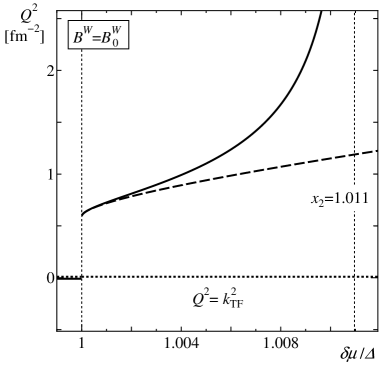
(b)

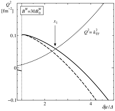
Figure 2: Spatial momentum squared $Q^{2}$ at which the system is most unstable to the gap amplitude variation. The solid lines are the results from Eq. (61), and the dashed lines are the results from Eq. (63). (a) The typical case $\Delta=100\mbox{ MeV}$ and $B^{W}=B^{W}_{0}=50\mbox{ MeV fm}^{5}$. For $1<\delta\mu/\Delta<x_{2}=1.011$, $Q^{2}$ is much larger than $k_{\rm TF}^{2}$ indicating that the system takes a form of the Coulomb lattice with periodicity $\sim 2\pi/Q$. (b) For large $B^{W}=30B^{W}_{0}$ there appears the region in which $Q^{2}$ is smaller than $k_{\rm TF}^{2}$. Then the screening effect is so significant that the system can be phase separated.

Recall that the local thermodynamic potential (46) suggests an even stronger instability due to the variation of the gauge fields. This implies the possibility that the normal state in the mixed phase is replaced by the LOFF state without amplitude oscillations. Near $\delta\mu=\Delta$, $|\delta n_{-}/\delta\Delta|$ is far larger than the typical scale $\mu^{2}/\pi^{2}$ of the density of states, indicating that the gap might remain in the region where the Fermi surface separation between $u$ and $d$ quarks is maximal. Consequently, the LOFF state, which occurs only for nonzero $\Delta$, could appear in such a region.

In Fig. 3, we summarize the instabilities of the homogeneous system with respect to various inhomogeneities and the resultant possible states on the $B^{W}$ versus $\delta\mu/\Delta$ plane. Through the last term in the thermodynamic potential (15), the presence of the gapless modes in the gapless 2SC state underlies all the instabilities but the chromomagnetic instability that occurs also in the 2SC state. It is noteworthy that no LOFF state with amplitude oscillations is expected in the gapless state when $B^{W}$ is larger than the critical value $B^{W}_{c}$. We emphasize that all we can know from the present stability analysis is how the system is driven by infinitesimal variations of the densities and the order parameter. This property, while being suggestive of the final destination of the unstable system, does not tell us what the ground state really is (see Ref. Shov for its candidates).

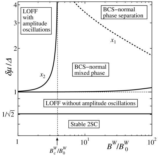
Figure 3: The possible phase structures implied by a stability analysis on the $B^{W}$ versus $\delta\mu/\Delta$ plane. The parameter $B^{W}$ is normalized by a typical value $B^{W}_{0}=50$ MeV fm⁵. The solid line slightly above $\delta\mu/\Delta=1$ represents $v(Q)=0$, while $\delta\mu/\Delta=1$ corresponds to $v_{0}=0$. It is thus obvious that the bulk part $v_{0}$ given by Eq. (56) dominates the behavior of $v(Q)$. The line labeled with $x_{2}$ is determined by the condition $v_{g}=0$ from Eq. (57). The dashed line labeled with $x_{1}$ indicates the criterion $Q^{2}=k_{\rm TF}^{2}$, in the left (right) of which the system tends towards a mixed (separated) state. Note that with increasing $\delta\mu/\Delta$, $x_{2}$ and $x_{1}$ asymptotically approach a critical line, $B^{W}=B^{W}_{c}$, given by Eq. (64) from left and right, respectively.

The results shown in Fig. 3 are in agreement with our intuitive expectation: For larger $B^{W}$ the BCS-normal interface costs a larger energy, meaning that a phase consisting of larger domains is preferable energetically. Therefore the region of the BCS-normal phase separation becomes wider on the phase diagram with increasing $B^{W}$. It should be mentioned that within the present approximation including the energy variations of second order in the inhomogeneities, there is no clear transition between the mixed and separated states; there can be a first order transition between them, whose clarification is beyond the scope of this paper.

Note that we changed $B^{W}$ as a variable parameter, while it is equivalent to changing $\Delta$. This is because the conditions determining $x_{1}$ and $x_{2}$ would not be altered if $\Delta$ is multiplied by an arbitrary factor $\zeta$ and at the same time $B^{W}$ is divided by $\zeta^{2}$. Thus, a larger $B^{W}$ with a fixed $\Delta$ corresponds to a larger $\Delta$ with a fixed $B^{W}$. Since $\Delta$ should not exceed $\Delta_{\rm 2SC}$ (see Fig. 1), however, drastic change in $\Delta$ would not be realistic.

We conclude this section by noting that the density functional (28) was originally written by assuming that ${\bf q}$ is small. If the true value of ${\bf q}$ is large, therefore, one would need extension of the framework by including the higher-order gradient energies. One encounters this situation especially when $\delta\mu/\Delta$ is close to $x_{2}$ as can be seen in Fig. 2.

V Conclusions

We have systematically examined instabilities of the homogeneous and neutral superconducting states for two-flavor quark matter with respect to inhomogeneities in the quark and electron densities and in the phases and amplitude of the order parameter. The result was summarized in Fig. 3. We thus clarified the role of the gapless quark modes, the density and gap gradients, and the electron screening in determining the structure of spontaneous fluctuations.

However, open problems still remain. First, the spatial scale of the possible LOFF states remains to be estimated. This is because this scale is determined by the competition between the negative second-order gradient term and the unknown fourth-order term Hatsuda . Extension to the case of nonzero temperature is significant for possible application to the interiors of compact stars. Since the influence of the gapless quark modes on the thermodynamic potential is smoothed out at nonzero temperature, the instabilities as discussed here are likely to be weakened. Finally, extension to the case of three-flavor quark matter is also important for the description of a more realistic situation. For this purpose, the mean-field analysis of the phase diagram and the chromomagnetic instabilities would be a good starting point.

- (1) B.C. Barrois, Nucl. Phys. B129, 390 (1977).
- (2) D. Bailin and A. Love, Phys. Rep. 107, 325 (1984).
- (3) M. Alford, K. Rajagopal, and F. Wilczek, Nucl. Phys. B537, 443 (1999).
- (4) E. Gubankova, W.V. Liu, and F. Wilczek, Phys. Rev. Lett. 91, 032001 (2003).
- (5) I.A. Shovkovy and M. Huang, Phys. Lett. B 564, 205 (2003); M. Huang and I.A. Shovkovy, Nucl. Phys. A729, 835 (2003).
- (6) M. Alford, C. Kouvaris, and K. Rajagopal, Phys. Rev. Lett. 92, 222001 (2004); Phys. Rev. D 71, 054009 (2005).
- (7) P.F. Bedaque and T. Schäfer, Nucl. Phys. A697, 802 (2002); D.B. Kaplan and S. Reddy, Phys. Rev. D 65, 054042 (2002); A. Kryjevski, D.B. Kaplan, and T. Schäfer, Phys. Rev. D 71, 034004 (2005).
- (8) H. Müther and A. Sedrakian, Phys. Rev. D 67, 085024 (2003).
- (9) M. Huang and I.A. Shovkovy, Phys. Rev. D 70, 051501 (2004); ibid. 094030 (2004).
- (10) R. Casalbuoni, R. Gatto, M. Mannarelli, G. Nardulli, and M. Ruggieri, Phys. Lett. B 605, 362 (2005); 615, 297(E) (2005); M. Alford and Q. h. Wang, J. Phys. G 31, 719 (2005); K. Fukushima, Phys. Rev. D 72, 074002 (2005).
- (11) I. Giannakis and H.-C. Ren, Phys. Lett. B 611, 137 (2005).
- (12) M.M. Forbes, E. Gubankova, W.V. Liu, and F. Wilczek, Phys. Rev. Lett. 94, 017001 (2005).
- (13) See, e.g., I.A. Shovkovy, nucl-th/0511014; M. Ciminale, G. Nardulli, M. Ruggieri, and R. Gatto, Phys. Lett. B 636, 317 (2006).
- (14) P. Fulde and R.A. Ferrell, Phys. Rev. 135, A550 (1964); A.I. Larkin and Yu.N. Ovchinnikov, Zh. Eksp. Teor. Fiz. 47, 1136 (1964) [Sov. Phys. JETP 20, 762 (1965)].
- (15) P.F. Bedaque, H. Caldas, and G. Rupak, Phys. Rev. Lett. 91, 247002 (2003).
- (16) S. Reddy and G. Rupak, Phys. Rev. C 71, 025201 (2005).
- (17) R. Rapp, T. Schäfer, E. Shuryak, and M. Velkovsky, Phys. Rev. Lett. 81, 53 (1998).
- (18) G. Sarma, Phys. Chem. Solid 24, 1029 (1963).
- (19) C.F. von Weizsäcker, Z. Phys. 96, 431 (1935); K.A. Brueckner, J.R. Buchler, S. Jorna, and R.J. Lombard, Phys. Rev. 171, 1188 (1968).
- (20) E. Engel and R.M. Dreizler, Phys. Rev. A 35, 3607 (1987); M. Centelles, X. Viñas, M. Barranco, and P. Schuck, Nucl. Phys. A519, 73c (1990).
- (21) K. Iida and G. Baym, Phys. Rev. D 65, 014022 (2002).
- (22) G.B. Partridge, W. Li, R.I. Kamar, Y.-A. Liao, and R.G. Hulet, Science 311, 503 (2006).
- (23) E.V. Gorbar, M. Hashimoto, and V.A. Miransky, Phys. Rev. Lett. 96, 022005 (2006).
- (24) G. Baym, H. A. Bethe, and C.J. Pethick, Nucl. Phys. A175, 225 (1971); C.J. Pethick, D.G. Ravenhall, and C.P. Lorenz, Nucl. Phy. A584, 675 (1995); G. Watanabe and K. Iida, Phys. Rev. C 68, 045801 (2003).
- (25) T. Hatsuda (private communication).