Bicocca-FT-06-4

KA–TP–03–2006

SFB–CPP–06–10

hep-ph/0603177

Next-to-leading order QCD corrections to $W^{+}W^{-}$ production via
vector-boson fusion

Barbara Jäger¹, Carlo Oleari² and Dieter Zeppenfeld^{1 1} Institut für Theoretische Physik, Universität Karlsruhe, P.O.Box 6980, 76128 Karlsruhe, Germany

² Dipartimento di Fisica ”G. Occhialini”, Università di Milano-Bicocca, 20126 Milano, Italy

Vector-boson fusion processes constitute an important class of reactions at hadron colliders, both for signals and backgrounds of new physics in the electroweak interactions. We consider what is commonly referred to as $W^{+}W^{-}$ production via vector-boson fusion (with subsequent leptonic decay of the $W$s), or, more precisely, $e^{+}\nu_{e}\,\mu^{-}\bar{\nu}_{\mu}$ + 2 jets production in proton-proton scattering, with all resonant and non-resonant Feynman diagrams and spin correlations of the final-state leptons included, in the phase-space regions which are dominated by $t$-channel electroweak-boson exchange. We compute the next-to-leading order QCD corrections to this process, at order $\alpha^{6}\alpha_{s}$. The QCD corrections are modest, changing total cross sections by less than 10%. Remaining scale uncertainties are below 2%. A fully-flexible next-to-leading order partonic Monte Carlo program allows to demonstrate these features for cross sections within typical vector-boson-fusion acceptance cuts. Modest corrections are also found for distributions.

1 Introduction

Vector-boson fusion (VBF) processes form a particularly interesting class of scattering events from which one hopes to gain insight into the dynamics of electroweak symmetry breaking. The most prominent example is Higgs boson production, that is the process $qq\,\mbox{$\rightarrow$}\,qqH$, which can be viewed as quark scattering via $t$-channel exchange of a weak boson, with the Higgs boson radiated off the $W$ or $Z$ propagator. Alternatively, one may view this process as two weak bosons fusing to form the Higgs boson. Higgs boson production via VBF has been studied intensively as a tool for Higgs boson discovery [1, 2] and the measurement of Higgs boson couplings [3] in $pp$ collisions at the CERN Large Hadron Collider (LHC). The two scattered quarks in a VBF process are usually visible as forward jets and greatly help to distinguish these $Hjj$ events from backgrounds.

An important background to Higgs searches at the LHC, in particular to the search for $H\,\mbox{$\rightarrow$}\,W^{+}W^{-}$ decays in VBF production, is caused by continuum $W^{+}W^{-}$ production in VBF. The $qq\,\mbox{$\rightarrow$}\,qq\,W^{+}W^{-}$ process forms an irreducible background in Higgs searches which ranges between 15% and 3.5% of the Higgs signal, for Higgs boson masses between 115 and 160 GeV [4]. In fact, the kinematic distributions of the two tagging jets, the suppression of gluon radiation in the central region (due to the $t$-channel color-singlet exchange nature of the VBF process) and many features of the leptonic final state are identical to the $H\,\mbox{$\rightarrow$}\,W^{+}W^{-}$ signal. When trying to determine Higgs boson couplings, the $qq\,\mbox{$\rightarrow$}\,qq\,W^{+}W^{-}$ cross section must be known precisely, which is achieved by calculating the next-to-leading order (NLO) QCD corrections. Such a calculation becomes more crucial when one contemplates using weak-boson scattering processes, and, more precisely, the absence of strong enhancements in these cross sections, as a probe for the existence of a light Higgs boson [5, 6]. Here the knowledge of NLO QCD corrections is essential in order to distinguish the enhancement from strong weak-boson scattering from possible enhancements due to higher order QCD effects.

In two recent papers, the calculation of the NLO QCD corrections was presented for two simpler vector-boson-fusion processes: the $Hjj$ signal cross section [7] and the cross sections for $Zjj$ and $Wjj$ production [8]. Both calculations were turned into fully-flexible parton-level Monte Carlo programs. We here extend this work and describe the calculation and first results for the NLO QCD corrections to $W^{+}W^{-}jj$ production via VBF.

Weak-boson scattering was first considered in the framework of the effective $W$ approximation, where the incoming weak bosons are treated as on-shell particles [9]. This approximation does not provide a reliable prediction for the kinematical distributions of the forward and backward jets which are the main characteristic of vector boson fusion processes [10]. Calculations of the full $qq\,\mbox{$\rightarrow$}\,qq\,W^{+}W^{-}$ processes, first without $W$ decay [11, 12] and then including the full spin correlations of the $W$ decay products in the narrow-width approximation [13], have been available for more than a decade. Within this latter approximation, also the real gluon emission contributions, i.e. the ${\cal O}(\alpha^{4}\alpha_{s})$ cross sections for the $pp\,\mbox{$\rightarrow$}\,W^{+}W^{-}jjj$ subprocesses, with full spin correlations of the $W$ decay leptons, were determined [14]. Very recently, a partonic-level Monte Carlo for all the processes $q_{1}q_{2}\,\mbox{$\rightarrow$}\,q_{3}q_{4}q_{5}q_{6}l\nu$, with exact matrix elements at ${\cal O}(\alpha^{6})$, has become available [15].

In this paper, we consider the proton-proton scattering process $pp\,\mbox{$\rightarrow$}\,e^{+}\nu_{e}\,\mu^{-}\bar{\nu}_{\mu}\,jj(j)\,X$, with all resonant and non-resonant Feynman diagrams and spin correlations of the final-state leptons included, at order $\alpha^{6}\alpha_{s}$. Since this process is very difficult to detect above QCD backgrounds, except in phase-space regions which are completely dominated by $t$-channel electroweak (EW) boson exchange, we only consider $t$-channel contributions, as explained in Sec. 2.1. In the rest of the paper, we will refer also to this approximated process as EW $W^{+}W^{-}jj$ production. Electroweak gauge invariance requires that, beyond vector-boson scattering graphs, also the direct emission of the produced (virtual) $W$s off the quark lines be considered. Several examples are depicted in Fig. 1, which shows the basic Feynman-graph topologies which need to be considered for our calculation at tree level, for the particular subprocess $uc\,\mbox{$\rightarrow$}\,uc\,e^{+}\nu_{e}\,\mu^{-}\bar{\nu}_{\mu}$. Real emission contributions (including quark-gluon initiated subprocesses) are generated by attaching an external gluon in all possible ways on the two quark lines in Fig. 1. For the virtual corrections, we only need to consider Feynman graphs with a virtual gluon attached to a single quark line: gluon exchange between the up- and the charm-quark line leads to a color-octet state for the external $u\bar{u}$ or $c\bar{c}$ pair, which cannot interfere with the color-singlet structure at tree level. As a result, the virtual contributions contain, at most, pentagon diagrams, which arise e.g. by connecting the incoming and the outgoing up-quark in Fig. 1 (a) with a virtual gluon. The other graphs in Fig. 1 lead to box, vertex, or quark self-energy corrections, and these latter classes have already been encountered in Ref. [8].

Many aspects of the present calculation parallel this previous work. The cancellation of collinear and soft divergences for generic VBF processes was described in detail in Ref. [7] and need not be repeated here, since it can be applied verbatim for the case at hand. The calculation of vertex and box corrections was needed for the case of $W$ and $Z$ production [8] already, and, thus, these aspects of the virtual corrections need a brief review only. This review is provided in Sec. 2, where we describe the details of our calculation and the approximations with regard to crossed diagrams in the presence of identical quark flavors. As in the previous work, we regularize the loop integrals via dimensional reduction and separate the virtual amplitudes into $1/\epsilon^{2}$ and $1/\epsilon$ terms, which multiply the Born amplitude, and remaining finite terms, which are then calculated numerically, using the helicity-amplitude techniques of Ref. [16]. A major concern here is the numerically stable and fast evaluation of the pentagon graphs. We make use of Ward identities and map large fractions of the pentagon contributions onto more easily evaluable four-point functions. Another important feature is the systematic use of “leptonic tensors” which describe groups of purely electroweak subdiagrams.

In Section 3, we describe the numerous consistency tests which we have performed, ranging from comparison to code generated by MadGraph [17] for the tree-level amplitudes to gauge invariance tests. In addition, we present the properties of our numerical Monte Carlo program and how we have dealt with the gauge invariant handling of finite $W/Z$ widths, the singularities for incoming photons and the choice of physical parameters. We then use this Monte Carlo program to produce first results for EW $W^{+}W^{-}jj$ production at the LHC. Of particular concern is the scale dependence of the NLO results, which provides an estimate for the residual theoretical error of our cross-section calculations. We discuss the scale dependence and the size of the radiative corrections for various distributions in Sec. 4. Conclusions are given in Sec. 5.

Figure 1: The six Feynman-graph topologies contributing to the Born process $uc\,\mbox{$\rightarrow$}\,uc\,e^{+}\nu_{e}\,\mu^{-}\bar{\nu}_{\mu}$, a template for neutral-current processes. Diagrams analogous to (a), (b), (e) and (f), with vector-boson emission off the lower quark line, are not shown.

2 Elements of the calculation

Our goal is the calculation of EW $W^{+}W^{-}jj$ production cross sections with NLO QCD accuracy in phase-space regions which are typical for vector-boson fusion. This implies that some electroweak contributions, like triple gauge boson production ($pp\mbox{$\rightarrow$}W^{+}W^{-}V$ with $V\mbox{$\rightarrow$}jj$), can safely be neglected. These approximations will be specified below. Also, we make use of the general structure of NLO QCD corrections to VBF processes: it is sufficient to specify the contributions to the Born, the real-radiation and virtual amplitudes which enter the cross section expressions of Ref. [7]. In this section, we describe how these contributions have been computed, the approximations used throughout this calculation and some technical details.

2.1 Tree-level contribution and approximations

The Feynman diagrams contributing to $pp\,\mbox{$\rightarrow$}\,jj\,e^{+}\nu_{e}\,\mu^{-}\bar{\nu}_{\mu}$, where both resonant and non-resonant processes are fully considered, can be grouped into six separate classes. The first group of two, which consists of the VBF processes considered in this paper, is characterized by $t$-channel neutral-current (NC) and charged-current (CC) exchange between the two scattering quark lines. The other four classes correspond to $u$- and $s$-channel exchange. The NC and CC labels are assigned depending on the external quark flavors: the incoming and outgoing quark charges on each quark line coincide for a neutral current process and differ by one unit of $|e|$ for a charged current process.

For each neutral-current process, and in the unitary gauge which we use throughout, there are 181 Feynman graphs, which can be grouped into six distinct topologies. Generic diagrams for each of the topologies (a) to (f) are shown in Fig. 1 for the specific subprocess $uc\,\mbox{$\rightarrow$}\,uc\,e^{+}\nu_{e}\,\mu^{-}\bar{\nu}_{\mu}$. They correspond to the following configurations:

• Two virtual $W$ bosons are emitted from the same quark line and in turn decay leptonically.

• A virtual $\gamma$ or $Z$ boson ($V$) with subsequent leptonic decay is emitted from either quark line. The tree-level expression for the sub-amplitude $V\,\mbox{$\rightarrow$}\,e^{+}\nu_{e}\,\mu^{-}\bar{\nu}_{\mu}$ is given by the tensor $\Gamma_{V}^{\alpha}$, where $\alpha$ is the tensor index carried by the vector boson.

• The leptonically-decaying $W$ bosons are emitted from two different quark lines.

• Vector-boson fusion in the $t$-channel gives rise to the sub-amplitude $VV\,\mbox{$\rightarrow$}\,e^{+}\nu_{e}\,\mu^{-}\bar{\nu}_{\mu}$, which is characterized by the tensor $T_{VV}^{\alpha\beta}$. The tensor indices of the scattering $V$ bosons are indicated with $\alpha$ and $\beta$.

• The leptons are produced by an external $W^{-}$ boson emitted from a quark line and a $W^{+}V\,\mbox{$\rightarrow$}\,e^{+}\nu_{e}$ fusion process in the $t$-channel. The latter is described by $T_{W^{+}V}^{\alpha\beta}$.

• The leptons stem from $W^{+}$ emission from a quark line, accompanied by $t$-channel $W^{-}V\,\mbox{$\rightarrow$}\,\mu^{-}\bar{\nu}_{\mu}$ scattering, described by $T_{W^{-}V}^{\alpha\beta}$.

The propagator factors $1/(q^{2}-m_{V}^{2}+im_{V}\Gamma_{V})$ are included in the definitions of the sub-amplitudes introduced above, which we call “leptonic tensors” in the following.

Figure 2: Diagrams contributing to the scattering amplitude $T_{W^{+}V}^{\alpha\beta}$, depicted in Fig. 1 (e), that describe the tree-level subprocess $W^{+}V\mbox{$\rightarrow$}e^{+}\nu_{e}$, where $V$ is a $\gamma$ or a $Z$ vector boson, and $\alpha$ and $\beta$ are the tensor indices carried by the charged and neutral vector bosons, respectively.

The explicit structure of one of these leptonic tensors is given in Fig. 2, where we have plotted the Feynman diagrams contributing to $T_{W^{+}V}^{\alpha\beta}$: a virtual $W^{+}$ and a virtual $\gamma$ or $Z$ fuse into a final state $e^{+}\nu_{e}$ lepton pair, and the sub-amplitude corresponding to these three graphs is the leptonic tensor $T^{\alpha\beta}_{W^{+}V}$ which appears in graphs like Fig. 1 (e).

For each charged-current process, such as $us\,\mbox{$\rightarrow$}\,dc\,e^{+}\nu_{e}\,\mu^{-}\bar{\nu}_{\mu}$ or $dc\,\mbox{$\rightarrow$}\,us\,e^{+}\nu_{e}\,\mu^{-}\bar{\nu}_{\mu}$, there are 92 Feynman graphs. The different topologies are completely analogous to the ones for neutral current processes: simply interchange the $t$-channel bosons $\gamma,Z\leftrightarrow W$ in Fig. 1. The only new tensor structure that occurs is $T_{W^{+}W^{-}}^{\alpha\beta}$, which describes the sub-amplitude for $W^{+}W^{-}\,\mbox{$\rightarrow$}\,e^{+}\nu_{e}\,\mu^{-}\bar{\nu}_{\mu}$. The corresponding Feynman graph topology is depicted in Fig. 3.

Figure 3: Contribution from $W^{+}W^{-}$ fusion to the scattering process $us\,\mbox{$\rightarrow$}\,dc\,e^{+}\nu_{e}\,\mu^{-}\bar{\nu}_{\mu}$. The tensor $T_{W^{+}W^{-}}^{\alpha\beta}$ contains all the tree-level diagrams contributing to the process $W^{+}W^{-}\,\mbox{$\rightarrow$}\,e^{+}\nu_{e}\,\mu^{-}\bar{\nu}_{\mu}$, where $\alpha$ and $\beta$ are the tensor indices carried by the $W^{+}$ and $W^{-}$ vector bosons, respectively.

By crossing the external quark lines, one either obtains anti-quark initiated $t$-channel processes like $\bar{u}c\mbox{$\rightarrow$}\bar{u}c\,e^{+}\nu_{e}\,\mu^{-}\bar{\nu}_{\mu}$ (which we fully take into account in our calculation) or one arrives at NC or CC $s$- or $u$-channel exchange between the two quark lines, which we count as the other four classes of $jje^{+}\nu_{e}\,\mu^{-}\bar{\nu}_{\mu}$ processes:

• $s$-channel exchange leads to diagrams where all the virtual vector bosons are time-like. They correspond to diagrams called conversion, Abelian and non-Abelian annihilation in Ref. [18], and contain vector-boson production with subsequent decay into pairs of fermions.

• $u$-channel exchange occurs for diagrams obtained by interchange of identical initial- or final-state (anti)quarks, such as in the $uu\,\mbox{$\rightarrow$}\,uu\,e^{+}\nu_{e}\,\mu^{-}\bar{\nu}_{\mu}$ subprocess.

In our calculation, we have neglected contributions from $s$-channel exchange completely. In addition, any interference effects of $t$-channel and $u$-channel diagrams are neglected. This is justified because, in the phase-space region where VBF can be observed experimentally, with widely-separated quark jets of very large invariant mass, the neglected terms are strongly suppressed by large momentum transfer in one or more weak-boson propagators. Color suppression further reduces any interference terms. In Ref. [8] we have checked that, for the analogous process $pp\,\mbox{$\rightarrow$}\,W/Z\,jj$, the contribution from the two neglected classes and from interference effects accounts for less than 0.3% of the total cross section, at leading order. Since we expect QCD corrections to the neglected terms to be modest, the above approximations are fully justified within the accuracy of our NLO calculation.

2.2 Real corrections

The real-emission corrections to EW $W^{+}W^{-}jj$ production with a gluon in the final state are obtained by attaching one gluon to the quark lines in all possible ways. There are 836 graphs in the case of neutral-current processes and 444 for the charged-current ones.

The contributions with an initial-state gluon are obtained by crossing the previous diagrams, promoting the final-state gluon as incoming parton, and an initial-state (anti-)quark as final-state particle. We again remove all diagrams where all electroweak boson propagators are time-like. Such diagrams, for consistency, must be removed since we have not considered the corresponding Born contributions, namely the $s$-channel diagrams corresponding to triple weak-boson production. These diagrams are strongly suppressed when VBF cuts (see Sec. 4) are applied to the final-state jets.

In the regions of phase space where soft and collinear configurations can occur, we encounter singularities in the phase-space integrals of the real-emission squared amplitudes. The regularization of these singularities in the dimensional-regularization scheme, with space-time dimension $d=4-2\epsilon$, and the counter-terms which are needed to get finite expressions within the subtraction method, are discussed extensively in the literature (see, for example, [19]). Since these divergences only depend on the color structure of the external partons, the subtraction terms encountered for EW $W^{+}W^{-}jj$ production are identical in form to those found for Higgs boson production in VBF [7] and for EW $Vjj$ production [8]. The integration over the singular counter-terms yields, after factorization of the parton distribution function, the contribution

$$<{\boldsymbol{I}}(\epsilon)>=|{\cal M}_{B}|^{2}\frac{\alpha_{s}(\mu_{R})}{2\pi}C_{F}\left(\frac{4\pi\mu_{R}^{2}}{Q^{2}}\right)^{\epsilon}\Gamma(1+\epsilon)\left[\frac{2}{\epsilon^{2}}+\frac{3}{\epsilon}+9-\frac{4}{3}\pi^{2}\right]\;.$$ (2.1)

Here, the notation of Ref. [19], but adapted to dimensional reduction, has been used. ${\cal M}_{B}$ denotes the amplitude of the corresponding Born process and $Q^{2}$ is the momentum transfer between the initial and final state quark in Fig. 1. These singular terms are eventually cancelled by the virtual corrections, when infrared-safe quantities are computed.

2.3 Virtual corrections

As for the real-radiation cross sections, the divergences that affect the virtual gluon contributions depend on the color structure of the external partons. The main difference with $Hjj$ and $Vjj$ production is that the finite parts of the virtual corrections are more complicated for the present case, since the previous two processes only sport vertex and box corrections, while now we have to deal with pentagon-type loop integrals.

The QCD corrections to EW $W^{+}W^{-}jj$ production appear as two gauge-invariant subsets, corresponding to gluon emission and reabsorption on either the upper or the lower fermion line in Fig. 1. Due to the color-singlet nature of the exchanged electroweak bosons, any interference terms of the Born amplitude with virtual sub-amplitudes with gluons attached to both the upper and the lower quark lines vanish identically at order $\alpha_{s}$. Hence, it is sufficient to consider radiative corrections to a single quark line only, which we here take as the upper one. Corrections to the lower fermion line are an exact copy. We have regularized the virtual corrections in the dimensional reduction scheme [20]: we have performed the Passarino-Veltman (PV) [21] reduction of the tensor integrals in $d=4-2\epsilon$ dimensions, while the algebra of the Dirac gamma matrices, of the external momenta and of the polarization vectors has been performed in $d=4$ dimensions.

We split the virtual corrections into three classes: the virtual corrections along a quark line with only one vector boson attached (e.g. diagram (d) in Fig. 1 or diagrams (a), (b), (e) and (f) when considering corrections to the lower quark line), the virtual corrections along a quark line with two vector bosons attached (e.g. diagrams (b), (c), (e), (f)), and the virtual corrections along a quark line with three vector bosons attached (e.g. diagram (a)).

I. The virtual NLO QCD contribution to any tree-level Feynman amplitude ${\cal M}_{B}^{(i)}$ which has a single electroweak boson $V_{1}$ (of momentum $q_{1}$) attached to a quark line,

$$q(k_{1})\,\mbox{$\rightarrow$}\,q(k_{2})+V_{1}(q_{1})\,,$$ (2.2)

is factorizable in terms of the amplitude for the corresponding Born graph

$${\cal M}_{V}^{(i)}={\cal M}_{B}^{(i)}\,\frac{\alpha_{s}(\mu_{R})}{4\pi}\,C_{F}\left(\frac{4\pi\mu_{R}^{2}}{Q^{2}}\right)^{\epsilon}\Gamma(1+\epsilon)\left[-\frac{2}{\epsilon^{2}}-\frac{3}{\epsilon}+c_{\rm virt}+{\cal O}\left(\epsilon\right)\right]\,.$$ (2.3)

Here $\mu_{R}$ is the renormalization scale, and the boson virtuality $Q^{2}=-(k_{1}-k_{2})^{2}$ is the only relevant scale in the process, since the quarks are assumed to be massless, $k_{1}^{2}=k_{2}^{2}=0$. In dimensional reduction, the finite contribution $c_{\rm virt}$ is equal to $\pi^{2}/3-7$ ($c_{\rm virt}=\pi^{2}/3-8$ in conventional dimensional regularization).

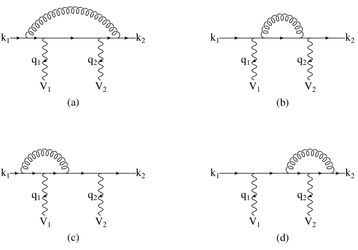
Figure 4: Virtual corrections for a fermion line with two attached vector bosons, $V_{1}(q_{1})$ and $V_{2}(q_{2})$. The finite part of the sum of these graphs defines the reduced amplitude $\widetilde{\cal M}_{V_{1}V_{2},\tau}\left(q_{1},q_{2}\right)$ of Eq. (2.5).

II. The virtual QCD corrections to the Feynman graphs, where two electroweak bosons $V_{1}$ and $V_{2}$ (of outgoing momenta $q_{1}$ and $q_{2}$) are attached to a quark line, are depicted in Fig. 4. It suffices to consider one of the two possible permutations of $V_{1}$ and $V_{2}$, with kinematics

$$q(k_{1})\,\mbox{$\rightarrow$}\,q(k_{2})+V_{1}(q_{1})+V_{2}(q_{2})\,.$$ (2.4)

Due to the trivial color structure of the tree-level diagram, the divergent part (soft and collinear singularities) of the sum of the four diagrams in Fig. 4 is a multiple of the corresponding Feynman graph at Born level, just like for the vertex corrections,

$${\cal M}_{V}^{(i)} = {\cal M}_{B}^{(i)}\,\frac{\alpha_{s}(\mu_{R})}{4\pi}\,C_{F}\left(\frac{4\pi\mu_{R}^{2}}{Q^{2}}\right)^{\epsilon}\Gamma(1+\epsilon)\left[-\frac{2}{\epsilon^{2}}-\frac{3}{\epsilon}+c_{\rm virt}\right]$$ (2.5)

$$+ \frac{\alpha_{s}(\mu_{R})}{4\pi}\,C_{F}\,\widetilde{\cal M}_{V_{1}V_{2},\tau}^{(i)}\left(q_{1},q_{2}\right)\,e^{2}\,g_{\tau}^{V_{1}f_{1}}g_{\tau}^{V_{2}f_{2}}+{\cal O}(\epsilon)\,.$$

where we define $Q^{2}=2\,k_{1}\cdot k_{2}$, in order to use the same notation as in Eq. (2.3). Here $\tau$ denotes the quark chirality and the electroweak couplings $g_{\tau}^{Vf}$ follow the notation of Ref. [16], with, e.g., $g_{\pm}^{\gamma f}=Q_{f}$, the fermion electric charge in units of $|e|$, $g_{-}^{Wf}=1/(\sqrt{2}\sin\theta_{W})$ and $g_{-}^{Zf}=(T_{3f}-Q_{f}\sin^{2}\theta_{W})/(\sin\theta_{W}\cos\theta_{W})$, where $\theta_{W}$ is the weak mixing angle and $T_{3f}$ is the third component of the isospin of the (left-handed) fermions.

A finite contribution of the virtual diagrams, which is proportional to the Born amplitude (the $c_{\rm virt}$ term), is pulled out in correspondence with Eq. (2.3). The remaining non-universal term, $\widetilde{\cal M}_{V_{1}V_{2},\tau}^{(i)}\left(q_{1},q_{2}\right)$, is also finite and can be expressed in terms of the finite parts of the Passarino-Veltman $B_{ij}$, $C_{ij}$ and $D_{ij}$ functions. The corresponding analytic expressions were given in Ref. [8]. Note that the effective polarization vectors for the electroweak bosons $V_{1}$ and $V_{2}$, which enter the expressions for the $\widetilde{\cal M}_{V_{1}V_{2},\tau}^{(i)}\left(q_{1},q_{2}\right)$, are $W^{\pm}$ decay currents, the leptonic tensors $\Gamma_{V}^{\mu}$ (for Fig. 1 (b)) and/or the entire lower parts of the Feynman graphs for Fig. 1 (c,e,f), when combining Feynman graphs with identical topology.

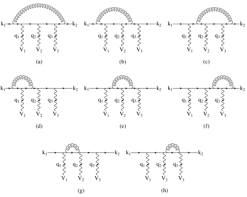
Figure 5: Virtual corrections for a fermion line with three attached vector bosons, $V_{1}(q_{1})$, $V_{2}(q_{2})$ and $V_{3}(q_{3})$. The finite part of the sum of these graphs defines the reduced amplitude $\widetilde{\cal M}_{V_{1}V_{2}V_{3},\tau}\left(q_{1},q_{2},q_{3}\right)$ of Eq. (2.7).

III. The virtual QCD corrections to the Feynman graphs where three electroweak bosons $V_{1}$, $V_{2}$ and $V_{3}$ (of outgoing momenta $q_{1}$, $q_{2}$ and $q_{3}$) are attached to a quark line, are depicted in Fig. 5. It suffices to consider one of the six possible permutations of $V_{1}$, $V_{2}$ and $V_{3}$, with kinematics

$$q(k_{1})\,\mbox{$\rightarrow$}\,q(k_{2})+V_{1}(q_{1})+V_{2}(q_{2})+V_{3}(q_{3})\,.$$ (2.6)

The trivial color structure of the tree-level diagram allows the factorization of the divergent part of the sum of the eight diagrams in Fig. 5 in terms of the corresponding Born sub-amplitude

$${\cal M}_{V}^{(i)} = {\cal M}_{B}^{(i)}\,\frac{\alpha_{s}(\mu_{R})}{4\pi}\,C_{F}\left(\frac{4\pi\mu_{R}^{2}}{Q^{2}}\right)^{\epsilon}\Gamma(1+\epsilon)\left[-\frac{2}{\epsilon^{2}}-\frac{3}{\epsilon}+c_{\rm virt}\right]$$ (2.7)

$$+ \frac{\alpha_{s}(\mu_{R})}{4\pi}\,C_{F}\,\widetilde{\cal M}_{V_{1}V_{2}V_{3},\tau}^{(i)}\left(q_{1},q_{2},q_{3}\right)\,e^{3}\,g_{\tau}^{V_{1}f_{1}}g_{\tau}^{V_{2}f_{2}}g_{\tau}^{V_{3}f_{3}}+{\cal O}(\epsilon)\,.$$

Again, a finite contribution from the virtual diagrams, proportional to the Born amplitude ($c_{\rm virt}$), is pulled out and the remaining finite part is indicated with $\widetilde{\cal M}_{V_{1}V_{2}V_{3},\tau}^{(i)}\left(q_{1},q_{2},q_{3}\right)$.

The factorization of the divergent parts of the various virtual contributions, as multiples of the corresponding Feynman amplitudes at Born level, ${\cal M}_{B}^{(i)}$, implies that the overall infrared and collinear divergences multiply the complete Born amplitude, ${\cal M}_{B}=\sum_{i}{\cal M}_{B}^{(i)}$. We can summarize our results for the virtual corrections to the individual fermion lines by writing the complete virtual amplitude ${\cal M}_{V}$ as

$${\cal M}_{V} = {\cal M}_{B}\,\frac{\alpha_{s}(\mu_{R})}{4\pi}\,C_{F}\left(\frac{4\pi\mu_{R}^{2}}{Q^{2}}\right)^{\epsilon}\Gamma(1+\epsilon)\left[-\frac{2}{\epsilon^{2}}-\frac{3}{\epsilon}+c_{\rm virt}\right]$$ (2.8)

$$+ \frac{\alpha_{s}(\mu_{R})}{4\pi}\,C_{F}\,e^{2}\sum_{i}\widetilde{\cal M}_{V_{1}V_{2},\tau}^{(i)}\left(q_{1},q_{2}\right)g_{\tau}^{V_{1}f_{1}}g_{\tau}^{V_{2}f_{2}}$$

$$+ \frac{\alpha_{s}(\mu_{R})}{4\pi}\,C_{F}\,e^{3}\sum_{i}\widetilde{\cal M}_{V_{1}V_{2}V_{3},\tau}^{(i)}\left(q_{1},q_{2},q_{3}\right)g_{\tau}^{V_{1}f_{1}}g_{\tau}^{V_{2}f_{2}}g_{\tau}^{V_{3}f_{3}}+{\cal O}(\epsilon)$$

$$= {\cal M}_{B}\,\frac{\alpha_{s}(\mu_{R})}{4\pi}\,C_{F}\left(\frac{4\pi\mu_{R}^{2}}{Q^{2}}\right)^{\epsilon}\Gamma(1+\epsilon)\left[-\frac{2}{\epsilon^{2}}-\frac{3}{\epsilon}+c_{\rm virt}\right]+\widetilde{\cal M}_{V}\,,$$

where the sums run over the different orderings of the attached weak bosons and the relevant topologies of Fig. 1, when using effective polarization vectors for the electroweak bosons, as discussed below Eq. (2.5). Note that $\widetilde{\cal M}_{V}$ is completely finite. The NLO contribution to the cross section at order $\alpha_{s}$ comes from the interference of the virtual amplitude with the Born term. For corrections to a quark line it is given by

$$2\mathop{\rm Re}\left[{\cal M}_{V}{\cal M}_{B}^{*}\right]=|{\cal M}_{B}|^{2}\frac{\alpha_{s}(\mu_{R})}{2\pi}C_{F}\left(\frac{4\pi\mu_{R}^{2}}{Q^{2}}\right)^{\epsilon}\Gamma(1+\epsilon)\left[-\frac{2}{\epsilon^{2}}-\frac{3}{\epsilon}+c_{\rm virt}\right]\ +2\mathop{\rm Re}\left[\widetilde{\cal M}_{V}{\cal M}_{B}^{*}\right]\,.$$ (2.9)

The divergent piece appears as a multiple of the Born amplitude squared and it cancels explicitly against the phase-space integral of the dipole terms (see Ref. [19] and Eq. (2.10) of Ref. [7])

$$<{\boldsymbol{I}}(\epsilon)>=|{\cal M}_{B}|^{2}\frac{\alpha_{s}(\mu_{R})}{2\pi}C_{F}\left(\frac{4\pi\mu_{R}^{2}}{Q^{2}}\right)^{\epsilon}\Gamma(1+\epsilon)\left[\frac{2}{\epsilon^{2}}+\frac{3}{\epsilon}+9-\frac{4}{3}\pi^{2}\right]\,,$$ (2.10)

which absorbs the real-emission singularities which are left after factorization of the parton distribution functions. After this cancellation, all the remaining integrals are finite and can, hence, be evaluated in $d=4$ dimensions.

2.4 Technical details

Our Monte Carlo program computes all amplitudes numerically, using the helicity technique and the formalism of Ref. [16]. For the tree-level and real-emission amplitudes (including counter-terms), the method is straightforward, since these contributions are finite at each phase-space point. The evaluation of the helicity amplitudes is very fast, due to the modular structure that one achieves by grouping the whole set of diagrams according to the topologies illustrated in Fig. 1. The $W^{+}\mbox{$\rightarrow$}e^{+}\nu_{e}$ and $W^{-}\mbox{$\rightarrow$}\mu^{-}\bar{\nu}_{\mu}$ decay amplitudes and the single index leptonic tensors $\Gamma_{V}^{\alpha}$ ($V=Z,\;\gamma$) are effective polarization vectors which only depend on the lepton momenta. They are the same for all subprocesses, i.e. they do not depend on quark flavor or whether quarks and/or anti-quarks scatter. Similarly the second-rank leptonic tensors $T_{VV}^{\alpha\beta}$, $T_{W^{\pm}V}^{\alpha\beta}$ and $T_{W^{+}W^{-}}^{\alpha\beta}$ are independent of quark flavor and come in just two kinematic configurations, depending on whether or not an external gluon is attached to the upper or the lower quark line in Fig. 1. Correspondingly, the leptonic tensors are calculated first in our numerical program and then used in crossed subprocesses and subtraction terms. The code for these leptonic tensors has been generated with MadGraph and adapted to the tensor structure required for our full program. We note, in passing, that this approach allows for straightforward inclusion of new physics effects in the electroweak sector: only the leptonic tensors would be affected by modifications like anomalous three- or four-gauge-boson couplings or strong electroweak-boson scattering. One major advantage of the modular strategy is the increase in computational speed. In the calculation of the real-emission contributions, which constitute the most CPU-time intensive part of the code, our program is about 70 times faster than a direct use of MadGraph-generated routines for the individual subprocesses.

Special care has to be taken in the extraction of the finite parts $\widetilde{\cal M}_{V_{1}V_{2},\tau}\left(q_{1},q_{2}\right)$ and $\widetilde{\cal M}_{V_{1}V_{2}V_{3},\tau}\left(q_{1},q_{2},q_{3}\right)$, which are contained in the full virtual amplitude of Eq. (2.8). In order to keep the expressions small and fast to evaluate, we have implemented the PV tensor reduction numerically. Here we are adopting a natural extension of the PV notation, and we call $E_{ij}$ the coefficient functions from the tensor reduction of pentagon integrals. Since the finite $\widetilde{\cal M}_{V_{1}V_{2},\tau}\left(q_{1},q_{2}\right)$ and $\widetilde{\cal M}_{V_{1}V_{2}V_{3},\tau}\left(q_{1},q_{2},q_{3}\right)$ virtual sub-amplitudes only contain the finite pieces of the various tensor integrals, one needs to track how the divergent contributions in the expressions of the scalar integrals feed into the expressions of the tensor coefficients $B_{ij}$, $C_{ij}$, $D_{ij}$ and $E_{ij}$, and how they generate finite contributions in coefficients that contain a factor $(d-4)$ in the numerator. The resulting analytical expression for $\widetilde{\cal M}_{V_{1}V_{2},\tau}\left(q_{1},q_{2}\right)$, in terms of finite functions, is given in Ref. [8]. We postpone to a future paper [22] any further technical discussion about the computation of $\widetilde{\cal M}_{V_{1}V_{2}V_{3},\tau}\left(q_{1},q_{2},q_{3}\right)$.

3 Checks and implementation in a parton-level Monte Carlo

The cross-section contributions discussed in the previous section have been implemented in a fully-flexible parton-level Monte Carlo, which is very similar to the programs for $Hjj$ and $Vjj$ production in VBF as described in Refs. [7] and [8]. The matrix-element calculation is divided into three main parts, that deal with the evaluation of the tree-level, the real-emission and the virtual contributions. All elements have been extensively tested as detailed below.

Tree-level contribution
We have compared our tree-level code with purely MadGraph generated output, and we have found agreement with a typical relative accuracy of $10^{-10}$.

Real-radiation contribution
The same comparison has been performed for the real radiation contributions, with typical agreement at the $10^{-10}$ level. In addition, we have also checked the QCD gauge invariance of the real-emission corrections. More specifically, the real-emission amplitude for the process $qq^{\prime}\mbox{$\rightarrow$}qq^{\prime}g\,\,e^{+}\nu_{e}\,\mu^{-}\bar{\nu}_{\mu}$ has the form

$$\mathcal{M}_{R}=\varepsilon_{\mu}(p)\,\mathcal{M}^{\mu}_{R}\,,$$ (3.1)

where $p$ is the momentum of the emitted gluon and $\varepsilon_{\mu}(p)$ its polarization vector. Gauge invariance demands that the amplitude $\mathcal{M}_{R}$ remains unchanged upon the substitution $\varepsilon_{\mu}(p)\,\mbox{$\rightarrow$}$ $\varepsilon_{\mu}(p)+\beta p_{\mu}$ (with $\beta$ arbitrary), that is

$$p_{\mu}\mathcal{M}^{\mu}_{R}=0.$$ (3.2)

This relation is satisfied within the numerical accuracy of the program.

Virtual contribution: code checks
As far as the virtual contribution is concerned, we have implemented two different codes, one analytical, in MAPLE, and one numerical, in fortran. The analytical code sums all the eight Feynman diagrams in Fig. 5, which we call $\mathcal{P}_{\mu_{1}\mu_{2}\mu_{3}}$ for uncontracted polarization vectors of the three electroweak bosons, and writes it in terms of the PV coefficient functions, $B_{ij},\ldots E_{ij}$, in $d$ dimensions. We schematically represent this tensor reduction by

$$\mathcal{P}_{\mu_{1}\mu_{2}\mu_{3}}(k_{1},q_{1},q_{2},q_{3})=\sum_{ij}\,T^{(ij)}_{\mu_{1}\mu_{2}\mu_{3}}\,{\rm(PV)}_{ij}\,,$$ (3.3)

where ${\rm(PV)}_{ij}=\{B_{ij},C_{ij},D_{ij},E_{ij}\}$ is one of the Passarino-Veltman coefficient functions, and the (finite) tensors $T^{(ij)}_{\mu_{1}\mu_{2}\mu_{3}}$ correspond to spinor products describing the quark lines in Fig. 5. The $\mathcal{P}_{\mu_{1}\mu_{2}\mu_{3}}$ and the $(PV)_{ij}$ still contain divergent contributions. We denote their finite parts by $\tilde{\mathcal{P}}_{\mu_{1}\mu_{2}\mu_{3}}$, $\tilde{B}_{ij},\;\tilde{C}_{ij},\;\tilde{D}_{ij},\;\tilde{E}_{ij}$, respectively.

The analytic code contains all the recursion relations that can be used to reduce the PV coefficient functions to combinations of scalar integrals only: $B_{0},C_{0},D_{0}$ and $E_{0}$ functions. The $E_{0}$ function can be further expressed in terms of the sum of five $D_{0}$ functions, as described in Ref. [23], when $d=4-2\epsilon$, in the limit $\epsilon\,\mbox{$\rightarrow$}\,0$. The analytic continuation of $D_{0}$ functions was checked against Ref. [24]. The tensor reduction down to scalar integrals, and the direct substitution of the corresponding expressions computed in $d=4-2\epsilon$ dimensions have been used to check the structure of the divergent terms, and to show that, once contracted with the Born amplitude, they are given by Eq. (2.8).

The expression of $\tilde{\mathcal{P}}_{\mu_{1}\mu_{2}\mu_{3}}$ in terms of PV coefficient functions is turned by MAPLE into a fortran code, where care is taken to obtain the correct limit when $d\,\mbox{$\rightarrow$}\,4$. All the technical details about this part of the program will be given in Ref. [22].

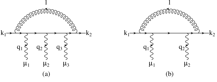
Figure 6: $\mathcal{E}_{\mu_{1}\mu_{2}\mu_{3}}(k_{1},q_{1},q_{2},q_{3})$ and $\mathcal{D}_{\mu_{1}\mu_{2}}(k_{1},q_{1},q_{2})$ of Eqs. (3.4)–(3.7).

Both the analytical and the fortran code have been checked extensively using gauge invariance, applied at different levels of complication:

• at the level of the single pentagon loop (diagram (a) of Fig. 6),

• at the level of the sum of all the virtual corrections along a single quark line, $\mathcal{P}_{\mu_{1}\mu_{2}\mu_{3}}$,

• and at the level of the entire scattering process (for the fortran code).

To illustrate an example of gauge check, we consider the simpler case of the pentagon loop of diagram (a) in Fig. 6

$$\mathcal{E}_{\mu_{1}\mu_{2}\mu_{3}}(k_{1},q_{1},q_{2},q_{3})\equiv\!\!\int\!\!\frac{d^{d}l}{(2\pi)^{d}}\gamma^{\alpha}\frac{1}{l\hskip-3.18057pt\hbox to3.18057pt{\hss$/$\hss}+k\hskip-5.52084pt\hbox to5.52084pt{\hss$/$\hss}_{1}+q\hskip-4.8229pt\hbox to4.8229pt{\hss$/$\hss}_{123}}\gamma_{\mu_{3}}\frac{1}{l\hskip-3.18057pt\hbox to3.18057pt{\hss$/$\hss}+k\hskip-5.52084pt\hbox to5.52084pt{\hss$/$\hss}_{1}+q\hskip-4.8229pt\hbox to4.8229pt{\hss$/$\hss}_{12}}\gamma_{\mu_{2}}\frac{1}{l\hskip-3.18057pt\hbox to3.18057pt{\hss$/$\hss}+k\hskip-5.52084pt\hbox to5.52084pt{\hss$/$\hss}_{1}+q\hskip-4.8229pt\hbox to4.8229pt{\hss$/$\hss}_{1}}\gamma_{\mu_{1}}\frac{1}{l\hskip-3.18057pt\hbox to3.18057pt{\hss$/$\hss}+k\hskip-5.52084pt\hbox to5.52084pt{\hss$/$\hss}_{1}}\gamma_{\alpha}\frac{1}{l^{2}}\,,$$ (3.4)

where $q_{12}=q_{1}+q_{2}$, $q_{123}=q_{1}+q_{2}+q_{3}$, $k_{2}=q_{123}+k_{1}$. Gauge invariance is simply the statement that, upon contracting any one tensor index with the corresponding momentum, and expressing the contracted gamma matrix as the difference of the two adjacent fermionic propagators, the pentagon can be reduced to box integrals $\mathcal{D}_{\mu\nu}$ (see diagram (b) in Fig. 6)

$$q_{1}^{\mu_{1}}\mathcal{E}_{\mu_{1}\mu_{2}\mu_{3}}(k_{1},q_{1},q_{2},q_{3}) = \mathcal{D}_{\mu_{2}\mu_{3}}(k_{1},q_{1}+q_{2},q_{3})-\mathcal{D}_{\mu_{2}\mu_{3}}(k_{1}+q_{1},q_{2},q_{3})\,,$$ (3.5)

$$q_{2}^{\mu_{2}}\mathcal{E}_{\mu_{1}\mu_{2}\mu_{3}}(k_{1},q_{1},q_{2},q_{3}) = \mathcal{D}_{\mu_{1}\mu_{3}}(k_{1},q_{1},q_{2}+q_{3})-\mathcal{D}_{\mu_{1}\mu_{3}}(k_{1},q_{1}+q_{2},q_{3})\,,$$ (3.6)

$$q_{3}^{\mu_{3}}\mathcal{E}_{\mu_{1}\mu_{2}\mu_{3}}(k_{1},q_{1},q_{2},q_{3}) = \mathcal{D}_{\mu_{1}\mu_{2}}(k_{1},q_{1},q_{2})-\mathcal{D}_{\mu_{1}\mu_{2}}(k_{1},q_{1},q_{2}+q_{3})\,.$$ (3.7)

Using the PV tensor reduction, we can express $\mathcal{E}_{\mu_{1}\mu_{2}\mu_{3}}$ as a sum of coefficient functions up to $E_{ij}$ (see Eq. (3.3)), and $\mathcal{D}_{\mu\nu}$ as sum of coefficient functions up to $D_{ij}$, and generate the corresponding fortran code for their finite parts. We can then check that the analytic or numeric expression for $\tilde{\mathcal{E}}_{\mu_{1}\mu_{2}\mu_{3}}$, once an external index is contracted with the corresponding momentum, agrees with the right-hand-sides of Eqs. (3.5)–(3.7). Analogous relations hold at the level of the $\tilde{\mathcal{P}}_{\mu_{1}\mu_{2}\mu_{3}}$ which represent the sum of all the virtual corrections along a single quark line. Both tests are a strong check on the correctness of the entire code.

Finally, we have implemented two independent codes to compute the virtual corrections for the neutral-current contributions. The relative amplitudes agree within the numerical precision of the two fortran programs.

Virtual contribution: numerical stability
Gauge invariance has been used not only to check the entire code but is used every time that a virtual contribution is computed at a given point in phase space. When the diagrams of Fig. 5 are contracted with the leptonic currents which represent the $W^{+}\mbox{$\rightarrow$}e^{+}\nu_{e}$ and $W^{-}\mbox{$\rightarrow$}\mu^{-}\bar{\nu}_{\mu}$ decay amplitudes, the helicity amplitude has the generic form

$$J_{1}^{\mu_{1}}J_{2}^{\mu_{2}}\tilde{\mathcal{P}}_{\mu_{1}\mu_{2}\mu_{3}}\,.$$ (3.8)

For example, in the computation of the virtual corrections for the sub-amplitude (a) in Fig. 1, we need to evaluate

$$J_{+}^{\mu_{1}}J_{-}^{\mu_{2}}\tilde{\mathcal{P}}_{\mu_{1}\mu_{2}\mu_{3}}(k_{1},q_{+},q_{-},q_{0})\,,$$ (3.9)

where $J_{+}$ is the electronic current from the decay of a $W^{+}$ with incoming momentum $q_{+}$, $J_{-}$ is the muonic current from the decay of a $W^{-}$ with incoming momentum $q_{-}$ and $q_{0}$ is the incoming momentum of the neutral vector boson. We evaluate this expression by projecting the four-vectors $J_{\pm}$ on the respective momenta

$$J_{\pm}^{\mu}=x_{\pm}\,q_{\pm}^{\mu}+r_{\pm}^{\mu}\,,$$ (3.10)

in such a way that, in the center-of-mass system of the $W^{+}W^{-}$ pair, the vectors $r_{\pm}$ have zero time component

$$r_{\pm}\cdot\left(q_{+}+q_{-}\right)=0\,,$$ (3.11)

so that

$$x_{\pm}=\frac{J_{\pm}\cdot\left(q_{+}+q_{-}\right)}{q_{\pm}\cdot\left(q_{+}+q_{-}\right)}\,.$$ (3.12)

Equation (3.9) then becomes

$$J_{+}^{\mu_{1}}J_{-}^{\mu_{2}}\tilde{\mathcal{P}}_{\mu_{1}\mu_{2}\mu_{3}}(k_{1},q_{+},q_{-},q_{0})=r_{+}^{\mu_{1}}\,r_{-}^{\mu_{2}}\,\tilde{\mathcal{P}}_{\mu_{1}\mu_{2}\mu_{3}}(k_{1},q_{+},q_{-},q_{0})+{\rm box\ contributions}\,,$$ (3.13)

where we have used Eqs. (3.5)–(3.7).

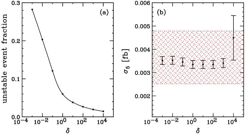
Figure 7: Dependence of the pentagon contribution to the cross section on the maximal relative numerical error, $\delta$, which is allowed for the Ward identities of the residual pentagon diagrams. The fraction $f$ of subprocess events, where a pentagon subamplitude is discarded for numerical reasons, is shown in panel (a). Panel (b) gives the pentagon contribution, $\sigma_{5}$, to the cross section. Error bars correspond to the statistical error of the Monte Carlo integration. For comparison, the statistical error on the overall cross section for a high statistics run with $\pm\,0.06\%$ accuracy is indicated by the horizontal band.

The projections of Eqs. (3.10)–(3.13) reduce the magnitude of the coefficients multiplying the pentagon loops and their overall contribution to the virtual corrections. This “true” pentagon contribution to the cross section, defined by the interference of the residual $r_{+}^{\mu_{1}}\,r_{-}^{\mu_{2}}\,\tilde{\mathcal{P}}_{\mu_{1}\mu_{2}\mu_{3}}$ type terms with the Born amplitude, is called $\sigma_{5}$ below. Minimizing it is important in view of the fact that, in the tensor-reduction procedure à la Passarino-Veltman, Gram determinants appear in the denominators of the PV coefficient functions. There are points in phase space where these determinants become small and numerical results become unstable. We have developed a strategy to interpolate over these critical points (see Ref. [22]) and, to make sure that the numerical accuracy is not spoilt, we check, numerically, that the analogs of Eqs. (3.5)–(3.7) are satisfied for the tensors $\tilde{\mathcal{P}}_{\mu_{1}\mu_{2}\mu_{3}}$. In Fig. 7 (a) we show the fraction of subprocess events, $f$ (counting pentagon corrections to the upper and the lower quark line as different subprocesses), where these Ward identities are violated by more than a fraction $\delta$. Numerical instabilities of $\delta=10\%$ or more, for example, affect about $f=13\%$ of the generated subprocess events. For subprocess events with Ward identity violations exceeding $\delta$ we discard the numerically unreliable $\widetilde{\cal M}_{V_{1}V_{2}V_{3}}$ and correct the remaining pentagon contributions by a global factor, $1/(1-f)$, in order to compensate for the loss. As demonstrated in Fig. 7 (b), this procedure leads to a constant overall pentagon contribution, $\sigma_{5}$, when varying $\delta$ between 0.001 and 1000. Numerical instabilities become large for $\delta\mathrel{\raisebox{-2.58334pt}{$\stackrel{{\scriptstyle\textstyle>}}{{\sim}}$}}10^{4}$. For our Monte Carlo runs we choose $\delta=0.1$. Since the pentagon contribution amounts to less than 0.5% of the cross section for EW $W^{+}W^{-}jj$ production with VBF cuts, the error that is induced by this approximation affects our final NLO results at an insignificant level. For comparison the shaded horizontal band shows the size of the overall cross-section uncertainty for a high-statistics run, with an overall statistical error of 0.06%.

The tensor reduction of the box-type virtual contributions is quite stable, numerically. We have checked that the corresponding Ward identities, derived in a similar way as for the pentagons, are violated at only one out of $10^{6}$ phase-space points by more than 1$\permil$.

The box- and pentagon-type virtual corrections, the finite $\widetilde{\cal M}_{V_{1}V_{2}}$ and $\widetilde{\cal M}_{V_{1}V_{2}V_{3}}$ terms in Eqs. (2.8) and (2.9), whose evaluation is cumbersome and time consuming, amount to less than one percent of the full cross section. Therefore, the statistical error of these contributions affects the accuracy of the full result only marginally and the number of Monte Carlo events for the computation of the box and pentagon corrections can be reduced substantially with respect to the Born cross section and the leading $c_{\rm virt}|{\cal M}_{B}|^{2}$ virtual contribution in Eq. (2.9): in our program, the Monte Carlo statistics is reduced by a factor 16 for the generic box contributions and by a factor 128 for the pentagon contributions after the projections of Eqs. (3.10)–(3.13). These elements, together with the efficient handling of leptonic tensors and the other speed-up “tricks” described in the previous section, yield a fast code, which allows us to perform high-statistics runs with small relative errors on the full NLO cross sections and distributions. For example, it took about five days of CPU time on a 3 GHz Pentium 4 PC to obtain an accuracy of 1$\permil$ on the distributions shown in the next section.

As discussed in detail in Ref. [8], care has to be taken in the treatment of finite-width effects in massive vector-boson propagators. In order to handle diagrams where vector bosons decay, like $W(p_{\ell}+p_{\nu})\,\mbox{$\rightarrow$}\,\ell(p_{\ell})+\nu_{\ell}(p_{\nu})$, a finite vector-boson width $\Gamma_{V}$ has to be introduced in the resonant poles of each $s$-channel vector-boson propagator. However, in the presence of single- and non-resonant graphs, like (a) and (b) in Fig. 2, this introduces violations of electroweak gauge invariance in a sub-class of diagrams, which would hold in the zero-width approximation. In the past, different methods, such as the overall factor scheme [25] and the complex-mass scheme [26], have been applied to overcome these problems. We resort to a modified version of the complex-mass scheme, which already has been used in Ref. [8]. We globally replace $m_{V}^{2}$ with $m_{V}^{2}-im_{V}\Gamma_{V}$, while keeping a real value for $\sin^{2}\theta_{W}$. This prescription has the advantage of preserving the electromagnetic Ward identity which relates the tree-level triple gauge-boson vertex and the inverse $W$ propagator [27]. It thereby avoids large contributions from gauge-invariance-violating terms.

Throughout the calculation, fermion masses are set to zero, because observation of either leptons or (light) quarks in a hadron-collider environment requires large transverse momenta and hence sizable scattering angles and relativistic energies. For consistency, external $b$- and $t$-quark contributions are excluded.

We have used a diagonal form (equal to the identity matrix) for the Cabibbo-Kobayashi-Maskawa matrix, $V_{\rm CKM}$. This approximation is not a limitation of our calculation. As long as no final-state quark flavor is tagged (no $c$ tagging is done, for example), the sum over all flavors, using the exact $V_{\rm CKM}$, is equivalent to our results, due to the unitarity of the $V_{\rm CKM}$ matrix.

The VBF cuts, discussed in Sec. 4, force the LO differential cross section for $W^{+}W^{-}jj$ to be finite, since they require two well-separated jets of finite transverse momentum. For the NLO contributions, initial-state singularities, due to collinear $q\,\mbox{$\rightarrow$}\,qg$ and $g\,\mbox{$\rightarrow$}\,q\bar{q}$ splitting, are factorized into the respective quark and gluon distribution functions of the proton. An additional divergence is encountered in those real-emission diagrams, where a $t$-channel photon of low virtuality is exchanged, thereby giving rise to a collinear $q\mbox{$\rightarrow$}q\gamma$ singularity. We avoid it by imposing a cut on the virtuality of the photon, $Q_{\gamma,\mathrm{min}}^{2}=4$ GeV². Events that do not pass this cut are considered to be part of the QCD corrections to the $p\gamma\,\mbox{$\rightarrow$}\,W^{+}W^{-}jj$ cross section, that we do not calculate here.

For the computation of cross sections and distributions presented in the following section, we have adopted the CTEQ6M parton distributions with $\alpha_{s}(m_{Z})=0.118$ at NLO, and the CTEQ6L1 set for the LO calculation [28]. The CTEQ6 parton distributions include $b$ quarks as active flavors. However, since in our calculation all fermion masses are neglected, we have disregarded external $b$- and $t$-quark contributions throughout.

We have chosen $M_{Z}=91.188$ GeV, $M_{W}=80.423$ GeV and $G_{F}=1.166\times 10^{-5}/$GeV² as electroweak input parameters. The other parameters, $\alpha_{\mathrm{QED}}=1/132.54$ and $\sin^{2}\theta_{W}=0.22217$, are computed thereof via LO electroweak relations. Final-state partons are recombined into jets according to the $k_{T}$ algorithm [29], as described in Ref. [30], with resolution parameter $D=0.8$.

4 Results for the LHC

The parton-level Monte Carlo program described in the previous section has been used to determine the size of the NLO QCD corrections to the EW $W^{+}W^{-}jj$ cross sections at the LHC. Using the $k_{T}$ algorithm, we calculate the partonic cross sections for events with at least two hard jets, which are required to have

$$p_{Tj}\geq 20~{}{\rm GeV}\,,\qquad\qquad|y_{j}|\leq 4.5\,.$$ (4.1)

Here $y_{j}$ denotes the rapidity of the (massive) jet momentum which is reconstructed as the four-vector sum of massless partons of pseudorapidity $|\eta|<5$. The two reconstructed jets of highest transverse momentum are called “tagging jets”. At LO, they are identified with the final-state quarks which are characteristic for vector-boson fusion processes.

We consider the specific leptonic final state $e^{+}\nu_{e}\,\mu^{-}\bar{\nu}_{\mu}$. One obtains the cross sections for the phenomenologically more interesting final state containing any combination of electrons or muons ($e^{+}e^{-}\nu\bar{\nu}$, $\mu^{+}\mu^{-}\nu\bar{\nu}$, $e^{\pm}\mu^{\mp}\nu\bar{\nu}$, but neglecting identical lepton interference and $ZZ$ final states) by multiplying our cross sections by a factor of 4. In order to ensure that the charged leptons are well observable, we impose the lepton cuts

$$p_{T\ell}\geq 20~{}{\rm GeV}\,,\qquad|\eta_{\ell}|\leq 2.5\,,\qquad\triangle R_{j\ell}\geq 0.4\,,$$ (4.2)

where $\triangle R_{j\ell}$ denotes the jet-lepton separation in the rapidity-azimuthal angle plane. In addition, the charged leptons are required to fall between the rapidities of the two tagging jets

$$y_{j,min}<\eta_{\ell}<y_{j,max}\,.$$ (4.3)

Backgrounds to VBF are significantly suppressed by requiring a large rapidity separation of the two tagging jets. We here impose the cut

$$\Delta y_{jj}=|y_{j_{1}}-y_{j_{2}}|>4\;.$$ (4.4)

Furthermore, we require the two tagging jets to reside in opposite detector hemispheres,

$$y_{j_{1}}\times y_{j_{2}}<0\,,$$ (4.5)

with an invariant mass

$$M_{jj}>600~{}{\rm GeV}\;.$$ (4.6)

The resulting total cross section receives two major contributions, arising from the Higgs resonance, via $H\mbox{$\rightarrow$}WW$ decays, and from the $WW$ continuum, which effectively starts at the $W$-pair threshold. Already for Higgs boson masses as low as 120 GeV, the resonance contribution is quite noticeable and, because of the strong dependence on $m_{H}$ of the $H\mbox{$\rightarrow$}WW$ branching ratio, this resonance contribution is strongly dependent on the Higgs mass. When trying to show results for the $WW$ continuum only, we therefore impose the additional requirement

$$m_{WW}=\sqrt{(p_{e}+p_{\mu}+p_{\nu_{e}}+p_{\nu_{\mu}})^{2}}\,>\,m_{H}+10\;{\rm GeV}\;,$$ (4.7)

i.e. the four-lepton invariant mass must be above the Higgs resonance. The resulting cross section is representative of the continuum above any light Higgs boson resonance ($m_{H}$ below the $W$-pair threshold).

The scale dependence of the total continuum cross section, for a Higgs boson mass of $m_{H}=120$ GeV, is shown in Fig. 8.

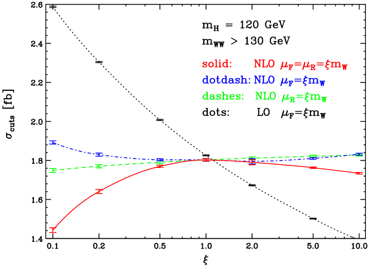
Figure 8: Scale dependence of the total $jj\,e^{+}\nu_{e}\,\mu^{-}\bar{\nu}_{\mu}$ cross section at leading and next-to-leading order within the cuts of Eqs. (4.1)–(4.7) for $pp$ collisions at the LHC. The contribution from the Higgs resonance (taken as $m_{H}=120$ GeV) is excluded. The factorization scale $\mu_{F}$ and/or the renormalization scale $\mu_{R}$ are taken as multiples of the $W$ mass, $\xi\,m_{W}$, and $\xi$ is varied in the range $0.1<\xi<10$. The NLO curves are for $\mu_{F}=\mu_{R}=\xi m_{W}$ (solid red line), $\mu_{F}=m_{W}$ and $\mu_{R}=\xi\,m_{W}$ (dashed green line) and $\mu_{R}=m_{W}$ and $\mu_{F}$ variable (dot-dashed blue line). The dotted black curve shows the dependence of the LO cross section on the factorization scale. At this order, there is no dependence on $\alpha_{s}(\mu_{R})$.

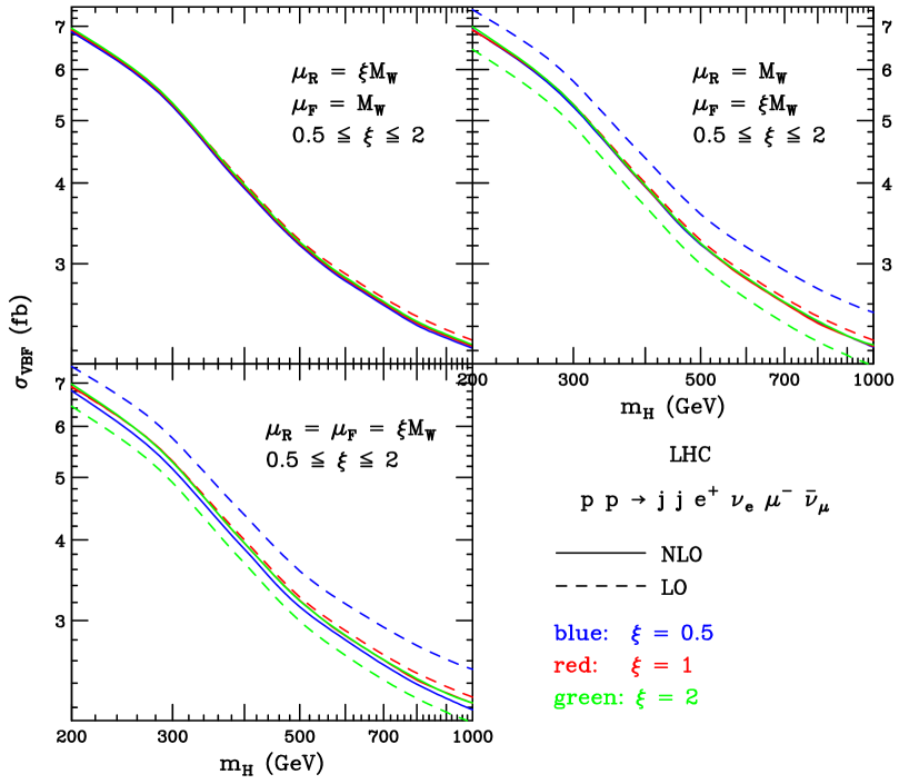
Figure 9: Higgs mass dependence of the total $pp\,\mbox{$\rightarrow$}\,jj\,e^{+}\nu_{e}\,\mu^{-}\bar{\nu}_{\mu}$ cross section at LO and NLO within the cuts of Eqs. (4.1)–(4.6). Results are shown for renormalization and factorization scales $\mu=0.5\;m_{W}$, $m_{W}$ and $2\,m_{W}$.

This figure shows the scale dependence of the LO and NLO cross sections, for renormalization and factorization scales, $\mu_{R}$ and $\mu_{F}$, which are tied to the $W$ mass

$$\mu_{R}=\xi_{R}\,m_{W}\;,\qquad\qquad\mu_{F}=\xi_{F}\,m_{W}\;.$$ (4.8)

The LO cross section only depends on the factorization scale. At NLO we show three cases: (a) $\xi_{F}=\xi_{R}=\xi$ (solid red line); (b) variation of the factorization scale only, $\xi_{F}=\xi$, $\xi_{R}=1$ (dot-dashed blue line); and (c) variation of the renormalization scale only $\xi_{R}=\xi$, $\xi_{F}=1$ (dashed green line). The NLO cross sections are quite insensitive to scale variations: allowing a factor 2 variation in either directions, i.e. considering the range $0.5<\xi<2$, the NLO cross section changes by less than 2% in all cases. Compared to this small variation, the factorization scale dependence of the LO cross section is quite sizable, amounting to a $\pm 10\%$ shift for $0.5<\xi<2$. Note that for $\mu_{F}=m_{W}$ the LO cross section is only very slightly larger than the more stable NLO result, yielding a $K$ factor  $K=\sigma_{NLO}/\sigma_{LO}=0.98$, i.e. $\mu_{F}=m_{W}$ is an excellent choice for a LO estimate of the total continuum cross section.

Also for larger Higgs boson masses, $m_{H}\mathrel{\raisebox{-2.58334pt}{$\stackrel{{\scriptstyle\textstyle>}}{{\sim}}$}}2m_{W}$, the reduction of the scale dependence at NLO is comparable to the light Higgs case. However, since the resonance contribution can no longer be trivially separated from the $WW$ continuum, we now show, in Fig. 9, the total cross section within the cuts of Eqs. (4.1)–(4.6) as a function of $m_{H}$ and for different scale choices, $\mu=\xi m_{W}$ with $\xi=0.5,\;1$ and 2. At NLO, the scale dependence is hardly visible while at LO one again finds a sizable factorization scale dependence.

The small scale dependence which is observed for the total cross section at NLO is also found for infrared-safe distributions. Typically, scale variations between $0.5\,m_{W}$ and $2\,m_{W}$ change distributions by about 2%, with somewhat larger variations, up to 6%, sometimes occurring in the tails of the distributions shown below.

The $K$ factor close to unity, which was found for the total cross section, no longer persists for distributions. We demonstrate this effect by showing a few experimentally relevant distributions together with the dynamic $K$ factor which is defined as

$$K(x)=\frac{d\sigma_{NLO}/dx}{d\sigma_{LO}/dx}\;.$$ (4.9)

In the following the Higgs boson mass is taken as $m_{H}=120$ GeV and we show cross sections for the continuum above $m_{WW}=130$ GeV and within the cuts of Eqs. (4.1)–(4.7). All panels are for the scale choice $\mu_{F}=\mu_{R}=m_{W}$.

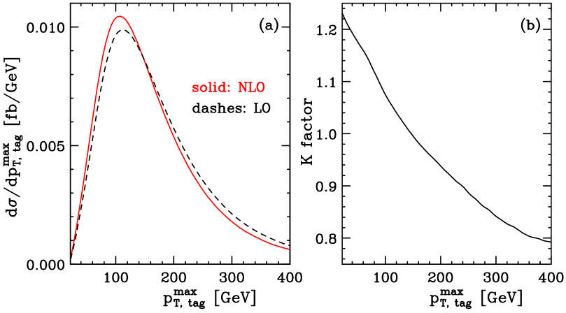
Figure 10: Transverse-momentum distribution of the highest-$p_{T}$ tagging jet in EW $W^{+}W^{-}jj$ production at the LHC. In panel (a) the NLO result (solid red line) and the LO curve (dashed black line) are shown. Their ratio, the $K$ factor  as defined in Eq. (4.9), is shown in panel (b).

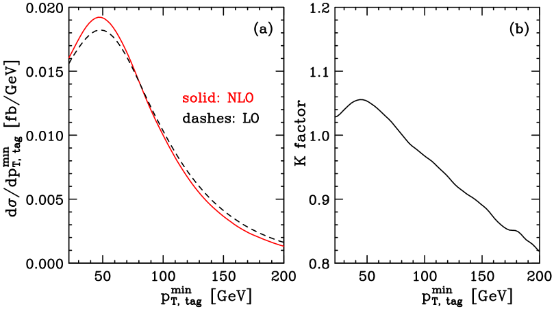
Figure 11: Same as Fig. 10 but for the smaller of the two tagging-jet transverse momenta.

A fairly strong shape change in going from LO to NLO is found for the tagging-jet transverse-momentum distributions. This is shown in Figs. 10 and 11 where the larger and the smaller of the two tagging-jet transverse momenta are shown at LO (dashed black curves) and at NLO QCD (solid red lines), together with their ratio, the $K$ factor  of Eq. (4.9). In particular the former, $d\sigma/dp_{T,{\rm tag}}^{{\rm max}}$, shows a clear shift to smaller transverse momenta at NLO, which corresponds to a $K$ factor  varying between 1.2 and 0.8 as $p_{T,{\rm tag}}^{{\rm max}}$ increases from 20 GeV to 400 GeV. The effect for $d\sigma/dp_{T,{\rm tag}}^{\rm{min}}$, in Fig. 11, is slightly smaller, but still pronounced. The change in the jet transverse-momentum distribution also feeds into the shape of the lepton transverse-momentum distributions. In Fig. 12 we depict the transverse momentum for the hardest of the two charged leptons. Again small transverse momenta are enhanced at NLO, leading to a $K$ factor between 1.04 and 0.84.

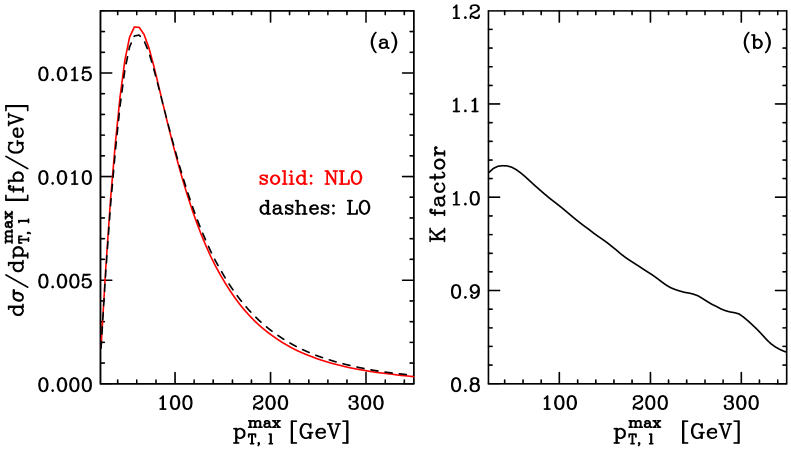
Figure 12: Transverse-momentum distributions of the hardest final-state lepton in EW $W^{+}W^{-}jj$ production at the LHC. In panel (a) the NLO result (solid red line) and the LO curve (dashed black line) are shown. Their ratio, the $K$ factor  as defined in Eq. (4.9), is shown in panel (b).

In contrast to the transverse momentum distributions, angular distributions of the leptons are hardly affected by the NLO corrections. As an example, we show the azimuthal angle between the two charged leptons in Fig. 13. The $K$ factor  is almost constant and equal to $0.98$. The typically large angle between the charged leptons is important for the reduction of $W^{+}W^{-}jj$ continuum events in the search for $H\mbox{$\rightarrow$}WW\mbox{$\rightarrow$}l^{+}l^{-}p\hskip-5.03125pt\hbox to5.03125pt{\hss$/$\hss}_{T}$ decays [4].

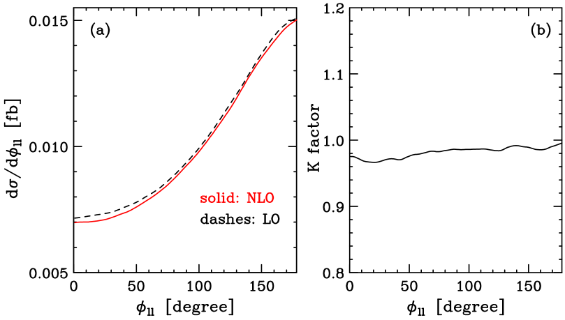
Figure 13: Azimuthal angle separation between the two charged leptons for continuum $jje^{+}\nu_{e}\,\mu^{-}\bar{\nu}_{\mu}$ events at the LHC. Curves are as in Fig. 10.

Another distribution which is important for the Higgs search at the LHC is the transverse mass of the $l^{+}l^{-}\nu\bar{\nu}$ system, which is defined as [4]

$$M_{T}^{WW}=\sqrt{({E\hskip-7.95831pt\hbox to7.95831pt{\hss$/$\hss}_{T}}+E_{T,ll})^{2}-({\bf p}_{T,ll}+{\bf p\hskip-5.55557pt\hbox to5.55557pt{\hss$/$\hss}}_{T})^{2}}\,,$$ (4.10)

where the transverse energies are given by

$$E_{T,ll} = \sqrt{{\bf p}_{T,ll}^{2}+m_{ll}^{2}}\,,$$

$$E\hskip-6.80557pt\hbox to6.80557pt{\hss/\hss}_{T} = \sqrt{{\bf p\hskip-5.55557pt\hbox to5.55557pt{\hss$/$\hss}}_{T}^{2}+m_{\nu\nu}^{2}}\approx\sqrt{{\bf p\hskip-5.55557pt\hbox to5.55557pt{\hss$/$\hss}}_{T}^{2}+m_{ll}^{2}}\,.$$ (4.11)

While the invariant mass of the $W^{+}W^{-}$ pair cannot be reconstructed, due to the presence of neutrinos, $M_{T}^{WW}$ is fully accessible. The effect of NLO QCD corrections on $M_{T}^{WW}$ is again modest, as can be seen in Fig. 14.

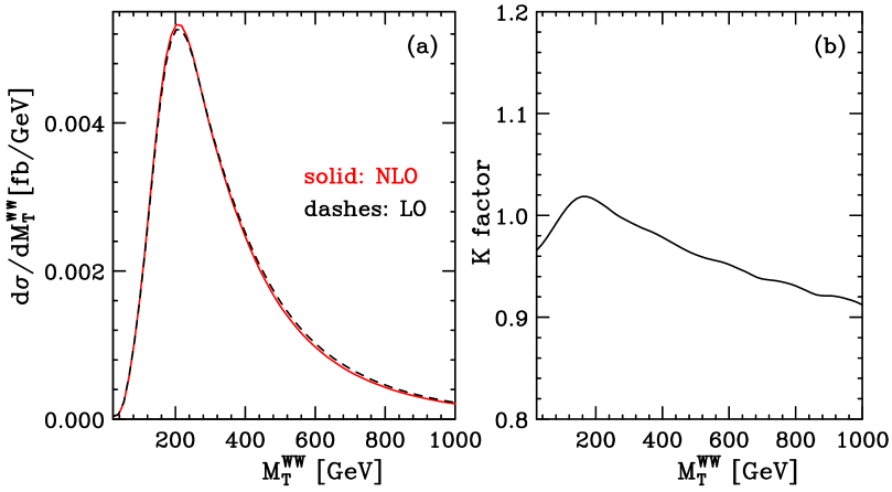
Figure 14: Transverse mass distribution for the $e^{+}\nu_{e}\,\mu^{-}\bar{\nu}_{\mu}$ system in $W^{+}W^{-}jj$ events at the LHC. Curves are as in Fig. 10. The definition of $M_{T}^{WW}$ is given in Eq. (4.10).

5 Conclusions

Vector-boson fusion at the LHC represents a class of electroweak processes which are under excellent control perturbatively. This has been known for some time for the most interesting process in this class: Higgs boson production via VBF has a modest $K$ factor of about 1.05 for the inclusive production cross section [31] and this result also holds when applying realistic acceptance cuts [7]. Similar results were also found for $Wjj$ and $Zjj$ production via VBF [8].

In the present paper, we have extended these calculations to the electroweak process $pp\,\mbox{$\rightarrow$}\,e^{+}\nu_{e}\,\mu^{-}\bar{\nu}_{\mu}\,jj$ at NLO in QCD, when the final-state particles are in a kinematic configuration typical of VBF events. This corresponds to leptonic final states in the vector-boson scattering processes $VV\mbox{$\rightarrow$}W^{+}W^{-}$ ($V$ is a $\gamma$ or a $Z$) and $W^{+}W^{-}\mbox{$\rightarrow$}W^{+}W^{-}$, but with full NLO QCD simulation of the associated tagging jets. The calculation has been implemented in the form of a fully-flexible parton level Monte Carlo program and, thus, allows to implement completely general experimental cuts. The size of the QCD corrections is similar to those found for $Hjj$ and $Vjj$ production in VBF, and corresponds to a shift of a few percent in typical integrated cross sections expected for VBF cuts. Some distributions, however, are affected somewhat more strongly, with dynamical $K$ factors ranging between 0.8 and 1.2, in particular for transverse-momentum distributions. At least as important is the stability of the NLO result: the residual scale dependence is at the 2% level for cross sections integrated within VBF cuts.

The numerical code is quite fast, reaching permille level statistics on distributions within 5 days of running on a standard 3 GHz PC. A $1\permil$ error on integrated cross sections is reached in about 1 day. This high speed has been obtained by avoiding the recalculation of recurring subamplitudes in different sub-processes contributing at a given phase-space point. A key ingredient is a modular structure of the numerical amplitude calculation which separates the weak-boson scattering sub-amplitudes into leptonic tensors, which can be changed without altering the validity of the QCD corrections. Such changes could reflect the inclusion of anomalous three- or four-vector-boson couplings or of any other new physics in weak-boson scattering. We leave such generalizations for the future.

References

- [1] ATLAS Collaboration, ATLAS TDR, Report No. CERN/LHCC/99-15 (1999); E. Richter-Was and M. Sapinski, Acta Phys. Pol. B 30, 1001 (1999); B. P. Kersevan and E. Richter-Was, Eur. Phys. J. C 25, 379 (2002) [arXiv:hep-ph/0203148].
- [2] G. L. Bayatian et al., CMS Technical Proposal, Report No. CERN/LHCC/94-38x (1994); R. Kinnunen and D. Denegri, CMS Note No. 1997/057; R. Kinnunen and A. Nikitenko, Report No. CMS TN/97-106; R. Kinnunen and D. Denegri, [arXiv:hep-ph/9907291]; V. Drollinger, T. Müller and D. Denegri, [arXiv:hep-ph/0111312].
- [3] D. Zeppenfeld, R. Kinnunen, A. Nikitenko and E. Richter-Was, Phys. Rev. D 62, 013009 (2000) [arXiv:hep-ph/0002036]; D. Zeppenfeld, in Proc. of the APS/DPF/DPB Summer Study on the Future of Particle Physics, Snowmass, 2001 edited by N. Graf, eConf C010630, p. 123 (2001) [arXiv:hep-ph/0203123]; A. Belyaev and L. Reina, JHEP 0208, 041 (2002) [arXiv:hep-ph/0205270].
- [4] D. Rainwater and D. Zeppenfeld, Phys. Rev. D 60, 113004 (1999) [Erratum-ibid. D 61, 099901 (2000)] [arXiv:hep-ph/9906218]; N. Kauer, T. Plehn, D. Rainwater and D. Zeppenfeld, Phys. Lett. B 503, 113 (2001) [arXiv:hep-ph/0012351].
- [5] J. Bagger et al., Phys. Rev. D 52 3878 (1995) [arXiv:hep-ph/9504426].
- [6] For a recent review see M. S. Chanowitz, Czech. J. Phys. 55, B45 (2005) [arXiv:hep-ph/0412203] and references therein.
- [7] T. Figy, C. Oleari and D. Zeppenfeld, Phys. Rev. D 68, 073005 (2003) [arXiv:hep-ph/0306109].
- [8] C. Oleari and D. Zeppenfeld, Phys. Rev. D 69, 093004 (2004) [arXiv:hep-ph/0310156].
- [9] R. N. Cahn and S. Dawson, Phys. Lett. B 136, 196 (1984) [Erratum-ibid. B 138, 464 (1984)]; S. Dawson, Nucl. Phys. B249, 42 (1985); M. J. Duncan, G. L. Kane and W. W. Repko, Nucl. Phys. B272, 517 (1986); J. M. Butterworth, B. E. Cox and J. R. Forshaw, Phys. Rev. D 65, 096014 (2002) [arXiv:hep-ph/0201098].
- [10] R. N. Cahn, S. D. Ellis, R. Kleiss and W. J. Stirling, Phys. Rev. D 35, 1626 (1987); R. Kleiss and W. J. Stirling, Phys. Lett. B 200, 193 (1988); V. Barger, T. Han and R. J. N. Phillips, Phys. Rev. D 37, 2005 (1988).
- [11] J. F. Gunion, J. Kalinowski and A. Tofighi-Niaki, Phys. Rev. Lett. 57, 2351 (1986); D. A. Dicus and R. Vega, Phys. Rev. Lett. 57, 1110 (1986); Phys. Rev. D 37, 2474 (1988).
- [12] U. Baur and E. W. N. Glover, Phys. Lett. B 252, 683 (1990).
- [13] V. D. Barger, K. M. Cheung, T. Han and D. Zeppenfeld, Phys. Rev. D 44 2701 (1991) [Erratum-ibid. D 48 5444 (1993)].
- [14] A. Duff and D. Zeppenfeld, Phys. Rev. D 50 3204 (1994) [arXiv:hep-ph/9312357].
- [15] E. Accomando, A. Ballestrero, S. Bolognesi, E. Maina and C. Mariotti, arXiv:hep-ph/0512219; E. Accomando, A. Ballestrero, A. Belhouari and E. Maina, arXiv:hep-ph/0603167.
- [16] K. Hagiwara and D. Zeppenfeld, Nucl. Phys. B274, 1 (1986); K. Hagiwara and D. Zeppenfeld, Nucl. Phys. B313, 560 (1989).
- [17] T. Stelzer and W. F. Long, Comput. Phys. Commun. 81, 357 (1994) [arXiv:hep-ph/9401258]; F. Maltoni and T. Stelzer, JHEP 0302, 027 (2003) [arXiv:hep-ph/0208156].
- [18] F. Boudjema et al., arXiv:hep-ph/9601224.
- [19] S. Catani and M. H. Seymour, Nucl. Phys. B485, 291 (1997) [Erratum-ibid. B510, 503 (1997)] [arXiv:hep-ph/9605323].
- [20] Warren Siegel, Phys. Lett. B 84, 193 (1979); Warren Siegel, Phys. Lett. B 94, 37 (1980).
- [21] G. Passarino and M. J. Veltman, Nucl. Phys. B160, 151 (1979).
- [22] C. Oleari and D. Zeppenfeld. In preparation.
- [23] Z. Bern, L. Dixon and D. Kosower, Phys. Lett. B302, 299 (1993), Erratum-ibid. B318, 649 (1993) [hep-ph/9212308]; Z. Bern, L. Dixon and D. Kosower, Nucl. Phys. B412, 751 (1994) [hep-ph/9306240].
- [24] G. Duplancic and B. Nizic, Eur. Phys. J. C 20, 357 (2001) [arXiv:hep-ph/0006249].
- [25] U. Baur, J. A. Vermaseren and D. Zeppenfeld, Nucl. Phys. B375, 3 (1992).
- [26] A. Denner, S. Dittmaier, M. Roth and D. Wackeroth, Nucl. Phys. B560, 33 (1999) [arXiv:hep-ph/9904472].
- [27] See, e.g., G. Lopez Castro, J.L.M. Lucio and J. Pestieau, Mod. Phys. Lett. A6, 3679 (1991); M. Nowakowski and A. Pilaftsis, Z. Phys. C60, 121 (1993); U. Baur and D. Zeppenfeld, Phys. Rev. Lett. 75, 1002 (1995) [arXiv:hep-ph/9503344], and references therein.
- [28] J. Pumplin, D. R. Stump, J. Huston, H. L. Lai, P. Nadolsky and W. K. Tung, JHEP 0207, 012 (2002) [arXiv:hep-ph/0201195].
- [29] S. Catani, Yu. L. Dokshitzer and B. R. Webber, Phys. Lett. B 285 291 (1992); S. Catani, Yu. L. Dokshitzer, M. H. Seymour and B. R. Webber, Nucl. Phys. B406 187 (1993); S. D. Ellis and D. E. Soper, Phys. Rev. D 48 3160 (1993).
- [30] G. C. Blazey et al., arXiv:hep-ex/0005012.
- [31] T. Han, G. Valencia and S. Willenbrock, Phys. Rev. Lett. 69, 3274 (1992) [arXiv:hep-ph/9206246].