Constrained invariant mass distributions in cascade decays. The shape of the “$m_{qll}$-threshold” and similar distributions.

Abstract

Considering the cascade decay $D\rightarrow cC\rightarrow cbB\rightarrow cbaA$ in which $D,C,B,A$ are massive particles and $c,b,a$ are massless particles, we determine for the shape of the distribution of the invariant mass of the three massless particles $m_{abc}$ for the sub-set of decays in which the invariant mass $m_{ab}$ of the last two particles in the chain is (optionally) constrained to lie inside an arbitrary interval, $m_{ab}\in[m_{ab}^{\text{cut min}},m_{ab}^{\text{cut max}}]$. An example of an experimentally important distribution of this kind is the “$m_{qll}$ threshold” – which is the distribution of the combined invariant mass of the visible standard model particles radiated from the hypothesised decay of a squark to the lightest neutralino via successive two body decay,: ${\tilde{q}}\rightarrow q{\tilde{\chi}_{2}^{0}}\rightarrow ql{\tilde{l}}\rightarrow qll{\tilde{\chi}_{1}^{0}}$, in which the experimenter requires additionally that $m_{ll}$ be greater than ${m_{ll}^{max}}/\sqrt{2}$. The location of the “foot” of this distribution is often used to constrain sparticle mass scales. The new results presented here permit the location of this foot to be better understood as the shape of the distribution is derived. The effects of varying the position of the $m_{ll}$ cut(s) may now be seen more easily.

1 Introduction

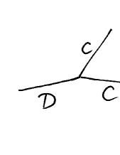
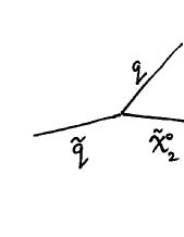
Figure 1: The decay chain under study. Part (a) shows the chain in “generic” form with the massive particles on the “backbone” labelled with capital letters, and the massless visible particles labelled in lower case. Part (b) shows a commonly hypothesised squark decay chain open in many supersymmetric models. This particular chain is the example most frequently used to motivate the study of the “generic” chain in part (a).

We consider the cascade decay $D\rightarrow cC\rightarrow cbB\rightarrow cbaA$ shown in figure 1 in which $D,C,B,A$ are massive particles and $c,b,a$ are treated as massless particles.

In the context of the Large Hadron Collider (LHC), the most studied example of such a decay chain is the hypothesised decay of a squark to the lightest neutralino via three successive two body decays: ${\tilde{q}}\rightarrow q{\tilde{\chi}_{2}^{0}}\rightarrow ql{\tilde{l}}\rightarrow qll{\tilde{\chi}_{1}^{0}}$. The decay chain is relevant to more than just supersymmetric decays, however. For example it may appear in models with extra dimensions, in which the particles would be Kaluza-Klein excitations.

It has been frequently suggested [1, 2, 3, 4, 5] that one of the main ways we might hope to measure or constrain the masses of new particles produced at the LHC will be through the study of kinematic endpoints of invariant masses constructed from the visible products of decay chains like those in figure 1.

Given the observed four-momenta $a^{\mu}$, $b^{\mu}$ and $c^{\mu}$ it is in principle possible to construct three non-trivial linearly-independent Lorentz-invariant quantities, namely $m_{ab}^{2}=(a^{\mu}+b^{\mu})^{2}$, $m_{bc}^{2}=(b^{\mu}+c^{\mu})^{2}$ and $m_{ac}^{2}=(a^{\mu}+c^{\mu})^{2}$. A fourth quantity $m_{abc}^{2}=(a^{\mu}+b^{\mu}+c^{\mu})^{2}$ is related to the first three via $m_{abc}^{2}=m_{ab}^{2}+m_{bc}^{2}+m_{ac}^{2}$.

In many models in which this decay chain is present, however, it is not possible to tell two of the particles apart (typically $a$ and $b$). For example, in the supersymmetric decay chain ${\tilde{q}}\rightarrow q{\tilde{\chi}_{2}^{0}}\rightarrow ql{\tilde{l}}\rightarrow qll{\tilde{\chi}_{1}^{0}}$ the particles $a$ and $b$ form a lepton-antilepton pair, and it may be impossible to say which observed lepton was the “$a$” and which was the “$b$”. In such models, the three independent variables are instead ${m_{ab}^{2}}$, ${({m_{ql}^{\text{high}}})^{2}}=\max{[{m_{ac}^{2}},{m_{bc}^{2}}]}$ and ${({m_{ql}^{\text{low}}})^{2}}=\min{[{m_{ac}^{2}},{m_{bc}^{2}}]}$. We see that the experimentally unidentifiable ${m_{ac}^{2}}$ and ${m_{bc}^{2}}$ have been replaced by experimentally observable ${({m_{ql}^{\text{high}}})^{2}}$ and ${({m_{ql}^{\text{low}}})^{2}}$. Note that as before, $m_{abc}^{2}=m_{ab}^{2}+{({m_{ql}^{\text{high}}})^{2}}+{({m_{ql}^{\text{low}}})^{2}}$.

Although there are only three independent variables that categorise a given decay, by looking at more than one event of the given decay type it is often possible to construct more than three independent constraints on the masses of the particles involved. This has been done most frequently by constructing new variables which are arbitrary functions of the three independent variables, and then looking for the kinematic endpoints of the distributions of these variables over a large number of events.

In principle the shape of any one of these distributions contains more information than the position of the associated kinematic endpoint. Nonetheless, in previous years there has been a tendency to concentrate mainly on constraints coming from kinematic endpoints because interpreting these constraints does not require a detailed understanding of the way detector acceptance and reconstruction efficiency may vary across any of these distributions. Such detector effects may not be known with great confidence until a number of years after LHC turn-on.

Recently, however, there has been a resurgence of interest in understanding the shapes of these kinematic distributions [7, 8] not least because an understanding of the shapes of these distributions is a pre-requisite for being able to fit the positions of the kinematic endpoints, even if one chooses to ignore all the information contained in the rest of the shape. In particular [8] has recently calculated the shapes of the distributions of the $m_{ab}$, ${m_{ql}^{\text{high}}}$, ${m_{ql}^{\text{low}}}$ and ${m_{abc}}$ distributions. One distribution whose shape was not calculated in [8] or elsewhere, however, was the shape of the ${m_{abc}^{\text{thresh}}(x)}$ distribution.

Specifically the ${m_{abc}^{\text{thresh}}(x)}$ distribution is a constrained form of the ${m_{abc}}$ distribution in which the only events which are considered are those for which the value of $m_{ab}$ happens to exceed a cut $x={m_{ab}^{\text{cut min}}}$ which is most frequently chosen to be $1/\sqrt{2}$ times the maximum value which ${m_{ab}}$ can take. The lower kinematic endpoint is the one whose position is most sensitive to the additional constraint (although the position of the upper endpoint can also be modified), and hence it is called a “threshold” rather than a “maximum”. The ${m_{abc}^{\text{thresh}}(x)}$ distribution is used because the position of the threshold, as a function of the masses of the particles involved, is more non-linear than the locations of other endpoints. This means that the position of the threshold can sometimes provide a handle on the absolute mass scale of the particles involved. Without a constraint from the endpoint of the ${m_{abc}^{\text{thresh}}(x)}$ distribution, the other edges usually only succeed in constraining mass differences.

Though important, the shape of threshold of the ${m_{abc}^{\text{thresh}}(x)}$ distribution has been poorly studied in the past. Poor understanding of the shape of this edge has frequently resulted in the location of this endpoint being assigned a large systematic error (see for example [1, 2, 3, 4, 5]). Even allowing for a larger systematic error on the edge measurement, it often seems to be the case that the displacement of this edge from its “nominal” value is greater than a naive interpretation of the edge as a straight line would lead one to expect.

We redress the historical imbalance in this note, by determining the shape of the ${m_{abc}^{\text{thresh}}(x)}$ distribution in the spinless approximation, which is valid for supersymmetry at the LHC. We do this for arbitrary values of $x={m_{ab}^{\text{cut min}}}$, the imposed lower-bound requirement on ${m_{ab}}$. Given the form of the method, it turns out to be no extra effort to allow also an arbitrary upper-bound requirement ${m_{ab}^{\text{cut max}}}$ on ${m_{ab}}$, should one wish to exploit the information contained in the changes to the upper part of the distribution caused by varying this quantity.

1.1 Existing results from earlier work

First we note some existing results which we will make use of in later sections. [2] (and many of the references in the Supersymmetry Chapter therein) told us that:

$${(m_{ab}^{\text{max}})^{2}}=\frac{({m_{C}^{2}}-{m_{B}^{2}})({m_{B}^{2}}-{m_{A}^{2}})}{{m_{B}^{2}}},$$ (1)

Also [3, 4] told us that

$${(m_{abc}^{\text{max}})^{2}}=\begin{cases}({m_{D}^{2}}-{m_{C}^{2}})({m_{C}^{2}}-{m_{A}^{2}})/{m_{C}^{2}}&\text{iff ${m_{C}^{2}}<{m_{A}}{m_{D}}$},\\ ({m_{D}^{2}}-{m_{B}^{2}})({m_{B}^{2}}-{m_{A}^{2}})/{m_{B}^{2}}&\text{iff ${m_{A}}{m_{D}}<{m_{B}^{2}}$},\\ ({m_{D}^{2}}{m_{B}^{2}}-{m_{C}^{2}}{m_{A}^{2}})({m_{C}^{2}}-{m_{B}^{2}})/({m_{C}^{2}}{m_{B}^{2}})&\text{iff ${m_{B}^{2}}{m_{D}}<{m_{A}}{m_{C}^{2}}$},\\ ({m_{D}}-{m_{A}})^{2}&\text{otherwise.}\end{cases}$$ (2)

It was also shown in [3] and more recently in [9] that

$${(m_{abc}^{\text{thresh}}(x))^{2}}=x^{2}+2E^{(C)}_{c}(E_{ab}^{(C)}(x)-p_{ab}^{(C)}(x))$$ (3)

where

$$E_{c}^{(C)} = \frac{{m_{D}^{2}}-{m_{C}^{2}}}{2{m_{C}}},$$ (4)

$$(p_{ab}^{(C)}(x))^{2} = \frac{({m_{C}^{2}}+{m_{A}^{2}}-x^{2})^{2}-4{m_{C}^{2}}{m_{A}^{2}}}{4{m_{C}^{2}}}\qquad\quad\text{and}$$ (5)

$$E_{ab}^{(C)(x)} = \sqrt{x^{2}+(p_{ab}^{(C)}(x))^{2}}$$ (6)

$$= \frac{x^{2}+({m_{C}^{2}}-{m_{A}^{2}})}{2{m_{C}}},$$ (7)

where $x={m_{ab}^{\text{cut min}}}$ is the smallest value of ${m_{ab}}$ which events are allowed to have if they are to become part of the “threshold distribution”.

2 Result

The main result of this paper is that:

$$\frac{1}{\Gamma_{\text{Tot}}}{\frac{d\Gamma}{d({m_{abc}^{2}})}}={P({m_{abc}^{2}})}$$ (8)

where

$${P({m_{abc}^{2}})}=\begin{cases}\left[{J(\beta)-J(\alpha)}\right]\Theta\left({\beta-\alpha}\right)/Z&\text{if ${m_{abc}^{2}}\leq({m_{D}}-{m_{A}})^{2}$}\\ 0&\text{otherwise.}\\ \end{cases}$$ (9)

In the above we have defined the function

$$J(x)=-\cosh^{-1}\left(\frac{{m_{C}^{2}}+{m_{A}^{2}}-x}{2{m_{C}}{m_{A}}}\right)$$ (10)

and defined the quantities

$$\beta = \min\left[{({m_{ab}^{\text{cut max}}})^{2}},{(m_{ab}^{+})^{2}},{(m_{ab}^{\text{max}})^{2}}\right],$$ (11)

$$\alpha = \max\left[{({m_{ab}^{\text{cut min}}})^{2}},{(m_{ab}^{-})^{2}},0\right]$$ (12)

in which

$${(m_{ab}^{\pm})^{2}}=\frac{1}{2{m_{D}^{2}}}\left[{({m_{D}^{2}}+{m_{C}^{2}}){m_{abc}^{2}}-({m_{D}^{2}}-{m_{C}^{2}})\left\{({m_{D}^{2}}-{m_{A}^{2}})\mp\sqrt{X^{4}}\right\}}\right]$$ (13)

in which

$$X^{4}=({m_{D}^{2}}+{m_{A}^{2}}-{m_{abc}^{2}})^{2}-4{m_{A}^{2}}{m_{D}^{2}}.$$ (14)

If the normalising constant $Z$ in (9) is chosen to be

$$Z=\left(\frac{{m_{D}^{2}}-{m_{C}^{2}}}{{m_{C}^{2}}}\right)\left({({m_{ab}^{\text{cut max}}})^{2}}-{({m_{ab}^{\text{cut min}}})^{2}}\right),$$ (15)

then the integral of ${P({m_{abc}^{2}})}$ over physical values of ${m_{abc}^{2}}$ is fixed at unity. This makes ${P({m_{abc}^{2}})}$ into a normalised probability distribution, suitable for use in log likelihood fits, etc. The function $\Theta(x)$ in (9) is the Heaviside Step Function, equal to 0 for $x<0$ and equal to 1 for $x>=0$. If desired, the normalised distribution in mass space (rather than mass-squared space) is easily found via

$$\frac{1}{\Gamma_{\text{Tot}}}{\frac{d\Gamma}{d({m_{abc}})}}=2{m_{abc}}\frac{1}{\Gamma_{\text{Tot}}}{\frac{d\Gamma}{d({m_{abc}^{2}})}}.$$ (16)

Remarks

For the “classic” $m_{qll}$-threshold of [1, 2, 3, 4, 5], the following choices are made:

$${({m_{ab}^{\text{cut max}}})^{2}} = {(m_{ab}^{\text{max}})^{2}},$$ (17)

$${({m_{ab}^{\text{cut min}}})^{2}} = {(m_{ab}^{\text{max}})^{2}}/2.$$ (18)

One can recover the standard “full” ${m_{abc}^{2}}$ distribution (i.e. the distribution whose upper edge provides the measurement, not the constrained threshold distribution derived from it by applying extra cuts) by setting ${({m_{ab}^{\text{cut min}}})^{2}}$ in (18) to zero.

Neither the final argument to the $\min$ in (11) nor the final argument to the $\max$ in (12) is strictly necessary. These arguments are there only to protect against accidental unphysical choices of ${({m_{ab}^{\text{cut max}}})^{2}}$ and ${({m_{ab}^{\text{cut min}}})^{2}}$, i.e. values which do not satisfy

$$0\leq{({m_{ab}^{\text{cut min}}})^{2}}\leq{({m_{ab}^{\text{cut max}}})^{2}}\leq{(m_{ab}^{\text{max}})^{2}}.$$ (19)

The normalising constant $Z$ in (15) has not been similarly protected, so care should be taken to ensure that (19) is satisfied when evaluating $Z$.

If the function $J(x)$ is only evaluated when (9) demands it, $X^{4}$ will always be non-negative and its square root may safely be taken in (13).

Despite what the notation may appear to imply, either (or indeed both) of ${(m_{ab}^{+})^{2}}$ and ${(m_{ab}^{-})^{2}}$ can be negative. It is important to retain the signs of these quantities when they are used in equations (11) and (12).

In mass-squared-space (i.e. plotting ${\frac{d\Gamma}{d({m_{abc}^{2}})}}$ rather than ${\frac{d\Gamma}{d({m_{abc}})}}$) the shape of the distribution resembles a “top-hat distribution with sloping sides” as shown in figure 2. The flat upper part of the top-hat begins and ends at roots of ${({m_{ab}^{\text{cut max}}})^{2}}={(m_{ab}^{+})^{2}}$ or ${({m_{ab}^{\text{cut min}}})^{2}}={(m_{ab}^{-})^{2}}$ which are the places at which the $max$ and $min$ functions in (11) and (12) have cusps. Though not straight lines, the “flanks” of the distribution are often not strongly curved, and so in the absence of effects from resolution, detector acceptance and other cuts, and in the absence of contamination from non-pure chains the lower edge should vanish linearly. This effect is not altered significantly by the transition from mass-squared space to mass space, unless the threshold is itself very close to the origin, whereupon the edge takes on a quadratic character.

Figure 2: Cartoon of the shape of the ${m_{abc}^{2}}$ distribution defined in (9). Note the distribution is over the square of the mass, not over the mass itself.

3 Selection cuts and impurities

Event selection cuts (and other effects) modify the shape of the $m_{qll}$-threshold distribution.

We illustrate this by generating a 100 inverse femtobarn sample of general SUSY events using Herwig 6.1 [10] and pass them through a simple detector simulation [11] which crudely models the response of the ATLAS LHC experiment. Following [1, 2, 3, 4] and others, we work with the minimal SUGRA model known as “SUGRA Point 5” defined by $m_{0}=100~{}{{\rm{GeV}}}$, $m_{\frac{1}{2}}=300~{}{{\rm{GeV}}}$, $A_{0}=300~{}{{\rm{GeV}}}$, $\tan\beta=2.1$ and $\mu>0$. This model has $m_{\tilde{\chi}_{1}^{0}}=121.5~{}{{\rm{GeV}}}$, $m_{\tilde{e}_{R}}=157.2~{}{{\rm{GeV}}}$, $m_{\tilde{\chi}_{2}^{0}}=233~{}{{\rm{GeV}}}$ and has squarks of order $650-660~{}{{\rm{GeV}}}$ (although the lightest stop is much lighter at $494~{}{{\rm{GeV}}}$).

When constructing the “experimentally observed” $m_{qll}$-threshold distribution, we use exactly the procedure described in [3], which is to say in summary:

• We require ${n_{\rm leptons}}=2$, both leptons are opposite-sign same-family (OSSF) and ${p_{T}^{l_{1}}}\geq{p_{T}^{l_{2}}}\geq 10~{}{{\rm{GeV}}}$.

• We require ${n_{\rm jets}}\geq 2$ and ${p_{T}^{j_{1}}}\geq{p_{T}^{j_{2}}}\geq 150~{}{{\rm{GeV}}}$.

• We require $\hbox to0.0pt{\hbox to5.03125pt{\hfil/\hfil}\hss}p_{T}\geq 300\ {{\rm{GeV}}}$.

• We form only the larger of the two possible $m_{qll}$ combinations (one for each of $j_{1}$ and $j_{2}$) as our main interest is in preserving the quality of the lower edge, which we do not wish to obscure with wrong-combination backgrounds. This jet-choice ensures wrong-choice backgrounds fall at high rather than at low mass values.

• We repeat the above set of selection cuts but for opposite-sign different-family (OSDF) leptons. We add these events with weight -1 to the final histogram in order to subtract backgrounds from uncorrelated leptons.

The resultant “experimentally observed” $m_{qll}$-threshold distribution may be seen in figure 3(a). Figure 3(b) breaks this distribution down into the components in which the jet was correctly or incorrectly identified, and figure 3(c) shows the distribution predicted by the mass-space form of (9) using the masses $m_{\tilde{\chi}_{1}^{0}}=121.5$, $m_{\tilde{l}}=157.2$, $m_{\tilde{\chi}_{2}^{0}}=233$ and $m_{\tilde{q}}=656~{}{{\rm{GeV}}}$. The first three masses are taken directly from the model. The final mass represents the mass of a “typical” squark - an average of the masses of the twelve squarks participating in the chain.

The figure shows that there is good agreement between the analytic shape in 3(c) and the “correct combination” component of the “experimentally observed” distribution, even though the jet-selection method should introduce a slight skew to the “correct combination” component. It seems that for these masses the skew is not very noticeable. The presence of the significant “wrong combination” background, however, means that it is important not to use the analytic shape on its own.

When the $m_{qll}$-threshold analysis was first proposed [1] the analytic form of the shape was not known. This motivated the deliberately high-mass-biasing jet-choice which seeks to keep the threshold of the mass distribution clean. Now that the shape of the distribution is known, it may prove more fruitful in later studies to bin both jet combinations, and then fit the analytic shape on top of a continuum background whose shape could perhaps be estimated from the side bands.

Figure 3: Three sets of $m_{qll}$-threshold distributions for the CMSSM mSUGRA model described in the text. (a) shows what might be seen in a typical LHC experiment after the cuts described in the text. Figure (b) shows (a) broken down into the four components which contribute to it. These are (1) a narrow component coming from events in which the jet was correctly identified (solid line), (2) a broad component in which the jet was incorrectly identified (dashed line), (3) a small component representing the contribution from all SUSY sources which have nothing to do with the desired chain (dotted line), and finally (4) a small component from all SUSY sources which pass opposite-sign different-family versions of the cuts (dot-dashed line). The shape of component (4) matches the shape of (3) nicely and is added with negative weight in (a) to subtract component (3). Figure (c) shows the shape of the $m_{qll}$-threshold distribution as predicted in the text using the masses $m_{\tilde{\chi}_{1}^{0}}=121.5$, $m_{\tilde{l}}=157.2$, $m_{\tilde{\chi}_{2}^{0}}=233$ and $m_{\tilde{q}}=656~{}{{\rm{GeV}}}$.

4 Conclusions

The shape of the distribution of the total invariant mass of the light particles emitted in the decays shown in figure 1 has been calculated for the sub-set of decays which pass an additional upper and/or lower cut on the invariant mass of the last two particles emitted in the decay. This distribution is known generically as the $m_{abc}$-threshold distribution, or in its most commonly used specific example as the $m_{qll}$-threshold distribution. Even though the calculation treats all particles involved as scalars, the result is still exact in many cases, and will remain a good approximation in many others. The “classic” $m_{qll}$-threshold distribution in supersymmetry is one of the places where the spinless approximation is exact, as spin effects from $ql^{+}l^{-}$ cancel those from $ql^{-}l^{+}$. Deviations from the spinless approximation are potentially observable in UED and other non-susy models where spin effects in $q^{*}l^{+}l^{-}$ and $q^{*}l^{-}l^{+}$ do not cancel completely, although the magnitude of these deviations are likely to be small as the production excess of $q^{*}$ over ${\bar{q}}^{*}$ is itself expected to be small at the LHC over much of parameter space.

5 Acknowledgements

The author would like to thank D. T. Koch, A. R. Raklev and members of the Cambridge Supersymmetry Working Group (in particluar J. Smillie and A. J. Barr) for helpful comments and discussions.

6 Appendix

The derivation of the result (9) may be achieved using the following steps.

• Work in the rest frame of the $C$.

• In this frame the energy of the $c$ is calculable (see (4)), as is the energy of the $(a+b)$-system if it is taken to be an effective particle of known mass $m_{ab}$ (see (6)).

• The mass-squared $m_{ab}^{2}$ may easily be shown to be distributed uniformly, and the polar angle $\theta$ between the $c$ and the $(a+b)$-system in this frame will be uniform in $\cos\theta$ if either the spin of the $C$ may be neglected or if we are unable (or choose not) to distinguish contributions from different spins. This will happen at the LHC where no distinction will be drawn between $e^{+}e^{-}$ events and $e^{-}e^{+}$ events. As a result we have:

  $$\Gamma\propto\int_{I}d{(\cos\theta)}d{({m_{ab}^{2}})}.$$ (20)

• Change variables from $\cos\theta$ to ${m_{abc}^{2}}$, resulting in

  $$\Gamma\propto\int_{I}\frac{1}{2{m_{C}}p_{ab}^{(C)}}d{({m_{abc}^{2}})}d{({m_{ab}^{2}})}.$$ (21)

• The boundary of the region $I$ may be shown in $({m_{ab}^{2}},{m_{abc}^{2}})$-space to be the intersection of the interior of one half of a hyperbola with a vertical strip of constant width in ${m_{ab}^{2}}$ (starting at ${({m_{ab}^{\text{cut min}}})^{2}}$ and ending at ${({m_{ab}^{\text{cut max}}})^{2}}$).

• It is possible to write the integration limits for $I$ as upper and lower bounds on ${m_{ab}^{2}}$ (respectively $\beta$ and $\alpha$ in (11) and (12)) for given ${m_{abc}^{2}}$, allowing the order of integration to be exchanged, and the integral over ${m_{ab}^{2}}$ to be performed analytically:

  $$\Gamma \propto \int\int_{\alpha}^{\beta}\frac{1}{2{m_{C}}p_{ab}^{(C)}}d{({m_{ab}^{2}})}d{({m_{abc}^{2}})}$$ (22)

  $$= \int\left[-cosh^{-1}\left(\frac{{m_{C}^{2}}+{m_{A}^{2}}-x}{2{m_{C}}{m_{A}}}\right)\right]^{x=\beta}_{x=\alpha}d{({m_{abc}^{2}})}.$$ (23)

  from which the form of ${P({m_{abc}^{2}})}$ can be read directly.

• The value of $Z$ needed to normalise ${P({m_{abc}^{2}})}$ to unit area is found by performing the remaining integral.

References

- [1] H. Bachacou, I. Hinchliffe, F. E. Paige, Measurements of masses in SUGRA models at LHC, Phys. Rev. D62 (2000) 015009.
- [2] A. Collaboration, ATLAS detector and physics performance Technical Design Report, CERN/LHCC 99-15, 1999.
- [3] C. G. Lester, Model independant sparticle mass measurements at atlas, Ph.D. thesis, University of Cambridge, 2001, CERN-THESIS-2004-003, http://cdsweb.cern.ch/search.py?sysno=002420651CER.
- [4] B. C. Allanach, C. G. Lester, M. A. Parker, B. R. Webber, Measuring sparticle masses in non-universal string inspired models at the LHC, JHEP 09 (2000) 004.
- [5] C. G. Lester, M. A. Parker, M. J. White, Determining SUSY model parameters and masses at the LHC using cross-sections, kinematic edges and other observables, JHEP 01 (2006) 080.
- [6] A. J. Barr, Using lepton charge asymmetry to investigate the spin of supersymmetric particles at the LHC, Phys. Lett. B596 (2004) 205–212.
- [7] B. K. Gjelsten, D. J. Miller, P. Osland, Measurement of susy masses via cascade decays for SPS 1a, JHEP 12 (2004) 003.
- [8] D. J. Miller, P. Osland, A. R. Raklev, Invariant mass distributions in cascade decaysHep-ph/0510356.
- [9] R. Kitano, Y. Nomura, Supersymmetry, naturalness, and signatures at the LHC.
- [10] G. Corcella, et al., Herwig 6: An event generator for hadron emission reactions with interfering gluons (including supersymmetric processes), JHEP 01 (2001) 010.
- [11] E. Richter-Was, D. Froidevaux, L. Poggioli, ATLFAST 2.0 a fast simulation package for ATLAS, CERN (1998) 1–79 ATL-PHYS-98-131, http://cdsweb.cern.ch/search.py?recid=683751.