KIAS–P06010

ICRR-Report–524–2005–7

March 2006

Abundance of Cosmological Relics in Low–Temperature Scenarios

Manuel Drees${}^{a,b,\,}$, Hoernisa Iminniyaz${}^{a,c,\,}$, Mitsuru Kakizaki${}^{a,d,\,}$

^aPhysikalisches Institut der Universität Bonn, Nussallee 12, 53115 Bonn, Germany
^bKorea Institute of Advanced Studies, School of Physics, Seoul 130–012, South Korea
^cPhysics Dept., Univ. of Xinjiang, 830046 Urumqi, P.R. China
^dICRR, Univ. of Tokyo, Kashiwa 277-8582, Japan

1 Introduction

The production of massive, long–lived or stable relic particles $\chi$ plays a crucial role in particle cosmology [1]. The perhaps most important example is the production of Massive Weakly–Interacting Particles (WIMPs), which may constitute most of the Dark Matter in the universe [2]. Alternatively, WIMPs may only be meta–stable, and decay into even more weakly interacting particles (e.g. gravitinos or axinos) that form the Dark Matter [3]. Even if WIMP decays do not produce Dark Matter particles, the WIMP density is tightly constrained by analyses of Big Bang Nucleosynthesis (BBN)[4].

It is usually assumed that the WIMPs were in full thermal and chemical equilibrium in the radiation–dominated epoch after the period of last entropy production, which in standard cosmology means after the end of inflation. In this “standard” scenario the $\chi$ number density $n_{\chi}(T)$ drops exponentially once the temperature $T$ falls below the mass $m_{\chi}$ of the relic particles, until the freeze–out temperature $T_{F}$ is reached, where the production of $\chi$ particles from the thermal bath becomes negligible. In this case accurate semi–analytical expressions for $n_{\chi}(T\ll T_{F})$ have been derived [5, 6]; one finds that the $\chi$ relic density is essentially inversely proportional to the thermal average of the effective $\chi$ annihilation cross section into lighter particles. The case of additional late entropy production, at $T\ll T_{F}$, can also be treated analytically, by multiplying the standard result with a “dilution factor” due to the late–produced entropy [7].

For typical WIMP scenarios, $T_{F}\simeq m_{\chi}/20$. The standard treatment can work only if the maximal temperature after inflation, usually called the reheat temperature $T_{R}$, is (much) larger than $T_{F}$. The assumption $T_{R}\gg T_{F}$ is not implausible, since the scale of inflation has to be quite high, typically $\sim 10^{13}$ GeV in simple models, in order to achieve the right order of magnitude of density perturbations [8]. On the other hand, we have direct observational evidence (from BBN) only for temperatures $T\raisebox{-3.69899pt}{~{}\shortstack{$<$ \\ [-0.07cm] $\sim$}}~{}$ (few) MeV [9, 10], which is well below $T_{F}$ for most current WIMP candidates [2]. It is therefore legitimate to investigate scenarios with $T_{R}\raisebox{-3.69899pt}{~{}\shortstack{$<$ \\ [-0.07cm] $\sim$}}~{}T_{F}$ [11, 12, 13].

We should emphasize at this point that $T_{R}$ may not have been the highest temperature of the thermal plasma after inflation: given sufficiently fast thermalization, the inflaton decay products can attain a temperature $T_{\rm max}\gg T_{R}$ while the total energy density of the universe is still dominated by inflatons [1]. $\chi$ particles may therefore have been in thermal equilibrium for some range of temperatures $T>T_{R}$ [14, 9, 15, 11, 16], even if they never were in equilibrium in the radiation–dominated epoch. However, an analytical treatment of the re–heating epoch where $T>T_{R}$ was possible faces several complications not present in the radiation–dominated epoch: the entropy density was not constant, non–perturbative (and non–exponential) inflaton decays might have been important [17], and there might have been significant non–thermal sources of $\chi$ particles [18, 15, 16]. On the other hand, in supersymmetric scenarios thermalization of the inflaton decay products might be delayed by large vacuum expectation values of scalar fields along flat directions of the potential [19]. In this paper we evade these complications by treating the $\chi$ number density at some initial temperature $T_{0}$ as a free parameter; in the absence of late entropy production, $T_{0}$ should be close to the reheat temperature $T_{R}$ (depending on the exact definition of $T_{R}$).

Existing treatments of thermal WIMP production [5, 6, 14, 9, 15, 11, 16] assume that $n_{\chi}$ had either achieved full equilibrium, or was completely out of equilibrium (i.e., annihilation of $\chi$ particles was always negligible). As already noted, in the former case one finds that the relic density is inversely proportional to the thermal average of the $\chi$ annihilation cross section. Not surprisingly, if $\chi$ annihilation can be neglected, one finds that the contribution to the $\chi$ relic density from thermal production is directly proportional to this cross section. Here we provide an approximate analytic treatment that also works in the intermediate region, where (for some range of temperatures) both thermal production and annihilation of $\chi$ particles were important. It is based on an expansion in the effective annihilation cross section. To leading order, only the production term is kept in the Boltzmann equation describing the evolution of $n_{\chi}(T)$; this corresponds to the “completely out of equilibrium” scenario analyzed previously. The first correction includes $\chi$ annihilation, treating it as a small perturbation. This still allows an analytic solution, in terms of the exponential integral of first order ${\rm E}_{1}$, which we only need for large values of its argument. If $n_{\chi}(T_{0})=0$, the first–order result is linear in the annihilation cross section $\sigma$, while the correction is ${\cal O}(\sigma^{3})$. Our most important, and (to us) rather surprising, result is that terms of higher order in $\sigma$ can be “re–summed” using a simple trick. This can be shown to be exact in the simple case where $n_{\chi}(T_{0})>0$ and thermal production of $\chi$ particles is negligible, and works numerically also for non–negligible thermal production. In fact, for $T\ll T_{0}$ our formulae reproduce the exact numerical results to 3% or better even for combinations of parameters where $n_{\chi}$ achieved complete equilibrium, i.e. our new formulae are also accurate in scenarios where the “standard” result [5] is applicable.

The outline of our paper is as follows. In Sec. 2 we briefly review the calculation of the relic abundance in the “standard” scenario, where it is assumed that the relic particles attained full thermal equilibrium. In Sec. 3 we will discuss our analytic calculation of the $\chi$ relic abundance in scenarios where the temperature was too low for $\chi$ particles to have been in full equilibrium. In Sec. 4 we apply this method to more complicated scenarios, which include non–thermal $\chi$ production from the decay of a heavier particle, still assuming the universe to be radiation dominated. Finally, Sec. 5 is devoted to a brief summary and some conclusions, while some technical details are given in the Appendix.

2 Relic Abundance in the Standard Cosmological Scenario

We briefly review the calculation of the relic density of long–lived or stable particles $\chi$ in the standard cosmological scenario [5], which assumes that the relic particles were in thermal equilibrium in the early universe and decoupled when they were non–relativistic. The relic density can be calculated by solving the Boltzmann equation which describes the time evolution of the number density $n_{\chi}$ in the expanding universe [1],

$$\frac{dn_{\chi}}{dt}+3Hn_{\chi}=-\langle\sigma v\rangle(n^{2}_{\chi}-n_{\chi,{\rm eq}}^{2})~{},$$ (1)

with $n_{\chi,{\rm eq}}$ being the equilibrium number density of the relic particles, $H$ the Hubble parameter and $\langle\sigma v\rangle$ the thermal average of the annihilation cross section $\sigma$ multiplied with the relative velocity $v$ of the two annihilating $\chi$ particles. The first (second) term on the right–hand side (rhs) of Eq.(1) describes the decrease (increase) of the number density due to annihilation into (production from) lighter particles. The equilibrium density in the non-relativistic limit is given by

$$n_{\chi,{\rm eq}}=g_{\chi}~{}{\left(\frac{m_{\chi}T}{2\pi}\right)}^{3/2}{\rm e}^{-m_{\chi}/T}~{},$$ (2)

where $m_{\chi}$ and $g_{\chi}$ are the mass and the number of internal degrees of freedom of $\chi$, respectively. In the standard cosmological scenario, it is assumed that $\chi$ was in thermal equilibrium for $T\raisebox{-3.69899pt}{~{}\shortstack{$>$ \\ [-0.07cm] $\sim$}}~{}m_{\chi}$. In other words, $\chi$ rapidly annihilated with its own antiparticle into lighter states and vice versa. At later times $T\ll m_{\chi}$, the annihilation rate $\Gamma_{\chi}=n_{\chi}\langle\sigma v\rangle$ dropped below the expansion rate $H$. Therefore $\chi$ particles were no longer able to annihilate efficiently and the number density per co–moving volume became constant. The temperature at which the particle decouples from the thermal bath is called freeze–out temperature $T_{F}$.

The Boltzmann equation (1) can be rewritten by introducing the new variables $Y_{\chi}=n_{\chi}/s$ and $Y_{\chi,{\rm eq}}=n_{\chi,{\rm eq}}/s$, where the entropy density $s=(2\pi^{2}/45)g_{*}T^{3}$ with $g_{*}$ being the number of the relativistic degrees of freedom. Assuming that the universe expands adiabatically, the entropy per comoving volume is conserved. Hence we obtain $\dot{n}_{\chi}+3Hn_{\chi}=s\dot{Y}_{\chi}$. In the radiation dominated era the Hubble parameter is given by

$$H=\frac{\pi T^{2}}{M_{\rm Pl}}\sqrt{\frac{g_{*}}{90}}\,,\quad t=\frac{1}{2H}\,,$$ (3)

where $M_{\rm Pl}$ is the reduced Planck mass, $M_{\rm Pl}=2.4\times 10^{18}$ GeV. By introducing the inverse scaled temperature $x=m/T$, the Boltzmann equation (1) becomes

$$\frac{dY_{\chi}}{dx}=-1.32~{}m_{\chi}M_{\rm Pl}\sqrt{g_{*}}\langle\sigma v\rangle x^{-2}(Y_{\chi}^{2}-Y_{\chi,{\rm eq}}^{2})\,.$$ (4)

In most (although not all [6]) cases the cross section is well approximated by a non–relativistic expansion:

$$\langle\sigma v\rangle=a+b\langle v^{2}\rangle+{\cal O}(\langle v^{4}\rangle)=a+6b/x+{\cal O}(1/x^{2})\,.$$ (5)

Here $a$ is the $v\rightarrow 0$ limit of the contribution to $\sigma v$ where the two annihilating $\chi$ particles are in an $S$ wave. If $S$ wave annihilation is suppressed, $b$ describes the $P$ wave contribution to $\sigma v$. In the following we treat $a$ and $b$ as free parameters. In terms of the variable $\Delta=Y_{\chi}-Y_{\chi,{\rm eq}}$, the Boltzmann equation (4) can be rewritten as

$$\frac{d\Delta}{dx}=-\frac{dY_{\chi,{\rm eq}}}{dx}-\lambda\Delta(2Y_{\chi,{\rm eq}}+\Delta)\,,$$ (6)

where

$$\lambda=1.32~{}m_{\chi}M_{\rm Pl}\sqrt{g_{*}}(a+6b/x)~{}x^{-2}\,.$$ (7)

An analytic solution can be obtained by considering the equation in two extreme regimes. At early times ($x\ll x_{F}$), $Y$ tracks its equilibrium value $Y_{\rm eq}$ very closely. Therefore $\Delta$ and $d\Delta/dx$ are small. Ignoring $\Delta^{2}$ and $d\Delta/dx$, we obtain

$$\Delta\simeq\frac{1}{2\lambda}\,,$$ (8)

where we used $dY_{\chi,{\rm eq}}/dx\simeq-Y_{\chi,{\rm eq}}$ for $x\gg 1$. At late times ($x\gg x_{F}$), one can ignore the production term in the Boltzmann equation:

$$\frac{d\Delta}{dx}\simeq-\lambda\Delta^{2}\,.$$ (9)

Integrating this equation from $x_{F}$ to infinity and using the fact that $\Delta(x_{F})\gg\Delta(\infty)$, we have

$$Y_{\chi,\infty}\equiv Y_{\chi}(x\gg x_{F})=\frac{x_{F}}{1.32~{}m_{\chi}M_{\rm Pl}\sqrt{g_{*}(x_{F})}(a+3b/x_{F})}\,.$$ (10)

It is useful to express the energy density as $\Omega_{\chi}=\rho_{\chi}/\rho_{c}$, where $\rho_{c}=3H^{2}_{0}M^{2}_{\rm Pl}$ is the critical density of the universe. The present energy density of the relic particle is given by $\rho_{\chi}=m_{\chi}n_{\chi,\infty}=m_{\chi}s_{0}Y_{\chi,\infty}$, with $s_{0}\simeq 2900~{}{\rm cm}^{-3}$ being the present entropy density. Finally, we obtain the standard approximate formula for the relic density:

$$\Omega_{\chi}h^{2}\simeq\frac{8.7\times 10^{-11}~{}x_{F}~{}{\rm GeV}^{-2}}{\sqrt{g_{*}(x_{F})}(a+3b/x_{F})}\,,$$ (11)

where $h$ is the scaled Hubble constant, $h\simeq 0.7$. Notice that the relic density of the particle is inversely proportional to the annihilation cross section and that there is no explicit dependence on the mass of the particle. Calculating the cross section and the freeze-out temperature is sufficient for predicting the relic density. Freeze-out occurs when the deviation $\Delta$ is of the same order as the equilibrium value:

$$\Delta(x_{F})=\xi Y_{\chi,{\rm eq}}(x_{F})\,,$$ (12)

where $\xi$ is a numerical constant of order unity. Substituting the early time solution of Eq.(8) into this equation, $x_{F}$ is obtained by iteratively solving

$$x_{F}=\ln\frac{0.382\,\xi m_{\chi}M_{\rm Pl}g_{\chi}(a+6b/x_{F})}{\sqrt{x_{F}g_{*}(x_{F})}}\,.$$ (13)

It is known that the choice $\xi=\sqrt{2}-1$ gives a good approximation of exact numerical results for the relic density (11). The decoupling temperature depends only logarithmically on the cross section. For WIMPs, we typically obtain $x_{F}\simeq 22$.

3 Relic Abundance in a Low–Temperature Scenario

Eq.(11) implies that the relic density predicted in the standard cosmological scenario, in which $\chi$ particles are assumed to have been in full equilibrium, would be quite high unless the cross section is as large as $\sim 10^{-9}$ GeV^-2. Bearing this situation in mind, it is important to explore scenarios where the relic density comes out smaller than the standard calculation and find a useful formula which properly describes the behavior of the relic abundance.

For later convenience we first rewrite the Boltzmann equation (4), using Eq.(2):

$$\frac{dY_{\chi}}{dx}=-f\left(a+\frac{6b}{x}\right)\frac{1}{x^{2}}\left(Y_{\chi}^{2}-cx^{3}{\rm e}^{-2x}\right)\,,$$ (14)

where

$$f=1.32\,\sqrt{g_{*}}m_{\chi}M_{\rm Pl}~{},\quad c=0.0210\,g_{\chi}^{2}/g_{*}^{2}$$ (15)

are constants. Eqs.(4) and (14) assume that $\chi$ remains in kinetic equilibrium through the entire period with non–negligible time dependence of $Y_{\chi}$. This is reasonable, since kinetic equilibrium can be maintained through elastic scattering of $\chi$ particles on particles in the thermal plasma. The rate for such reactions exceeds the $\chi$ annihilation rate by a factor $\propto Y_{\chi}^{-1}\raisebox{-3.69899pt}{~{}\shortstack{$>$ \\ [-0.07cm] $\sim$}}~{}10^{7}$ for temperatures of interest. For our numerical examples, we consider a Majorana fermion with $m_{\chi}=100$ GeV and $g_{\chi}=2$ as the relic particle. We choose the relativistic degrees of freedom to be $g_{*}=90$; this approximates the prediction of the Standard Model of particle physics for temperatures around $10$ GeV.

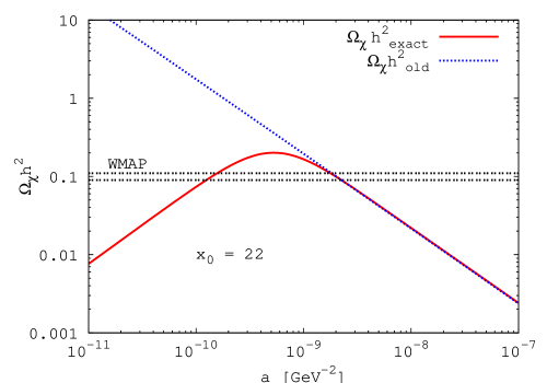
Figure 1: Predicted present relic density $\Omega_{\chi}h^{2}$ as function of the $a$ and $b$ contributions to the total cross section, see Eq.(5); in frame (a), $b=0$ whereas in (b), $a=0$. We consider two extreme cases: $\chi$ particles were in full thermal equilibrium (dotted blue line) or the number density of $\chi$ vanished (solid red line) at $x_{0}=22$. The two horizontal double–dotted black lines correspond to the 1$\sigma$ upper and lower bounds of the dark matter abundance [20].

Figure 1 shows that the relic density can be reduced if the particles never reach thermal equilibrium because of the low reheat temperature after inflation. The solid red curves depict the predicted present relic density $\Omega_{\chi}h^{2}$ as function of $a$ (a) and $b$ (b) defined in Eq.(5). Here we assume that the relic abundance vanished at the initial temperature of $x_{0}=22$, which is around the typical WIMP decoupling temperature. Here, as well as in the subsequent figures, the “exact” numerical solution of the Boltzmann equation (14) has been obtained using the Runge–Kutta algorithm, with a step size that increases quickly with increasing $x-x_{0}$. For large cross section we observe $\Omega_{\chi}h^{2}\propto 1/\langle\sigma v\rangle$, in accord with the “standard” prediction (11). However, when the cross section is reduced, the relic density reaches a maximum, and then decreases $\propto\langle\sigma v\rangle$. For the given choice of initial conditions, there are therefore two distinct ranges in $\langle\sigma v\rangle$ where the relic density comes out in the desired range [20].

In the following we attempt to find a convenient analytic formula applicable even to low temperature scenarios. As zeroth order solution of Eq.(14) we consider the case where $\chi$ annihilation is completely negligible,

$$\frac{dY_{0}}{dx}=fc(ax+6b)\,{\rm e}^{-2x}\,.$$ (16)

This equation can easily be integrated, giving

$$Y_{0}(x)=fc\left[\frac{a}{2}(x_{0}{\rm e}^{-2x_{0}}-x{\rm e}^{-2x})+\left(\frac{a}{4}+3b\right)({\rm e}^{-2x_{0}}-{\rm e}^{-2x})\right]+Y_{\chi}(x_{0})\,.$$ (17)

For $x\gg x_{0}$, the relic abundance of the particles becomes constant,

$$Y_{0,\infty}\equiv Y_{0}(x\gg x_{0})=fc\left[\frac{a}{2}x_{0}{\rm e}^{-2x_{0}}+\left(\frac{a}{4}+3b\right){\rm e}^{-2x_{0}}\right]+Y_{\chi}(x_{0})\,.$$ (18)

The corresponding prediction for the present relic density is given by

$$\Omega_{\chi}h^{2}=2.8\times 10^{8}~{}m_{\chi}Y_{0,\infty}~{}\mbox{GeV}^{-1}\,.$$ (19)

Notice that the relic density is proportional to the cross section, although the coefficient of proportionality depends on whether $a$ or $b$ is dominant.

So far no analytic solution has been known for the in–between case where both annihilation and production play a crucial role in determining the relic abundance while thermal equilibrium is not fully achieved. We now attempt to connect the standard scenario ($T_{R}>T_{F}$) and the low reheat temperature scenario ($T_{R}<T_{F}$) using some analytic method.

Since we already have the solution only including the production term, the most natural extension is to add a correction term which describes the effect of annihilation on the solution for the pure production case:

$$Y_{1}=Y_{0}+\delta\,.$$ (20)

By definition $\delta$ vanishes at the initial temperature. Since it describes the effect of $\chi$ annihilation, it is negative for $x>x_{0}$. As long as $|\delta|$ is small compared to $Y_{0}$, the evolution equation for $\delta$ is given by

$$\frac{d\delta}{dx}=-f\left(a+\frac{6b}{x}\right)\frac{Y_{0}(x)^{2}}{x^{2}}\,.$$ (21)

Using Eq.(17) for $Y_{0}(x)$, this can again be integrated:

$$\delta(x) = -f^{3}c^{2}\left[\frac{1}{4}a^{3}F^{4}_{0}(x,x_{0})+\frac{1}{4}a^{2}(a+18b)F^{4}_{1}(x,x_{0})\right.$$ (22)

$$\hskip 34.1433pt\left.+\frac{1}{16}a(a+12b)(a+36b)F^{4}_{2}(x,x_{0})+\frac{3}{8}b(a+12b)^{2}F^{4}_{3}(x,x_{0})\right]$$

$$+ Y_{0,\infty}f^{2}c\left[a^{2}F^{2}_{1}(x,x_{0})+\frac{1}{2}a(a+24b)F^{2}_{2}(x,x_{0})+3b(a+12b)F^{2}_{3}(x,x_{0})\right]$$

$$- Y_{0,\infty}^{2}f\left[aF^{0}_{2}(x,x_{0})+6bF^{0}_{3}(x,x_{0})\right]\,,$$

where

$$F^{m}_{n}(x,x_{0})=\int_{x_{0}}^{x}dt\ \frac{{\rm e}^{-mt}}{t^{n}}\,,\quad m=0,2,4\,,\quad n=1,2,3\,.$$ (23)

The functions $F^{m}_{n}(x,x_{0})$ can be expressed analytically in terms of the exponential integral of first order E${}_{1}(x)$; a complete list of the relevant $F_{n}^{m}$ is given in the Appendix, Eqs.(Appendix). At late times, $x\rightarrow\infty$, this simplifies to

$$\delta(x\to\infty) = -f^{3}c^{2}{\rm e}^{-4x_{0}}\left[\frac{a^{3}}{4}x_{0}+\frac{a^{2}(a+60b)}{16}-\frac{9ab(a-16b)}{8x_{0}}\right.$$ (24)

$$\hskip 56.9055pt\left.+\frac{9b(5a^{2}-56ab+96b^{2})}{32x_{0}^{2}}\right]~{}$$

$$- f^{2}c{\rm e}^{-2x_{0}}Y_{\chi}(x_{0})\left[a^{2}+\frac{9ab}{x_{0}}-\frac{9b(a-4b)}{2x_{0}^{2}}\right]$$

$$- f(Y_{\chi}(x_{0}))^{2}\left(\frac{a}{x_{0}}+\frac{3b}{x_{0}^{2}}\right)\,,$$

where we omit higher order terms than ${\cal O}(1/x_{0}^{2})$. Notice that we discard ${\cal O}(1/x^{2})$ and ${\cal O}(1/x^{3})$ terms in $\langle\sigma v\rangle$, which also contribute to higher order terms in Eq.(24). If $a\neq 0$ we therefore expect additional terms ${\cal O}(1/x_{0})$ from terms not included in Eq.(5); if $a=0$, higher order terms in the expansion of the cross section only contribute at ${\cal O}(1/x_{0}^{3})$ in Eq.(24).

Since, for vanishing initial abundance, $Y_{0}$ is proportional to the cross section $\sigma$, $\delta$ is proportional to $\sigma^{3}$. On the other hand, for sufficiently large cross section we want to recover the standard expression, where $Y_{\chi}(x\rightarrow\infty)\propto 1/\langle\sigma v\rangle$. This suggests to rewrite our ansatz (20) as

$$Y_{1}=Y_{0}+\delta=Y_{0}\left(1+\frac{\delta}{Y_{0}}\right)\simeq\frac{Y_{0}}{1-\delta/Y_{0}}\equiv Y_{1,r}\,.$$ (25)

Although the final approximate equality in Eq.(25) only holds for $|\delta|\ll Y_{0}$, we note that the resulting expression has the right behavior, $Y_{1,r}\propto 1/\sigma$, for large cross section. In the following we will show that this “resummation” of the correction $\delta$ is indeed able to describe the relic density for a wide range of cross sections and temperatures, including scenarios where the standard treatment is applicable.

In fact, this ansatz solves the Boltzmann equation (14) exactly in the simple case where thermal $\chi$ production can be ignored, but $Y_{\chi}(x_{0})$ is sizable, leading to significant $\chi$ annihilation. In this case Eq.(14) reduces to

$$\frac{dY_{\chi}}{dx}=-f\left(a+\frac{6b}{x}\right)\frac{Y_{\chi}^{2}}{x^{2}}\,.$$ (26)

This equation can easily be solved analytically. The solution decreases monotonically from its initial value $Y_{\chi}(x_{0})$:

$$Y_{\chi}=\frac{Y_{\chi}(x_{0})}{1+fY_{\chi}(x_{0})\left[a(1/x_{0}-1/x)+3b(1/x_{0}^{2}-1/x^{2})\right]}\,.$$ (27)

In order to treat this case using the formalism of Eqs.(16)–(25), we simply drop all terms which depend exponentially on $x$ or $x_{0}$; these terms come from thermal $\chi$ production, and are obviously very small for sufficiently small initial temperature. The zeroth order solution (17) then obviously reduces to the constant $Y_{\chi}(x_{0})$, and the correction $\delta$ of Eq.(22) simplifies to

$$\delta(x) \rightarrow -f\left(Y_{\chi}(x_{0})\right)^{2}\left[aF_{2}^{0}(x,x_{0})+6bF_{3}^{0}(x,x_{0})\right]$$ (28)

$$= -f\left(Y_{\chi}(x_{0})\right)^{2}\left[a\left(\frac{1}{x_{0}}-\frac{1}{x}\right)+3b\left(\frac{1}{x_{0}^{2}}-\frac{1}{x^{2}}\right)\right]\,;$$

in the last step we have used the last two Eqs.(Appendix). Inserting this in the last expression in Eq.(25), we indeed recover the exact solution (27), as advertised.

In principle, we can add further correction terms to the first order approximation of Eq.(20),

$$Y_{\chi}=Y_{0}+\delta+\delta_{2}+\delta_{3}+\cdots\,.$$ (29)

The above discussion shows that this corresponds to an expansion in powers of $\langle\sigma v\rangle$. Since $Y_{0}>0$ and $\delta<0$ by definition, the systematic expansion will lead to an alternating series which possesses good convergence properties. However, this type of expansion is quite cumbersome because $|\delta|$ often dominates over $Y_{0}$ for not very small cross sections, as we will explicitly see later. Therefore the re–summed ansatz $Y_{1,r}$ of Eq.(25) is much more convenient. We will see that it often provides a good approximation to the exact solution even if thermal $\chi$ production is not negligible.

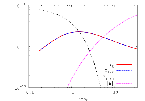
Figure 2: Evolution of the exact solution $Y_{\chi}$ (solid red curves), $Y_{1,r}$ of Eq.(25) (dotted blue), the equilibrium density $Y_{\chi,{\rm eq}}$ of Eq.(2) (double–dotted black), and $|\delta|$ of Eq.(22) (short–dashed violet) as function of $x-x_{0}$. The initial abundance is assumed to be $Y_{\chi}(x_{0}=22)=0$. We take (a) $a=10^{-9}$ GeV^-2, $b=0$, (b) $a=10^{-8}$ GeV^-2, $b=0$, (c) $a=0$, $b=10^{-8}$ GeV^-2, and (d) $a=0$, $b=10^{-7}$ GeV^-2. In frames (a) and (c) the curves for $Y_{1,r}$ practically coincide with the solid lines.

In Fig. 2 we present the evolution of the exact, numerical solution $Y_{\chi}$ (solid red), $Y_{1,r}$ (dotted blue), $Y_{\chi,{\rm eq}}$ (double–dotted black) and $|\delta|$ (short–dashed violet) as function of $x-x_{0}$. Here we consider vanishing initial $\chi$ density, $Y_{\chi}(x_{0}=22)=0.$ Clearly the first order approximation $Y_{1}$ of Eq.(20) fails to reproduce the exact result once $|\delta|$ becomes comparable to $Y_{0}$. On the contrary, frames (a) and (c) show that the re–summed ansatz $Y_{1,r}$ of Eq.(25) reproduces the numerical solution very well for all $x>x_{0}$ if $a\raisebox{-3.69899pt}{~{}\shortstack{$<$ \\ [-0.07cm] $\sim$}}~{}10^{-9}$ GeV^-2 and $b\raisebox{-3.69899pt}{~{}\shortstack{$<$ \\ [-0.07cm] $\sim$}}~{}10^{-8}$ GeV^-2. However, for intermediate values of $x-x_{0}$, the disagreement between $Y_{1,r}$ and the exact solution becomes large as the cross section increases. In frames (b) and (d) of Fig. 2 sizable deviations from the exact value are observed at $x-x_{0}\sim 1$ for $a=10^{-8}$ GeV^-2 or $b=10^{-7}$ GeV^-2. For larger $x$ the deviation becomes smaller again, and for $x\gg x_{0}$ the difference is insignificant even for these large cross sections.

We also analyzed scenarios with sizable initial $\chi$ abundance, $Y_{\chi}(x_{0})\neq 0$. Figure 3 shows that the re–summed ansatz again matches the numerical result very well for all values of $x$ if $a\raisebox{-3.69899pt}{~{}\shortstack{$<$ \\ [-0.07cm] $\sim$}}~{}10^{-9}$ GeV^-2. This is not surprising since, as we saw in the discussion of Eq.(28), it reproduces the exact solution if $Y_{\chi}(x_{0})$ dominates over the thermal contribution. For $a=10^{-8}$ GeV^-2, $Y_{1,r}$ again starts to deviate from the exact numerical solution at $x\sim 0.1$, but approaches it for $x\gg x_{0}$. Note also that already for the smaller cross section chosen in this Figure, the final relic density is almost independent of $Y_{\chi}(x_{0})$.

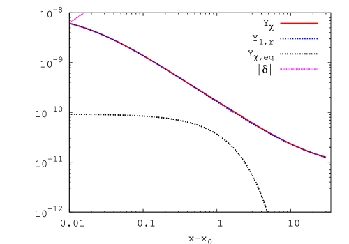
Figure 3: Evolution of $Y_{\chi}$ (solid red curves), $Y_{1,r}$ (dotted blue), $Y_{\chi,{\rm eq}}$ (double–dotted black) and $|\delta|$ (short–dashed violet) as function of $x-x_{0}$. Here we take (a) $a=10^{-9}$ GeV^-2, $Y_{\chi}(x_{0})=10^{-8}$, (b) $a=10^{-9}$ GeV^-2, $Y_{\chi}(x_{0})=10^{-10}$, (c) $a=10^{-8}$ GeV^-2, $Y_{\chi}(x_{0})=10^{-7}$ and (d) $a=10^{-8}$ GeV^-2, $Y_{\chi}(x_{0})=10^{-10}$. The other parameters are as in Fig. 2.

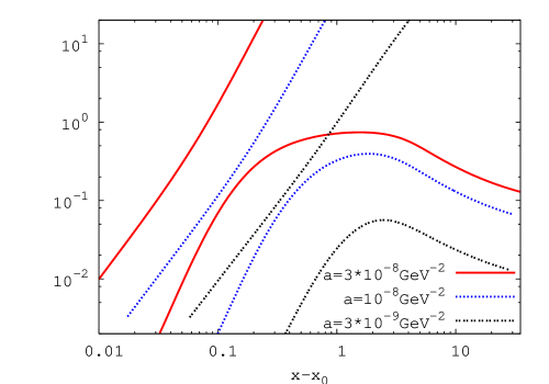
Figure 4: Evolution of $|\delta|/Y_{\chi}$ (upper curves) and $\epsilon/Y_{\chi}$ (lower curves) as function of $x-x_{0}$ for $a=3\times 10^{-8}$ GeV^-2 (solid red), $a=10^{-8}$ GeV^-2 (dotted blue) and $a=3\times 10^{-9}$ GeV^-2 (double–dotted black). Here we choose $b=0$ and $Y_{\chi}(x_{0}=22)=0$.

Let us take a closer look at the difference between the exact solution and the re–summed ansatz. To this end, we define the deviation $\epsilon$ by

$$Y_{\chi}=\frac{Y_{0}}{1-\delta/Y_{0}}+\epsilon\,.$$ (30)

Inserting this ansatz into the Boltzmann equation (4) leads to the evolution equation for $\epsilon$:

$$\frac{d\epsilon}{dx}=-\frac{f\langle\sigma v\rangle}{x^{2}}\left[\epsilon^{2}+2\epsilon\ \frac{Y_{0}}{1-\delta/Y_{0}}-\frac{(\delta/Y_{0})^{2}}{(1-\delta/Y_{0})^{2}}\ Y_{\chi,{\rm eq}}^{2}\right]\,,$$ (31)

which again resembles the Boltzmann equation. Since initially $\epsilon=0$, our re–summed ansatz works very well as long as $\delta/Y_{0}$ remains suppressed. Note that the inhomogeneous term on the rhs of Eq.(31) is of order $(\delta/Y_{0})^{2}$. The analogous correction to our original first order solution $Y_{1}$ of Eq.(20) would start at ${\cal O}(\delta/Y_{0})$. Since this inhomogeneous term is positive, $\epsilon(x)>0$ for all $x>x_{0}$, i.e. $Y_{1,r}$, like $Y_{1}$, always under–estimates the exact solution. As $|\delta|/Y_{0}$ grows, the last term in Eq.(31) can become sizable. Note, however, that it is multiplied with $\left(Y_{\chi,{\rm eq}}\right)^{2}$, which drops $\propto\exp{(-2x)}$ with increasing $x$. Therefore $\epsilon$ becomes large only if $|\delta|$ reaches values of order of $Y_{0}$ for $x-x_{0}\raisebox{-3.69899pt}{~{}\shortstack{$<$ \\ [-0.07cm] $\sim$}}~{}1$. The homogeneous terms in Eq.(31) imply that for large $x-x_{0}$ the deviation $\epsilon$ decreases again, similar to the WIMP relic abundance $Y_{\chi}$. This situation is depicted in Fig. 4, which shows the evolutions of $|\delta|/Y_{\chi}$ (upper curves) and $\epsilon/Y_{\chi}$ (lower curves) as function of $x-x_{0}$ for $a=3\times 10^{-8}$ GeV^-2 (solid red), $a=10^{-8}$ GeV^-2 (dotted blue) and $a=3\times 10^{-9}$ GeV^-2 (double–dotted black). Here we choose $b=0$ and $Y_{\chi}(x_{0}=22)=0$. Even in the case where $\epsilon$ becomes sizable for intermediate values of $x$, it eventually diminishes and hence our analytical formula succeeds in reproducing the present relic abundance $Y_{\chi}(x\rightarrow\infty)$ fairly well.

Let us turn to a discussion of the dependence of the present relic abundance on the initial temperature. In Fig. 5 we plot the present relic density evaluated numerically (solid red curves), the old standard approximation (dotted blue) and our new approximation (double–dotted black) as function of $x_{0}$. Here we take (a) $a=10^{-8}$ GeV^-2, $b=0$ and (b) $a=10^{-9}$ GeV^-2, $b=0$. We find that our approximation agrees with the exact result very well for $x_{0}>x_{F}$. On the other hand, for $x_{0}<x_{F}$, our approximation gives too small an abundance while the old approximation works very well. The transition between the two regimes is very sharp. For $x_{0}=x_{F}+2$, the old approximation over–estimates the relic abundance by as much as an order of magnitude, while for $x_{0}=x_{F}$ both the old and the new approximation work well.

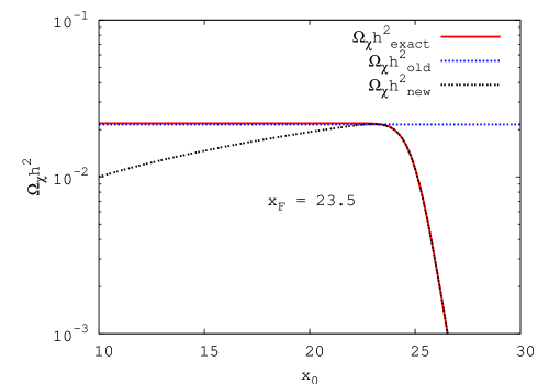
Figure 5: The present relic density evaluated numerically (solid red curves), the old standard approximation (dotted blue) and our new approximation (double–dotted black) as function of $x_{0}$. Here we take (a) $a=10^{-8}$ GeV^-2, $b=0$ and (b) $a=10^{-9}$ GeV^-2, $b=0$.

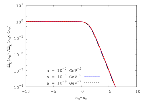
Figure 6: $\Omega_{\chi}(x_{0})/\Omega_{\chi}(x_{0}\ll x_{F})$ as function of $x_{0}-x_{F}$. In the left frame, $a=10^{-7}$ GeV^-2 (solid red curves), $10^{-8}$ GeV^-2 (dotted blue) and $10^{-9}$ GeV^-2 (double–dotted black) with $b=0$, whereas in the right frame, $b=10^{-6}$ GeV^-2 (solid red), $10^{-7}$ GeV^-2 (dotted green) and $10^{-8}$ GeV^-2 (double–dotted black) with $a=0$.

We found that for vanishing initial $\chi$ density, $Y_{\chi}(x_{0})=0$, different values of the cross section lead to a universal behavior when the present relic density is expressed as function of $x_{0}-x_{F}$ and in units of the relic density for $x_{0}\ll x_{F}$. This can be seen from the analytic solution we have obtained. For $x_{0}\ll x_{F}$ it is obvious that $\Omega_{\chi}(x_{0})/\Omega_{\chi}(x_{0}\ll x_{F})$ is nothing but unity and independent of the cross section. For $x_{0}\gg x_{F}$, the exact solution is roughly given by the zeroth order approximation $Y_{0}$, which scales like $a{\rm e}^{-2x_{0}}$ if $a$ dominates and the initial abundance vanishes. Meanwhile, Eq.(13) shows that $x_{F}$ is roughly proportional to $\ln a$. Therefore we obtain the relation

$$\frac{\Omega_{\chi}(x_{0})}{\Omega_{\chi}(x_{0}\ll x_{F})}\propto\frac{a{\rm e}^{-2x_{0}}}{1/a}\propto{\rm e}^{-2(x_{0}-x_{F})}\,,$$ (32)

which has no explicit dependence on the cross section. The same argument is applicable to the case where $b$ is dominant. In Fig. 6 we plot the ratio of the exact present relic density to the value for $x_{0}\ll x_{F}$, $\Omega_{\chi}(x_{0})/\Omega_{\chi}(x_{0}\ll x_{F})$, as function of $x_{0}-x_{F}$ for various values of $a$ and $b$. These figures clearly show the expected scaling behavior both for $a\neq 0,\,b=0$ (left frame) and for $a=0,\,b\neq 0$ (right frame). However, for $Y_{\chi}(x_{0})\neq 0$, no such scaling exists, apart from the fairly obvious result that $Y_{\chi}(x\gg x_{0})$ becomes independent of $Y_{\chi}(x_{0})$ if $x_{0}\ll x_{F}$.

Fig. 5 shows that $Y_{1,r}(x_{0},x\rightarrow\infty)$ has a well defined maximum when $x_{0}$ is varied. This maximum occurs at a value $x_{0,{\rm max}}$ which is close, but not identical, to the decoupling temperature $x_{F}$ of Eq.(13). From the asymptotic expressions for $Y_{0}$, Eq.(18), and $\delta$, Eq.(24), we find for $Y_{\chi}(x_{0})=0$:

$$x_{0,{\rm max}} \simeq \frac{1}{2}\ln\frac{f^{2}c(a+6b/x_{0,{\rm max}})^{2}}{4x_{0,{\rm max}}}$$ (33)

$$= \ln\frac{0.096\ m_{\chi}M_{\rm Pl}g_{\chi}(a+6b/x_{0,{\rm max}})}{\sqrt{x_{0,{\rm max}}g_{*}}}\,.$$

In deriving this equation, we neglect non–leading terms in $1/x_{0,{\rm max}}$ in each combination of $a$ and $b$. Notice that $x_{0,{\rm max}}$ coincides with $x_{F}$ of Eq.(13), if one chooses $\xi=1/4$ (rather than $\xi=\sqrt{2}-1$).

Since the actual relic density is already practically independent of $x_{0}$ for $x_{0}<x_{0,{\rm max}}$ we can construct a new semi-analytic solution which describes the relic density for the whole range of $x_{0}$: for $x_{0}>x_{0,{\rm max}}$, compute the relic density from $Y_{1,r}(x_{0})$, but for $x_{0}<x_{0,{\rm max}}$, use $Y_{1,r}(x_{0,{\rm max}})$ instead.

The ratio of this semi–analytic result $\Omega_{1,r}$ to the exact value $\Omega_{\chi}$ is depicted in Fig. 7. As noted earlier, our approximation becomes exact for $x_{0}\raisebox{-3.69899pt}{~{}\shortstack{$>$ \\ [-0.07cm] $\sim$}}~{}x_{F}$. For smaller $x_{0}$ the new approximation still slightly under–estimates the correct answer, but the deviation is at most $1.7$% for $b=0$ (left frame), and $3.0$% for $a=0$ (right frame). On the other hand, in the same region the old standard approximation reproduces the present relic abundance within 1% error. We thus see that for $x_{0}<x_{F}$, this new expression works nearly as well as the old standard result; of course, the old result fails badly for $x_{0}>x_{F}$. Finally, since by definition $Y_{1,r}$ depends only weakly on $x_{0}$ for $x_{0}\sim x_{0,{\rm max}}$, the latter quantity need not be calculated very precisely; in practice, setting $x_{0,{\rm max}}=20$ in the rhs of Eq.(33) is often sufficient. In contrast, the standard approximation (11) depends linearly (for $b=0$) or even quadratically (for $a=0$) on $x_{F}$; several iterations are therefore required to solve Eq.(13) to sufficient accuracy. Altogether, our new semi–analytic formula is evidently a quite powerful tool in calculating the density of cold relics.

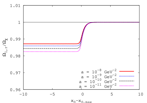
Figure 7: Ratios of approximate and exact results for the relic density $\Omega_{1,r}/\Omega_{\chi}$ as function of $x_{0}-x_{0,{\rm max}}$, for $a\neq 0,\,b=0$ (left frame) and $a=0,b\neq 0$ (right frame). The curves use $Y_{1,r}$ with $x_{0}$ replaced by $\max(x_{0},\,x_{0,{\rm max}})$, see Eq.(33). In the left frame, $a=10^{-8}$ GeV^-2 (solid red curves), $10^{-9}$ GeV^-2 (dotted blue), $10^{-10}$ GeV^-2 (double–dotted black), $10^{-11}$ GeV^-2 (short–dashed violet) with $b=0$, whereas in the right frame, $b=10^{-7}$ GeV^-2 (solid red), $10^{-8}$ GeV^-2 (dotted blue), $10^{-9}$ GeV^-2 (double–dotted black), $10^{-10}$ GeV^-2 (short–dashed violet) with $a=0$.

4 Relic Abundance Including the Decay of Heavier Particles

In this section we investigate a scenario where unstable heavy particles $\phi$ decay into long–lived or stable particles $\chi$. We assume that $\phi$ decays out of thermal equilibrium, so that $\phi$ production is negligible; however, we include both thermal and non–thermal production of $\chi$ particles. For example in some supersymmetric models neutralinos, which are stable due to R–parity, can be produced non–thermally through the decay of moduli [21] or gravitinos after the end of inflation. The number densities of $\chi$ and $\phi$ obey the following coupled Boltzmann equations:

$$\frac{dn_{\chi}}{dt}+3Hn_{\chi} = -\langle\sigma v\rangle(n_{\chi}^{2}-n_{\chi,{\rm eq}}^{2})+N\Gamma_{\phi}n_{\phi}\,,$$

$$\frac{dn_{\phi}}{dt}+3Hn_{\phi} = -\Gamma_{\phi}n_{\phi}\,,$$ (34)

where $N$ is the average number of $\chi$ particles produced in a $\phi$ decay, and $\Gamma_{\phi}$ and $n_{\phi}$ are the decay rate and the number density of the heavier particle. In contrast to refs.[12] we assume that $\phi$ does not dominate the total energy density, so that the co–moving entropy density remains approximately constant throughout. The Boltzmann equation for $n_{\phi}$ can then easily be solved analytically, using the fact that $t\propto T^{-2}\propto x^{2}$ in the radiation–dominated era. Inserting this solution into the equation for $n_{\chi}$, and again switching variables to $Y_{\chi}=n_{\chi}/s$, $Y_{\phi}=n_{\phi}/s$ and $x$, the Boltzmann equation for $\chi$ becomes

$$\frac{dY_{\chi}}{dx}=-\frac{\langle\sigma v\rangle s}{Hx}(Y_{\chi}^{2}-Y_{\chi,{\rm eq}}^{2})+NrxY_{\phi}(x_{0})\exp\left(-\frac{r}{2}(x^{2}-x_{0}^{2})\right)\,,$$ (35)

where $r=\Gamma_{\phi}/Hx^{2}=(\Gamma_{\phi}M_{\rm Pl}/\pi m_{\chi}^{2})\sqrt{90/g_{*}}$ is constant. The zeroth order solution of Eq.(35) is again obtained by neglecting $\chi$ annihilation. Using the expansion (5) of the annihilation cross section, we have

$$\frac{dY_{0}}{dx}=f\left(a+\frac{6b}{x}\right)cx{\rm e}^{-2x}+NrxY_{\phi}(x_{0})\exp\left(-\frac{r}{2}(x^{2}-x_{0}^{2})\right)\,.$$ (36)

This equation can be integrated, giving

$$Y_{0} = fc\left[\frac{a}{2}(x_{0}{\rm e}^{-2x_{0}}-x{\rm e}^{-2x})+\left(\frac{a}{4}+3b\right)({\rm e}^{-2x_{0}}-{\rm e}^{-2x})\right]$$ (37)

$$+ NY_{\phi}(x_{0})\left[1-\exp\left(-\frac{r}{2}(x^{2}-x_{0}^{2})\right)\right]+Y_{\chi}(x_{0})\,.$$

For $x\gg x_{0}$, $Y_{0}$ becomes constant,

$$Y_{0,\infty}=fc\left[\frac{a}{2}x_{0}{\rm e}^{-2x_{0}}+\left(\frac{a}{4}+3b\right){\rm e}^{-2x_{0}}\right]+NY_{\phi}(x_{0})+Y_{\chi}(x_{0})\,.$$ (38)

For sufficiently large $Y_{0}$ the annihilation term in Eq.(35) becomes significant. We add a correction term to include this effect, as in Eq.(20). Since the new, non–thermal contribution to $\chi$ production is already fully included in $Y_{0}$, the Boltzmann equation for $\delta$ is again given by Eq.(21). Using now Eq.(37) for $Y_{0}$, we can integrate Eq.(21), giving

$$\delta = \left\{-f^{3}c^{2}\left[\frac{1}{4}a^{3}F^{4}_{0}(x,x_{0})+\frac{1}{4}a^{2}(a+18b)F^{4}_{1}(x,x_{0})\right.\right.$$

$$\hskip 39.83385pt\left.+\frac{1}{16}a(a+12b)(a+36b)F^{4}_{2}(x,x_{0})+\frac{3}{8}b(a+12b)^{2}F^{4}_{3}(x,x_{0})\right]$$

$$+Y_{0,\infty}f^{2}c\left[a^{2}F^{2}_{1}(x,x_{0})+\frac{1}{2}a(a+24b)F^{2}_{2}(x,x_{0})+3b(a+12b)F^{2}_{3}(x,x_{0})\right]$$

$$\left.-Y_{0,\infty}^{2}f\left[aF^{0}_{2}(x,x_{0})+6bF^{0}_{3}(x,x_{0})\right]\right.{\bigg{\}}}$$

$$- N^{2}Y^{2}_{\phi}(x_{0}){\rm e}^{rx_{0}^{2}}f[aG_{2}^{r}(x,x_{0})+6bG_{3}^{r}(x,x_{0})]$$

$$+ 2NY_{\phi}(x_{0}){\rm e}^{rx_{0}^{2}/2}Y_{0,\infty}f[aG_{2}^{r/2}(x,x_{0})+6bG_{3}^{r/2}(x,x_{0})]$$

$$- NY_{\phi}(x_{0}){\rm e}^{rx_{0}^{2}/2}f^{2}c\left[a^{2}G_{1}^{c}(x,x_{0})+\frac{1}{2}a(a+24b)G_{2}^{c}(x,x_{0})+3b(a+12b)G_{3}^{c}(x,x_{0})\right]\,.$$

The functions $G_{n}^{r}(x,x_{0})$, $G_{n}^{r/2}(x,x_{0})$ and $G_{n}^{c}(x,x_{0})$ are defined by

$$G_{n}^{r}(x,x_{0}) = \int_{x_{0}}^{x}dt\ \frac{{\rm e}^{-rt^{2}}}{t^{n}}\,,\quad n=2,3\,,$$

$$G_{n}^{r/2}(x,x_{0}) = \int_{x_{0}}^{x}dt\ \frac{{\rm e}^{-rt^{2}/2}}{t^{n}}\,,\quad n=2,3\,,$$

$$G_{n}^{c}(x,x_{0}) = \int_{x_{0}}^{x}dt\ \frac{{\rm e}^{-2t-rt^{2}/2}}{t^{n}}\,,\quad n=1,2,3\,.$$ (40)

Explicit expressions for these functions are given in the Appendix, Eqs.(Appendix). Notice that the expression in curly brackets $\{...\}$ in Eq.(4) has the same form as in Eq.(22).

Results for this scenario with $b=0$ are shown in Fig. 8. We choose $r=0.1$ so that $rx_{0}^{2}\sim x_{0}$, which leads to the most difficult situation where thermal and non–thermal production occur simultaneously. We see that even for the smaller cross section considered, $a=10^{-9}$ GeV^-2 (top frames), the simple first–order solution (20) soon fails, since $|\delta|$ exceeds $Y_{0}$. However, the re–summed ansatz $Y_{1,r}$ of Eq.(25) describes the exact temperature dependence very well for this cross section, both for large (top left frame) and moderate (top right) non–thermal $\chi$ production. For $a=10^{-8}$ GeV^-2 (bottom frames) we again observe sizable deviations for intermediate values of $x-x_{0}$.

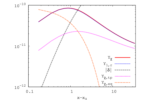
Figure 8: Evolution of $Y_{\chi}$ (solid red curves), $Y_{1,r}$ (dotted blue), $|\delta|$ (double–dotted black), the prediction for purely thermal $\chi$ production $Y_{\chi,{\rm tp}}$ (short–dashed violet) and $Y_{\rm eq}$ (triple–dotted orange) as function of $x-x_{0}$, for $Y_{\chi}(x_{0}=22)=0$, $r=0.1$, $N=1$ and $b=0$. The $S-$wave cross section and the initial $\phi$ density are (a) $a=10^{-9}$ GeV^-2, $Y_{\phi}(x_{0})=10^{-10}$, (b) $a=10^{-9}$ GeV^-2, $Y_{\phi}(x_{0})=10^{-11}$, (c) $a=10^{-8}$ GeV^-2, $Y_{\phi}(x_{0})=10^{-9}$ and (d) $a=10^{-8}$ GeV^-2, $Y_{\phi}(x_{0})=10^{-10}$.

In fact, comparison with Fig. 2 shows that non–thermal $\chi$ production leads to faster growth of $|\delta|$, and hence to earlier and larger deviation between $Y_{1,r}$ and the exact solution of the Boltzmann equation (35). However, comparison with the curves labeled $Y_{\chi,{\rm tp}}$, where non–thermal $\chi$ production is neglected, show that for this rather large cross section and short $\phi$ lifetime, the non–thermal production mechanism does not affect the final $\chi$ relic density any more. This agrees with the result of Fig. 3, where we saw that for the same values of $a$ and $x_{0}$, the relic density is independent of the initial value $Y_{\chi}(x_{0})$. As before, $Y_{1,r}$ approaches the exact result again for $x-x_{0}\gg 1$. We therefore conclude that our re–summed ansatz describes scenarios with additional non–thermal $\chi$ production as well as the simpler case with only thermal production.

5 Summary and Conclusions

In this paper we investigated the relic abundance of non–relativistic long–lived or stable particles $\chi$ using analytical as well as numerical methods. Our emphasis was on scenarios with low re–heat temperature, so that $\chi$ may never have been in full thermal equilibrium after the end of inflation. Such scenarios are interesting because they lower the predicted relic abundance and therefore open the parameter space of particle physics models, allowing combinations of parameters which are cosmologically disfavored in the standard high temperature scenario.

The case of small $\chi$ annihilation cross section or very low temperature can easily be treated analytically, since in this case $\chi$ annihilation can either be ignored completely, leading to our zeroth order solution $Y_{0}$ of Eq.(17), or can be treated as small perturbation, as in our first order solution $Y_{1}$ of Eq.(20). Unfortunately this approximation breaks down well before $\chi$ attains full thermal equilibrium. On the other hand, we found that the simple trick of “re–summing” the correction due to $\chi$ annihilation, as in Eq.(25), allows to describe the full temperature dependence of the $\chi$ number density as long as $\chi$ does not reach full equilibrium. We saw in Sec. 4 that this remains true even if a non–thermal source of $\chi$ production is added. Our ansatz therefore provides a first analytical description of the “in–between” situation, where $\chi$ annihilation is very significant but not large enough to establish full chemical equilibrium with the thermal plasma.

For yet higher cross sections or temperatures even the re–summed ansatz fails to describe the temperature dependence of the $\chi$ number density at intermediate temperatures. However, by replacing the initial scaled inverse temperature $x_{0}$ with the quantity $x_{0,{\rm max}}$ of Eq.(33) our ansatz succeeds in predicting the final relic density about as well as the standard semi–analytical high temperature treatment does, with comparable numerical effort.

In this paper we have used the non–relativistic expansion of the $\chi$ annihilation cross section. This expansion is known to fail in certain cases even for non–relativistic WIMPs [6]. We expect our methods to be applicable to these situations as well. However, a full analytical treatment will be possible only if the product of thermally averaged cross section and squared $\chi$ equilibrium number density, expressed as function of the scaled inverse temperature $x$, can be integrated analytically over $x$.

From the particle physics point of view, the main effect of a low reheat temperature is that it allows to reproduce the correct relic density in scenarios with low annihilation cross section, e.g. for Bino–like neutralinos and large sfermion masses. Conversely, the non–thermal production mechanism studied in Sec. 4 allows to reproduce the correct relic density for WIMPs with large annihilation cross section, e.g. Wino–like neutralinos [21]. As noticed in [13], the combination of these effects in principle allows to completely decouple the WIMP relic density from its annihilation cross section. In many studies of expected WIMP detection rates scenarios yielding too high a relic density under the standard assumptions were not considered; such scenarios typically also lead to low detection rates. Conversely, in scenarios leading to too low a thermal WIMP density, which typically predict large detection rates for fixed WIMP density, the predicted detection rates were often rescaled by the ratio of the predicted to the observed relic density. If one allows lower reheat temperatures and/or non–thermal WIMP sources the possible range of signals for WIMP detection can therefore be enlarged towards both larger and smaller values.

In summary, we found analytical or semi–analytical solutions of the Boltzmann equation describing the density of non–relativistic relics which are valid for a wide range of initial conditions. In particular, they allow a complete description of the temperature dependence for small or moderate cross sections, and correctly reproduce the final relic density for all combinations of initial temperature and cross section. This should be a powerful tool for exploring the physics of non–relativistic relics, especially in scenarios with low reheat temperature.

Acknowledgments

The authors would like to thank the European Network of Theoretical Astroparticle Physics ILIAS/N6 under contract number RII3–CT–2004–506222 for financial support. The work of M.K. is supported in part by the Japan Society for the Promotion of Science.

Appendix

In this Appendix, we give explicit expressions for the functions $F^{m}_{n}(x,x_{0})$, $G_{n}^{r}(x,x_{0})$, $G_{n}^{r/2}(x,x_{0})$ and $G_{n}^{c}(x,x_{0})$ which appear in Secs. 3 and 4. These functions are analytically expressed in terms of the exponential integral of the first order ${\rm E}_{1}(x)$ and the error function ${\rm erfc}(x)$.

First we review the exponential integral and the error function. The exponential integral of the first order is defined by

$${\rm E}_{1}(x)=\int_{1}^{\infty}dt\ \frac{{\rm e}^{-xt}}{t}=\int_{x}^{\infty}dt\ \frac{{\rm e}^{-t}}{t}\,.$$ (41)

We need this function only for $x>x_{0}\gg 1$. We can then use the asymptotic large $x$ expansion,

$${\rm E}_{1}(x)\sim\frac{{\rm e}^{-x}}{x}\sum^{\infty}_{n=0}\frac{(-1)^{n}n!}{x^{n}}\,.$$ (42)

The error function is defined by

$${\rm erfc}(x) = \frac{2}{\sqrt{\pi}}\int_{x}^{\infty}dt\ {\rm e}^{-t^{2}}\,,$$ (43)

with asymptotic large $x$ expansion

$${\rm erfc}(x)\sim\frac{{\rm e}^{-x^{2}}}{\sqrt{\pi}x}\sum^{\infty}_{n=0}\frac{(-1)^{n}(2n-1)!!}{(2x^{2})^{n}}\,.$$ (44)

The functions $F^{m}_{n}(x,x_{0})$ are defined by

$$F^{m}_{n}(x,x_{0})=\int_{x_{0}}^{x}dt\ \frac{{\rm e}^{-mt}}{t^{n}}\,.$$ (45)

These integrals can be reduced to the form (41). The resulting expressions and corresponding asymptotic expansions, computed from Eq.(42), are:

$$F^{4}_{0}(x,x_{0}) = \frac{1}{4}({\rm e}^{-4x_{0}}-{\rm e}^{-4x})\,,$$

$$F^{4}_{1}(x,x_{0}) = {\rm E}_{1}(4x_{0})-{\rm E}_{1}(4x)$$

$$\sim \frac{{\rm e}^{-4x_{0}}}{4x_{0}}\left(1-\frac{1}{4x_{0}}\right)-\frac{{\rm e}^{-4x}}{4x}\left(1-\frac{1}{4x}\right)+{\cal O}\left(\frac{{\rm e}^{-4x_{0}}}{x_{0}^{3}}\right)\,,$$

$$F^{4}_{2}(x,x_{0}) = \frac{{\rm e}^{-4x_{0}}}{x_{0}}-4{\rm E}_{1}(4x_{0})-\frac{{\rm e}^{-4x}}{x}+4{\rm E}_{1}(4x)$$

$$\sim \frac{{\rm e}^{-4x_{0}}}{4x_{0}^{2}}-\frac{{\rm e}^{-4x}}{4x^{2}}+{\cal O}\left(\frac{{\rm e}^{-4x_{0}}}{x_{0}^{3}}\right)\,,$$

$$F^{4}_{3}(x,x_{0}) = \frac{{\rm e}^{-4x_{0}}}{2x_{0}^{2}}-2\frac{{\rm e}^{-4x_{0}}}{x_{0}}+8{\rm E}_{1}(4x_{0})-\frac{{\rm e}^{-4x}}{2x^{2}}+2\frac{{\rm e}^{-4x}}{x}-8{\rm E}_{1}(4x)$$

$$\sim {\cal O}\left(\frac{{\rm e}^{-4x_{0}}}{x_{0}^{3}}\right)\,,$$

$$F^{2}_{1}(x,x_{0}) = {\rm E}_{1}(2x_{0})-{\rm E}_{1}(2x)$$

$$\sim \frac{{\rm e}^{-2x_{0}}}{2x_{0}}\left(1-\frac{1}{2x_{0}}\right)-\frac{{\rm e}^{-2x}}{2x}\left(1-\frac{1}{2x}\right)+{\cal O}\left(\frac{{\rm e}^{-2x_{0}}}{x_{0}^{3}}\right)\,,$$

$$F^{2}_{2}(x,x_{0}) = \frac{{\rm e}^{-2x_{0}}}{x_{0}}-2{\rm E}_{1}(2x_{0})-\frac{{\rm e}^{-2x}}{x}+2{\rm E}_{1}(2x)$$

$$\sim \frac{{\rm e}^{-2x_{0}}}{2x_{0}^{2}}-\frac{{\rm e}^{-2x}}{2x^{2}}+{\cal O}\left(\frac{{\rm e}^{-2x_{0}}}{x_{0}^{3}}\right)\,,$$

$$F^{2}_{3}(x,x_{0}) = \frac{{\rm e}^{-2x_{0}}}{2x_{0}^{2}}-\frac{{\rm e}^{-2x_{0}}}{x_{0}}+2{\rm E}_{1}(2x_{0})-\frac{{\rm e}^{-2x}}{2x^{2}}+\frac{{\rm e}^{-2x}}{x}-2{\rm E}_{1}(2x)$$

$$\sim {\cal O}\left(\frac{{\rm e}^{-2x_{0}}}{x_{0}^{3}}\right)\,,$$

$$F^{0}_{2}(x,x_{0}) = \frac{1}{x_{0}}-\frac{1}{x}\,,$$

$$F^{0}_{3}(x,x_{0}) = \frac{1}{2x_{0}^{2}}-\frac{1}{2x^{2}}\,.$$ (46)

The functions $G_{n}^{r}(x,x_{0})$ and $G_{n}^{r/2}(x,x_{0})$ are defined by

$$G_{n}^{r}(x,x_{0}) = \int_{x_{0}}^{x}dt\ \frac{{\rm e}^{-rt^{2}}}{t^{n}}\,,\quad n=2,3\,,$$

$$G_{n}^{r/2}(x,x_{0}) = \int_{x_{0}}^{x}dt\ \frac{{\rm e}^{-rt^{2}/2}}{t^{n}}\,,\quad n=2,3\,.$$ (47)

Using Eqs.(43) and (44), we find the following explicit expressions and corresponding asymptotic expansions:

$$G_{2}^{r}(x,x_{0}) = \frac{{\rm e}^{-rx_{0}^{2}}}{x_{0}}-\sqrt{\pi r}\ {\rm erfc}(\sqrt{r}x_{0})-\frac{{\rm e}^{-rx^{2}}}{x}+\sqrt{\pi r}\ {\rm erfc}(\sqrt{r}x)$$

$$\sim \frac{{\rm e}^{-rx_{0}^{2}}}{2rx_{0}^{3}}\left(1-\frac{3}{2rx_{0}^{2}}\right)-\frac{{\rm e}^{-rx^{2}}}{2rx^{3}}\left(1-\frac{3}{2rx^{2}}\right)+{\cal O}\left(\frac{{\rm e}^{-rx_{0}^{2}}}{x_{0}(rx_{0}^{2})^{3}}\right)\,,$$

$$G_{3}^{r}(x,x_{0}) = \frac{{\rm e}^{-rx_{0}^{2}}}{2x_{0}^{2}}-\frac{r}{2}\ {\rm E}_{1}(rx_{0}^{2})-\frac{{\rm e}^{-rx^{2}}}{2x^{2}}+\frac{r}{2}\ {\rm E}_{1}(rx^{2})$$

$$\sim \frac{{\rm e}^{-rx_{0}^{2}}}{2rx_{0}^{4}}\left(1-\frac{2}{rx_{0}^{2}}\right)-\frac{{\rm e}^{-rx^{2}}}{2rx^{4}}\left(1-\frac{2}{rx^{2}}\right)+{\cal O}\left(\frac{{\rm e}^{-rx_{0}^{2}}}{x_{0}^{2}(rx_{0}^{2})^{3}}\right)\,,$$

$$G_{2}^{r/2}(x,x_{0}) = \frac{{\rm e}^{-rx_{0}^{2}/2}}{x_{0}}-\sqrt{\frac{\pi r}{2}}\ {\rm erfc}\left(\sqrt{\frac{r}{2}}x_{0}\right)-\frac{{\rm e}^{-rx^{2}/2}}{x}+\sqrt{\frac{\pi r}{2}}\ {\rm erfc}\left(\sqrt{\frac{r}{2}}x\right)$$

$$\sim \frac{{\rm e}^{-rx_{0}^{2}/2}}{rx_{0}^{3}}\left(1-\frac{3}{rx_{0}^{2}}\right)-\frac{{\rm e}^{-rx^{2}/2}}{rx^{3}}\left(1-\frac{3}{rx^{2}}\right)+{\cal O}\left(\frac{{\rm e}^{-rx_{0}^{2}}}{x_{0}(rx_{0}^{2})^{3}}\right)\,,$$

$$G_{3}^{r/2}(x,x_{0}) = \frac{{\rm e}^{-rx_{0}^{2}/2}}{2x_{0}^{2}}-\frac{r}{4}\ {\rm E}_{1}\left(\frac{rx_{0}^{2}}{2}\right)-\frac{{\rm e}^{-rx^{2}/2}}{2x^{2}}+\frac{r}{4}\ {\rm E}_{1}\left(\frac{rx^{2}}{2}\right)$$ (48)

$$\sim \frac{{\rm e}^{-rx_{0}^{2}/2}}{rx_{0}^{4}}\left(1-\frac{4}{rx_{0}^{2}}\right)-\frac{{\rm e}^{-rx^{2}/2}}{rx^{4}}\left(1-\frac{4}{rx^{2}}\right)+{\cal O}\left(\frac{{\rm e}^{-rx_{0}^{2}}}{x_{0}^{2}(rx_{0}^{2})^{3}}\right)\,.$$

In the expansion we assume that $rx_{0}^{2}\sim x_{0}$, so that the effect of non–thermal $\chi$ production is comparable to that of thermal production.

Finally, the functions $G_{n}^{c}(x,x_{0})$ are defined by

$$G_{n}^{c}(x,x_{0})=\int_{x_{0}}^{x}dt\ \frac{{\rm e}^{-2t-rt^{2}/2}}{t^{n}}\,,\quad n=1,2,3\,.$$ (49)

They appear in the “interference terms” in Eq.(4), which are important only if thermal and non–thermal contributions to $Y_{0}$ in Eq.(37) are comparable in size. Since the overall $t-$dependence of the integrand in Eq.(49) is dominated by the numerator, we can, to good approximation, evaluate these functions by replacing $t$ in the denominator by some appropriate constant $x_{c}$:

$$G_{n}^{c}(x,x_{0}) \simeq \int_{x_{0}}^{x}dt\ \frac{{\rm e}^{-2t-rt^{2}/2}}{x_{c}^{n}}$$ (50)

$$= \frac{{\rm e}^{2/r}}{x_{c}^{n}}\sqrt{\frac{\pi}{2r}}\left[{\rm erfc}\left(\frac{1}{\sqrt{2r}}(rx_{0}+2)\right)-{\rm erfc}\left(\frac{1}{\sqrt{2r}}(rx+2)\right)\right]$$

$$\sim \frac{{\rm e}^{-2x_{0}-rx_{0}^{2}/2}}{x_{c}^{n}(rx_{0}+2)}\left[1-\frac{r}{(rx_{0}+2)^{2}}\right]-\frac{{\rm e}^{-2x-rx^{2}/2}}{x_{c}^{n}(rx+2)}\left[1-\frac{r}{(rx+2)^{2}}\right]$$

$$+{\cal O}\left(\frac{{\rm e}^{-2x_{0}-rx_{0}^{2}/2}}{x_{0}^{n-1}(rx_{0}^{2})^{3}}\right)\,.$$

In our calculations in Sec. 5 we set $x_{c}=x_{0}$; this over–estimates $G_{n}^{c}$ by a few %, with negligible error in $Y_{1,r}$.

References

[1]
E.W. Kolb and M.S. Turner, The Early Universe, Addison–Wesley
(Redwood City, CA, 1990).
[2]
For a review, see G. Bertone, D. Hooper and J. Silk, Phys. Rep. 405,
279 (2005), hep–ph/0404175.
[3]
See e.g. J. L. Feng, A. Rajaraman and F. Takayama, Phys. Rev. Lett. 91,
011302 (2003), hep–ph/0302215;
K.-Y. Choi and L. Roszkowski, Plenary talk PASCOS 2005, Gyeongju, Korea,
30 May - 4 Jun 2005, hep–ph/0511003; and references therein.
[4]
S. Sarkar, Rep. Prog. Phys. 59, 1493 (1996), hep–ph/9602260;
D. Tytler, J.M. O’Meara, N. Suzuki and D. Lubin, Phys. Scripta T85, 12
(2000), astro–ph/0001318.
[5]
R.J. Scherrer and M.S. Turner, Phys. Rev. D33, 1585 (1986),
Erratum-ibid. D34, 3263 (1986).
[6]
K. Griest and D. Seckel, Phys. Rev. D43, 3191 (1991).
[7]
R.J. Scherrer and M.S. Turner, Phys. Rev. D31, 681 (1985);
G. Lazarides, R.K. Schaefer, D. Seckel and Q. Shafi, Nucl. Phys. B346,
193 (1990);
J.E. Kim, Phys. Rev. Lett. 67, 3465 (1991).
[8]
For a review, see e.g. D.H. Lyth and A. Riotto, Phys. Rep. 314, 1
(1999), hep–ph/9807278.
[9]
G.F. Giudice, E.W. Kolb and A. Riotto, Phys. Rev. D64, 023508 (2001),
hep–ph/0005123.
[10]
S. Hannestad, Phys. Rev. D70, 043506 (2004), astro–ph/0403291;
K. Ichikawa, M. Kawasaki and F. Takahashi, Phys. Rev. D72, 043522
(2005), astro–ph/0505395.
[11]
N. Fornengo, A. Riotto and S. Scopel, Phys. Rev. D67, 023514 (2003),
hep–ph/0208072.
[12]
M. Bastero-Gil and S.F. King, Phys. Rev. D63 123509 (2001),
hep–ph/0011385;
A. Kudo and M. Yamaguchi, Phys. Lett. B516, 151 (2001),
hep–ph/0103272.
[13]
G. Gelmini and Gondolo, hep–ph/0602230.
[14]
D.J.H. Chung, E.W. Kolb and A. Riotto, Phys. Rev. D60, 063504 (1999),
hep–ph/9809453.
[15]
R. Allahverdi and M. Drees, Phys. Rev. D66, 063513 (2002),
hep–ph/0205246.
[16]
C. Pallis, Astropart. Phys. 21, 689 (2004), hep–ph/0402033.
[17]
J.H. Traschen and R.H. Brandenberger, Phys. Rev. D42, 2491 (1990);
L. Kofman, A.D. Linde and A.A. Starobinsky, Phys. Rev. Lett. 73, 3195
(1994), hep–th/9405187, and Phys. Rev. D56, 3258 (1997),
hep–ph/9704452.
[18]
R. Allahverdi and M. Drees, Phys. Rev. Lett. 89, 091302 (2002),
hep–ph/0203118.
[19]
R Allahverdi and A. Mazumdar, hep–ph/0505050 and hep–ph/0512227.
[20]
WMAP Collab., D.N. Spergel et al., Astrophys. J. Suppl. 148, 175 (2003),
astro–ph/0302209;
WMAP Collab., D.N. Spergel et al., astro-ph/0603449.
[21]
T. Moroi and L. Randall, Nucl. Phys. B570, 455 (2000),
hep–ph/9906527.