Extended Technicolor Models with Two ETC Groups

Abstract

We construct extended technicolor (ETC) models that can produce the large splitting between the masses of the $t$ and $b$ quarks without necessarily excessive contributions to the $\rho$ parameter or to neutral flavor-changing processes. These models make use of two different ETC gauge groups, such that left- and right-handed components of charge $Q=2/3$ quarks transform under the same ETC group, while left- and right-handed components of charge $-1/3$ quarks and charged leptons transform under different ETC groups. The models thereby suppress the masses $m_{b}$ and $m_{\tau}$ relative to $m_{t}$, and $m_{s}$ and $m_{\mu}$ relative to $m_{c}$ because the masses of the $Q=-1/3$ quarks and charged leptons require mixing between the two ETC groups, while the masses of the $Q=2/3$ quarks do not. A related source of the differences between these mass splittings is the effect of the two hierarchies of breaking scales of the two ETC groups. We analyze a particular model of this type in some detail. Although we find that this model tends to suppress the masses of the first two generations of down-type quarks and charged leptons too much, it gives useful insights into the properties of theories with more than one ETC group.

I Introduction

It is possible that electroweak symmetry breaks via the formation of a bilinear condensate of fermions subject to a new, asymptotically free, strong gauge interaction, generically called technicolor (TC) tc . To communicate this symmetry breaking to the standard model (technisinglet) fermions, one embeds technicolor in a larger, extended technicolor (ETC) theory etc (for some reviews, see etcrev ). To satisfy constraints from flavor-changing neutral-current (FCNC) processes, the ETC vector bosons that mediate generation-changing transitions must have large masses. To produce the hierarchy in the masses of the observed three generations (families) of fermions, the ETC vector boson masses have a hierarchical spectrum reflecting the sequential breaking of the ETC gauge symmetry on mass scales ranging from approximately $10^{3}$ TeV down to the TeV level. These theories are tightly constrained by precision electroweak measurements pdg ; lepewwg . Modern technicolor theories are designed so that as the energy scale decreases, the gauge coupling becomes large but runs very slowly (“walks”); this behavior enhances masses of standard-model (SM) fermions and pseudo-Nambu-Goldstone bosons wtc ; chiralpt . Models of dynamical electroweak symmetry breaking are very ambitious in their goals, which include dynamical generation of not just the $W$ and $Z$ masses but also the entire spectrum of quark and lepton masses. It is thus understandable that no fully realistic models of this type have been developed. One longstanding challenge for these models has been to account for the large splitting between the masses of the $t$ and $b$ quarks without producing excessively large contributions to the parameter $\rho=m_{W}^{2}/(m_{Z}^{2}\cos^{2}\theta_{W})$ or to neutral flavor-changing processes.

In this paper we shall formulate general classes of models that can plausibly achieve this goal. These models are based on the general idea suggested in Ref. met1 , namely to obtain the splitting of $m_{t}$ and $m_{b}$ without overly large contributions to $\rho$ by using two ETC groups, $G_{ETC}$ and $G_{ETC}^{\prime}$ and arranging that the masses of quarks of charge 2/3 involve only the exchange of gauge bosons belonging to $G_{ETC}$, while the masses of quarks of charge $-1/3$ arise from diagrams involving gauge bosons of both $G_{ETC}$ and $G_{ETC}^{\prime}$, requiring mixing between these two sets of gauge bosons. The necessity of this mixing suppresses the masses of the down-type quarks relative to those of up-type quarks. From among the general classes of ETC models, we construct and study in some detail one explicit ETC model embodying this idea, including an analysis of the sequential breaking of the ETC gauge symmetry that is necessary to produce the hierarchy in the three standard-model fermion generations. We also extend the mechanism to leptons so that the mass of the charged lepton in each generation is suppressed relative to that of the up-type quark. A related factor in producing intragenerational mass splittings is the fact that, for a given generation $j$, the respective breaking scales $\Lambda_{j}$ and $\Lambda_{j}^{\prime}$ of the $G_{ETC}$ and $G_{ETC}^{\prime}$ gauge symmetries may be somewhat different. We shall focus on a model with one standard-model family of technifermions (with an additional technineutrino) and also remark on models in which the left- and right-handed chiral components of the technifermions transform, respectively as one SU(2)_L doublet and two SU(2)_L singlets. We also comment on neutrino masses. Although the model is rather complicated, we believe that it is useful as an explicit, moderately ultraviolet-complete realization, of the strategy of using two different ETC groups to account for the splitting between $m_{t}$ and $m_{b}$.

Before proceeding, we briefly review some past efforts to address the problem of $t$-$b$ mass splitting in ETC theories. One approach used a one-family technicolor model and SU(2)_L-singlet, charge $-1/3$ vectorlike $b^{\prime}$ quarks which mix with the $b$ quark and reduce its mass relative to that of the $t$ quark at94 . However, this model and similar ones with $b^{\prime}$ quarks do not satisfy the criteria for the diagonality of the hadronic weak neutral current in terms of mass eigenstates, viz., that all quarks of a given chirality have the same weak isospin $T$ and $T_{3}$ gw . Consequently, such models generically can have problems with excessively large contributions to hadronic flavor-changing neutral current processes. A different approach to the problem of splitting the $t$ and $b$ masses while maintaining acceptably small corrections to the $\rho$ parameter used a single ETC gauge group with different ETC representations for the left- and right-handed chiral components of the down-type quarks and charged leptons ssvz ; jt ; ckm ; kt . However, as we showed in Refs. ckm ; kt , this approach also encounters problems with (i) excessive suppression of down-quark and charged lepton masses, and (ii) excessively large contributions to flavor-changing neutral current processes, in particular, $K^{0}-\bar{K}^{0}$ mixing. Related discussions are contained in our Refs. dml ; qdml .

This paper is organized as follows. In Section II we describe the general structure of one-family models with two ETC gauge groups. In Section III we construct and study a specific model of this type, including the sequential breakings of the ETC symmetry groups and the generation of quark and lepton masses. Section IV contains remarks on some other phenomenological issues such as flavor-changing neutral current processes, neutrino masses, and the minimization of the $S$ parameter. Section V contains our conclusions.

II Models with Two ETC Gauge Groups

II.1 Gauge Group

We take the technicolor group to be SU($N_{TC}$) with the minimal nonabelian value, $N_{TC}=2$. There are several reasons for this choice: (i) it reduces technicolor contributions to the electroweak $S$ parameter describing heavy fermion loop corrections to the $Z$ boson propagator pt ; scalc1 ; scalc2 ; sred (a perturbative estimate of which is proportional to $N_{TC}$ for technifermions in the fundamental representation of SU($N_{TC}$)); (ii) with eight or nine vectorially coupled Dirac technifermions, it can plausibly have the desired walking behavior wtc ; chiralpt ; and (iii) it makes possible a mechanism for obtaining light neutrino masses nt ; lrs . The walking behavior can occur naturally as a result of an approximate infrared-stable fixed point which is larger than, but close to, a critical value at which the technicolor theory would go over from a confined phase with spontaneous chiral symmetry breaking to a nonabelian Coulomb phase wtc ; chiralpt .

We take the technifermions to transform according to the fundamental representation of SU(2)_TC and focus mainly on models in which they comprise one standard-model family. This SU(2)_TC arises dynamically from the sequential breaking of the two ETC groups. As will be shown below, the last stage of this sequence, which yields the technicolor group, entails the breaking of a direct product group ${\rm SU}(2)_{ETC}\times{\rm SU}(2)^{\prime}_{ETC}$ to its diagonal subgroup. To embed this direct product group in the two respective larger ETC groups, taken to be $G_{ETC}={\rm SU}(N_{ETC})$ and $G_{ETC}^{\prime}={\rm SU}(N_{ETC}^{\prime})$, one gauges the generational indices and combines them with the two sets of SU(2) group indices, leading to the relation

$$N_{ETC}=N_{ETC}^{\prime}=N_{gen.}+N_{TC}\ ,$$ (1)

where $N_{gen.}=3$ is the number of SM fermion generations. With $N_{TC}=2$, this then yields

$$G_{ETC}={\rm SU}(5)_{ETC}\ ,\quad G_{ETC}^{\prime}={\rm SU}(5)^{\prime}_{ETC}\ .$$ (2)

Thus, in this class of models the meaning of a standard-model generation is somewhat different from the meaning in a conventional ETC model with only a single ETC group; here, for down-type quarks and charged leptons, there are really two kinds of generations for the two chiralities, corresponding to different ETC gauge groups. We shall also use additional strongly coupled gauge interactions to produce the desired sequential ETC symmetry-breaking pattern. These include two SU(2) hypercolor gauge interactions, each corresponding to a different ETC group, denoted SU(2)_HC and SU(2)${}^{\prime}_{HC}$ hc . The ETC symmetry breaking occurs in sequential stages: (i) SU(5)_ETC breaks to SU(4)_ETC at a scale denoted $\Lambda_{1}$ and SU(5)${}^{\prime}_{ETC}$ breaks to SU(4)${}^{\prime}_{ETC}$ at a scale $\Lambda_{1}^{\prime}$, where the subscript 1 is assigned because it is at this stage that the first-generation quarks and leptons split off from the remaining four components in fundamental representations of SU(5)_ETC and SU(5)${}^{\prime}_{ETC}$; (ii) SU(4)_ETC and SU(4)${}^{\prime}_{ETC}$ break to SU(3)_ETC and SU(3)${}^{\prime}_{ETC}$, respectively, at the lower scales scales $\Lambda_{2}$ and $\Lambda_{2}^{\prime}$ where the second-generation fermions split off from the remaining three components of the above representations; and (iii) SU(3)_ETC and SU(3)${}^{\prime}_{ETC}$ break to SU(2)_ETC and SU(2)${}^{\prime}_{ETC}$, respectively, at the lower scales $\Lambda_{3}$ and $\Lambda_{3}^{\prime}$, where third-generation fermions split off from the remaining two components of the above representations.

A basic requirement for these models is that there must be a mechanism for communicating between SU(5)_ETC and SU(5)${}^{\prime}_{ETC}$ in order to produce an SU(2)_TC group that leads to a technifermion condensate. This mechanism must involve all of the five indices of both the SU(5)_ETC and SU(5)${}^{\prime}_{ETC}$ in order to give masses to all three generations of fermions. A priori, one could consider several possible ways of producing this communication, thereby defining corresponding classes of models. In the models that we shall study here, this communication is achieved by the use of a strongly coupled gauge interaction, which we shall call metacolor (MC), which mediates between the ETC and ETC^′ groups. In the explicit models considered here, we take the metacolor gauge group to be SU(2)_MC. The communication is effected by metacolor-induced condensates of a set of SM-singlet fermions that transform as nonsinglets under SU(5)_ETC and SU(2)_MC with another set that transform as nonsinglets under SU(5)${}^{\prime}_{ETC}$ and SU(2)_MC. We denote this class of ETC models as EMC for “ETC with MC” efc .

In an EMC type of ETC model, starting with a low-energy effective field theory involving descendents of the original ETC groups, which we will denote as $H_{ETC}\times H_{ETC}^{\prime}$, with $H_{ETC}\subset{\rm SU}(5)_{ETC}$ and $H_{ETC}^{\prime}\subset{\rm SU}(5)_{ETC}^{\prime}$, the metacolor interaction produces the breaking $H_{ETC}\times H_{ETC}^{\prime}\to{\rm SU}(2)_{TC}$. We denote the scale of this breaking as $\Lambda_{MC}$, which is also the scale where the metacolor gauge interaction becomes strong. This scale should be smaller than each of the lowest generational symmetry-breaking scales in the two respective ETC sector, which are involved in the dynamical production of third-generation fermion masses, $\Lambda_{3}$ and $\Lambda_{3}^{\prime}$, since if this were not the case, i.e., if there were a single ETC group operative at a scale $\geq\Lambda_{3}$, then the basic mechanism considered here for splitting the $t$ and $b$ masses would not be operative. Since $\Lambda_{3}<\Lambda_{j}$ for $j=1,2$ and $\Lambda_{3}^{\prime}<\Lambda_{j}^{\prime}$, $j=1,2$, it follows that

$$\Lambda_{MC}<{\rm min}(\Lambda_{3},\ \Lambda_{3}^{\prime})\ .$$ (3)

In turn, this implies that in the above discussion, $H_{ETC}={\rm SU}(2)_{ETC}$ and $H_{ETC}^{\prime}={\rm SU}(2)_{ETC}^{\prime}$.

Thus, the respective full gauge group of the fundamental theory is

$$G={\rm SU}(5)_{ETC}\times{\rm SU}(5)^{\prime}_{ETC}$$ (4)

$$\times {\rm SU}(2)_{HC}\times{\rm SU}(2)^{\prime}_{HC}\times{\rm SU}(2)_{MC}\times G_{SM}$$ (6)

where $G_{SM}={\rm SU}(3)_{c}\times{\rm SU}(2)_{L}\times{\rm U}(1)_{Y}$ is the standard-model gauge group with $N_{c}=3$.

II.2 Standard-Model Fermion Content

We next discuss the choices of standard-model fermion representations under the ETC and ETC^′ gauge groups. We assign the left-handed quark and techniquark SU(2)_L doublets to transform as a fundamental representation of SU(5)_ETC and a singlet under SU(5)${}^{\prime}_{ETC}$. (Our choice of a fundamental rather than conjugate fundamental representation of SU(5)_ETC is a convention.) Since we want the up-type and down-type quark masses in each of the second and third generations to be unsuppressed and suppressed, respectively, it follows that the right-handed components of the up- and down-type quarks and techniquarks should be assigned to the (5,1) and (1,5) representations of ${\rm SU}(5)_{ETC}\times{\rm SU}(5)^{\prime}_{ETC}$, respectively. The fermions that are nonsinglets under $G_{SM}$ are singlets under the hypercolor and the metacolor group. This then determines the quark sector of our model, which is displayed below, where the numbers indicate the representations under the nonabelian factor groups in $G$, and the subscript gives the weak hypercharge $Y$:

$$Q_{L}:\ (5,1;\{1\};3,2)_{1/3,L}$$ (7)

(8)

$$u_{R}:\ (5,1;\{1\};3,1)_{4/3,R}$$ (9)

(10)

$$d_{R}:\ (1,5;\{1\};3,1)_{-2/3,R}$$ (11)

where $\{1\}$ means singlet under ${\rm SU}(2)_{HC}\times{\rm SU}(2)^{\prime}_{HC}\times{\rm SU}(2)_{MC}$. Here and in the rest of the paper we use a compact notation in which, for example,

$$u_{R}\equiv u^{aj}_{R} \equiv (u^{a1},u^{a2},u^{a3},u^{a4},u^{a5})_{R}$$ (12)

$$\equiv (u^{a},c^{a},t^{a},U^{a4},U^{a5})_{R}$$ (14)

where $a$ and $j$ are color and SU(5)_ETC indices, and so forth for the other fields. One could also consider a model in which $d_{R}$ transforms as $(1,\bar{5};1,1,1;3,1)_{-2/3,R}$ rather than $(1,5;1,1,1;3,1)_{-2/3,R}$. This would entail further reduction of the down-quark masses; we shall focus here on the choice in eq. (11). (In passing, we note that the assignment of $d_{R}$ to $(\bar{5},1;1,1,1;3,1)_{-2/3,R}$ would produce a model similar to the one that we studied in Refs. ckm ; kt ; while this would succeed in intragenerational reduction of down-quark masses relative to up-quark masses, it would yield overly large ETC contributions to flavor-changing neutral current processes.)

In order to suppress the charged lepton mass relative to the up-quark mass in each generation, we shall make the left- and right-handed components of the charged leptons transform according to different ETC groups. Given our restriction to fundamental and conjugate fundamental representations, we shall consider two different cases, which we label as $L1$ and $L2$:

$${\rm case}\ L1: L_{L}:\ (1,5;\{1\};1,2)_{-1,L}$$ (17)

$$e_{R}:\ (5,1;\{1\};1,1)_{-2,R}$$

and

$${\rm case}\ L2: L_{L}:\ (1,\bar{5};\{1\};1,2)_{-1,L}$$ (20)

$$e_{R}:\ (\bar{5},1;\{1\};1,1)_{-2,R}\ .$$

One can then characterize a given model as being of type $L1$ or $L2$.

II.3 Anomaly Constraints on SM-Singlet Fermion Content

A requirement in the construction of these models is the absence of any local gauge anomalies and, for the SU(2) groups, also the absence of any global $\pi_{4}$ anomalies. For the model with lepton assignments of type L1, SM-nonsinglet fermions and technifermions contribute the following terms to these gauge anomalies: (i) for the cubic SU(5)_ETC anomaly (written for right-handed chiral components), $A(Q^{c}_{R})=-2N_{c}=-6$, $A(u_{R})=N_{c}=3$, and $A(e_{R})=1$, for a total of $-2$; (ii) for the cubic SU(5)${}^{\prime}_{ETC}$ anomaly (again for right-handed chiral components): $A(L^{c})_{R}=-2$ and $A(d_{R})=3$, for a total of 1. Here and below, we always write standard-model singlet fields as right-handed. We cancel the above cubic anomalies for SU(5)_ETC and SU(5)${}^{\prime}_{ETC}$ with SM-singlet, SU(5)_ETC-nonsinglet fermions $f_{R}$, which contribute the amounts

$${\rm case}\ L1:\ \sum_{f_{R}}A(f_{R})=2\ ,\quad\sum_{\tilde{f}_{R}}A^{\prime}(\tilde{f}_{R})=-1\ .$$ (21)

For the model with lepton assignment L2, by similar reasoning, we have the constraint

$${\rm case}\ L2:\ \sum_{f_{R}}A(f_{R})=4\ ,\quad\sum_{\tilde{f}_{R}}A^{\prime}(\tilde{f}_{R})=-5\ .$$ (22)

One can check that these models also have zero SU(5)²U(1)_Y and SU(5)^′2U(1)_Y gauge anomalies.

Before proceeding, we remark on the corresponding constraints for gauge anomaly cancellation in the effective field theories that result from the sequential breaking of the ${\rm SU}(5)_{ETC}\times{\rm SU}(5)^{\prime}_{ETC}$ symmetry to ${\rm SU}(N)_{ETC}\times{\rm SU}(N^{\prime})^{\prime}_{ETC}$, where $N$ and $N^{\prime}$ decrease through the values 4 and 3. The origin of the conditions (21)-(22) is the contributions of the standard-model fermion multiplets to the respective ETC and ETC^′ anomalies, and since these SM-fermion ETC multiplets are fundamental representations for each of the descendent ETC and ETC^′ groups, their anomaly contributions remain the same. It follows that for each of the low-energy effective field theories invariant under the various ${\rm SU}(N)_{ETC}\times{\rm SU}(N^{\prime})^{\prime}_{ETC}$ gauge groups with $N$ and $N^{\prime}$ taking on values 4 and 3, the generalizations of conditions (21)-(22) hold, where now $A$ and $A^{\prime}$ denote the respective contributions to the ${\rm SU}(N)_{ETC}$ and ${\rm SU}(N^{\prime})^{\prime}_{ETC}$ anomalies from the massless SM-singlet fermions $f_{R}$ and $\tilde{f}_{R}$ which are nonsinglets under these two groups. (That is, in the respective sums $\sum_{f_{R}}$ and $\sum_{\tilde{f}_{R}}$, one has removed fermions that have gained dynamical masses due to the formation of condensates at higher scales.) The SM-singlet sectors of the descendant low-energy effective field theories resulting from the sequential symmetry breaking of the ETC and ETC’ symmetries satisfy these anomaly constraints, as can be checked explicitly.

III A Model of Type $L1$

III.1 Standard-Model Singlet Fermion Content

Here we construct and analyze a model of type $L1$. We must first choose an SM-singlet fermion sector that satisfies the anomaly constraints of eq. (21). Here we use one relatively simple solution to these constraints for the SM-singlet fermions:

$$\psi^{ij}_{R}\ :\ (10,1;1,1,1;1,1)_{0,R}$$ (23)

(24)

$${\cal N}^{i}_{R}\>\ (5,1;1,1,1;1,1)_{0,R}$$ (25)

(26)

$$\zeta^{ij,\alpha}_{R}\ :(10,1;2,1,1;1,1)_{0,R}$$ (27)

(28)

$$\omega^{\alpha}_{p,R}\ :2(1,1;2,1,1;1,1)_{0,R}$$ (29)

(30)

$$\chi_{i,\lambda,R}\ :\ (\bar{5},1;1,1,2;1,1)_{0,R}$$ (31)

and

$$\tilde{\psi}_{i^{\prime}j^{\prime},R}\ :\ (1,\overline{10};1,1,1;1,1)_{0,R}$$ (32)

(33)

$$\tilde{\zeta}_{i^{\prime}j^{\prime},\alpha^{\prime},R}\ :\ (1,\overline{10};1,2,1;1,1)_{0,R}$$ (34)

(35)

$$\tilde{\omega}_{\alpha^{\prime},p,R}\ :\quad 2(1,1;1,2,1;1,1)_{0,R}$$ (36)

(37)

$$\tilde{\chi}^{i^{\prime},\lambda}_{R}\ :\ (1,5;1,1,2;1,1)_{0,R}\ ,$$ (38)

where $1\leq i,j\leq 5$ are SU(5)_ETC indices, $1\leq i^{\prime},j^{\prime}\leq 5$ are SU(5)${}^{\prime}_{ETC}$ indices, $\alpha=1,2$ are SU(2)_HC indices, $\alpha^{\prime}=1,2$ are SU(2)${}^{\prime}_{HC}$ indices, $\lambda=1,2$ are SU(2)_MC indices, and $p=1,2$ refer to the two copies of the fields $\omega^{\alpha}_{p,R}$ and $\tilde{\omega}^{\alpha^{\prime}}_{p,R}$. (It is necessary to have an even number of copies of the $\omega^{\alpha}_{p,R}$ and $\tilde{\omega}^{\alpha}_{p,R}$ fields in order to avoid global $\pi_{4}$ anomalies in the SU(2)_HC and SU(2)${}^{\prime}_{HC}$ gauge sectors.) In the above equations, the tilde denotes SM-singlet, SU(5)_ETC-singlet, SU(5)${}^{\prime}_{ETC}$-nonsinglet fermions, and we use the fact that the representations of SU(2) are (pseudo)real. At certain points below, we shall denote technicolor indices by $t$ to distinguish them from generational indices $j,k\in\{1,2,3\}$.

With this content of massless fermions, the SU(5)_ETC, SU(5)${}^{\prime}_{ETC}$, SU(2)_HC, SU(2)${}^{\prime}_{HC}$, and SU(2)_MC interactions are all asymptotically free. The leading coefficients of the various beta functions are given by beta

$$b_{0}^{(SU(5)_{ETC})}=11\ ,\quad b_{0}^{(SU(5)^{\prime}_{ETC})}=13\ ,$$ (39)

$$b_{0}^{(SU(2)_{HC})}=b_{0}^{(SU(2)^{\prime}_{HC})}=\frac{10}{3}\ ,$$ (40)

and

$$b_{0}^{(SU(2)_{MC})}=4\ .$$ (41)

The beta functions for the other two nonabelian groups in $G$, SU(3)_c, SU(2)_L, are also asymptotically free, with leading coefficients $b_{0}^{(SU(3)_{c})}=13/3$ and $b_{0}^{(SU(2)_{L})}=2/3$. These values of beta function coefficients for standard-model gauge groups also hold for all of the other 1-family models considered here, since they all have the same content of SM-nonsinglet fermions.

III.2 General Structure of ETC Gauge Symmetry Breaking

The ETC and ETC^′ gauge symmetries are chiral, so that when they become strong, sequential breaking of each occurs naturally tumb . This breaking also involves additional strongly coupled gauge interactions. The breakings of the SU(5)_ETC to SU(2)_ETC and of SU(5)${}^{\prime}_{ETC}$ to SU(2)${}^{\prime}_{ETC}$ are driven by the condensation of SM-singlet fermions. The SM-singlet fermions that condense at a given scale acquire dynamical masses of order this scale and hence decouple from the effective theory at lower energies.

We identify plausible preferred condensation channels using a generalized most-attractive-channel (GMAC) approach that takes account of one or more strong gauge interactions at each breaking scale, as well as the energy cost involved in producing gauge boson masses when gauge symmetries are broken. An approximate measure of the attractiveness of a channel $R_{1}\times R_{2}\to R_{cond.}$ is $\Delta C_{2}=C_{2}(R_{1})+C_{2}(R_{2})-C_{2}(R_{cond.})$  gap , where $R_{j}$ denotes the representation under a relevant gauge interaction and $C_{2}(R)$ is the quadratic Casimir invariant casimir .

III.3 SU(5)${}_{ETC}\to$ SU(4)_ETC and SU(5)${}^{\prime}_{ETC}\to$ SU(4)${}^{\prime}_{ETC}$ Breaking

As the energy scale decreases from high values, the SU(5)_ETC coupling increases, as governed by the coefficient $b_{0}^{(SU(5)_{ETC})}$ in eq. (39). We envision that at an energy scale $\Lambda_{1}$ of order $10^{3}$ TeV, $\alpha_{{}_{ETC}}$ becomes sufficiently large to cause a condensate in the channel

$$(10,1;1,1,1;1,1)_{0,R}\times(10,1;1,1,1;1,1)_{0,R}\to$$ (42)

(43)

$$\to(\bar{5},1;1,1,1;1,1)_{0}$$ (44)

with $\Delta C_{2}=24/5$, breaking ${\rm SU}(5)_{ETC}$ to ${\rm SU}(4)_{ETC}$. This is a most attractive channel; i.e., there is no other channel with a higher value of $\Delta C_{2}$ other1 . With no loss of generality, we take the breaking direction in SU(5)_ETC as $i=1$, thereby splitting off the first-generation up quarks from the remaining components of the corresponding SU(5) fields with indices $i\in\{2,3,4,5\}$. With respect to the unbroken ${\rm SU}(4)_{ETC}$, we have the decomposition $10=4+6$. (Note that $6\approx\bar{6}$ in SU(4).) We denote the fundamental representation of SU(4)_ETC, $(4,1;1,1,1;1,1)_{0,R}$, as $\alpha^{1i}_{R}\equiv\psi^{1i}_{R}$ for $2\leq i\leq 5$, and the antisymmetric tensor representation $(1,6;1,1,1;1,1)_{0,R}$ as $\xi^{ij}_{R}\equiv\psi^{ij}_{R}$ for $2\leq i,j\leq 5$. The associated condensate is

$$\langle\epsilon_{1ijk\ell}\xi^{ij\ T}_{R}C\xi^{k\ell}_{R}\rangle=8\langle\xi^{23\ T}_{R}C\xi^{45}_{R}-\xi^{24\ T}_{R}C\xi^{35}_{R}+\xi^{25\ T}_{R}C\xi^{34}_{R}\rangle\ .$$ (45)

where here and below, summations over repeated indices are understood. Linear combinations of the six $\xi^{ij}_{R}$ fields involved in this condensate pick up masses of order $\Lambda_{1}$.

Similarly, at a comparable scale $\Lambda_{1}^{\prime}\simeq 10^{3}$ TeV, we envision that $\tilde{\alpha}_{{}_{ETC}}$ becomes sufficiently strong to produce condensation in the channel

$$(1,\overline{10};1,1,1;1,1)_{0,R}\times(1,\overline{10},;1,1,1;1,1)_{0,R}\to$$ (46)

(47)

$$\to(1,5;1,1,1;1,1)_{0}$$ (48)

breaking SU(5)${}^{\prime}_{ETC}$ to SU(4)${}^{\prime}_{ETC}$. Again, this is a most attractive channel, with $\Delta C_{2}=24/5$. With no loss of generality, we take the breaking direction in SU(5)${}^{\prime}_{ETC}$ as $i^{\prime}=1$; this entails the separation of the first generation of down-type quarks and charged leptons from the components of the corresponding SU(5)${}^{\prime}_{ETC}$ fields with indices lying in the set $\{2,3,4,5\}$. In analogy with our notation for SU(4)_ETC, we denote the conjugate fundamental representation $(1,\bar{4};1,1,1;1,1)_{0,R}$ and antisymmetric conjugate tensor representation $(1,\bar{6};1,1,1;1,1)_{0,R}$ of SU(4)${}^{\prime}_{ETC}$ as $\tilde{\alpha}_{1i,R}\equiv\tilde{\psi}_{1i,R}$ for $2\leq i\leq 5$ and $\tilde{\xi}_{ij,R}\equiv\tilde{\psi}_{ij,R}$ for $2\leq i,j\leq 5$. The associated SU(5)${}^{\prime}_{ETC}$-breaking, SU(4)${}^{\prime}_{ETC}$-invariant condensate is

$$\langle\epsilon^{1i^{\prime}j^{\prime}k^{\prime}\ell^{\prime}}\tilde{\xi}^{T}_{i^{\prime}j^{\prime},R}C\tilde{\xi}_{k^{\prime}\ell^{\prime},R}\rangle = 8\langle\tilde{\xi}^{T}_{23,R}C\tilde{\xi}_{45,R}-\tilde{\xi}^{T}_{24,R}C\tilde{\xi}_{35,R}$$ (49)

$$+ \tilde{\xi}^{T}_{25,R}C\tilde{\xi}_{34,R}\rangle\ .$$ (51)

The six $\tilde{\xi}_{i^{\prime}j^{\prime},R}$ fields involved in this condensate pick up masses of order $\Lambda_{1}^{\prime}$. (Again, the actual mass eigenstates are linear combinations of these fields; henceforth, we shall often suppress this when it is not important for the discussion.) As was true in our previous studies of ETC models, at lower energy scales, different patterns of ETC breaking can occur, depending on the relative strengths of the ETC and HC gauge couplings. We shall focus on one pattern here.

III.4 ETC Symmetry Breaking at Lower Mass Scales

In the energy interval just below the lower of the two scales $\Lambda_{1}$ and $\Lambda_{1}^{\prime}$, the effective theory is invariant under the gauge group

$${\rm SU}(4)_{ETC}\times{\rm SU}(4)^{\prime}_{ETC}\times{\rm SU}(2)_{HC}\times{\rm SU}(2)^{\prime}_{HC}\times$$ (52)

(53)

$$\times{\rm SU}(2)_{MC}\times G_{SM}\ .$$ (54)

Since the SU(4)_ETC and SU(4)${}^{\prime}_{ETC}$ gauge interactions are asymptotically free, the corresponding couplings $\alpha_{{}_{ETC}}$ and $\tilde{\alpha}_{{}_{ETC}}$ continue to increase as the energy scale decreases. As the energy scale descends through the value $\Lambda_{2}\simeq 50$ TeV, the SU(4)_ETC and SU(2)_HC couplings become sufficiently strong to lead together to condensation in the channel

$$(4,1;2,1,1;1,1)_{0,R}\times(6,1;2,1,1;1,1)_{0,R}\to$$ (55)

(56)

$$(\bar{4},1;1,1,1;1,1)_{0}\ .$$ (57)

This condensation channel preserves SU(2)_HC and breaks SU(4)_ETC to SU(3)_ETC. The Casimir operators measuring the attractiveness of this channel are $\Delta C_{2}=5/2$ for SU(4)_ETC and $\Delta C_{2}=3/2$ for SU(2)_HC. The associated condensate is

$$\langle\epsilon_{\alpha\beta}\epsilon_{12jk\ell}\zeta^{1j,\alpha\ T}_{R}C\zeta^{k\ell,\beta}_{R}\rangle=2\langle\epsilon_{\alpha\beta}(\zeta^{13,\alpha\ T}_{R}C\zeta^{45,\beta}_{R}$$ (58)

(59)

$$-\zeta^{14,\alpha\ T}_{R}C\zeta^{35,\beta}_{R}+\zeta^{15,\alpha\ T}_{R}C\zeta^{34,\beta}_{R})\rangle\ ,$$ (60)

and the twelve $\zeta^{ij,\alpha}_{R}$ fields in this condensate gain masses of order $\Lambda_{2}$.

Analogously, as the energy scale decreases through the value $\Lambda_{2}^{\prime}\simeq 15$ TeV, the SU(4)${}^{\prime}_{ETC}$ and SU(2)${}^{\prime}_{HC}$ couplings become sufficiently strong to lead together to condensation in the channel

$$(1,\bar{4};1,2,1;1,1)_{0,R}\times(1,\bar{6};1,2,1;1,1)_{0,R}\to$$ (61)

(62)

$$\to(1,4;1,1,1;1,1)_{0}$$ (63)

breaking SU(4)${}^{\prime}_{ETC}$ to SU(3)${}^{\prime}_{ETC}$. The quadratic Casimir invariants for this channel are $\Delta C_{2}=5/2$ for SU(4)${}^{\prime}_{ETC}$ and $\Delta C_{2}=3/2$ for SU(2)${}^{\prime}_{HC}$. The condensate is

$$\langle\epsilon^{\alpha^{\prime}\beta^{\prime}}\,\epsilon^{12j^{\prime}k^{\prime}\ell^{\prime}}\,\tilde{\zeta}^{T}_{1j^{\prime},\alpha^{\prime},R}C\tilde{\zeta}_{k^{\prime}\ell^{\prime},\beta^{\prime},R}\rangle=$$ (64)

$$= 2\langle\epsilon_{\alpha^{\prime}\beta^{\prime}}(\tilde{\zeta}^{T}_{13,\alpha^{\prime},R}C\tilde{\zeta}_{45,\beta^{\prime},R}$$ (68)

$$-\tilde{\zeta}^{T}_{14,\alpha^{\prime},R}C\tilde{\zeta}_{35,\beta^{\prime},R}+\tilde{\zeta}^{T}_{15,\alpha^{\prime},R}C\tilde{\zeta}_{34,\beta^{\prime},R})\rangle\ ,$$

and the twelve $\tilde{\zeta}_{i^{\prime}j^{\prime},\alpha^{\prime},R}$ fields in this condensate gain masses $\sim\Lambda_{2}^{\prime}$.

The effective theory just below $\Lambda_{2}^{\prime}$ is invariant under the gauge group

$${\rm SU}(3)_{ETC}\times{\rm SU}(3)^{\prime}_{ETC}\times{\rm SU}(2)_{HC}\times{\rm SU}(2)^{\prime}_{HC}\times$$ (71)

(72)

$$\times{\rm SU}(2)_{MC}\times G_{SM}\ .$$ (73)

Since the SU(3)_ETC, SU(3)${}^{\prime}_{ETC}$, SU(2)_HC, SU(2)${}^{\prime}_{HC}$, and SU(2)_MC interactions are asymptotically free, their couplings continue to increase as the energy scale decreases. At the scale $\Lambda_{3}$ of a few TeV, the SU(3)_ETC and SU(2)_HC interactions trigger condensation in the channel

$$(3,1;2,1,1;1,1)_{0,R}\times(3,1;2,1,1;1,1)_{0,R}\to$$ (74)

(75)

$$\to(\bar{3},1;1,1,1;1,1)_{0}\ ,$$ (76)

where the numbers indicate the representations under the group (73). This condensation is invariant under SU(2)_HC and breaks SU(3)_ETC to SU(2)_ETC. Its attractiveness is given by the Casimir invariants $\Delta C_{2}=4/3$ for SU(3)_ETC and $\Delta C_{2}=3/2$ for SU(2)_HC. Without loss of generality, we may use the original SU(3)_ETC gauge symmetry to orient the condensate so that it takes the form

$$\langle\epsilon_{123jk}\epsilon_{\alpha\beta}\zeta^{2j,\alpha\ T}_{R}C\zeta^{2k,\beta}_{R}\rangle\ =\ 2\langle\epsilon_{\alpha\beta}\zeta^{24,\alpha}_{R}C\zeta^{25,\beta}_{R}\rangle\ .$$ (77)

Similarly, at a scale $\Lambda_{3}^{\prime}$, the SU(3)${}^{\prime}_{ETC}$ and SU(2)${}^{\prime}_{HC}$ are envisioned to lead together to a condensation in the channel

$$(1,\bar{3};1,2,1;1,1)_{0,R}\times(1,\bar{3};1,2,1;1,1)_{0,R}\to$$ (78)

(79)

$$\to(1,3;1,1,1;1,1)_{0}\ ,$$ (80)

breaking SU(3)${}^{\prime}_{ETC}$ to SU(2)${}^{\prime}_{ETC}$. The condensate is

$$\langle\epsilon^{123j^{\prime}k^{\prime}}\epsilon^{\alpha^{\prime}\beta^{\prime}}\tilde{\zeta}^{T}_{2j^{\prime},\alpha^{\prime},R}C\tilde{\zeta}_{2k^{\prime},\beta^{\prime},R}\rangle\ =\ 2\langle\epsilon^{\alpha^{\prime}\beta^{\prime}}\tilde{\zeta}^{T}_{24,\alpha^{\prime},R}C\tilde{\zeta}_{25,\beta^{\prime},R}\rangle\ .$$ (81)

We next discuss several additional condensations driven by the SU(2)_HC and SU(2)${}^{\prime}_{HC}$ interactions. In the low-energy effective field theory just below min($\Lambda_{3},\Lambda_{3}^{\prime}$), the massless SM-singlet, ETC-nonsinglet fermions consist of $\zeta^{ij,\alpha}_{R}$ and $\tilde{\zeta}_{i^{\prime}j^{\prime},\alpha^{\prime},R}$ with $ij=12,23$ and $i^{\prime}j^{\prime}=12,23$, together with $\omega^{\alpha}_{p,R}$ and $\tilde{\omega}_{\alpha^{\prime},p,R}$ with $p=1,2$. In this energy interval, the SU(2)_ETC, SU(2)${}^{\prime}_{ETC}$, and SU(2)_HC gauge couplings continue to grow. The hypercolor interaction naturally produces (HC-singlet) condensates of the various remaining HC-doublet fermions. In each case, $\Delta C_{2}=3/2$ for the hypercolor interaction. Since the condensates (77) and (81) were formed via a combination of the attractive SU(2)_HC and SU(2)${}^{\prime}_{HC}$ interaction with, respectively, the SU(3)_ETC and SU(3)${}^{\prime}_{ETC}$ interactions, while the present condensates are formed only by the SU(2)_HC or SU(2)${}^{\prime}_{HC}$ interaction, and have the same value of $\Delta C_{2}$ for the HC and HC^′ groups, it follows that the scales at which they form, denoted $\Lambda_{s}$ and $\Lambda_{s}^{\prime}$ (where $s$ denotes SU(2)_ETC-singlet and SU(2)${}^{\prime}_{ETC}$-singlet) satisfy (i) $\Lambda_{s}\leq\Lambda_{3}$ and $\Lambda_{s}^{\prime}\leq\Lambda_{3}^{\prime}$. There are twelve condensates of this type,

$$\langle\epsilon_{\alpha\beta}\zeta^{12,\alpha\ T}_{R}C\zeta^{23,\beta}_{R}\rangle$$ (82)

$$\langle\epsilon_{\alpha\beta}\zeta^{12,\alpha\ T}_{R}C\omega^{\beta}_{p,R}\rangle$$ (83)

$$\langle\epsilon_{\alpha\beta}\zeta^{23,\alpha\ T}_{R}C\omega^{\beta}_{p,R}\rangle$$ (84)

$$\langle\epsilon_{\alpha\beta}\omega^{\alpha\ T}_{1,R}C\omega^{\beta}_{2,R}\rangle$$ (85)

$$\langle\epsilon^{\alpha^{\prime}\beta^{\prime}}\tilde{\zeta}^{T}_{12,\alpha^{\prime},R}C\tilde{\zeta}_{23,\beta^{\prime},R}\rangle$$ (86)

$$\langle\epsilon^{\alpha^{\prime}\beta^{\prime}}\tilde{\zeta}^{T}_{12,\alpha^{\prime},R}C\tilde{\omega}_{\beta^{\prime},p,R}\rangle$$ (87)

$$\langle\epsilon^{\alpha^{\prime}\beta^{\prime}}\tilde{\zeta}^{T}_{23,\alpha^{\prime},R}C\tilde{\omega}_{\beta^{\prime},p,R}\rangle$$ (88)

$$\langle\epsilon^{\alpha^{\prime}\beta^{\prime}}\tilde{\omega}^{T}_{\alpha^{\prime},1,R}C\tilde{\omega}_{\beta^{\prime},2,R}\rangle$$ (89)

where $p=1,2$. Here we shall take $\Lambda_{s}\simeq\Lambda_{s}^{\prime}\simeq\Lambda_{3}$.

In the energy interval just below ${\min}(\Lambda_{3},\Lambda_{3}^{\prime})$, the theory is invariant under the gauge group

$${\rm SU}(2)_{ETC}\times{\rm SU}(2)^{\prime}_{ETC}\times{\rm SU}(2)_{HC}\times{\rm SU}(2)^{\prime}_{HC}\times$$ (90)

(91)

$$\times{\rm SU}(2)_{MC}\times G_{SM}\ .$$ (92)

With the fermions that have gained dynamical masses at scales $\geq\Lambda_{s},\Lambda_{s}^{\prime}$ integrated out, the resultant low-energy effective field theory contains 14 chiral fermions transforming as doublets under SU(2)_ETC, namely

$$Q_{L}^{aj},\ \ u_{R}^{aj},\ \ e_{R}^{j},\ \ \alpha^{1j}_{R},\ \ {\cal N}^{j}_{R},\ \chi_{j,\lambda,R}$$ (93)

and eight chiral fermions transforming as chiral doublets under SU(2)${}^{\prime}_{ETC}$, namely

$$L_{L}^{j^{\prime}},\ \ d_{R}^{aj^{\prime}},\ \ \tilde{\alpha}_{1j^{\prime},R},\ \ \tilde{\chi}^{j^{\prime},\lambda}_{R}$$ (94)

with $j=4,5$, $j^{\prime}=4,5$, and $\lambda=1,2$.

As the energy scale decreases through the value $\Lambda_{MC}$, the metacolor interaction gets sufficiently strong to lead to the condensation of the metacolor-nonsinglet fermions. We assume that $\Lambda_{MC}$ is of order a few TeV. Applying a GMAC argument, we infer that the favored condensation channel, as regards metacololor, is $2\times 2\to 1$, with condensate

$$\langle\sum_{\lambda=1}^{2}\sum_{j,k^{\prime}=1}^{5}\chi^{T}_{j,\lambda,R}C\tilde{\chi}^{k^{\prime},\lambda}_{R}\rangle$$ (95)

where $\lambda$ are MC indices, and $j$ and $k^{\prime}$ are SU(5)_ETC and SU(5)${}^{\prime}_{ETC}$ indices, respectively. Although these latter two groups, SU(5)_ETC and SU(5)${}^{\prime}_{ETC}$, are no longer invariance groups of the effective theory at this scale $\Lambda_{MC}$, the range of the indices in the condensate (95) is still $1\leq j,k^{\prime}\leq 5$ since the $\chi_{j,\lambda,R}$ and $\tilde{\chi}^{k^{\prime},\lambda}_{R}$ are still massless fermions at this scale, and this condensate can be bound solely by the SU(2)_MC interaction. For the components $j,k^{\prime}\in\{4,5\}$, a vacuum alignment argument implies that the condensate (95) is of the form ${\rm const.}\times\delta_{j}^{k^{\prime}}$ so that it breaks ${\rm SU}(2)_{ETC}\times{\rm SU}(2)^{\prime}_{ETC}$ to the diagonal subgroup ${\rm SU}(2)_{d}\equiv{\rm SU}(2)_{TC}$. The components of the $\chi$ and $\tilde{\chi}$ fermions involved in this condensate thus gain dynamical masses of order $\Lambda_{MC}$. The three normalized diagonal linear combinations of the gauge bosons of ${\rm SU}(2)_{ETC}\times{\rm SU}(2)^{\prime}_{ETC}$ are the massless gauge bosons of SU(2)_TC and the three orthogonal linear combinations gain masses of order $\Lambda_{MC}$. Thus, the communication between the SU(5)_ETC and SU(5)${}^{\prime}_{ETC}$ groups takes place at the scale $\Lambda_{MC}$. This communication, via the condensate, (95) achieves two important goals: (i) connecting fermions with SU(5)_ETC generation indices $j=1,2,3$ and fermions with SU(5)${}^{\prime}_{ETC}$ generation $k^{\prime}=1,2,3$ indices; and (ii) producing the exact SU(2)_TC group which will break electroweak interactions at a lower energy scale.

The effective field theory just below $\Lambda_{MC}$ is thus invariant under the gauge group

$${\rm SU}(2)_{TC}\times{\rm SU}(2)_{HC}\times{\rm SU}(2)^{\prime}_{HC}\times{\rm SU}(2)_{MC}\times G_{SM}\ .$$ (96)

Since the SU(2)_HC, SU(2)${}^{\prime}_{HC}$, and SU(2)_MC gauge interactions confine, the particles in this effective low-energy field theory are singlets under all of these groups. With the fermions having dynamically generated masses $\geq\Lambda_{MC}$ integrated out, the resultant low-energy effective SU(2)_TC theory consists of the 18 chiral doublets given by eqs. (93) and (94) with the $\chi$’s removed, namely (with numbers denoting representations under the group of eq. (96)),

$$Q_{L}^{t}:\ (2;\{1\};3,2)_{1/3,L}\ ,$$ (97)

(98)

$$U_{R}^{t}:\ (2;\{1\};3,1)_{4/3,R}\ ,\quad D_{R}^{t}:\ (2;\{1\};3,1)_{-2/3,R}\ ,$$ (99)

(100)

$$L_{L}^{t}:\ (2;\{1\};1,2)_{-1,L}\ ,\quad E_{R}^{t}:\ (2;\{1\};1,1)_{-2,R}\ ,$$ (101)

(102)

$$\alpha^{1t}_{R},\ {\cal N}^{t}_{R},\ \tilde{\alpha}_{1t,R}:\ 3(2;\{1\};1,1)_{0,R}$$ (103)

where $t=4,5$ refer to SU(2)_TC indices and, following standard notation, we denote technifermions with capital letters. Neglecting the SM interactions, which are weak at this scale, this theory is vectorial, with nine Dirac technifermions, including three electroweak-singlet technineutrinos. (Here we make use of the fact that the representations of SU(2) are (pseudo)real to re-express the technineutrinos in vectorial form as regards their technicolor couplings.) The technicolor gauge interaction has the necessary property of asymptotic freedom, and furthermore, to within the uncertainties inherent in the analysis of a strong-coupling gauge theory, one may plausibly consider that it could have walking behavior, so that the technicolor coupling $\alpha_{TC}$, evolves slowly in the interval below $\Lambda_{MC}$ down to the technicolor condensation scale.

As the energy scale decreases further to the value that we shall denote $\Lambda_{TC}$, the SU(2)_TC technicolor theory produces technifermion condensates that break ${\rm SU}(2)_{L}\times{\rm U}(1)_{Y}$ to U(1)_em. These condensates are

$$\langle\bar{U}_{a,t}U^{a,t}\rangle\ ,\ \langle\bar{D}_{a,t}D^{a,t}\rangle\ ,\ \langle\bar{E}_{t}E^{t}\rangle\ ,\$$ (104)

$$\langle\bar{N}_{t,L}\alpha^{1t}_{R}\rangle+h.c.,\ \langle\bar{N}_{t,L}{\cal N}^{t}_{R}\rangle+h.c.,\ \langle\epsilon^{123tv}\bar{N}_{t,L}\tilde{\alpha}_{1v,R}\rangle+h.c.$$ (105)

where implied sums are over the color indices $a$ and TC indices $t,v$. In a one-family technicolor model such as this, from the relation $m_{W}^{2}=(g^{2}/4)F_{TC}^{2}N_{D}$ with $N_{D}=N_{c}+1=4$ the number of technifermion electroweak doublets, one has $F_{TC}\simeq 125$ GeV and, taking $\Lambda_{TC}\simeq 2F_{TC}$, this gives $\Lambda_{TC}\simeq 250$ GeV. The technicolor interaction also naturally produces Majorana condensates involving only the right-handed, SM-singlet technineutrinos (which do not break electroweak symmetry), namely,

$$\langle\epsilon_{123tv}\alpha^{1t\ T}_{R}C{\cal N}^{v}_{R}\rangle+h.c.,\ \langle\alpha^{1t\ T}_{R}C\tilde{\alpha}_{1t,R}\rangle+h.c.,$$ (106)

(107)

$$\langle{\cal N}^{t\ T}_{R}C\tilde{\alpha}_{1t,R}\rangle+h.c.$$ (108)

The exact gauge symmetry of the theory at energies below the electroweak scale, $\Lambda_{TC}$, is

$${\rm SU}(2)_{TC}\times{\rm SU}(2)_{HC}\times{\rm SU}(2)^{\prime}_{HC}\times{\rm SU}(2)_{MC}\times$$ (109)

(110)

$${\rm SU}(3)_{c}\times{\rm U}(1)_{em}\ .$$ (111)

The technifermions $F$ involved in the condensates of eqs. (104)-(108) gain dynamical masses that are generically denoted $\Sigma_{F}$. Since other interactions are weaker than technicolor at this scale, these technifermion condensates are expected to be nearly equal for different $F$’s, and consequently so are the corresponding dynamical masses $\Sigma_{F}$ lq . Hence, in particular,

$$\frac{|\Sigma_{U}-\Sigma_{D}|}{\Sigma_{U}+\Sigma_{D}}\ll 1\ ,\quad\frac{|\Sigma_{N}-\Sigma_{E}|}{\Sigma_{N}+\Sigma_{E}}\ll 1\ .$$ (112)

For the overall magnitude of the common $\Sigma_{F}$, the estimates used, e.g., in Ref. ckm , give $\Sigma_{F}\simeq 2\Lambda_{TC}\simeq 500$ GeV.

Therefore, the model preserves custodial symmetry very well and can naturally yield acceptably small corrections to the parameter $\rho=\alpha_{em}(m_{Z})T$. An estimate of the contribution in the present model gives a result similar to the value that we found in Ref. ckm . We recall the reasoning that went into that estimate. Let us denote the TC/ETC corrections to $\rho$ as $\Delta\rho$. The one-loop ($1\ell$) contribution involving technifermions yields

$$(\Delta\rho)_{1\ell}\simeq\frac{N_{TC}G_{F}}{8\pi^{2}\sqrt{2}}\biggl{[}N_{c}f_{\rho}(\Sigma_{U}^{2},\Sigma_{D}^{2})+f_{\rho}(\Sigma_{N}^{2},\Sigma_{E}^{2})\biggr{]}$$ (113)

where veltman

$$f_{\rho}(x,y)=x+y-\frac{2xy}{x-y}\,\ln\Big{(}\frac{x}{y}\Big{)}\ .$$ (114)

We denote $\Sigma_{U}-\Sigma_{D}=\epsilon_{{}_{UD}}$ and $\Sigma_{N}-\Sigma_{E}=\epsilon_{{}_{NE}}$. Since among standard-model gauge interactions only the weak hypercharge U(1)_Y distinguishes between $U$ and $D$ (and, separately, $N$ and $E$), one may estimate the standard-model contribution to these technifermion mass differences as $\epsilon_{{}_{UD}}\simeq\epsilon_{{}_{NE}}\simeq(\alpha_{Y}/\pi)\Sigma_{F}$, where $\alpha_{Y}=g^{\prime 2}/(4\pi)$. With $\alpha_{em}(m_{Z})\simeq 1/128$ and $\sin^{2}\theta_{W}(m_{Z})\simeq 0.232$, one has $\alpha_{Y}(m_{Z})=1.0\times 10^{-2}$, which is also approximately the value of $\alpha_{Y}(\mu)$ at a scale $\mu=\Lambda_{TC}$. This gives a standard-model contribution $\epsilon_{{}_{UD}}/\Sigma_{F}\simeq\epsilon_{{}_{NE}}/\Sigma_{F}\simeq 0.3\times 10^{-2}$. Other contributions arise from the different manner in which the ETC and ETC^′ interactions treat the $U$ and $D$ (and $N$ and $E$) technifermions (see below). Using the Taylor series expansion

$$f_{\rho}((\Sigma+\epsilon)^{2},\Sigma^{2})=\epsilon^{2}\bigg{[}\frac{4}{3}-\frac{1}{15}\frac{\epsilon^{2}}{\Sigma^{2}}+O\Big{(}\frac{\epsilon^{3}}{\Sigma^{3}}\Big{)}\bigg{]}\ ,$$ (115)

we can express this contribution as

$$(\Delta\rho)_{1\ell}\simeq\frac{N_{TC}G_{F}}{6\pi^{2}\sqrt{2}}(N_{c}\epsilon_{{}_{UD}}^{2}+\epsilon_{{}_{NE}}^{2})\ .$$ (116)

For a rough estimate, setting $\epsilon_{{}_{UD}}\simeq\epsilon_{{}_{NE}}$, we obtain $(\Delta\rho)_{1\ell}\simeq 2N_{TC}G_{F}\epsilon_{{}_{UD}}^{2}/(3\pi^{2}\sqrt{2})$. Using $N_{TC}=2$ and $\epsilon_{{}_{UD}}/\Sigma_{U,D}\simeq 10^{-2}$ then yields $(\Delta\rho)_{1\ell}\simeq 3\times 10^{-5}$, or equivalently, $(\Delta T)_{1\ell}\simeq 4\times 10^{-3}$, which is safely small. The higher-lying dynamics of unbroken gauge interactions, such as metacolor, leading to the technicolor theory should be subsumed in this estimate. Next, one considers contributions involving explicit ETC and ETC^′ gauge boson exchanges. These can be roughly estimated by recalling that the momentum scale of the technicolor mass generation mechanism is set by $\Lambda_{TC}$, and the emission and reabsorption of an ETC or ETC^′ gauge boson will lead to a denominator factor of at most $1/\Lambda_{3}^{2}$. This yields the estimate of Ref. ckm , namely

$$\Delta\rho\simeq\frac{2b\Lambda_{TC}^{2}}{3\Lambda_{3}^{2}}\ ,$$ (117)

where $b\simeq O(1)$. Numerically, this gives $(\Delta\rho)\simeq(4\times 10^{-3})b$ or equivalently, $T\simeq 0.5b$. (We note that this estimate and the one in Ref. ckm are slightly smaller than the one given in Ref. met1 .) For $b\mathrel{\raisebox{-2.58334pt}{$\stackrel{{\scriptstyle\textstyle<}}{{\sim}}$}}0.5$, this is consistent with current experimental constraints pdg ; lepewwg . From our studies, this success in splitting $m_{t}$ and $m_{b}$ while plausibly maintaining sufficiently small corrections to the $\rho$ parameter, appears to generalize beyond just this particular EMC $L1$ model to other EMC-type ETC models with two ETC gauge groups.

III.5 ETC Gauge Bosons

For a SM fermion $f_{\chi}$ transforming as a 5 of SU(5)_ETC, the basic coupling to the SU(5)_ETC gauge bosons (which is vectorial) is

$${\cal L}=g_{{}_{ETC}}\bar{f}_{j}(T_{a})^{j}_{k}(V_{a})^{\lambda}\gamma_{\lambda}f^{k}$$ (118)

where the $T_{a}$, $a=1,...,24$ are the generators of the Lie algebra of SU(5)_ETC and the $V_{a}$ are the corresponding ETC gauge fields. For a fermion $f$ transforming as a 5 of SU(5)${}^{\prime}_{ETC}$, the coupling is the same with the replacement of $g_{{}_{ETC}}$ by $g_{{}_{ETC^{\prime}}}$ and $(V_{a})$ by $\tilde{V}_{a}$. For nondiagonal transitions, $j\neq k$, it is convenient to use the fields $V^{j}_{k}=\sum_{a}V_{a,\lambda}(T_{a})^{j}_{k}$ for SU(5)_ETC, whose absorption by $f^{k}$ yields $f^{j}$, with coupling $g_{{}_{ETC}}/\sqrt{2}$, analogous to the $W^{\pm}$ in SU(2)_L and similarly for SU(5)${}^{\prime}_{ETC}$, with the changes noted before. We take the diagonal (Cartan) generators for both SU(5)_ETC and SU(5)${}^{\prime}_{ETC}$ to be

$$T_{24}\equiv T_{d1}=(2\sqrt{10})^{-1}{\rm diag}(-4,1,1,1,1),$$ (119)

(120)

$$T_{15}\equiv T_{d2}=(2\sqrt{6})^{-1}{\rm diag}(0,-3,1,1,1),$$ (121)

(122)

$$T_{8}\equiv T_{d3}=(2\sqrt{3})^{-1}{\rm diag}(0,0,-2,1,1),$$ (123)

(124)

$$T_{3}=(1/2){\rm diag}(0,0,0,-1,1)\ .$$ (125)

The ETC gauge bosons that couple to these diagonal generators $T_{dj}$ are denoted $V_{dj}$ for SU(5)_ETC and $\tilde{V}_{dj}$ for SU(5)${}^{\prime}_{ETC}$.

When SU(5)_ETC breaks to SU(4)_ETC, the nine ETC gauge bosons in the coset SU(5)_ETC/SU(4)_ETC, namely, $V^{1}_{j}$, $(V^{1}_{j})^{\dagger}=V^{j}_{1}$, $j=2,3,4,5$, and $V_{d1}$, gain masses $M_{1}\simeq\Lambda_{1}$. When SU(4)_ETC breaks to SU(3)_ETC, the seven ETC gauge bosons $V^{2}_{j}$ and $(V^{2}_{j})^{\dagger}=V^{j}_{2}$, $j=3,4,5$, together with $V_{d2}$, gain masses $\simeq\Lambda_{2}$. Finally, when SU(3)_ETC breaks to SU(2)_TC, the five ETC gauge bosons $V^{3}_{j}$, $(V^{3}_{j})^{\dagger}=V^{j}_{3}$, $j=4,5$, together with $V_{d3}$, gain masses $\simeq\Lambda_{3}$. The analogous statements hold for SU(5)${}^{\prime}_{ETC}$ with the replacements of $V^{j}_{k}$ by $\tilde{V}^{j^{\prime}}_{k^{\prime}}$, $V_{dj}$ by $\tilde{V}_{dj^{\prime}}$, and $\Lambda_{j}$ by $\Lambda_{j}^{\prime}$. The SM-singlet fermions responsible for these breakings also, through quantum loops, lead to mixing among the $V$ bosons and, separately, among the $\tilde{V}$ bosons, so that they are not exact mass eigenstates. The mixing is small, being suppressed by ratios of the hierarchical ETC and ETC^′ scales. There is also mixing of the ETC and ETC^′ groups, which takes place at the scale $\Lambda_{MC}$ via the condensate (95). This is necessary for generating down-quark and lepton masses. A graph that contributes to this mixing is shown in Fig. 1.

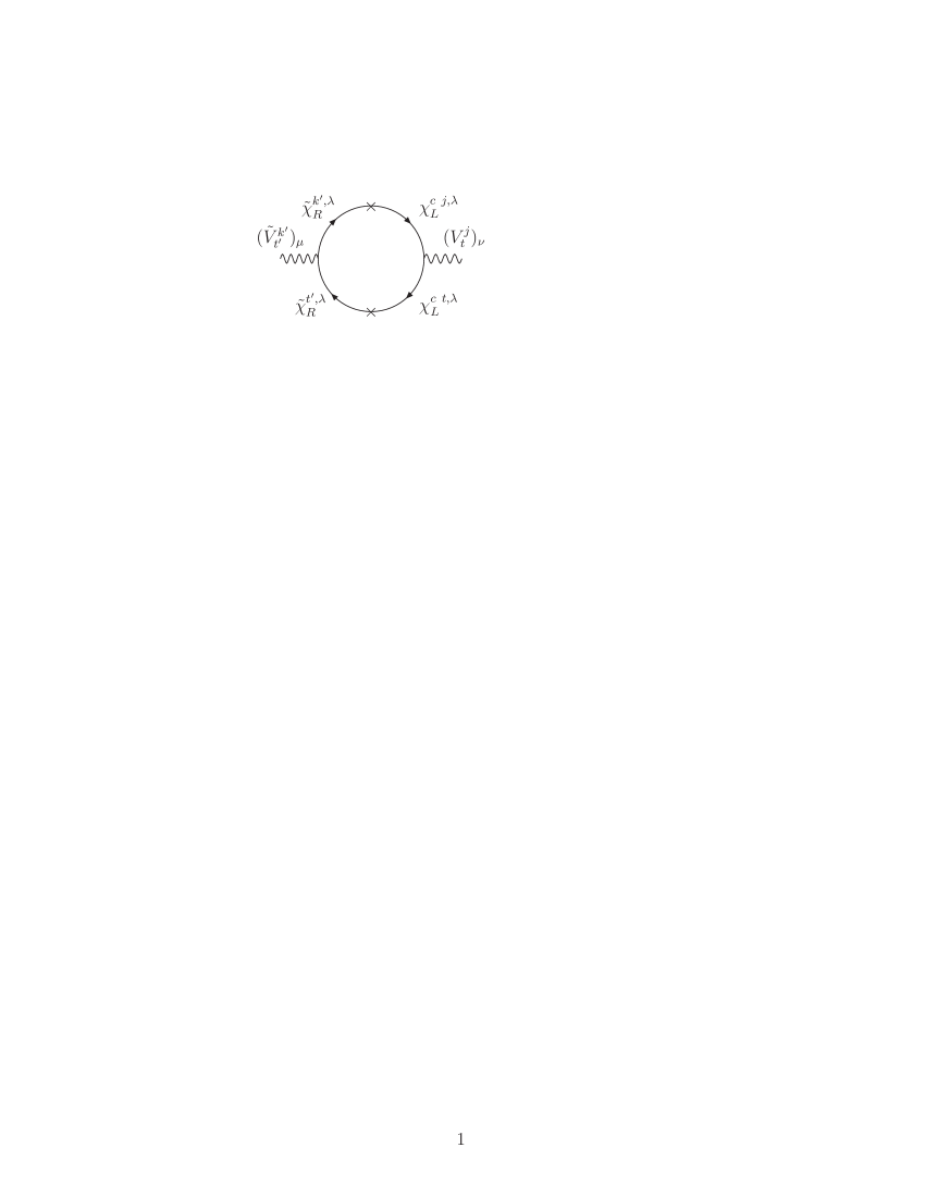
Figure 1: A graph contributing to the ETC gauge boson mixing $\tilde{V}^{k^{\prime}}_{t^{\prime}}\leftrightarrow V^{j}_{t}$, where $j,k^{\prime}\in\{1,2,3\}$ are generational indices and $t,t^{\prime}\in\{4,5\}$ connect with technicolor indices in SU(2)_TC, the diagonal subgroup of ${\rm SU}(2)_{ETC}\times{\rm SU}(2)^{\prime}_{ETC}$.

III.6 Quark and Lepton Masses

The effective theory describing the physics at energies $E<\Lambda_{TC}$, obtained by integrating out the ETC and TC gauge bosons and all of the heavy fermions, contains the mass matrix of the up-type quarks,

$${\cal L}_{u}=-\bar{u}_{j,L}M^{(u)}_{jk}u^{k}_{R}+h.c.,$$ (126)

and the corresponding mass matrix of the down-type quarks,

$${\cal L}_{d}=-\bar{d}_{j,L}M^{(d)}_{jk^{\prime}}d^{k^{\prime}}_{R}+h.c.,$$ (127)

with $j,k^{\prime}\in\{1,2,3\}$. For the present model, of L1 type, the mass matrix for the charged leptons is

$${\cal L}_{e}=-\bar{e}_{j^{\prime},L}M^{(e)}_{j^{\prime}k}e^{k}_{R}+h.c.,$$ (128)

with $j^{\prime},k\in\{1,2,3\}$. An analogous operator, with obvious interchange of primed indices, applies for a model of type L2.

Figure 2: A graph generating $\bar{u}_{j,L}M^{(u)}_{jk}u^{k}_{R}$ where $j,k\in\{1,2,3\}$ are generational indices and $t\in\{4,5\}$ are technicolor indices. The $V^{j}_{t}$ are SU(5)_ETC vector bosons.

The elements of the up-type quark mass matrix arise from the diagram in Fig. 2. The diagonal elements of this matrix are

$$M^{(u)}_{jj}\simeq\frac{\kappa\eta\Lambda_{TC}^{3}}{\Lambda_{j}^{2}}$$ (129)

where $\kappa\sim O(10)$ is a numerical prefactor from the integration (see, e.g., ckm ) and $\eta$ is a walking factor

$$\eta=\exp[\int_{\Lambda_{TC}}^{\Lambda_{w}}(d\mu/\mu)\gamma(\alpha(\mu))]$$ (130)

where the technicolor theory has walking behavior between $\Lambda_{TC}$ and a scale denoted $\Lambda_{w}$. With the anomalous dimension $\gamma\simeq 1$ as in a walking theory, this factor is then $\eta\simeq\Lambda_{w}/\Lambda_{TC}$. In the current class of theories, it is plausible that there could be walking up to the scale $\Lambda_{MC}$, so that $\eta\simeq\Lambda_{MC}/\Lambda_{TC}$. For the third-generation standard-model fermions, the entries $M^{(f)}_{33}$ should give reasonable estimates of the corresponding masses of $u^{3}\equiv t$, $d^{3}\equiv b$, and $e^{3}\equiv\tau$ which are not changed significantly by off-diagonal entries. In particular, for the top quark, assuming the above value of $\eta$ and using the value $\Lambda_{3}\simeq 3$ TeV, one obtains a value of $M^{(u)}_{33}$ and hence $m_{t}$ that is acceptably close to the experimental pole mass $m_{t}\simeq 175$ GeV. For $m_{t}$, the difference between this pole mass and the running mass evaluated at 175 GeV is negligible; for the other quarks, we use the running masses evaluated at the scale $\mu_{t}=175$ GeV. In view of the substantial uncertainties in the dynamically generated standard-model fermion masses due to the strong-coupling nature of the TC and ETC theories, we consider an estimate for a fermion mass to be acceptable if it is within a factor of 2-3 of the measured mass. If the contributions of off-diagonal element in $M^{(u)}$ are sufficiently small, then the diagonal element $M^{(f)}_{22}$ is dominant in determining the mass of the corresponding second-generation fermions $u^{2}\equiv c$. Assuming that this is the case, the value of $\Lambda_{2}\simeq 45$ TeV, which is consistent with the renormalization group equations for the SU(4)_ETC theory, yields an acceptable result for $m_{c}$, i.e., $m_{c}(\mu_{t})\simeq 0.6$ GeV, corresponding to the pole mass $m_{c}=1.3$ GeV. These values are listed in Table 1 together with other scales in the model. The property $m_{u}<m_{d}$ for first-generation quarks, which is the opposite of the pattern $m_{c}\gg m_{s}$, $m_{t}\gg m_{b}$ of the second and third generations, requires that some off-diagonal elements of $M^{(u)}$ and $M^{(d)}$ play an important role in determining the first-generation quark masses.

Table 1: Summary table of ETC and ETC^′ breaking scales and other strong-coupling scales, in units of TeV, in the model. In the third column we list a physical quantity or constraint(s) that are highly correlated with the numerical value of the given scale. In the lines for $\Lambda_{s}$ and $\Lambda_{s}^{\prime}$, $f=u,d,e$ refers to up- and down-quark quarks and charged leptons. In the line for $\Lambda_{MC}$, the notation $\{m_{d}\}$,  $\{m_{e}\}$ indicates that $\Lambda_{MC}$ affects the values of all of the down-type quarks and charged leptons. See text for detailed discussion.

scale	value	comments
$\Lambda_{1}$	$\simeq 10^{3}$	FCNC constraints
$\Lambda_{2}$	$\simeq 45$	$m_{c}$ value
$\Lambda_{3}$	$\simeq 3$	$m_{t}$ value
$\Lambda_{1}^{\prime}$	$\simeq 10^{3}$	FCNC constraints
$\Lambda_{2}^{\prime}$	$\simeq 15$	ETC hierarchy
$\Lambda_{3}^{\prime}$	$\simeq 15$	$m_{b}$ value
$\Lambda_{s}$	$\simeq 3$	$M^{(f)}$, off-diag.
$\Lambda_{s}^{\prime}$	$\simeq 3$	$M^{(f)}$, off-diag.
$\Lambda_{MC}$	$\simeq 2$	$\{m_{d}\}$,  $\{m_{e}\}$
$\Lambda_{TC}$	$\simeq 0.25$	$m_{W}$,  $m_{Z}$

The off-diagonal entries $M^{(u)}_{jk}$, $j\neq k$, arise via diagrams involving ETC vector boson mixing of the form $V^{k}_{t}\to V^{j}_{t}$. This mixing is indicated by the cross on the ETC vector boson propagator in Fig. 2, where it is understood that since the ETC and TC couplings are strong, further gauge boson exchanges not suppressed by large propagators are implicitly included.

$$M^{(u)}_{jk}\simeq\frac{\kappa\eta\ ({}^{j}_{t}\Pi^{k}_{t})\Lambda_{TC}^{3}}{\Lambda_{j}^{2}\Lambda_{k}^{2}}$$ (131)

where ${}^{j}_{t}\Pi^{k}_{t}$ denotes the relevant nondiagonal ETC propagator insertion that produce the transition $V^{k}_{t}\to V^{j}_{t}$. Additional virtual SU(5)_ETC exchanges not overly suppressed by large mass scales are understood to be included, since the corresponding gauge couplings are large.

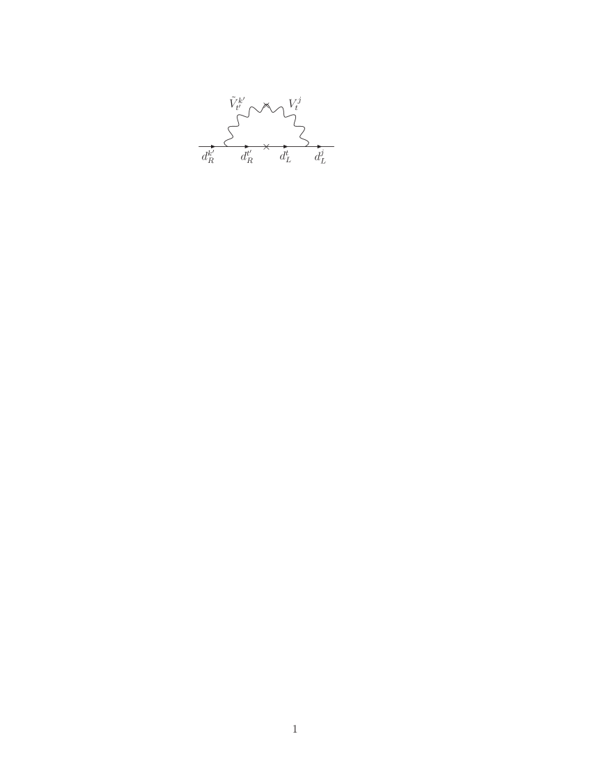
Figure 3: A graph generating the mass matrix for charge $q=-1/3$ quarks, $\bar{d}_{j,L}M^{(d)}_{jk^{\prime}}d^{k^{\prime}}_{R}$, where $j,k^{\prime}\in\{1,2,3\}$ are generational indices and $t,t^{\prime}\in\{4,5\}$ connect with technicolor indices in SU(2)_TC, the diagonal subgroup of ${\rm SU}(2)_{ETC}\times{\rm SU}(2)^{\prime}_{ETC}$. The $V^{j}_{t}$ and $\tilde{V}^{k^{\prime}}_{t^{\prime}}$ are SU(5)_ETC and SU(5)${}^{\prime}_{ETC}$ vector bosons; since the corresponding gauge couplings are strong, this graph is understood to represent also additional exchanges of these gauge bosons, insofar as they are not suppressed by large mass scales.

The down-quark and charged lepton masses are suppressed, since all elements of the mass matrices $M^{(d)}_{jk^{\prime}}$ and $M^{(e)}_{j^{\prime}k}$ require the $V-\tilde{V}$ mixing. The elements of the matrix $M^{(d)}$ arise from the graph in Fig. 3. We have

$$M^{(d)}_{jk^{\prime}}\simeq\frac{\kappa\eta\ ({}^{j}_{t}\Pi^{k^{\prime}}_{t^{\prime}})\Lambda_{TC}^{3}}{\Lambda_{j}^{2}\Lambda_{k}^{\prime 2}}$$ (132)

where ${}^{j}_{t}\Pi^{k^{\prime}}_{t^{\prime}}$ denotes the relevant nondiagonal ETC vector bosons propagator insertions and exchanges that produce the transition $\tilde{V}^{k^{\prime}}_{t^{\prime}}\to V^{j}_{t}$. Again, additional SU(5)_ETC and SU(5)${}^{\prime}_{ETC}$ exchanges not overly suppressed by large mass scales are understood to be included, since the corresponding gauge couplings are large. Since the metacolor condensate (95) occurs at the scale $\Lambda_{MC}$, it follows that the dynamical masses for the metacolor fermions are soft for higher momentum scales. Performing the loop integral in Fig. 1, one thus finds that ${}^{j}_{t}\Pi^{j^{\prime}}_{t^{\prime}}\propto\Lambda_{MC}^{2}$ for $j=j^{\prime}$ (with smaller values for ${}^{j}_{t}\Pi^{k^{\prime}}_{t^{\prime}}$ for $j\neq k^{\prime}$). The largest eigenvalues of $M^{(u)}$ and $M^{(d)}$, i.e., the masses of $m_{t}$ and $m_{b}$, are determined by the respective elements $M^{(u)}_{33}$ and $M^{(d)}_{33}$. From eqs. (129) and (132), one then has the relation

$$\frac{m_{b}}{m_{t}}\simeq\left(\frac{\Lambda_{MC}}{\Lambda_{3}^{\prime}}\right)^{2}$$ (133)

since the factor of $1/\Lambda_{3}^{2}$ cancels in this ratio. Using the pole mass $m_{b}\simeq 4.3$ GeV or equivalently the running mass $m_{b}(\mu_{t})\simeq 3.0$ GeV, with $m_{t}\simeq 175$ GeV as above, eq. (133) yields the ratio $\Lambda_{3}^{\prime}/\Lambda_{MC}\simeq 7.6$. With the illustrative value $\Lambda_{MC}\simeq 2$ TeV, this can be achieved with $\Lambda_{3}^{\prime}\simeq 15$ TeV. Because of the strong-coupling nature of the physics involved here, these are only rough estimates, but they demonstrate that the model can achieve the requisite $t-b$ mass splitting.

However, the model encounters difficulty in trying to account for the masses of the standard-model fermions of the lower two generations. To see this, we first consider the situation in the approximation where one neglects the off-diagonal terms in the mass matrices. Then the model would yield the generalization of eq. (133), viz.,

$$\frac{m_{d_{j}}}{m_{u_{j}}}=\bigg{(}\frac{\Lambda_{MC}}{\Lambda_{j}^{\prime}}\bigg{)}^{2}$$ (134)

for generation $j$. Taking ratios for $j=2$ and $j=3$, this would imply the double ratio relation

$$\frac{(m_{s}/m_{c})}{(m_{b}/m_{t})}=\left(\frac{\Lambda_{3}^{\prime}}{\Lambda_{2}^{\prime}}\right)^{2}$$ (135)

(where all of the masses are evaluated at a common scale, taken here to be $\mu_{t}$). But because $m_{s}/m_{c}>m_{b}/m_{t}$ (the values being roughly 1/10 and 1/60, respectively), this would require that $\Lambda_{3}^{\prime}>\Lambda_{2}^{\prime}$, which is impossible, since the sequential breaking ${\rm SU}(4)^{\prime}_{ETC}\to{\rm SU}(3)^{\prime}_{ETC}$ guarantees that $\tilde{\Lambda}_{2}\geq\tilde{\Lambda}_{3}$. This problem would be mitigated as much as possible if $\Lambda_{2}^{\prime}\simeq\Lambda_{3}^{\prime}$, i.e. the sequential breaking of SU(4)${}^{\prime}_{ETC}$ to SU(3)${}^{\prime}_{ETC}$ and thence to SU(2)${}^{\prime}_{ETC}$ occurs at comparable scales (see Table 1).

There is also a problem with the ratios of down-quark masses of different generations. With the same simplification of neglecting off-diagonal elements in the mass matrix $M^{(d)}$, one has

$$\frac{m_{d_{j}}}{m_{d_{k}}}=\bigg{(}\frac{\Lambda_{k}\Lambda_{k}^{\prime}}{\Lambda_{j}\Lambda_{j}^{\prime}}\bigg{)}^{2}\ .$$ (136)

This yields ratios for $m_{s}/m_{b}$ and $m_{d}/m_{s}$ that are too small to fit experimental values. One is thus motivated to consider the full down-quark mass matrix in order to assess whether this improves the predictions for the ratios (136). We define the ratios

$$r_{jk}\equiv\left(\frac{\Lambda_{j}}{\Lambda_{k}}\right)^{2}\ ,\quad r^{\prime}_{jk}\equiv\left(\frac{\Lambda_{j}^{\prime}}{\Lambda_{k}^{\prime}}\right)^{2}\ .$$ (137)

We can then write eq. (132) equivalently as

$$M^{(d)}\simeq m_{b}\left(\begin{array}[]{ccc}r_{31}r^{\prime}_{31}&r_{31}r^{\prime}_{32}&r_{31}\\ r_{32}r^{\prime}_{31}&r_{32}r^{\prime}_{32}&r_{32}\\ r^{\prime}_{31}&r^{\prime}_{32}&1\end{array}\right)\ .$$ (138)

Diagonalizing this matrix, one finds that the presence of the off-diagonal elements does not change the mass eigenvalues sufficiently from the diagonal-matrix case, so that the masses for the first two generations, $m_{d}$ and $m_{s}$, are still too small. If these off-diagonal elements were larger than our estimates above, this problem might be ameliorated somewhat.

Figure 4: A graph generating the mass matrix for charged leptons, $\bar{e}_{j^{\prime},L}M^{(e)}_{j^{\prime}k}e^{k}_{R}$, where $j^{\prime},k\in\{1,2,3\}$ are generational indices and $t,t^{\prime}\in\{4,5\}$ connect with technicolor indices in SU(2)_TC, the diagonal subgroup of ${\rm SU}(2)_{ETC}\times{\rm SU}(2)^{\prime}_{ETC}$. Notation is as in Fig. 3.

In this model of type L1, the elements of the charged lepton mass matrix in eq. (128) are generated via the graph shown in Fig. 4, leading to the result

$$M^{(e)}_{j^{\prime}k}\simeq\frac{\kappa\eta\,({}^{j^{\prime}}_{t}\Pi^{k}_{t})\Lambda_{TC}^{3}}{\Lambda_{j}^{\prime 2}\Lambda_{k}^{2}}\ .$$ (139)

The model succeeds in producing the desired $t-\tau$ mass splitting, but, as was the case with $M^{(d)}$ and for the same reasons, the values of $m_{e}$ and $m_{\mu}$ are too small. For comparison, we note that a similar problem with overly small $m_{d,s}$ and $m_{e,\mu}$ masses was encountered in the model that we studied earlier in Refs. ckm ; kt which used relatively conjugate representations for the left- and right-handed chiral components of the down-quarks and charged leptons to obtain intragenerational mass splittings.

In addition to the suppression of the $Q=-1/3$ quark mass relative to the $Q=2/3$ quark mass in the upper two generations, a viable model should also incorporate a mechanism for suppressing the charged lepton mass relative to the $Q=2/3$ and $Q=-1/3$ quark masses in each generation. In a theory such as the present one with walking, the technicolor coupling varies slowly with energy over an extended interval and is only slightly less than the critical value for condensate formation. Therefore, small perturbations that would normally be of negligible importance can become significant. In particular, the attractive QCD interaction can naturally expedite techniquark condensation, relative to technilepton condensation (in a one-family model), so that the former occurs at a higher energy scale than the latter, giving rise to the inequality $\Sigma_{Q}>\Sigma_{L}$ for the resultant dynamical techniquark and technilepton masses, and consequently to an increase of the quark masses, relative to the charged lepton masses, in each generation qcdcor ; met1 . However, this, by itself, does not split the masses of the charge 2/3 quarks from those of the charge $-1/3$ quarks. For that purpose, one could invoke the U(1)_Y hypercharge gauge interactions, which are weaker.

IV Some Further Phenomenological Topics

IV.1 Flavor-Changing Neutral Current Processes

The present models can satisfy constraints from flavor-changing neutral current processes. The basic observation here is the generalization of the point made in Ref. ckm to the case of two ETC groups: because both of the ETC gauge interactions act in a vectorial, rather than chiral, manner on the standard-model quarks, processes such as $\bar{K}^{0}\leftrightarrow K^{0}$, $\bar{D}^{0}\leftrightarrow D^{0}$, and $\bar{B}^{0}_{q}\to\bar{B}^{0}_{q}$ with $q=d,s$ are suppressed. For example, to take the transition among these that imposes the most severe constraint, namely the one with neutral kaons, in the $\bar{K}^{0}\to K^{0}$ transition, an initial $s_{L}\bar{d}_{L}$ produces a $V^{2}_{1}$ ETC gauge boson, but this cannot directly yield a $d_{L}\bar{s}_{L}$ in the final-state $K^{0}$; the latter is produced by a $V^{1}_{2}$. This requires ETC gauge boson mixing of the form $V^{2}_{1}\to V^{1}_{2}$. In the present models, as in the simpler vectorial model with a single ETC group studied in Ref. ckm ; kt , this mixing introduces a suppression by a factor $\simeq(\Lambda_{3}/\Lambda_{1})^{2}$, resulting in an ETC contribution to $\bar{K}^{0}-K^{0}$ mixing and hence to $\Delta m_{K}$ of order $\Lambda_{3}^{2}\Lambda_{QCD}^{3}/\Lambda_{1}^{4}$, where $\Delta m_{K}=m_{K_{L}}-m_{K_{S}}=(0.7\times 10^{-14})m_{K^{0}}$, and we ignore factors of $1/(4\pi^{2})$ in view of the strong-coupling nature of the calculation. Requiring that the ETC contribution be small compared with the experimentally measured value of $\Delta m_{K}$ implies that the ratio $\Lambda_{3}\Lambda_{QCD}/\Lambda_{1}^{2}\ll 10^{-7}$. This constraint is satisfied, for example, by the illustrative values of $\Lambda_{1}\simeq 10^{3}$ TeV and $\Lambda_{3}=3$ TeV used here, which give $\Lambda_{3}\Lambda_{QCD}/\Lambda_{1}^{2}\simeq 0.6\times 10^{-9}$. Similarly, in the same $\bar{K}^{0}\to K^{0}$ transition, an initial $s_{R}\bar{d}_{R}$ produces a $\tilde{V}^{2}_{1}$ ETC gauge boson, but this cannot directly yield a $d_{R}\bar{s}_{R}$ in the final-state $K^{0}$; the latter is produced by a $\tilde{V}^{1}_{2}$. This requires ETC gauge boson mixing of the form $\tilde{V}^{2}_{1}\to\tilde{V}^{1}_{2}$, which causes a suppression by a factor $\simeq(\Lambda_{3}^{\prime}/\Lambda_{1}^{\prime})^{2}$. By the same reasoning as above, we require that the ratio $\Lambda_{3}^{\prime}\Lambda_{QCD}/(\Lambda_{1}^{\prime})^{2}\ll 10^{-7}$. This constraint is satisfied for the values of these parameters used here, which give a value of $\simeq 3\times 10^{-9}$ for this ratio. Analogous remarks apply for the contributions via $s_{L}\bar{d}_{L}\to V^{2}_{1}\to\tilde{V}^{1}_{2}\to d_{R}\bar{s}_{R}$ and $s_{R}\bar{d}_{R}\to\tilde{V}^{2}_{1}\to V^{1}_{2}\to d_{L}\bar{s}_{L}$.

The same type of suppression occurs for other neutral pseudoscalar meson mixings such as $D\leftrightarrow\bar{D}$, $B_{d}\leftrightarrow\bar{B}_{d}$, and $B_{s}\leftrightarrow\bar{B}_{s}$. The upper limit on the decay $K^{+}\to\pi^{+}\mu^{+}e^{-}$ and hence on the elementary process $\bar{s}\to\bar{d}\mu^{+}e^{-}$, which is mediated by $V^{1}_{2}$ and $\tilde{V}^{1}_{2}$, is also satisfied with the values of $\Lambda_{1}$ and $\Lambda_{1}^{\prime}$ that we use. Similar consistency checks can be carried out for other processes and quantities due to dimension-5 and dimension-6 operators, as we have analyzed these in earlier works ckm -qdml .

IV.2 Neutrino Masses

In Ref. nt a mechanism was presented for producing light neutrino masses in an ETC theory. This was studied further in Refs. lrs ; ckm . Here we remark on how this mechanism can be implemented in the current models containing two ETC gauge groups. For this purpose, we recall that even in an ETC theory with only one ETC group, below the highest scale, $\Lambda_{1}$, of ETC breaking, there are actually two plausible patterns of breaking. These were labelled $G_{a}$ and $G_{b}$ in Ref. nt , and, in modified form, sequences S1 and S2 in Refs. ckm ; kt . In the discussion above we have concentrated on the two-ETC group generalization of sequence S1. For considerations of neutrino masses, sequence S2 is also of interest. One would thus be led to consider a generalization of this sequence to the case of two ETC groups relevant to the present models.

IV.3 Remarks on a Model with a Minimal Technifermion Sector

Two continuing concerns that one has with ETC models that contain a full standard-model family of technifermions are the substantial contribution to the electroweak parameter $S$ and the presence of many pseudo-Nambu-Goldstone bosons (PNGB’s), whose masses must be elevated (e.g., by walking enhancement) to lie above experimental lower bounds. These concerns motivate consideration of ETC models which use the minimum set of electroweak-nonsinglet technifermions, comprising (for a given TC index) a single left-handed SU(2)_L doublet and the corresponding two right-handed fields. We briefly comment here on how one might construct a model of this type with two ETC groups.

We denote the technicolor contribution to $S$ as $(\Delta S)^{(TC)}$. In general, the $S$ parameter pt measures heavy-particle contributions to the $Z$ self-energy via the term $4s_{W}^{2}c_{W}^{2}\alpha^{-1}_{em}(m_{Z})[\Pi^{(NP)}_{ZZ}(m_{Z}^{2})-\Pi^{(NP)}_{ZZ}(0)]/m_{Z}^{2}$, where $s_{W}^{2}=1-c_{W}^{2}=\sin^{2}\theta_{W}$, evaluated at $m_{Z}$ (see pdg for details). Since technifermions are strongly interacting on the scale $m_{Z}$ used in the definition of $S$, one cannot reliably apply perturbation theory to calculate $(\Delta S)^{(TC)}$ scalc1 ; scalc2 ; at most, it provides a rough guide, namely, $(\Delta S)^{(TC)}_{pert.}=N_{D}/(6\pi)$, where $N_{D}$ denotes the total number of new technifermion SU(2)_L doublets (counting technicolors). As is well known, for a one-family technicolor with technifermions transforming according to the fundamental representation of SU($N_{TC}$), $N_{D}=N_{TC}(N_{c}+1)=8$, so that $(\Delta S)^{(TC)}_{pert.}=4/(3\pi)\simeq 0.4$, which is larger than the experimentally preferred region.

Now consider a TC/ETC model with a minimal electroweak-nonsinglet technifermion sector. For general $N_{TC}$, we again take the technifermions to transform according to the fundamental representation of SU($N_{TC}$). The transformation properties of the SM-nonsinglet technifermions under ${\rm SU}(N_{TC})\times G_{SM}$ are given by

$$F^{p,t}_{L}={F^{1,t}_{L}\choose F^{2,t}_{L}}\ :\ (N_{TC},1,2)_{0,L},$$ (140)

(141)

$$F^{t\ (\pm 1/2)}_{R}\ :\ \ (N_{TC},1,1)_{\pm 1,R},$$ (142)

where $p=1,2$ and $t$ are the SU(2)_L and SU($N_{TC}$) indices, the superscripts in parentheses indicate electric charge, and the subscripts are hypercharge and chirality. (The charges on $F^{p,t}_{L}$ are obvious and hence are suppressed in the notation.) For this model, $(\Delta S)^{(TC)}_{pert.}=N_{TC}/(6\pi)$. Hence, for $N_{TC}=2$, $(\Delta S)^{(TC)}_{pert.}=1/(3\pi)\simeq 0.1$, which is sufficiently small to agree with experimental constraints. Although one-doublet technicolor models, as such, do not have walking, one can add SM-singlet, TC-nonsinglet fermions so as to produce walking ts . Another advantage of a one-doublet TC model is that all of the three Nambu-Goldstone bosons (NGB’s) that arise due to the formation of technicondensates are absorbed to make the $W^{\pm}$ and $Z$ massive so that there are no problems with unwanted PNGB’s.

In this model, as the energy scale descends to $\Lambda_{TC}$, the TC interaction naturally leads to the formation of the technifermion condensates

$$\langle\bar{F}_{1,t,L}F^{(1/2),t}_{R}\rangle\ ,\quad\langle\bar{F}_{2,t,L}F^{(-1/2),t}_{R}\rangle$$ (143)

breaking electroweak symmetry in the desired manner. This channel has $\Delta C_{2}=(N_{TC}^{2}-1)/N_{TC}$, i.e., 3/2 for $N_{TC}=2$. We note that for $N_{TC}=2$ an equally attractive channel would involve the condensate

$$\langle\epsilon_{pq}\epsilon_{st}F^{ps\ T}_{L}CF^{qt}_{L}\rangle$$ (144)

$$= \langle\epsilon_{st}(F^{1s\ T}_{L}CF^{2t}_{L}-F^{2s\ T}_{L}CF^{1t}_{L})\rangle$$ (146)

where $p,q$ and $s,t$ are SU(2)_L and SU(2)_TC indices, respectively. One would not want (146) to be the only technifermion condensate to occur, since it is invariant under the entire group $G$ in eq. (6) and thus, in particular, does not break the electroweak gauge symmetry. It would be worthwhile in future work to investigate how this type of TC model with a minimal electroweak-nonsinglet technifermion sector could be embedded in a larger theory with two ETC gauge groups.

V Conclusions

In this paper we have formulated a class of extended technicolor models that can plausibly produce the observed mass splitting $m_{t}\gg m_{b}$ without excessive contributions to the $\rho$ parameter or to neutral flavor-changing processes. These models use two different chiral ETC groups met1 such that left- and right-handed components of charge 2/3 quarks transform under the same ETC group, while left- and right-handed components of charge $-1/3$ quarks and charged leptons transform under different ETC groups. The models suppress $m_{b}$ and $m_{\tau}$ relative to $m_{t}$, and $m_{s}$ and $m_{\mu}$ relative to $m_{c}$ because the masses of the $Q=-1/3$ quarks and charged leptons require mixing between the two ETC groups, while the masses of the $Q=2/3$ quarks do not. We have constructed and analyzed in detail one explicit model of this type. Clearly, since the relative sizes of the quark masses in the first generation are opposite to the order for the higher two generations, i.e., $m_{d}>m_{u}$, the strategy used in these classes of models would not, by itself, be expected to account for this. However, it is also difficult to account for the absolute sizes of $m_{s}$ and $m_{d}$, and of $m_{\mu}$ and $m_{e}$; the suppression mechanism makes these smaller than the respective observed values. A similar problem was encountered in a model using relatively conjugate representations of a single ETC gauge group for left- and right-handed chiral components to obtain intragenerational mass splittings in Refs. ckm ; kt . Although the model is rather complicated, we believe that it is useful as explicit, moderately ultraviolet-complete realization of the strategy of using two different ETC groups to account for the splitting between $m_{t}$ and $m_{b}$.

References

• (1) S. Weinberg, Phys. Rev. D 19, 1277 (1979); L. Susskind, ibid. D 20, 2619 (1979); S. Weinberg, Phys. Rev. D 13, 974 (1976).
• (2) S. Dimopoulos, L. Susskind, Nucl. Phys. B155, 23, (1979); E. Eichten, K. Lane, Phys. Lett. B 90, 125 (1980).
• (3) K. Lane, hep-ph/0202255; C. Hill and E. Simmons, Phys. Rep. 381, 235 (2003); R. S. Chivukula, M. Narain, and J. Womersley, in Ref. pdg .
• (4) http://pdg.lbl.gov.
• (5) http://lepewwg.web.cern.ch/LEPEWWG/plots
• (6) B. Holdom, Phys. Lett. B 150, 301 (1985); K. Yamawaki, M. Bando, and K. Matumoto, Phys. Rev. Lett. 56, 1335 (1986); T. Appelquist, D. Karabali, and L. C. R. Wijewardhana, Phys. Rev. Lett. 57, 957 (1986); T. Appelquist and L.C.R. Wijewardhana, Phys. Rev. D 35, 774 (1987); Phys. Rev. D 36, 568 (1987).
• (7) T. Appelquist, J. Terning, and L. C. R. Wijewardhana, Phys. Rev. Lett. 77, 1214 (1996); Phys. Rev. T. Appelquist, A. Ratnaweera, J. Terning, and L. C. R. Wijewardhana, Phys. Rev. D 58, 105017 (1998).
• (8) T. Appelquist, N. Evans, and S. Selipsky, Phys. Lett. B 374, 145 (1996).
• (9) T. Appelquist, J. Terning, Phys. Rev. D 50, 2116 (1994).
• (10) S. Glashow and S. Weinberg, Phys. Rev. D 15, 1958 (1977).
• (11) P. Sikivie, L. Susskind, M. Voloshin and V. Zakharov, Nucl. Phys. B 173, 189 (1980).
• (12) J. Terning, Phys. Lett. B 344, 279 (1995).
• (13) T. Appelquist, M. Piai and R. Shrock, Phys.Β Rev.Β D 69, 015002 (2004)
• (14) T. Appelquist, N. Christensen, M. Piai and R. Shrock, Phys. Rev. D 70, 093010 (2004).
• (15) T. Appelquist, M. Piai and R. Shrock, Phys.Β Lett.Β B 593, 175 (2004)
• (16) T. Appelquist, M. Piai and R. Shrock, Phys.Β Lett.Β B 595, 442 (2004)
• (17) M. Peskin and T. Takeuchi, Phys. Rev. D 46, 381 (1992).
• (18) M. Golden and L. Randall, Nucl. Phys. B 361, 3 (1991); R. Johnson, B.-L. Young, and D. McKay, Phys. Rev. D 43, R17 (1991); R. Cahn and M. Suzuki, Phys. Rev. D 44, 3641 (1991).
• (19) T. Appelquist and G. Triantaphyllou, Phys. Lett. B 278, 345 (1992); R. Sundrum and S. Hsu, Nucl. Phys. B 391, 127 (1993); T. Appelquist and J. Terning, Phys. Lett. B315, 139 (1993); T. Appelquist, J. Terning, L.C.R. Wijewardhana, Phys. Rev. Lett. 79, 2767 (1997). T. Appelquist and F. Sannino, Phys. Rev. D 59, 067702 (1999); S. Ignjatovic, L. C. R. Wijewardhana, and T. Takeuchi, ibid. D 61, 056006 (2000); M. Harada, M. Kurachi, and K. Yamawaki, in Proc. Dynamical Symmetry Breaking Workshop (Dec. 2004), p. 125; M. Harada, M. Kurachi, and K. Yamawaki, hep-ph/0509193 (we thank Dr. Kurachi for useful discussions on this work); N. Christensen and R. Shrock, Phys. Rev. Lett. 94, 241801 (2005).
• (20) Some recent works on models to minimize TC contributions to $S$ include Refs. sann ; ts .
• (21) D. Hong, S. Hsu, and F. Sannino, Phys. Lett. B 597, 89 (2004).
• (22) N. Christensen and R. Shrock, Phys. Lett. B 632, 92 (2006).
• (23) T. Appelquist and R. Shrock, Phys. Lett. B548, 204 (2002).
• (24) T. Appelquist and R. Shrock, Phys. Rev. Lett. 90, 201801 (2003).
• (25) The reason that it is necessary to use two different hypercolor groups is that if one were to try to use just one, it would not be asymptotically free, and hence the HC interaction would not increase as the energy scale decreases. Consequently, this HC group would not fulfill its job of helping to produce various symmetry-breaking bilinear fermion condensates.
• (26) An alternative is to avoid a metacolor group and instead have the communication between the ETC and ETCβ€² groups carried out by one or more fermions that transform as nonsinglet(s) under both the ETC and ETCβ€² groups; this will be discussed elsewhere with T. Appelquist, Y. Bai, and M. Piai.
• (27) Our notation for the beta function of a gauge group $G_{j}$ is indicated below, where $\alpha_{j}=g_{j}^{2}/(4\pi)$,
$$\beta_{j}=\frac{d\alpha_{j}}{dt}=-\frac{\alpha_{j}^{2}}{2\pi}\left(b_{0}^{(j)}+\frac{b_{1}^{(j)}}{4\pi}\alpha_{j}+O(\alpha_{j}^{2})\right)$$
and $t=\ln\mu$ with $\mu$ being the momentum scale.
• (28) S. Raby, S. Dimopoulos, and L. Susskind, Nucl. Phys. B 169, 373 (1980).
• (29) In the approximation of a single-gauge-boson exchange, the critical coupling for chiral fermions transforming according to the representations $R_{1}$ and $R_{2}$ of a gauge group $G$ to form a condensate transforming as $R_{cond.}$ in an SU($N$) gauge theory is given by the condition $\alpha\geq\alpha_{cr}$, where $\alpha_{cr}\simeq 2\pi/(3\Delta C_{2})$, $\Delta C_{2}=[C_{2}(R_{1})+C_{2}(R_{2})-C_{2}(R_{c})]$, and $C_{2}(R)$ is the quadratic Casimir invariant casimir .
• (30) Our notation for the Casimir invariants $C_{2}(R)$ and $T(R)$ of the representation $R$ is given by ${\cal D}_{R}(T_{a})^{i}_{j}{\cal D}_{R}(T_{a})^{j}_{k}=C_{2}(R)\delta^{i}_{k}$ and $({\cal D}_{\cal R}(T_{a}))^{i}_{j}\ ({\cal D}_{\cal R}(T_{b}))^{j}_{i}=T({\cal R})\delta_{ab}$, where $\{a,b\}$ and $\{i,j,k\}$ denote group and representation indices and sums over repeated indices are understood.
• (31) For completeness, we note that there are other condensation channels with the same value of $\Delta C_{2}=24/5$, such as $(5,1;1,1,1;3,2)_{1/3,L}\times(\bar{5},1;1,1,1;\bar{3},1)_{-4/3,L}\to(1,1;1,1,1;1,2)_{-1}$ with condensate $\langle\bar{Q}_{a,j,L}u^{a,j}_{R}\rangle$ and $(5,1;1,1,1;1,1)_{0,R}\times(\bar{5},1;1,1,2;1,1)_{0,R}\to(1,1;1,1,2;1,1)_{0}$ with condensate $\langle{\cal N}^{j\ T}_{R}C\chi_{j,\lambda,R}\rangle$. These are both undesired; the former would break SU(2)L at too high a scale, and the latter would break SU(2)MC. Our scenario, in which the condensation (45) occurs, and the above two condensations do not occur, at this scale, is consistent with GMAC arguments, within the uncertainties concerning the properties of strongly coupled field theories.
• (32) A possible mechanism for suppressing a common dynamical technilepton mass $\Sigma_{N}\simeq\Sigma_{E}$ relative to a common techniquark mass $\Sigma_{U}\simeq\Sigma_{D}$ is briefly discussed later in the text. Since this preserves custodial symmetry, it does not directly contribute to the TC correction to $\rho$.
• (33) M. Veltman, Nucl. Phys. B 123, 89 (1977); Acta Phys. Pol. B 8, 475 (1977). Note that $f_{\rho}$ has the properties $f_{\rho}(x,y)=f_{\rho}(y,x)$, $f_{\rho}(x,x)=0$, and, for the physical case $x,y\geq 0$, $f_{\rho}(x,y)\geq 0$.
• (34) B. Holdom, Phys. Rev. Lett. 60, 1233 (1988); T. Appelquist and O. Shapira, Phys. Lett. B 249, 83 (1990).