CP, T and CPT analyses in EPR-correlated $B^{0}\bar{B^{0}}$ decays
PhD Thesis
author Ezequiel Álvarez
director José Bernabéu Alberola

A Carla, mi raison d’être

JOSÉ BERNABÉU ALBEROLA, Catedrático de Física Teórica de la Universidad de Valencia,

CERTIFICA:      Que la presente memoria ”CP, T AND CPT ANALYSES IN EPR-CORRELATED $B^{0}\bar{B^{0}}$ DECAYS” ha sido realizada bajo su dirección en el Departamento de Física Teórica de la Universidad de Valencia por el Licenciado D. EZEQUIEL ÁLVAREZ y constituye su Tesis Doctoral. Y para que así conste, presenta la referida memoria en Burjassot, a 1 de marzo de 2006
Firmado: José Bernabéu Alberola

Abstract

In this work we study the T, CP and CPT symmetries in the B-meson system. Our analysis and results are addressed to the case of correlated mesons in the B-factories.

In the first set of theory and results we investigate the consequences of these discrete symmetries in the B-mixing and interference between mixing and decay. With the help of the CP-tag we compute all possible intensities and asymmetries which concern flavour-specific and CP Golden Plate decays. Our proposed observables are a new self-consistency check for the Standard Model, as well as a new exploration for the traces of the discrete symmetries in the B-system.

In the second set of results we study CPT violation in the initial state of the B-factories through the loss of indistinguishability of $B^{0}$ and $\bar{B^{0}}$. We show that, if the consequence of Bose statistic is relaxed, then the equal-sign dilepton events are considerably modified. We analyze the demise of flavour tagging and we also prove that the equal-sign charge asymmetry, $A_{sl}$, is an optimal observable where to look for this new CPT violation effect. The detailed study of this asymmetry allows us to predict different behaviours according to the possible values of the CPT violating parameter $\omega$. We conclude that the best observable where to find traces of this novel kind of CPT violation is the analysis of $A_{sl}$ at small $\Delta t$’s. We use existing data on $A_{sl}$ to put the first limits on $\omega$.

En este trabajo estudiamos las simetrías T, CP y CPT en el sistema de mesones B. Nuestros análisis y resultados están dirigidos para el caso de mesones correlacionados en las fábricas de mesones B.

En el primer conjunto de teoría y resultados investigamos las consecuencias de estas simetrías discretas en el mixing de B’s y en la interferencia entre mixing y decaimiento. Con la ayuda del rótulo por CP (CP-tag) calculamos todas las posibles intensidades y asimetrías que conciernen a sabor-específico y decaimiento CP Golden Plate. Nuestros observables propuestos son una nueva verificación de auto-consistencia para el Modelo Estándar, así como una nueva exploración para los rastros de las simetrías discretas en el sistema de mesones B.

En el segundo conjunto de resultados estudiamos violación de CPT en el estado inicial de las fábricas de B a través de la pérdida de indistinguibilidad de $B^{0}$ y $\bar{B^{0}}$. Mostramos que, si se relaja el requisito de estadística de Bose, entonces los eventos dileptónicos de igual signo son considerablemente modificados. Analizamos el ’fin’ del rótulo por sabor (demise of flavour-tag) y también probamos que la asimetría de carga de eventos del mismo-signo, $A_{sl}$, es un observable óptimo donde buscar esta nueva clase de violación de CPT. El estudio detallado de esta asimetría nos permite predecir diferentes comportamientos de acuerdo con los posibles valores del parámetro de violación de CPT, $\omega$. Concluimos que el mejor observable para hallar rastros de esta flamante clase de violación de CPT es el análisis de $A_{sl}$ a tiempos cortos. También usamos medidas existentes de $A_{sl}$ para poner los primeros límites en $\omega$.

Chapter 1 Introduction

1.1 General Introduction

Symmetry may be one of the most interesting and outstanding archetypes of mankind. From the earliest homo-sapiens-sapiens legacy’s art motivation, running by the Egyptians, Greek, Romans, Arabs and every-other Civilization, and until the present day, we can detect it and feel it in a considerable amount of creations or inventions of man’s mind. Its power is so strong that some times may even corrupt the line between archetype and instinct.

Archetype or instinct, symmetry has proven to be an essential tool for the development of science. From the very first days of Natural Philosophy, Pythagoras VIth century BC, symmetry has furnished insight into the laws of physics and the nature of the Cosmos. This insight has found always a constant evolution with the pass of time and the depth of knowledge, and it is worth to briefly point out some landmarks.

In the late XVIIth century I. Newton and G.W. Leibniz created the infinitesimal calculus and, in particular, the latter developed the analytic notation, which replaced geometry as the essential tool to study physical systems. At first sight this could have looked as a step backward in the art of taking profit of symmetries to understand physical systems, but in the following century J.-L. Lagrange and W. Hamilton proved this was not the case. They invented the Lagrangian formalism, in which all the symmetries of the system are explicitly incorporated and transformed into conservation laws, and hence improving considerably, with respect to geometry, the depth of the insight that symmetries can furnish in the physical theories and in the understanding of the Universe. Moreover, in this formalism many times the symmetries of the system itself can determine the Lagrangian, and therefore all the physical theory behind it. It is clear that all these achievements would not have been possible without a mathematical baggage which could, first define symmetry, and then incorporate it analytically into the theory: this was the invention of Group Theory, in the XVIIIth and XIXth century by the great mathematicians J.-L. Lagrange and E. Galois. At present day, symmetry is one of the chief concepts of modern physics and mathematics. The two outstanding theoretical development of the XXth century, Relativity and Quantum Theory, involve notions of symmetry in a fundamental and irreplaceable way. We should not be surprised if, in the future, the laws of Nature end up being written uniquely in terms of symmetry notions.

It is clear that the study and analysis of symmetries is essential for the understanding and development of physics. In their study, the first major division occurs between continuous and discrete symmetries. In this work we propose to study, within the frame of the B-meson system in particle physics, the discrete symmetries C, P, T and their relevant combinations CP, T, and CPT.

In particle physics, charge conjugation (C) is a mathematical operation that changes all the charge’s sign of a particle, for instance, changing the sign of the electrical charge. Charge conjugation implies that every charged particle has an oppositely charged antimatter counterpart, or antiparticle. The antiparticle of an electrically neutral particle may be identical to the particle, as in the case of the neutral pi meson, or it may be distinct, as with the anti-neutron due to baryon number. Parity (P), or space inversion, is the reflection in the origin of the space coordinates of a particle or particle system; i.e., the three space dimensions $x$, $y$, and $z$ become, respectively, $-x$, $-y$, and $-z$. Time reversal (T) is the mathematical operation of replacing the expression for time with its negative in formulas or equations so that all the motions are reversed. A resultant formula or equation that remains unchanged by this operation is said to be time-reversal invariant, which implies that the same laws of physics apply equally well in both situations. A motion picture of two billiard balls colliding, for instance, can be run forward or backward with no clue of which of both is the original sequence.

For years it was assumed that charge conjugation, parity and time reversal were exact symmetries of elementary processes, namely those involving electromagnetic, strong, and weak interactions. However, a series of discoveries from the mid-1950s caused physicists to alter significantly their assumptions about the invariance of C, P, and T. An apparent lack of the conservation of parity in the decay of charged K mesons into two or three pi mesons prompted C.N. Yang and T.-D. Lee to examine the experimental foundation of parity itself. In 1956 they showed that there was no evidence supporting parity invariance in weak interactions. Experiments conducted the next year by Madame C.-S. Wu verified decisively that parity was violated in the weak interaction beta decay. Moreover, they revealed that charge conjugation symmetry also was broken during this decay process. The discovery that the weak interaction conserves neither charge conjugation nor parity separately, however, led to a quantitative theory establishing combined CP as a symmetry of nature. Physicists reasoned that if CP were invariant, time reversal T would have to remain so as well due to the CPT theorem. But further experiments, carried out in 1964, demonstrated that the long-life electrically neutral K meson, which was thought to break down into three pi mesons, decayed a fraction of the time into only two such particles, thereby violating CP symmetry. CP violation implied nonconservation of T, provided that the long-held CPT theorem was valid. In this theorem, regarded as one of the basic principles of quantum field theory, charge conjugation, parity, and time reversal are applied together. As a combination, these symmetries constitute an exact symmetry of all types of fundamental interactions. In any case, experiments are testing this CPT invariance – which up to now it has not been seen to be violated.

CP and T-violation have important theoretical consequences. The violation of CP symmetry enables physicists to make an absolute distinction between matter and antimatter. The distinction between matter and antimatter may have profound implications for cosmology. One of the unsolved theoretical questions in physics is why the present Universe is made chiefly of matter. With a series of debatable but plausible assumptions, it can be demonstrated that the observed matter-antimatter ratio may have been produced by the occurrence of CP-violation in the first fractions of a second after the Big Bang. But, contrary to our expectations, the CP-violation measured in particle physics insofar is not enough to generate baryogenesis.

1.2 Intoducción General [español]

La simetría es, tal vez, uno de los arquetipos más asombrosos e interesantes de la raza humana. Desde las primeras motivaciones del legado artístico del homo-sapiens-sapiens, pasando por los egipcios, griegos, romanos, árabes y cada una de las civilizaciones, hasta el día de hoy, la podemos percibir y sentir en una considerable cantidad de invenciones y creaciones de la mente humana. Su poder es tan fuerte que hasta a veces puede llegar a corromper la frontera entre arquetipo e instinto.

Arquetipo o instinto, la simetría ha demostrado ser una herramienta esencial para el desarrollo de la ciencia. Desde los primeros momentos de la Filosofía Natural, Pitágoras siglo VI a.C., la simetría nos ha proporcionado importantes nociones, conceptos y señales sobre las leyes de la física y la naturaleza del Cosmos. Estos conceptos han hallado siempre una constante evolución con el paso del tiempo y la profundidad del conocimiento, y es importante destacar algunos hitos en esta relación.

Hacia finales del siglo XVII I. Newton y G.W. Leibniz crearon el cálculo infinitesimal, en particular, este último desarrolló la notación analítica, que reemplazó a la geometría en su papel de herramienta esencial para el estudio de sistemas físicos. A primera vista, esto pudo haber parecido un paso atrás en el arte de aprovechar las simetrías para comprender los sistemas físicos, pero en el siglo siguiente J.-L. Lagrange y W. Hamilton mostraron que esto no era así. Inventaron el formalismo Lagrangiano, en el cual todas las simetrías del sistema son explícitamente incorporadas y transformadas en leyes de conservación. Mejorando así considerablemente, con respecto a geometría, la profundidad de las nociones que las simetrías pueden aportar a las teorías físicas en la comprensión del Universo. Es más, en este formalismo muchas veces las simetrías mismas del sistema pueden determinar el Lagrangiano, y por ende toda la teoría física detrás de él. Es claro, a este punto, que todos estos logros no hubiesen sido jamás posible sin un bagaje matemático que pudiese, primero definir simetría, y luego incorporarla analíticamente a la teoría: esto fue la invención de Teoría de Grupos en los siglos XVIII y XIX por los geniales matemáticos J.-L. Lagrange y E. Galois. Al día de hoy, la simetría es uno de los conceptos protagonistas de la física y matemática moderna. Los dos desarrollos teóricos brillantes del siglo XX, la Teoría de la Relatividad y la Teoría Cuántica, incorporan nociones de simetría en un modo fundamental e irreemplazable. No sería una sorpresa si, en un futuro, las Leyes de la Naturaleza terminan escribiéndose únicamente en término de nociones de simetría.

Es claro que el estudio y análisis de las simetrías es esencial para la comprensión y el desarrollo de la física. En su estudio, la primera gran división ocurre entre simetrías continuas y discretas. En este trabajo proponemos estudiar, dentro del marco del sistema de mesones B en la física de partículas, las simetrías discretas C, P, T y sus combinaciones relevantes CP, T y CPT.

En física de partículas, conjugación de carga (C) es la operación matemática que cambia los signos de todas las cargas de una partícula, por ejemplo, cambia el signo de la carga eléctrica. Conjugación de carga implica que para cada partícula cargada existe en contraparte una antipartícula con la carga opuesta. La antipartícula de una partícula eléctricamente neutra puede ser idéntica a la partícula, como es el caso del pión neutro, o puede ser distinta, como pasa con el anti-neutrón debido al número bariónico. Paridad (P), o inversión espacial, es el reflejo en el origen del espacio de coordenadas de un sistema de partículas; i.e., las tres dimensiones espaciales $x$, $y$ y $z$ se convierten en $-x$, $-y$ y $-z$, respectivamente. Inversión temporal (T) es la operación matemática que reemplaza la expresión del tiempo por su negativo en las fórmulas o ecuaciones de modo tal que describan un evento en el cual todos los movimientos son revertidos. La fórmula o ecuación resultante que resta sin modificaciones luego de esta operación se dice de ser invariante bajo inversión temporal, lo cual implica que las mismas leyes de la física se aplican en ambas situaciones, que el segundo evento es indistinguible del original. Una película de dos bolas de billard que colisionan, por ejemplo, puede ser pasada hacia adelante o hacia atrás sin ninguna pista sobre cuál es la secuencia original en que ocurrieron los eventos.

Durante años ha sido supuesto que conjugación de carga, paridad e inversión temporal eran simetrías exactas de los procesos elementales, llámese aquellos que involucran interacciones electromagnéticas, fuertes y débiles. Sin embargo, una serie de descubrimientos de mediado de los 50’s causaron que los físicos alterasen significativamente sus presunciones respecto a la invarianza de C, P y T. La aparente falta de conservación de paridad en el decaimiento de los mesones cargados K en dos o tres mesones pi llevaron a C.N. Yang y T.D. Lee a examinar los fundamentos experimentales de la conservación de paridad. En 1956 demostraron que no existía evidencia experimental de invarianza bajo paridad para las interaccciones débiles. Los experimentos llevados a cabo al año siguiente por Madame C.-S. Wu verificaron definitivamente que paridad era violada en el decaimiento débil beta. Es más, también revelaron que la simetría de conjugación de carga era también violada en este proceso. El descubrimiento de que las interacciones débiles no conservan ni paridad ni conjugación de carga separadamente condujeron a una teoría cuantitativa que establecía la combinación CP como una simetría de la Naturaleza. De este modo los físicos razonaban que si CP era invariante entonces T debería serlo también debido al teorema CPT. Sin embargo los experimentos siguientes, llevados a cabo en 1964, demostraron que los mesones K eléctricamente neutros de vida media larga, que debían decaer en tres piones, decaían una fracción de las veces en sólo dos de estas partículas, violando así la simetría CP. Provisto que valiese el teorema fundamental de CPT, violación de CP implicaba también violación de T. En este teorema, considerado uno de los pilares de teoría cuántica de campos, conjugación de carga, paridad e inversión temporal son aplicadas todas juntas y, combinadas, estas simetrías constituyen una simetría exacta de todos los tipos de interacciones fundamentales. Cabe notar que constantemente se realizan experimentos para verificar la validez de la simetría CPT – que hasta el día de hoy siempre se ha visto respetada.

Las violaciones de CP y de T tienen importantes consecuencias teóricas. La violación de la simetría CP permite a los físicos realizar una distinción absoluta entre materia y antimateria. Esta distinción puede tener implicaciones profundas en el campo de la cosmología: una de las incógnitas teóricas en física es por qué este Universo esta formado principalmente por materia. Con una serie de debatibles, pero plausibles, presunciones, se puede demostrar que la relación entre materia y antimateria que se observa pudo haber sido producida por el efecto de violación de CP durante las primeras fracciones de segundo luego del Big Bang. Sin embargo, contrario a nuestras previsiones, la violación de CP medida en física de partículas hasta ahora no es suficiente para generar bariogénesis.

1.3 Let the games begin

1.3.1 General considerations

In 1973, nine years after the first measurement of CP-violation by Christenson, Cronin, Fitch and Turlay [1], the two physicist Kobayashi and Maskawa published a paper [2] which explained CP-violation within the electro-weak $SU(2)\times U(1)$ theory [3] only if a third generation of fermions would exist. In fact, the third generation was found years later and additional experiments confirmed what is now called the Standard Model. Kobayashi and Maskawa’s theory, which is an extension of Cabibbo’s universality [4], became the Standard Model explanation for CP-violation. Through the Cabibbo-Kobayashi-Maskawa (CKM) matrix all source of CP-violation is reduced to one complex-phase coming from the fact of having three generations. This complex-phase has accounted for the CP-violation observed in the Kaons and also for the CP-violation measured in the B-sector since 2000 [5]. The consistency of the model, measured already in different sectors of particle physics, is up to now in very good agreement with the experiments.

A geometrical description of the Standard Model CP-violation is done through the well known unitarity triangles. These triangles summarize all the information contained in the CKM-model. In the experimental and theoretical fields physicists prove the Standard Model over-constraining these triangles. Any deviation would be a sign of physics beyond the Standard Model .

Although the CKM-model has explained up to now all the experiments in particle physics, a very important observation in Cosmology remains unexplained by the Standard Model CP-violation: the matter-antimatter asymmetry observed in today’s Universe. Although the matter-antimatter asymmetry was accepted as one of the fundamental parameters of the big bang model through $\eta=\eta_{baryons}/\eta_{photons}$, it was not until 1967, three years after CP violation was discovered, that Sakharov pointed out in his seminal paper [6] that a baryon asymmetry can actually arise dynamically during the evolution of the Universe from an initial state with baryon number equal zero if the following three conditions hold:

• baryon number (B) violation,

• C and CP violation,

• departure from thermal equilibrium (i.e., an ”arrow of time”).

Sakharov’s work and successive works have studied how much CP violation was needed in order to get the matter asymmetric Universe that we see today. These works, together with particle physics and cosmology studies show that the CP-violation given by the CKM-model is probably not enough to describe today’s Universe. More sources of CP-violation are required to close a circle in Particle Physics and Cosmology.

These experimental and theoretical facts have pushed physicists to study CP-violation, and to place in it a possible window where to find physics beyond the Standard Model . The search for such a physics goes through a wide range of possibilities, among the most important ones we could recall the existence of new quarks, the existence of Supersymmetry and the existence of more space-time dimensions. All of them include new phases and thus new sources for CP-violation. The refutation or acceptance of any new theory requires a deep understanding of the present theory.

The recent measures of CP and T-violation and the forthcoming experiments in the B-sector, make B-physics one of the best places where to study the CP, T and CPT symmetries. The data to be collected by future experiments as Babar, Belle, BTeV and LHC-b are expected to give light on the problem. The comparison of the out-coming data with the theoretical predictions may clarify whether the Standard Model with its unique complex phase can explain all the observed CP-violation or, on the contrary, New Physics is needed.

CPT symmetry, contrary to CP and T, has not been measured to be violated [7]. Indeed, the CPT theorem [8] states that a quantum field theory that respects the four hypothesis of $(i)$ locality, $(ii)$ Lorentz invariance, $(iii)$ causality and $(iv)$ vacuum as the lowest energy state, it will be CPT-invariant. In any case, the experimental and theoretical search for CPT violation is a hot topic [7, 9], and its measurement would be a turning point in all physical theories and in the comprehension of the Universe. Throughout this work we propose not only several new observables for measuring CPT violation in the neutral meson system in a conventional manner, but also new observables to measure a novel kind of CPT violation [10] which accounts for the loss of particle-antiparticle identity.

1.3.2 Structure of this work

In this thesis we study, analyze and propose observables that are concerned with the violation of the discrete symmetries T and CP, and the possible violation of CPT. These analysis are performed in the B-meson system, where the high performance of the present experimental facilities (Babar, Belle, BTev, etc.) and the promising future machines (SuperKek, LHC-b) make of it a very fertile field where to explore. The results of this work are divided mainly into two groups: the first corresponds to the analysis of T, CP and CPT violation in the mixing and decay of the correlated neutral B-meson experiment; whereas the second it is a study of a distinct expression of CPT violation that would appear as a modification of the initial state of the B-factories.

In the first piece we study T, CP and CPT observables through the correlated decays of the neutral $B$-mesons into CP eigenstates and flavour specific channels in a general framework. We analyze and compare the time-dependent intensities associated with the decays on both sides which are flavour-flavour, flavour-CP, CP-flavour and CP-CP eigenstates, in order to look for new characteristic effects and regularities. This analysis (in particular the CP-flavour and CP-CP decays) requires an appropriate introduction and definition of the CP-tag, which we perform in this work. Needless to say, the observation of CP-CP decays, like $(J/\psi K_{S},J/\psi K_{S})$, is highly demanding in statistics: upgraded facilities, like the Super $B$-Factories [11], would be needed for a complete study of them. The complete set of observables allows therefore to close the circle for correlated decays into flavour and CP-eigenstates in the spirit of the theoretical study of Ref. [12] where the CP-tag was first introduced. The present results include the effect of the mixing and decay interference CP and T-violating parameter $\sin(2\beta)$, the mixing CP and T-violating parameter $Re(\epsilon)$, the lifetime difference $\Delta\Gamma$, and the CPT violating parameter $\delta$. The results we predict in this work, involving CP-flavour and double CP-CP decays, will over-constrain and test the Standard Model .

In the second part of the results we analyze possible CPT violation appearing, in this case, as a relaxation of the demand from Bose statistics due to distinguishability of $B^{0}-\bar{B^{0}}$ in the B-factories. This novel form of CPT violation is corresponded with a perturbative modification of the initial state of the $B^{0}\bar{B^{0}}$-pair after the $\Upsilon(4S)$ decay. The parameter which accounts for this perturbation, $\omega$, is unrelated to the parameter that measures CPT violation through the time evolution of the B mesons, $\delta$. The modification of the initial state introduces several changes, in particular we show in this work how $\omega\neq 0$ accounts for what would be the demise of flavour tagging [13]. Besides of being an important conceptual change, this feature is measurable; we propose an observable for it which requires $|\omega|^{2}$ precision. In a different set of time-dependent observables, we also propose to measure the equal-sign dilepton charge asymmetry, $A_{sl}$, as a function of time and to seek for important behaviour changes in it which are linear in $\omega$. Briefly, we prove that $\omega\neq 0$ implies a time dependent $A_{sl}$ asymmetry with an enhanced peak for short $\Delta t$. We show that this is a very sensitive observable to explore the existence of CPT violation through $\omega$.

This work is divided as follows. Next Chapter contains an exhaustive study of CP violation in the Standard Model . In Chapter 3 we describe the correlated meson system and all the features in it. Inspired in the Weisskopf-Wigner formalism, Section 3.3 contains theoretical results about the impossibility of extending the definition of probability if the physical states were non-orthogonal. Chapter 5 describes the first piece of results of this thesis: after defining the CP-tag, analyzes the T, CP and CPT violation observables in all possible CP and flavour correlated neutral B-meson decays. Chapter 6 is the study of the consequences of CPT violation through the modification of the B-factories’ initial state. And at last, Chapter 7 contains the conclusions of the thesis.

Chapter 2 CP violation in the Standard Model

2.1 Introduction

The first experimental evidence for CP-violation was obtained in 1964 when Christenson, Cronin, Fitch and Turley [1] observed the long-life neutral Kaon decaying to two pions. At that time this came to such a surprise that its origin could not be assigned either to weak interactions or elsewhere. Years later when the electromagnetic and weak forces were unified through the $SU(2)\times U(1)$ electroweak Hamiltonian and the origin of the masses of the fermions could be explained through the Higgs mechanism, the situation changed.

It was then in 1973 when Kobayashi and Maskawa [2] showed that the $SU(2)\times U(1)$ theory could allow for CP-violation if the number of families of quarks is three or more. Although at that time there was experimental evidence for only two families, a few years later the third family was discovered. This discovery would set the Standard Model as the $candidate$ theory to explain CP-violation. According to the Standard Model, CP-violation is all originated in what is going to be called the Cabibbo-Kobayashi-Maskawa matrix, or CKM matrix for short.

In this chapter we will first introduce the C, P and T operators, and their relevant combinations CP and CPT, through their definition in the free field Lagrangian. Then we will analyze their action on the interacting Standard Model Lagrangian, and at last study the CKM matrix and show how it accounts for all the CP-violation observed up to now in particle physics. It is worth noticing at this point, though, that in Cosmology CP-violation has important consequences, and the CKM-model is not enough to explain the observed matter-antimatter asymmetry in the Universe. If there would be found some extra CP-violation besides the Standard Model then we could be able to understand some explanation for this matter-dominated Universe. In this sense CP-violation is one of the possible windows where physicists look for physics beyond the Standard Model .

2.2 Transformation of fields and currents

The operations P, C, T, and their relevant combinations CP and CPT, are defined for free fields. The transformation requirements which define C, P and T at the level of the free Lagrangian $L_{0}$, do not determine the action of these operations completely, since an arbitrary phase can be included in the definition of each transformed field with no effect in the equations. We analyze first the basic discrete operations P, C and T, and then the combined transformations CP and CPT.

Parity

The parity transformation changes the sign of the space coordinates describing the system, so that

$$\vec{x} \stackrel{{\scriptstyle P}}{{\rightarrow}} -\vec{x}$$

$$\vec{p} \stackrel{{\scriptstyle P}}{{\rightarrow}} -\vec{p}$$ (2.1)

$$\vec{J} \stackrel{{\scriptstyle P}}{{\rightarrow}} \vec{J}.$$

The transformation of the fields upon parity is shown in the first column in Table 2.1. This general transformation includes arbitrary phases $\eta_{i}$ in the definition of transformed fields. The free Lagrangian $L_{0}$, is parity invariant for any phase of the transformed field. On the contrary, the transformation of the interaction terms involves relative parities for different fields and hence its invariance will depend on the value of the phases. P is a good symmetry, if it is possible to choose all the arbitrary phases $\eta_{i}$ in such a way that $L(\vec{x},t)\stackrel{{\scriptstyle P}}{{\rightarrow}}L(-\vec{x},t)$, so that the action, $S$, does not change under the transformation. But if P is broken, no choice of the phases will leave $S$ invariant.

Field		P	C	T
scalar	$\Phi(x)$	$e^{i\eta_{\phi}}\Phi(-\vec{x},\,t)$	$e^{i\xi_{\phi}}\Phi^{\dagger}(x)$	$e^{i\zeta_{\phi}}\Phi(\vec{x},\,-t)$
pseudo-scalar	$P(x)$	$-e^{i\eta_{P}}P(-\vec{x},\,t)$	$e^{i\xi_{P}}P^{\dagger}(x)$	$e^{i\zeta_{P}}P(\vec{x},\,-t)$
fermion	$\psi(x)$	$e^{i\eta_{\psi}}\gamma^{0}\psi(-\vec{x},\,t)$	$e^{i\xi_{\psi}}{\cal C}\bar{\psi}^{T}(x)$	$-e^{i\zeta_{\psi}}\gamma_{5}{\cal C}\psi(\vec{x},\,-t)$
	$\bar{\psi}(x)$	$e^{-i\eta_{\psi}}\bar{\psi}(-\vec{x},\,t)\gamma^{0}$	$-e^{-i\xi_{\psi}}\psi(x)^{T}{\cal C}^{-1}$	$-e^{-i\zeta_{\psi}}\bar{\psi}(\vec{x},\,-t){\cal C}\gamma_{5}$
vector	$V^{\mu}(x)$	$e^{i\eta_{V}}V_{\mu}(-\vec{x},\,t)$	$e^{i\xi_{V}}V^{\mu\dagger}(x)$	$-e^{i\zeta_{V}}V_{\mu}(\vec{x},\,-t)$
axial-vector	$A^{\mu}(x)$	$-e^{i\eta_{A}}A_{\mu}(-\vec{x},\,t)$	$e^{i\xi_{A}}A^{\mu\dagger}(x)$	$-e^{i\zeta_{A}}A_{\mu}(\vec{x},\,-t)$

Table 2.1: Transformation of the free fields upon the discrete operations P, C and T. The phases $\eta_{i},\ \xi_{i}$ and $\zeta_{i}$ cannot be determined from the requirement of invariance of the free Lagrangian. Here $\cal C$ is a unitary $4\times 4$ matrix satisfying the condition ${\cal C}^{-1}\gamma_{\mu}{\cal C}=-\gamma_{\mu}^{T}$ (usually taken to be ${\cal C}=i\gamma^{2}\gamma^{0}$).

Charge Conjugation

The essence of Charge Conjugation operation is to change the sign of all internal charges. On the free fields, it exchanges the annihilation (creation) operators for particles and antiparticles. Notice, however, that since C is not a good symmetry of Nature, this does not mean that physical particle and antiparticle are exchanged. The action of C on the free fields is found in the second column of Table 2.1.

Time Reversal

The operation of time reversal corresponds to change the sign of $t$ in the equations of motion.

The operator T, on the other hand of P and C, results to be $antiunitary$ and therefore cannot be an observable (this means that it cannot give rise to conserved quantum number analogous to parity). The action of T on the free fields is shown in the third column of Table 2.1.

Field	CP	CPT
$\Phi(x)$	$e^{i\phi_{\phi}}\Phi^{\dagger}(-\vec{x},\,t)$	$e^{i\chi_{\phi}}\Phi^{\dagger}(-x)$
$P(x)$	$-e^{i\phi_{P}}P^{\dagger}(-\vec{x},\,t)$	$e^{i\chi_{P}}P^{\dagger}(-x)$
$\psi(x)$	$e^{i\phi_{\psi}}\gamma^{0}{\cal C}\bar{\psi}^{T}(-\vec{x},\,t)$	$-e^{i\chi_{\psi}}\gamma_{5}\psi^{*}(-x)$
$\bar{\psi}(x)$	$-e^{-i\phi_{\psi}}\psi^{T}(-\vec{x},\,t){\cal C}^{-1}\gamma^{0}$	$e^{-i\chi_{\psi}}\bar{\psi}(-x)^{*}\gamma_{5}$
$V^{\mu}(x)$	$-e^{i\phi_{V}}V_{\mu}^{\dagger}(-\vec{x},\,t)$	$-e^{i\chi_{V}}V^{\mu\dagger}(-x)$
$A^{\mu}(x)$	$e^{i\phi_{A}}A_{\mu}^{\dagger}(-\vec{x},\,t)$	$-e^{i\chi_{A}}A^{\mu\dagger}(-x)$
operator	CP	CPT
$c$	$c$	$c^{*}$
$\bar{\psi}_{1}\psi_{2}$	$e^{i(\phi_{2}-\phi_{1})}\,\bar{\psi}_{2}\psi_{1}$	$e^{i(\chi_{2}-\chi_{1})}\left(\bar{\psi}_{1}\psi_{2}\right)^{\dagger}$
$\bar{\psi}_{1}\gamma_{5}\psi_{2}$	$-e^{i(\phi_{2}-\phi_{1})}\,\bar{\psi}_{2}\gamma_{5}\psi_{1}$	$e^{i(\chi_{2}-\chi_{1})}\left(\bar{\psi}_{1}\gamma_{5}\psi_{2}\right)^{\dagger}$
$\bar{\psi}_{1}\gamma^{\mu}\psi_{2}$	$-e^{i(\phi_{2}-\phi_{1})}\,\bar{\psi}_{2}\gamma_{\mu}\psi_{1}$	$-e^{i(\chi_{2}-\chi_{1})}\left(\bar{\psi}_{1}\gamma^{\mu}\psi_{2}\right)^{\dagger}$
$\bar{\psi}_{1}\gamma_{5}\gamma^{\mu}\psi_{2}$	$-e^{i(\phi_{2}-\phi_{1})}\,\bar{\psi}_{2}\gamma_{5}\gamma_{\mu}\psi_{1}$	$-e^{i(\chi_{2}-\chi_{1})}\left(\bar{\psi}_{1}\gamma_{5}\gamma^{\mu}\psi_{2}\right)^{\dagger}$
$\bar{\psi}_{1}\sigma^{\mu\nu}\psi_{2}$	$-e^{i(\phi_{2}-\phi_{1})}\,\bar{\psi}_{2}\sigma_{\mu\nu}\psi_{1}$	$e^{i(\chi_{2}-\chi_{1})}\left(\bar{\psi}_{1}\sigma^{\mu\nu}\psi_{2}\right)^{\dagger}$

Table 2.2: Transformation of the free fields and the Dirac bilinear operators when acting with the combined operators CP and CPT. The phases $\phi_{i}$ and $\chi_{i}$ cannot be determined from the transformation of the free fields.

CP and CPT

The CP and CPT transformations are combined operations of the basic transformations C, P and T. The interest of these operations comes out when applied to the complete interaction Lagrangian, where besides the free fields, due to Lorentz invariance, we find the spinors describing fermion fields as bilinear operators. Therefore the CP and CPT transformation rules for free fields and for bilinear operators are shown in Table 2.2. The $\phi_{i}$ and $\chi_{i}$ are undetermined phases until their value is needed in order to leave invariant –if possible– the interaction Lagrangian.

Notice in the Dirac bilinear operators, comparing the CP and the CPT columns, how the operation T, when added to CP, completes the transformation to retrieve –up to a phase– the hermitian conjugate of the original operator. This constitutes one of the keys to understand how, with an appropriated choice of phases, the CPT operator may always leave invariant an hermitian scalar interaction.

2.3 CP operation in the Standard Model Lagrangian

We have seen that the discrete operations C, P and T are well defined in the free Lagrangian and leave it invariant. The next step is to study the interacting Standard Model Lagrangian in order to analyze how these operators, in particular CP, act on it.

The Lagrangian density of the Electroweak Standard Model [14] has a local gauge invariance under $SU(2)\times U(1)$. It can be symbolically written as [15]

$$L=L(f,G)+L(f,H)+L(G,H)+L(G)-V(H),$$ (2.2)

where $f$ represents the fermions, $G$ the gauge bosons and $H$ the scalar doublet in the theory.

The hadronic sector consists of $N$ quark families, organized in $SU(2)$ doublets, for the left-handed components, and $SU(2)$ singlets for the right-handed ones. That is, there are $N$ multiplets

$$\left(\begin{array}[]{c}q_{j}\\ q_{j}^{\prime}\end{array}\right)_{L},\hskip 14.22636pt{q_{j}}_{R},\hskip 14.22636pt{q_{j}^{\prime}}_{R},\hskip 14.22636ptj=1,...,N.$$ (2.3)

As the theory contains N families of fermions with the same flavour charges, the generalized CP operation for quarks involves, instead of arbitrary phases for each field, a unitary $N\times N$ matrix acting on flavour space for the up sector, and an independent one for the down sector. The invariance condition for strong and electromagnetic interactions requires these matrices to be unitary, leaving them otherwise unfixed. We are interested in the way CP transformation acts on each piece of the Lagrangian Eq. (2.2).

The first term in the Lagrangian, representing interaction between fermions and gauge bosons, reads, for the hadronic part,

$$L(f,G)\!=\!\!\sum_{j=1}^{N}\left\{\overline{(q_{j},q_{j}^{\prime})}_{L}i\gamma^{\mu}\!\left[\partial_{\mu}I\!-\!ig_{2}\frac{\vec{\sigma}}{2}\!\cdot\!\vec{W}_{\mu}\!-\!ig_{1}\frac{1}{6}B_{\mu}I\right]\!\left(\!\begin{array}[]{c}{q_{j}}_{L}\\ {q_{j}^{\prime}}_{L}\end{array}\!\right)\right.\!+$$ (2.7)

$$\!\!\!+\!\left.{\bar{q_{j}}}_{R}i\gamma^{\mu}\!\!\left[\partial_{\mu}\!-ig_{1}\frac{2}{3}B_{\mu}\right]\!{q_{j}}_{R}\!+\!{\bar{q_{j}}}_{R}^{\prime}i\gamma^{\mu}\!\!\left[\partial_{\mu}-ig_{1}\!\left(\!-\frac{1}{3}\!\right)\!B_{\mu}\right]\!{q_{j}^{\prime}}_{R}\!\right\}.$$

Left-handed and right-handed quarks interact in a different way, so that Parity is formally violated by this term. Charge conjugation is also broken, due to the simultaneous presence of axial and vector currents. Nevertheless, it is possible to choose the transformation phases for the different fields so that

$$L_{(f,G)}(\vec{x},t)\stackrel{{\scriptstyle CP}}{{\rightarrow}}L_{(f,G)}(-\vec{x},t),$$

if up and down sectors transform the same. Thus, in a theory with no scalar sector, where there is no connection between both sectors, the Lagrangian would be CP invariant [16].

However, in order to have CP-conservation in the whole Lagrangian, one needs to find a phase choice which leaves all the terms in $L$ invariant at the same time. It is possible to show that $L(G)$, $L(G,H)$ and $V(H)$ preserve, separately, P and C. So, it is left to analyze the transformation properties of $L(f,H)$, that represents the interaction between fermions and scalars. The hadronic part of this term is

$$L(f,H)\! = \!\!\sum_{j,k=1}^{N}\left\{Y_{jk}\overline{(q_{j},q_{j}^{\prime})}_{L}\left(\begin{array}[]{c }\Phi^{(0)*}\\ -\Phi^{(-)}\end{array}\right){q_{k}}_{R}\ +\right.$$ (2.13)

$$\left.+\>Y_{jk}^{\prime}\overline{(q_{j},q_{j}^{\prime})}_{L}\left(\begin{array}[]{c}\Phi^{(+)}\\ \Phi^{(0)}\end{array}\right){q_{k}^{\prime}}_{R}+h.c.\right\},$$

where $Y_{jk}$ and $Y_{jk}^{\prime}$ are the Yukawa couplings, complex numbers that the Standard Model do not determine.

After spontaneous symmetry breaking, in the unitary gauge the field $\Phi^{(0)}$ becomes real, while $\Phi^{(+)}$ disappears. So, out of the four degrees of freedom in the scalar doublet, three are absorbed by the longitudinal components of the $W$ and $Z$ bosons, which acquire mass in this way. What is left from $L(f,H)$ is

$$L(f,H)\stackrel{{\scriptstyle SSB}}{{\rightarrow}}-\sum_{j,k=1}^{N}\left\{m_{jk}\bar{q_{j}}_{L}{q_{k}}_{R}+m_{jk}^{\prime}\bar{q_{j}^{\prime}}_{L}{q_{k}^{\prime}}_{R}+h.c.\right\}\left[1+\frac{1}{v}H\right],$$ (2.14)

where

$$m_{jk}\equiv[M]_{jk} = -\frac{v}{\sqrt{2}}Y_{jk}$$

$$m_{jk}^{\prime}\equiv[M^{\prime}]_{jk} = -\frac{v}{\sqrt{2}}Y_{jk}^{\prime}$$ (2.15)

are the complex mass matrices, and $H$ is the real field of the Higgs boson. Although $M$ and $M^{\prime}$ need to be neither real nor hermitian, due to the structure of gauge interactions any unitary transformation on the right-handed quarks is unobservable, it is possible to restrict ourselves to hermitian mass matrices without loss of generality [17].

The most general CP transformation for up and down weak quark fields is defined up to the $N\times N$ unitary matrices $\Phi$, $\Phi^{\prime}$ as

$$q(\vec{x},t) \stackrel{{\scriptstyle\rm CP}}{{\rightarrow}} \Phi\gamma_{0}{\cal C}\bar{q}^{T}(-\vec{x},t),$$

$$q^{\prime}(\vec{x},t) \stackrel{{\scriptstyle\rm CP}}{{\rightarrow}} \Phi^{\prime}\gamma_{0}{\cal C}\bar{q^{\prime}}^{T}(-\vec{x},t).$$ (2.16)

The question is whether there is a way of choosing $\Phi$ and $\Phi^{\prime}$ leaving $L$ invariant. Imposing CP-invariance to the mass term, we get the following condition on the CP matrices:

$$M^{*} = \Phi^{+}M\Phi,$$

$${M^{\prime}}^{*} = {\Phi^{\prime}}^{+}M^{\prime}\Phi^{\prime}\ .$$ (2.17)

Being hermitian, $M$ and $M^{\prime}$ can be diagonalized by unitary matrices

$$M = U^{+}D\,U,$$

$$M^{\prime} = {U^{\prime}}^{+}D^{\prime}U^{\prime}\ ,$$

with $D={\rm diag}(m_{u},m_{c},m_{t})$ and $D^{\prime}={\rm diag}(m_{d},m_{s},m_{b})$.

It is then immediate to find matrices $\Phi$, $\Phi^{\prime}$ which satisfy the conditions Eq. (2.17), namely:

$$\Phi = U^{+}e^{2i\Theta}U^{*},$$

$$\Phi^{\prime} = {U^{\prime}}^{+}e^{2i\Theta^{{}^{\prime}}}{U^{\prime}}^{*}\ ,$$ (2.18)

where $\Theta$ and $\Theta^{{}^{\prime}}$ are real diagonal matrices given by $\Theta\equiv{\rm diag}(\theta_{u},\theta_{c},\theta_{t})$ and $\Theta^{\prime}\equiv{\rm diag}(\theta_{d}^{\prime},\theta_{s}^{\prime},\theta_{b}^{\prime})$.

By construction, such a transformation leaves the mass term unchanged. However, when we look at its action on the charged current term, we get

$${\bar{q_{i}}}_{L}\gamma_{\mu}{q_{i}^{\prime}}_{L}\stackrel{{\scriptstyle\rm CP}}{{\rightarrow}}-{\bar{q_{k}^{\prime}}}_{L}\Phi_{ji}^{\dagger}{\Phi^{\prime}}_{ik}\gamma^{\mu}{q_{j}}_{L}.$$

However, $\Phi_{ji}^{\dagger}{\Phi^{\prime}}_{ik}=[\Phi^{\dagger}\cdot\Phi^{\prime}]_{jk}$ and the Lagrangian will only be invariant if

$$\Phi^{\prime}=\Phi.$$ (2.19)

2.4 The CP invariance condition

We have seen that the problem of CP invariance of the Electroweak Lagrangian reduces to the joint study of the transformation properties of the mass and the charged current terms. This is so because they involve common quark fields, so that in order to have invariance of $L$, one needs to find a transformation which respects both terms.

Such a study can be performed in any basis. Up to this point, all the analysis has been done in a weak basis, in which the charged currents are diagonal. We may as well move to the physical basis which is where one usually works, and wonder what the invariance requirements look like.

Definite mass quark fields are given by

$$u \equiv q_{phys}=Uq,$$

$$d \equiv q_{phys}^{\prime}=U^{\prime}q^{\prime}.$$ (2.20)

In this basis the two relevant terms of the Lagrangian read

$$L = \left(\begin{array}[]{c c}\overline{q}_{phys}&\overline{q}_{phys}^{\prime}\end{array}\right)\left(\begin{array}[]{c c}D&0\\ 0&D^{\prime}\end{array}\right)\left(\begin{array}[]{c}q_{phys}\\ q_{phys}^{\prime}\end{array}\right)+$$ (2.27)

$$g{{\overline{q}}_{phys}}_{L}\gamma_{\mu}V{q_{phys}^{\prime}}_{L}{W^{+}}^{\mu}$$

being $V\equiv U{U^{\prime}}^{+}$, the quark mixing matrix also known as the Cabibbo-Kobayashi-Maskawa (CKM) matrix.

Since the phase of physical quark fields can be arbitrarily chosen, the most general $V$ for $N$ quark families can be written in terms of $N(N-1)/2$ moduli and $(N-1)(N-2)/2$ phases [18]. This means that for three families, the mixing matrix is completely determined by four real parameters: three rotation angles and one phase.

The mixing matrix $V$ can be parameterized in multiple ways, according to the definition of parameters and the choice of quark phases for, under a redefinition of the type

$$u_{i}\rightarrow e^{i\varphi_{i}}u_{i},$$

$$d_{i}\rightarrow e^{i\varphi_{i}^{\prime}}d_{i},$$ (2.28)

the matrix elements change as $V_{ij}\rightarrow e^{i(\varphi_{j}^{\prime}-\varphi_{i})}V_{ij}$.

The change of basis affects also the CP transformation matrices $\Phi$ and $\Phi^{\prime}$ which transform as

$$\Phi \rightarrow \tilde{\Phi}\equiv U\Phi\,U^{T}=e^{2i\Theta},$$

$$\Phi^{\prime} \rightarrow \tilde{\Phi}^{\prime}\equiv U^{\prime}\Phi^{\prime}{U^{\prime}}^{T}=e^{2i\Theta^{{}^{\prime}}}.$$ (2.29)

The transformation law for physical fields has then the same form of Eq. (2.16) with the transformed matrices $\tilde{\Phi}$ and $\tilde{\Phi}^{\prime}$. Then $\Theta$ and $\Theta^{\prime}$ correspond to the CP transformation phases for the physical quark fields.

These phases are not invariant under a rephasing of the physical fields as the one in Eq. (2.28). Such a rephasing corresponds to a rotation of the quark fields under a diagonal unitary matrix, so that also the CP transformation phases in $\Theta$ and $\Theta^{\prime}$ transform as $\theta_{i}^{(^{\prime})}\rightarrow\theta_{i}^{(^{\prime})}+\varphi_{i}^{(^{\prime})}$.

Regarding Eq. (2.27), in the physical basis the mass term is diagonal, and thus invariant under a CP transformation (see Table 2.2). On the contrary the charged current interaction is not invariant, but transforms as

$$V\stackrel{{\scriptstyle\rm CP}}{{\rightarrow}}e^{2i\Theta}V^{*}e^{-2i\Theta^{\prime}},$$ (2.30)

so that, for the Lagrangian to be symmetric, it has to be possible to find $\Theta$ and $\Theta^{\prime}$ so that

$$V^{*}=e^{-2i\Theta}Ve^{2i\Theta^{\prime}},$$ (2.31)

or either

$$V^{*}_{ij}=V_{ij}e^{2i(\theta^{\prime}_{j}-\theta_{i})}.$$ (2.31)

Therefore, by means of a change of basis, we have moved all the CP problem to the charged current term.

Two seconds of reflection show that if, as is the case of three generations, the CKM matrix $V$ has at least one complex phase which is independent of the rephasing of the quarks, then Eq. (2.31) will generally not be satisfied. And therefore this is the Standard Model explanation for CP-violation in particle physics.

NOTE: The invariance condition for $V$, corresponding to the physical basis, is equivalent to the relation we found by requiring invariance in the weak basis, $\Phi=\Phi^{\prime}$. To show this we may consider a matrix $\Phi$ in the weak basis which satisfies both equalities in Eq. (2.17). When we transform it into the physical basis, it yields

$$\tilde{\Phi} = U\Phi U^{T},$$

$$\tilde{\Phi}^{\prime} = U^{\prime}\Phi{U^{\prime}}^{T},$$ (2.32)

so that

$$\tilde{\Phi}^{+}V\tilde{\Phi}^{\prime}=U^{*}{U^{\prime}}^{T}=V^{*},$$ (2.33)

q.e.d.

2.5 The CP operators

As we have learned in the previous Section, the Standard Model with three generations does not allow, in principle, to determine in a unique way a CP operator which leaves the Lagrangian invariant. Moreover, as experimental results have shown, the CP-operation is not a symmetry of the Universe and hence, in fact, there is not a CP operator which commutes with Nature’s Lagrangian.

However, although not totally determined, we can still define a family of CP-operators. We can label the variety of CP operators that come from different choices of the $\Theta$ and $\Theta^{\prime}$ matrices as $CP_{\Theta\Theta^{\prime}}$. In fact, the CP transformation in Eq. (2.16) is written in the physical basis as

$$\left.\begin{array}[]{rcl}q^{\prime}_{phys,\,j}(\vec{x},t)&\stackrel{{\scriptstyle\rm CP_{\Theta\Theta^{\prime}}}}{{\longrightarrow}}&e^{2i\theta^{\prime}_{j}}\gamma_{0}{\cal C}\bar{q^{\prime}}_{phys\,j}^{T}(-\vec{x},t)\ \ ,\\ \bar{q^{\prime}}_{phys\,j}(\vec{x},t)&\stackrel{{\scriptstyle\rm CP_{\Theta\Theta^{\prime}}}}{{\longrightarrow}}&-{q^{\prime}}_{phys\,j}^{T}(-\vec{x},t){\cal C}^{-1}\gamma_{0}e^{-2i\theta^{\prime}_{j}},\end{array}\right.$$ (2.34)

where $(j=d,s,b)$ and similar relations hold for the up sector but with no primes in the $q$’s nor in the $\theta$’s. Observe then, how in Eq. (2.34) is naturally defined each $CP_{\Theta\Theta^{\prime}}$ operator: its label through the diagonal matrices $\Theta\mbox{ and }\Theta^{\prime}$ determines the transformation phases of each quark and therefore the ’$CP_{\Theta\Theta^{\prime}}$-$operation$’.

This definition allows us to express formally the analysis of CP in the Standard Model and, as it will be shown in this work, to extract firm sentences and conclusions of what is known as the CP tag.

The picture of CP in the Standard Model Lagrangian can now be written as follows: There is no choice of $\Theta\mbox{ and }\Theta^{\prime}$ such that a $CP_{\Theta\Theta^{\prime}}$ operator commutes with the Lagrangian,

$$\not\exists\ \Theta\mbox{ and }\Theta^{\prime}\ \mbox{such that}\ [CP_{\Theta\Theta^{\prime}}\ ,L]=0.$$ (2.35)

Whereas if the charged current piece ($L^{cc}$) is extracted from the Lagrangian then the remaining Lagrangian commutes with $any$ $CP_{\Theta\Theta^{\prime}}$,

$$[CP_{\Theta\Theta^{\prime}}\ ,\ L-L^{cc}]=0,\ \ \forall(\Theta,\Theta^{\prime}).$$ (2.36)

Moreover, the crucial point for the definition of the CP-tag is that although there is no $CP_{\Theta\Theta^{\prime}}$ which commutes with all the $L^{cc}$, for some pieces of it there exist precise $CP_{\Theta\Theta^{\prime}}$ which do commute. And thus there exist some decays which conserve $CP_{\Theta\Theta^{\prime}}$, hence providing a CP-tag. This idea is displayed in Chapter 5.

2.6 The CKM matrix: hierarchy of flavour mixing

In Section 2.4 it was shown how in the physical basis all the CP-violation gets reduced to occur in the charged current term, moreover, in the CKM matrix $V$ of flavour mixing. In this section we advocate to study in depth the CKM matrix $V$, its parameterizations and its experimental values which define a hierarchy of flavour mixing in the different families.

2.6.1 Parametrization of the CKM matrix

Standard Parametrization

In the case of three generations, three Euler-type angles and one complex phase are needed to parameterize the CKM matrix. This complex phase allows us to accommodate CP-violation in the Standard Model, as was pointed out by Kobayashi and Maskawa in 1973 [2]. In the “standard parametrization” [19], the three-generation CKM matrix takes the following form:

$$\hat{V}_{\rm CKM}=\left(\begin{array}[]{ccc}c_{12}c_{13}&s_{12}c_{13}&s_{13}e^{-i\delta_{13}}\\ -s_{12}c_{23}-c_{12}s_{23}s_{13}e^{i\delta_{13}}&c_{12}c_{23}-s_{12}s_{23}s_{13}e^{i\delta_{13}}&s_{23}c_{13}\\ s_{12}s_{23}-c_{12}c_{23}s_{13}e^{i\delta_{13}}&-c_{12}s_{23}-s_{12}c_{23}s_{13}e^{i\delta_{13}}&c_{23}c_{13}\end{array}\right),$$ (2.37)

where $c_{ij}\equiv\cos\theta_{ij}$ and $s_{ij}\equiv\sin\theta_{ij}$. Performing appropriate redefinitions of the quark-field phases, the real angles $\theta_{12}$, $\theta_{23}$ and $\theta_{13}$ can all be made to lie in the first quadrant. The advantage of this parametrization is that the generation labels $i,j=1,2,3$ are introduced in such a way that the mixing between two chosen generations vanishes if the corresponding mixing angle $\theta_{ij}$ is set to zero. In particular, for $\theta_{23}=\theta_{13}=0$, the third generation decouples, and we arrive at a situation characterized by the Cabibbo $2\times 2$ matrix.

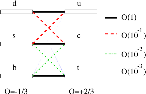
Figure 2.1: Hierarchy of the quark transitions mediated through charged currents.

Wolfenstein Parametrization

In Fig. (2.1), we have illustrated the hierarchy of the strengths of the quark transitions mediated through charged-current interactions: transitions within the same generation are governed by CKM elements of ${\cal O}(1)$, those between the first and the second generation are suppressed by CKM factors of ${\cal O}(10^{-1})$, those between the second and the third generation are suppressed by ${\cal O}(10^{-2})$, and the transitions between the first and the third generation are even suppressed by CKM factors of ${\cal O}(10^{-3})$. In the standard parametrization Eq. (2.37), this hierarchy is reflected by

$$s_{12} = 0.222$$

$$s_{23} = {\cal O}(10^{-2})$$ (2.38)

$$s_{13} = {\cal O}(10^{-3}).$$

If we introduce a set of new parameters $\lambda$, $A$, $\rho$ and $\eta$ by imposing the relations [20, 21]

$$s_{12} \equiv \lambda=0.222,$$

$$s_{23} \equiv A\lambda^{2},$$ (2.39)

$$s_{13}e^{-i\delta_{13}} \equiv A\lambda^{3}(\rho-i\eta),$$

and go back to the standard parametrization Eq. (2.37), we obtain an exact parametrization of the CKM matrix as a function of $\lambda$ (and $A$, $\rho$, $\eta$). Now we can expand straightforwardly each CKM element in the small parameter $\lambda$. Neglecting terms of ${\cal O}(\lambda^{4})$, we arrive at the famous “Wolfenstein parametrization” of the CKM matrix [22]:

$$\hat{V}_{\mbox{{\scriptsize CKM}}}=\left(\begin{array}[]{ccc}1-\frac{1}{2}\lambda^{2}&\lambda&A\lambda^{3}(\rho-i\eta)\\ -\lambda&1-\frac{1}{2}\lambda^{2}&A\lambda^{2}\\ A\lambda^{3}(1-\rho-i\eta)&-A\lambda^{2}&1\end{array}\right)+{\cal O}(\lambda^{4}).$$ (2.40)

Since this parametrization makes the hierarchy of the CKM matrix explicit, it is very useful for phenomenological applications.

2.6.2 Requirements for CP Violation

As we have seen in the previous Section, at least three generations are required to accommodate CP-violation in the Standard Model. However, still more conditions have to be satisfied for observable CP-violating effects. These conditions can be obtained by working in the weak basis and imposing

$$\Phi\equiv\Phi^{\prime}$$

to assure CP invariance in the charged current terms (see Eq. (2.19)). In this case the necessary and sufficient condition for CP invariance is found in Eq. (2.17). Using the matrices

$$H = M\,M^{\dagger}$$

$$H^{\prime} = M^{\prime}\,M^{\prime\dagger}$$

these conditions read

$$\begin{array}[]{rcl}\Phi^{\dagger}H\Phi&=&H^{*}=H^{T}\\ \Phi^{\dagger}H^{\prime}\Phi&=&H^{\prime*}=H^{\prime T}.\end{array}$$ (2.43)

These are necessary and sufficient conditions for CP invariance with any number of generations. In the case of three generations Eq. (2.43) is equivalent to [23]

$$Tr\,[H,H^{\prime}]^{3}=0.$$ (2.44)

To see the physical meaning of this condition we can work in the weak basis where $H$ is diagonal, $H=diag\{m_{u}^{2},m_{c}^{2},m_{t}^{2}\}$, to get

$$(m_{t}^{2}-m_{c}^{2})(m_{c}^{2}-m_{u}^{2})(m_{t}^{2}-m_{u}^{2})\,Im[H^{\prime}_{12}H^{\prime}_{23}H^{\prime}_{31}]=0.$$ (2.45)

It is clear that if we would have chosen to work in the basis where $H^{\prime}$ is diagonal, then we would have obtained a condition analogous to Eq. (2.45) but with the down sector masses and the imaginary part of the $H_{ij}$ elements instead. Therefore we see that a condition for CP invariance is to have no degeneracy in the masses of the up and down sectors. Moreover, it can be seen [24] that Eq. (2.45) contains, beside of the relationship between the masses, the condition of reality of the CKM matrix. Adding up all together we write the necessary and sufficient condition for CP invariance as

$$(m_{t}^{2}-m_{c}^{2})(m_{t}^{2}-m_{u}^{2})(m_{c}^{2}-m_{u}^{2})$$ (2.46)

$$\times(m_{b}^{2}-m_{s}^{2})(m_{b}^{2}-m_{d}^{2})(m_{s}^{2}-m_{d}^{2})\times J_{\rm CP}\,\not=\,0,$$

where

$$J_{\rm CP}=|\mbox{Im}(V_{i\alpha}V_{j\beta}V_{i\beta}^{\ast}V_{j\alpha}^{\ast})|\quad(i\not=j,\,\alpha\not=\beta)\,.$$ (2.47)

The factors in Eq. (2.46) involving the quark masses are related to the fact that the CP-violating phase of the CKM matrix could be eliminated through an appropriate unitary transformation of quark fields if any two quarks with the same charge had the same mass. Consequently, the origin of CP-violation is not only closely related to the number of fermion generations, but also to the hierarchy of quark masses and cannot be understood in a deeper way unless we have insights into these very fundamental issues, usually referred to as the “flavour problem”.

The second ingredient of Eq. (2.46), the “Jarlskog Parameter” $J_{\rm CP}$ [24], is sometimes interpreted as a measure of the strength of CP-violation in the Standard Model. It does not depend on the chosen quark-field parametrization, i.e. is invariant under Eq. (2.28), and the unitarity of the CKM matrix implies that all combinations $|\mbox{Im}(V_{i\alpha}V_{j\beta}V_{i\beta}^{\ast}V_{j\alpha}^{\ast})|$ are equal. Using the Standard and Wolfenstein parameterizations, we obtain

$$J_{\rm CP}=s_{12}s_{13}s_{23}c_{12}c_{23}c_{13}^{2}\sin\delta_{13}=\lambda^{6}A^{2}\eta={\cal O}(10^{-5}),$$ (2.48)

where we have taken into account the present experimental information on the Wolfenstein parameters in the quantitative estimate. Consequently, CP-violation is a small effect in the Standard Model. Typically, new complex couplings are present in scenarios for new physics, yielding additional sources for CP-violation.

2.6.3 The Unitarity Triangles

Concerning tests of the Kobayashi–Maskawa picture of CP-violation, the central targets are the “unitarity triangles” of the CKM matrix. The unitarity of the CKM matrix, which is described by

$$\hat{V}_{\mbox{{\scriptsize CKM}}}^{\,\,\dagger}\cdot\hat{V}_{\mbox{{\scriptsize CKM}}}=\hat{1}=\hat{V}_{\mbox{{\scriptsize CKM}}}\cdot\hat{V}_{\mbox{{\scriptsize CKM}}}^{\,\,\dagger},$$ (2.49)

implies a set of 12 equations, consisting of 6 normalization relations and 6 orthogonality relations. Of particular interest are the 6 orthogonality relations:

$$V_{ud}V_{us}^{\ast}+V_{cd}V_{cs}^{\ast}+V_{td}V_{ts}^{\ast} = 0\quad\mbox{[1st and 2nd column]}$$ (2.50)

$$V_{ud}V_{ub}^{\ast}+V_{cd}V_{cb}^{\ast}+V_{td}V_{tb}^{\ast} = 0\quad\mbox{[1st and 3nd column]}$$ (2.51)

$$V_{us}V_{ub}^{\ast}+V_{cs}V_{cb}^{\ast}+V_{ts}V_{tb}^{\ast} = 0\quad\mbox{[2nd and 3rd column]}$$ (2.52)

$$V_{ud}^{\ast}V_{cd}+V_{us}^{\ast}V_{cs}+V_{ub}^{\ast}V_{cb} = 0\quad\mbox{[1st and 2nd row]}$$ (2.53)

$$V_{ub}^{\ast}V_{tb}+V_{us}^{\ast}V_{ts}+V_{ud}^{\ast}V_{td} = 0\quad\mbox{[1st and 3rd row]}$$ (2.54)

$$V_{cd}^{\ast}V_{td}+V_{cs}^{\ast}V_{ts}+V_{cb}^{\ast}V_{tb} = 0\quad\mbox{[2nd and 3rd row].}$$ (2.55)

These can be represented as six “unitarity triangles” in the complex plane [25] – see Fig. (2.2). It should be noted that the set of Eqs. (2.50)–(2.55) is invariant under the phase transformations specified in Eq. (2.28). If one performs such transformations, the triangles corresponding to Eqs. (2.50)–(2.55) are rotated as a whole in the complex plane. However, the angles and sides of these triangles remain unchanged and are therefore physical observables. It can be shown that all six unitarity triangles have the same area [26], which is given by the Jarlskog parameter as follows:

$$A_{\Delta}=\frac{1}{2}J_{\rm CP}.$$ (2.56)

Figure 2.2: Unitarity triangle for the $bd$ sector where all sides are the same order of magnitude in the Wolfenstein parameter, namely $\lambda^{3}$.

The shape of the unitarity triangles can be analyzed with the help of the Wolfenstein parametrization, implying the following structure for (2.50)–(2.52) and (2.53)–(2.55) respectively:

$${\cal O}(\lambda)+{\cal O}(\lambda)+{\cal O}(\lambda^{5}) = 0\ \ \ [ds-\mbox{triangle}]$$ (2.57)

$${\cal O}(\lambda^{3})+{\cal O}(\lambda^{3})+{\cal O}(\lambda^{3}) = 0\ \ \ [bd-\mbox{triangle}].$$ (2.58)

$${\cal O}(\lambda^{4})+{\cal O}(\lambda^{2})+{\cal O}(\lambda^{2}) = 0\ \ \ [bs-\mbox{triangle}]$$ (2.59)

Where for purposes of this work we have remarked only to which triangle of the down sector corresponds each relationship.

It is clear that the $ds$ and $bs$-triangles are much flatter than the $bd$-triangle, and this will have important consequences. As a matter of fact we will show in Chapter 5 how it is possible to take profit of it working in the Lagrangian only up to a given order in $\lambda$. The rest could be worked out in perturbation theory.

Chapter 3 The neutral meson system

Throughout history the first neutral meson system to be known was the Kaon system, first discovered by Rochester and Butler in 1947 [27]. These particles, the $K^{0}$ and ${\bar{K}}^{0}$, with the respective quark composition $d{\bar{s}}$ and ${\bar{d}}s$, have a very special feature: they are strong interactions eigenstates which decay and may get converted one into the other through weak interactions. The consequences of this feature are rich in the purpose of testing CP-violation in the weak interactions. Since these particles decay through weak interactions they have relatively long lifetimes. And since they can be mixed also through weak interactions, any decay of one of the mesons with time evolution will include the interference diagram of the other one. In this way, if the charged current weak Hamiltonian, responsible of the mixing between $K^{0}$ and $\bar{K}^{0}$, is not invariant under $any$ of the CP operators defined in Eq. (2.34) then CP-violating decays will occur in the $K^{0}-{\bar{K}}^{0}$ system.

With the later discovery of heavier quarks, other similar meson systems were predicted and discovered, the following table summarizes the situation

meson system	particles	quark composition
Kaons	$K^{0},\ {\bar{K}}^{0}$	$d{\bar{s}},\ {\bar{d}}s$
charmed mesons	$D^{0},\ {\bar{D}}^{0}$	$c\bar{u},\ \bar{c}u$
bottom mesons	$B^{0},\ \bar{B^{0}}$	$d\bar{b},\ \bar{d}b$
bottom strange mesons	$B^{0}_{s},\ \bar{B^{0}}_{s}$	$s\bar{b},\ \bar{s}b$
	Table $3.1$

3.1 The formalism for the decays in the neutral meson system

In 1955 Gell-Mann and Pais [28] developed the theory for the neutral Kaon system, which can be adapted for all the neutral meson systems. The Kaon decays should exhibit unusual and peculiar properties arising from the degeneracy of $K^{0}$ and ${\bar{K}}^{0}$. Although $K^{0}$ and ${\bar{K}}^{0}$ are expected to be distinct particles from the point of view of strong interactions, they could transform into each other through the action of weak interactions. Consequently, $K^{0}$ or ${\bar{K}}^{0}$ particles are not expected to decay in the simple exponential manner usually associated with unstable particles, instead they are rather described through the Weisskopf-Wigner [29] formalism. We describe now the results and tools of such a formalism.

For the sake of clarity from now on we will not refer to an specific meson system, but instead we will describe the two particles of any of the meson system of Table $3.1$ as $P^{0}$ and ${\bar{P}}^{0}$.

3.1.1 Time evolution in the Weisskopf-Wigner approximation

The Weisskopf-Wigner approximation is applicable for two particles $P^{0}$ and ${\bar{P}}^{0}$ which are unstable and decay through a different variety of channels. The Weisskopf-Wigner formalism shows that once the decay channels that connect the different particles are integrated out, the picture can be understood with the help of a non-hermitian effective Hamiltonian, $H$, which is responsible of the time evolution and decay of these particles.

The different components of the $H$ $2\times 2$-matrix in the $P^{0},\,{\bar{P}}^{0}$ basis are

$$\begin{array}[]{lc}H_{ij}=\langle P^{0}_{i}|H|P^{0}_{j}\rangle,&P^{0}_{1}=P^{0}\,\ \ P^{0}_{2}={\bar{P}}^{0}\end{array}$$ (3.2)

Notice at this point that there is a non-global phase indeterminacy in the $H_{ij}$ elements. This is due to the fact that the $|{\bar{P}}^{0}\rangle$ state has a free phase which comes from having the CP-operator defined up to the phase matrices $\Theta$ as far as the weak Hamiltonian is not included. In this Chapter this indeterminacy will remain, meanwhile in Chapter 5 we will see how we can get rid of this indeterminacy through a useful choice of the CP operator.

Since $H$ contains as well the evolution as the decay information of the meson system, it must contain an hermitian and anti-hermitian part, $\mbox{\boldmath$H$}=\mbox{\boldmath$M$}-i/2\mbox{\boldmath$\Gamma$}$ where

$$\mbox{\boldmath$M$}=\frac{\mbox{\boldmath$H$}+\mbox{\boldmath$H$}^{\dagger}}{2}\ \ \ \mbox{and}\ \ -i\mbox{\boldmath$\Gamma$}/2=\frac{\mbox{\boldmath$H$}-\mbox{\boldmath$H$}^{\dagger}}{2},$$ (3.3)

both $M$ and $\Gamma$ hermitian matrices.

The time-evolution of any state living in the 2-dimensional vector-space of $P^{0},\,{\bar{P}}^{0}$ will be given through the time-evolving Weisskopf-Wigner eigenstates. Id est, the two eigenvectors of $H$, namely $P^{{}^{(WW)}}_{1}$ and $P^{{}^{(WW)}}_{2}$ with corresponding eigenvalues $\mu_{1}$ and $\mu_{2}$ evolve in time according to the Schrodinger equation

$$H|P^{{}^{(WW)}}_{\alpha}\rangle=\mu_{\alpha}|P^{{}^{(WW)}}_{\alpha}\rangle$$ (3.4)

which implies a time evolution through the non-unitary evolution operator matrix

$$U(t)\,|P^{{}^{(WW)}}_{\alpha}\rangle=e^{-i\mu_{\alpha}t}\,|P^{{}^{(WW)}}_{\alpha}\rangle\ \ \ \ \alpha=1,\,2.$$ (3.5)

(The notation is such that Greek indices indicate a Weisskopf-Wigner eigenstate meanwhile Latin indices indicate a flavour state.) Any given linear combination of them evolves as the same linear combination of the eigenstates evolved. Of course, since the $\mu_{\alpha}\equiv m_{\alpha}-i\,\Gamma_{\alpha}/2$ are complex, this time evolution implies a non-conservation of the probability which is due to the fact that the states living in this vector-space are unstable.

In this way all the time evolution of the system is reduced to find $H$’s eigenvectors and write the state function, $|\psi\rangle$, as a linear combination of them. Any confusion that might arise from the fact of having non-orthonormal eigenvectors will be clarified in the next paragraphs.

Generally speaking, when working with a non-orthonormal basis it is necessary to differentiate between $coordinate$ and $component$ of a vector in a given basis. Id est, given a state function that may be written as

$$|\psi\rangle=\lambda_{1}|P^{{}^{(WW)}}_{1}\rangle+\lambda_{2}|P^{{}^{(WW)}}_{2}\rangle,$$ (3.6)

we say that $\lambda_{1}$ and $\lambda_{2}$ are the $coordinates$ of $|\psi\rangle$ on the vector basis. Meanwhile, the $components$ of the vector on such a basis are $\eta_{1}=\langle P^{{}^{(WW)}}_{1}|\psi\rangle$ and $\eta_{2}=\langle P^{{}^{(WW)}}_{2}|\psi\rangle$. If the basis $\{P^{{}^{(WW)}}_{\alpha}\}$ is non-orthonormal then $\lambda_{\alpha}\neq\eta_{\alpha}$.

Once this is clear we realize that for the time evolution of any given state-function it is necessary to extract the $coordinates$ of it. For the sake of concreteness in the following we write the eigenvectors of $H$ as

$$\left(\begin{array}[]{c}|P^{{}^{(WW)}}_{1}\rangle\\ |P^{{}^{(WW)}}_{2}\rangle\end{array}\right)=\left(\begin{array}[]{cc}p_{1}&q_{1}\\ p_{2}&-q_{2}\end{array}\right)\ \left(\begin{array}[]{c}|P^{0}\rangle\\ |{\bar{P}}^{0}\rangle\end{array}\right)\equiv\mbox{\boldmath$X$}^{T}\ \left(\begin{array}[]{c}|P^{0}\rangle\\ |{\bar{P}}^{0}\rangle\end{array}\right).$$ (3.15)

As a result, the coordinates of any vector $|\psi\rangle$ in the Weisskopf-Wigner basis are

$$\lambda_{\alpha}=\left(\mbox{\boldmath$X$}^{\dagger}\mbox{\boldmath$X$}\right)^{-1}_{\alpha\beta}\langle P^{{}^{(WW)}}_{\beta}|\psi\rangle.$$ (3.16)

The state into which $|\psi\rangle$ is being projected in Eq. (3.16),

$$|\tilde{P}^{{}^{(WW)}}_{\alpha}\rangle=\left(\mbox{\boldmath$X$}^{T}\mbox{\boldmath$X$}^{*}\right)^{-1}_{\alpha\beta}|P^{{}^{(WW)}}_{\beta}\rangle=X^{*-1}_{\alpha i}|P^{0}_{i}\rangle,$$ (3.17)

may be found in the literature under the name of reciprocal basis [30] or out-state [31]. We recall that in terms of $P^{0}$ and ${\bar{P}}^{0}$ the particle composition of $\tilde{P}^{{}^{(WW)}}_{\alpha}$ differs from that of $P^{{}^{(WW)}}_{\alpha}$. In fact, the reciprocal basis, or out-state basis $\{\tilde{P}^{{}^{(WW)}}_{\alpha}\}$, has no physical meaning, it is only a tool to extract the coordinates of any given vector and that is the only use that shall be given to it.

As it can be easily seen from Eq. (3.17) the reciprocal basis will differ from the regular basis only in the case that the set of eigenvectors of the Hamiltonian is not orthogonal. Notice that the non-orthogonality of $H$’s eigenvectors is not necessarily a consequence of non-hermiticity; the causes are analyzed in the following paragraphes.

The operator for the effective Hamiltonian is written as

$$H = |P^{{}^{(WW)}}_{1}\rangle\mu_{1}\langle\tilde{P}^{{}^{(WW)}}_{1}|+|P^{{}^{(WW)}}_{2}\rangle\mu_{2}\langle\tilde{P}^{{}^{(WW)}}_{2}|$$ (3.22)

$$= \left(|P^{{}^{(WW)}}_{1}\rangle,\,|P^{{}^{(WW)}}_{2}\rangle\right)\left(\begin{array}[]{cc}\mu_{1}&0\\ 0&\mu_{2}\end{array}\right)\left(\begin{array}[]{c}\langle\tilde{P}^{{}^{(WW)}}_{1}|\\ \langle\tilde{P}^{{}^{(WW)}}_{2}|\end{array}\right).$$

Id est, the Hamiltonian is being diagonalized through the eigenvectors’ matrix as

$$\mbox{\boldmath$X$}^{-1}\mbox{\boldmath$H$}\mbox{\boldmath$X$}=\left(\begin{array}[]{cc}\mu_{1}&0\\ 0&\mu_{2}\end{array}\right)$$ (3.25)

Using the reciprocal basis Eq. (3.17) to extract the coordinates of the state-function, it is easy now to get the time evolution due to the Schrodinger Equation (Eq. (3.4)):

$$|\psi(t)\rangle=\left[e^{-i\mu_{1}t}\langle\tilde{P}^{{}^{(WW)}}_{1}|\psi(0)\rangle\right]|P^{{}^{(WW)}}_{1}\rangle+\left[e^{-i\mu_{2}t}\langle\tilde{P}^{{}^{(WW)}}_{2}|\psi(0)\rangle\right]|P^{{}^{(WW)}}_{2}\rangle.$$ (3.26)

3.1.2 T, CP and CPT analysis in the time evolution (mixing)

In the previous section the time evolution of the neutral meson states has been obtained within the Weisskopf-Wigner approximation. All the information for such evolution is contained in the effective Hamiltonian $H$ matrix or, alternatively, in the eigenvectors matrix $X$. In this section we study the different properties of these two matrices and their relationship to the discrete symmetries in the time evolution, which will prove to be useful for a better understanding of the system.

To begin the analysis, we first show how the symmetry-operations C, P, and T on $H$ have immediate consequences on the matrix $H$ written in the flavour basis. Acting on each matrix element we find,

$$\mbox{CPT}^{\sqrt{}}\ \Longrightarrow \mbox{\boldmath$H$}_{11}=\mbox{\boldmath$H$}_{22}$$ (3.27)

$$\mbox{CP}^{\sqrt{}}\ \Longrightarrow \mbox{\boldmath$H$}_{11}=\mbox{\boldmath$H$}_{22}\mbox{ and }|\mbox{\boldmath$H$}_{12}|=|\mbox{\boldmath$H$}_{21}|$$ (3.28)

$$\mbox{T}^{\sqrt{}} \Longrightarrow |\mbox{\boldmath$H$}_{12}|=|\mbox{\boldmath$H$}_{21}|$$ (3.29)

where the moduli are due to the relative phase indeterminacy between the $|P^{0}\rangle$ and $|{\bar{P}}^{0}\rangle$ states.

The eigenvectors of $H$ should be simultaneously eigenstates of CP if this were a good symmetry. Instead, under CP, T and CPT violation, the matrix $\mbox{\boldmath$X$}^{T}$ in Eq. (3.15) can be parameterized as

$$\mbox{\boldmath$X$}^{T}=\left(\begin{array}[]{cc}p_{1}&q_{1}\\ p_{2}&-q_{2}\end{array}\right)=\left(\begin{array}[]{cc}1+\epsilon_{1}&1-\epsilon_{1}\\ 1+\epsilon_{2}&-(1-\epsilon_{2})\end{array}\right),$$ (3.34)

where the obvious normalization constants in each row are not put in order to avoid visual saturation. It should be clear that these parameters are rephasing-variant, id est changes in the relative phases of the states are reflected in a change in the epsilons. This indeterminacy will be removed in Chapter 5 when the ${\bar{P}}^{0}(=\bar{B}^{0})$ state is defined through a given $CP$-operator.

The physical meaning of the parametrization in Eq. (3.34) is clear, assuming $|{\bar{P}}^{0}\rangle=\mbox{CP}\,|P^{0}\rangle$, $H$’s eigenvectors are parameterized as almost $CP$ eigenvectors as far as $\epsilon_{1,2}$ are small, id est

$$|P^{{}^{(WW)}}_{1}\rangle = |P^{0}_{+}\rangle+\epsilon_{1}P^{0}_{-}\rangle$$ (3.35)

$$|P^{{}^{(WW)}}_{2}\rangle = |P^{0}_{-}\rangle+\epsilon_{2}P^{0}_{+}\rangle$$ (3.36)

where

$$|P^{0}_{{}^{+}_{-}}\rangle=\frac{1}{\sqrt{2}}\left(P^{0}\pm{\bar{P}}^{0})\right)$$ (3.37)

(It is clear that if $\epsilon_{1,2}$ are not small, the parametrization is still valid and general.)

In order to have a more direct connection between the discrete symmetries and the parameters, it is convenient to define

$$\epsilon=\frac{\epsilon_{1}+\epsilon_{2}}{2}\ \ \ \ \ \ \ \ \ \ \delta=\frac{\epsilon_{1}-\epsilon_{2}}{2}.$$ (3.38)

In this way the T, CP and CPT symmetries or violations can be easily parameterized. It is convenient to note at this point that if, as supported by experiments [32], $\delta$ is very small compared to $\epsilon$, then $Re(\epsilon)\neq 0$ is needed to guarantee that $\epsilon$ cannot be rephased to zero. In fact, it is easy to see that if we have $\epsilon=i\,x$ then the rephase

$$\begin{array}[]{c}P^{0}\to P^{0}e^{-i\arctan(x)}\\ {\bar{P}}^{0}\to{\bar{P}}^{0}e^{i\arctan(x)}\end{array}$$ (3.41)

makes $\epsilon=0$ in Eqs. (3.35-3.36).

To analyze the relationship between the parameters ($\epsilon,\delta$) and the discrete symmetries it is instructive to compute the evolution operator matrix in the flavour basis $\left\{P^{0},{\bar{P}}^{0}\right\}$, which reads

$$U(t) = X\left(\begin{array}[]{cc}e^{-i\mu_{1}t}&0\\ 0&e^{-i\mu_{2}t}\end{array}\right)X^{-1}$$ (3.44)

$$= e^{-(i\bar{m}+\frac{\Gamma}{2})t}\left(\begin{array}[]{ll}\cosh(\alpha t)-K_{\delta}\sinh(\alpha t)&-K_{+}\sinh(\alpha t)\\ -K_{-}\sinh(\alpha t)&\cosh(\alpha t)+K_{\delta}\sinh(\alpha t)\\ \end{array}\right)$$ (3.47)

where

$$\alpha = i\frac{\Delta m}{2}+\frac{\Delta\Gamma}{4},$$

$$K_{\pm} = \frac{(1\pm\epsilon)^{2}-\delta^{2}}{1-\epsilon^{2}+\delta^{2}}$$ (3.48)

$$K_{\delta} = \frac{2\delta}{1-\epsilon^{2}+\delta^{2}},$$ (3.49)

$\Delta\Gamma=\Gamma_{1}-\Gamma_{2},\ \Delta m=m_{1}-m_{2},\ \Gamma=(\Gamma_{1}+\Gamma_{2})/2$ and $\bar{m}=(m_{1}+m_{2})/2$.

Under a rephasing of the states $B^{0}\mapsto e^{i\gamma},\ \bar{B^{0}}\mapsto e^{-i\bar{\gamma}}$ the parameters rephase as

$$K_{\pm} \mapsto K_{\pm}e^{\pm i(\gamma-\bar{\gamma})}$$ (3.50)

$$K_{\delta} \mapsto K_{\delta}.$$ (3.51)

Hence, there are five rephasing invariant parameters ($|K_{+}|,\ |K_{-}|$, $Re(K_{\delta})$, $Im(K_{\delta})$ and the phase of $K_{+}K_{-}$) which, due to the two real relationships contained in

$$K_{+}\,K_{-}=1-K_{\delta}^{2},$$ (3.52)

get reduced to three physical parameters.

In terms of $\epsilon$ and $\delta$ the number of parameters must be the same. In particular this is easily seen for the case of $B_{d}$ mesons where a small $\Delta\Gamma$ implies a small $Re(\epsilon)$ (see the demonstration below). In this case, we have that to first order in $Re(\epsilon)$ and $\delta$, Eqs. (3.48) and (3.49) say

$$|K_{\pm}|^{2} = 1\pm\frac{4Re(\epsilon)}{1+|\epsilon|^{2}},$$

$$K_{\delta} = \frac{2\delta}{1+|\epsilon|^{2}},$$

and hence the three physical parameters which are rephasing invariant in this approximation (valid for the $B_{d}$-system) are

$$\left\{\frac{Re(\epsilon)}{1+|\epsilon|^{2}},\,\frac{Re(\delta)}{1+|\epsilon|^{2}},\,\frac{Im(\delta)}{1+|\epsilon|^{2}}\right\}\longrightarrow\mbox{rephasing invariants}$$ (3.53)

It is worth to note at this point that if, as in Chapter 5, the relative phase of the states is defined by a CP-conserving direction then the four parameters included in $\epsilon$ and $\delta$ would have physical meaning; id est, $Im(\epsilon)/1+|\epsilon|^{2}$ should be added in Eq. (3.53).

With the evolution operator written explicitly in the flavour basis (see Eq. (3.44)), the T, CP and CPT transformed expressions of $U(t)$ are obtained straightforward. In fact, the T operation transposes the $U(t)$ matrix; the CP operation transposes it and exchanges $U_{11}\leftrightarrow U_{22}$; and the CPT operation exchanges $U_{11}\leftrightarrow U_{22}$. Therefore, from the matrix expression of the $U$-operator we obtain the behaviour of the T, CP and CPT transformed operator as a function of $\epsilon$ and $\delta$:

$$\mbox{T}\,U(\epsilon,\delta)\,\mbox{T}^{\dagger} = U(-\epsilon,\delta)$$ (3.54)

$$\mbox{CP}\,U(\epsilon,\delta)\,\mbox{CP}^{\dagger} = U(-\epsilon,-\delta)$$ (3.55)

$$\mbox{CPT}\,U(\epsilon,\delta)\,\mbox{CPT}^{\dagger} = U(\epsilon,-\delta)$$ (3.56)

From here, having into account that $Re(\epsilon)\neq 0$ is the requirement to guarantee that $\epsilon$ cannot be rephased to zero (see Eq. (3.41)), the relationship between the parameters and the discrete symmetries in the time evolution (mixing) follows

$$\mbox{T}^{\sqrt{}} \iff Re(\epsilon)=0,$$ (3.57)

$$\mbox{CP}^{\sqrt{}} \iff Re(\epsilon)=0\mbox{ and }\delta=0,$$ (3.58)

$$\mbox{CPT}^{\sqrt{}} \iff \delta=0.$$ (3.59)

It is also useful to see the implications of measuring a non-zero value for one of the parameters,

$$Re(\epsilon)\neq 0 \Longrightarrow$$ and (3.60)

$$\delta\neq 0 \Longrightarrow \begin{picture}(2.0,1.0)\mbox{\scriptsize CP}\put(-1.6,-0.1){\line(2,1){1.7}}\end{picture}\mbox{ and }\begin{picture}(2.0,1.0)\mbox{\scriptsize CPT}\put(-2.4,-0.1){\line(3,1){2.5}}\end{picture}.$$ (3.61)

Conclusions in Eqs. (3.57-3.61) are general and their understanding implies a good insight into the formalism of the neutral meson system.

It is also interesting to obtain the Hamiltonian operator parameterized in the flavour basis. This is easily done using the expression for the evolution operator in Eq. (3.44) and the expansion for small $t$

$$U(t)\approx 1-iHt;$$ (3.62)

we obtain

$$H=\left(\begin{array}[]{cc}\bar{m}-i\frac{\Gamma}{2}-iK_{\delta}\,\alpha&-iK_{+}\,\alpha\\ -iK_{-}\,\alpha&\bar{m}-i\frac{\Gamma}{2}+iK_{\delta}\,\alpha\end{array}\right).$$ (3.65)

Up to here we have worked with $\epsilon$ and $\delta$ at the same level. In nature, though, CP and T violations are much greater than CPT violation (if any). Hence, in virtue of Eqs. (3.57-3.59) we can work out interesting conclusions approximating $\delta\approx 0$. In fact, when studying T and CP violation this is an excellent approximation. In the remaining of this Section we assume CPT invariance, and thus $\epsilon=\epsilon_{1}=\epsilon_{2}$.

Notice, in Eq. (3.34), that if CPT is assumed then $p_{1}=p_{2}\equiv p$ and $q_{1}=q_{2}\equiv q$ and $\mbox{\boldmath$X$}^{T}$ is simply

$$\mbox{\boldmath$X$}^{T}=\left(\begin{array}[]{cc}p&q\\ p&-q\end{array}\right).$$ (3.66)

Moreover $p$ and $q$ values in term of $H$’s elements are trivial,

$$\frac{q}{p}=\pm\sqrt{\frac{H_{21}}{H_{12}}},$$ (3.67)

where the $\pm$ sign comes from the two different eigenvectors. A later assignment – through the eigenvalues – of the eigenvectors to each column of $X$ will eliminate this indeterminacy.

Taking the positive sign in Eq. (3.67) and using Eq. (3.34) yields

$$\epsilon=\frac{\sqrt{H_{12}}-\sqrt{H_{21}}}{\sqrt{H_{12}}+\sqrt{H_{21}}}.$$ (3.68)

It is interesting to notice that for the case of the neutral mesons having similar mean-lives – as with the $B_{d}$ – the expression in Eq. (3.68) can be expanded in terms of the small rephasing-invariant parameter $\frac{\Gamma_{21}}{2M_{21}}$. The result, renormalized to $1+|\epsilon|^{2}$, is

$$\frac{Re\,\epsilon}{1+|\epsilon|^{2}} = \frac{1}{2}Im\left(\frac{\Gamma_{21}}{2M_{21}}\right)+O\left(\left[\frac{\Gamma_{21}}{2M_{21}}\right]^{2}\right)$$ (3.69)

$$\frac{Im\,\epsilon}{1+|\epsilon|^{2}} = -\frac{1}{2}\sin\phi+O\left(\frac{\Gamma_{21}}{2M_{21}}\right)$$ (3.70)

where $M_{21}=|M_{21}|e^{i\phi}$. As we see, we retrieve again that while Eq. (3.70) is phase dependent, Eq. (3.69) is rephasing-invariant. Also notice that in Eq. (3.69) we have the proof that for small $\Delta\Gamma$, $Re(\epsilon)$ is also small and proportional to it.

Also a different expression for $\epsilon$ may be obtained through the elements of $\Gamma$ and $M$. Using that the eigenvalues of $H$ accomplish

$$2\sqrt{H_{12}H_{21}}=\mu_{1}-\mu_{2}=\Delta m-\frac{i}{2}\Delta\Gamma$$ (3.71)

in Eq. (3.68) it is straightforward to get

$$\epsilon=\frac{Im(\Gamma_{12})+2iIm(M_{12})}{2Re(M_{12})-iRe(\Gamma_{12})+\Delta m-\frac{i}{2}\Delta\Gamma}.$$ (3.72)

Also, from the real and imaginary part of the square of Eq. (3.71) other two practical relations may be obtained, namely

$$|M_{12}|^{2}-\frac{1}{4}|\Gamma_{12}|^{2} = \Delta m\,^{2}-\frac{1}{4}\Delta\Gamma\,^{2}$$ (3.73)

$$Re\left(\Gamma_{12}M_{12}^{*}\right) = \Delta m\,\Delta\Gamma.$$ (3.74)

At last, in order to recompile the relationship between all the variables and parameters in game, we analyze the non-orthogonality of the Weisskopf-Wigner eigenstates . Assuming CPT invariance, the internal product of the two Weisskopf-Wigner eigenstates is directly proportional to

$$\langle P^{{}^{(WW)}}_{1}|P^{{}^{(WW)}}_{2}\rangle\propto 1-\left|\frac{H_{12}}{H_{21}}\right|\propto 4Re\,\epsilon.$$ (3.75)

Hence the real part of $\epsilon$ is also directly related to the non-orthogonality of the eigenvectors. Besides this, another relationships can be found by studying the causes for $|H_{12}|\neq|H_{21}|$ or $|H_{12}|=|H_{21}|$ with the matrices $M$ and $\Gamma$. It is easy to see that

$$|H_{12}|=|H_{21}|\ \iff\ Im(M_{12}\Gamma_{12}^{*})=0.$$ (3.76)

Moreover, for CPT${}^{\sqrt{}}$ it is valid that

$$Im(M_{12}\Gamma_{12}^{*})=0\iff[M,\Gamma]=0.$$ (3.77)

On the other hand, for the mass and life-time difference the implication is only one way,

$$M_{12}\ (or\ \Gamma_{12})=0\Longrightarrow\left\{\begin{array}[]{l}Im(M_{12}\Gamma_{12}^{*})=0\\ \Delta m\ (or\ \Delta\Gamma)=0.\end{array}\right.$$ (3.78)

We can summarize all the information by writing

$$\left.\begin{array}[]{l}\begin{picture}(2.0,1.0)\mbox{\scriptsize CP}\put(-1.6,-0.1){\line(2,1){1.7}}\end{picture}\mbox{ in the mixing}\\ \begin{picture}(1.0,1.0)\mbox{\scriptsize T}\put(-1.0,-0.08){\line(2,1){1.3}}\end{picture}\mbox{ in the mixing}\\ Re(\epsilon)\neq 0\\ \frac{|H_{12}|}{|H_{21}|}\neq 1\\ \langle P^{{}^{(WW)}}_{1}|P^{{}^{(WW)}}_{2}\rangle\neq 0\\ ~{}[M,\Gamma]\neq 0\\ Im(M_{12}\Gamma_{12}^{*})\neq 0\end{array}\right\}\mbox{ ~{} ~{} are equivalent (if CPT ${}^{\sqrt{}}$),}$$ (3.86)

If, on the contrary, CPT would be violated then the analysis should be redone on the same steps (easy, but carefully): for instance, we might have but $Re(\epsilon)=0$, since it might be T${}^{\sqrt{}}$.

3.2 The correlated neutral meson system

As a last section in the study of the meson system, we describe and analyze the so called correlated neutral meson system. This is a very important topic, since a great part of the Kaon and $B$-meson experiments are performed nowadays in a correlated preparation at the Phi and B factories, respectively.

These factories began operating around 1999, and since then the B factories (PEP-II and KEK-B) have exceeded their design peak luminosity and greatly exceeded the expected integrated luminosity, whereas the DAFNE Phi factory is still about a factor 5 below the design peak and total integrated luminosity [33]. We study here how the B factories produce correlated pairs of $B$-mesons, the $B^{0}\bar{B^{0}}$ initial state and the notion of tagging; the working of the Phi factories is analogous but, instead, produces pairs of correlated Kaons.

The essence of a B factory is to create in an asymmetric electron-positron collider the upsilon $(4S)$ meson,

$$e\,+\,\bar{e}\to\Upsilon(4S).$$

This is achieved by running the facility at an energy in the center of mass system equal to the mass of the $\Upsilon(4S)$. Once the $\Upsilon(4S)$ has been created, its decay is more than 96% of the times, through the Strong Interactions, to a $B\bar{B}$ pair, and from it half of the times corresponds to a correlated neutral $B^{0}\bar{B^{0}}$ pair [32].

The interesting physics for the purposes of this work comes out when the B mesons are neutral. In this case they mix each other and are indistinguishable in their weak decays, since there is no superselection rule to distinguish them, and therefore they must obey Bose statistics. The indistinguishability implies that the physical neutral meson-antimeson state must be $symmetric$ under the combined operation $C{\cal P}$, with $C$ the charge conjugation and ${\cal P}$ the operator that permutes the spatial coordinates. Specifically, assuming conservation of angular momentum, and a proper existence of the $antiparticle$ $state$, one observes that for $B^{0}\bar{B^{0}}$ states which are $C$ conjugates with $C=(-1)^{\ell}$ (with $\ell$ the angular momentum quantum number), the system has to be an eigenstate of ${\cal P}$ with eigenvalue $(-1)^{\ell}$. Hence, for $\ell=1$ (from the spin of the $\Upsilon$), we have that $C=-$, implying ${\cal P}=-$. As a result the initial correlated state $B^{0}\bar{B^{0}}$ produced in a B factory can be written as

$$|i\rangle=\frac{1}{\sqrt{2}}\left(|B^{0}(-\vec{k}),\bar{B}^{0}(\vec{k})\rangle-|\bar{B}^{0}(-\vec{k}),B^{0}(\vec{k})\rangle\right),$$ (3.87)

where $\vec{k}$ is along the direction of the momenta of the mesons in the center of mass system. A system in a state as Eq. (3.87) is called a correlated neutral $B$-meson system.

To summarize and for future purposes, we remark that Eq. (3.87) was obtained using:

1. conservation of angular momentum in the $\Upsilon(4S)\to B^{0}\,\bar{B^{0}}$ decay,

2. indistinguishability of $B^{0}$ and $\bar{B^{0}}$ in their weak decays, and hence the Bose statistics requirement $C{\cal P}=+$.

The correlation in Eq. (3.87) makes very rich the experimental and theoretical research since a first decay acts as a filter in a quantum mechanical sense and gives a precise preparation for analyzing the second meson still flying. In fact, due to the definite anti-symmetry in Eq. (3.87) the time evolution of the initial state leaves it, up to a global phase which we omit, with its original structure but attenuated by an exponential factor,

$$U(t_{1})\otimes U(t_{1})|i\rangle = e^{-\Gamma t_{1}}|i\rangle$$

$$= e^{-\Gamma t_{1}}\left(\frac{1}{\sqrt{2}}|B^{0}(-\vec{k}),\bar{B}^{0}(\vec{k})\rangle-|\bar{B}^{0}(-\vec{k}),B^{0}(\vec{k})\rangle.\right)$$

Now suppose, for instance, a first decay $B\to X$ at time $t_{1}$, then the state function of the second B meson at that time is projected to

$$e^{-\Gamma t_{1}}\,|B_{\bar{X}}\rangle=\frac{e^{-\Gamma t_{1}}}{\sqrt{2}}\left[\langle X|B^{0}\rangle\,|\bar{B}^{0}\rangle-\langle X|\bar{B}^{0}\rangle\,|B^{0}\rangle\right]$$ (3.89)

which satisfies $\langle X|B_{\bar{X}}\rangle=0$. (As required by Bose statistics, the same decay simultaneously at both sides is not allowed at any time after the creation of the initial state [53].) If the decay product $X$ is flavour specific, we have a flavour tag and we can establish by the conservation law which was the complementary first state $|B_{X}\rangle$ decaying to $X$. The goal in Chapter 5 is to define an analogous tag, but for some CP-eigenstate decays. Id est, a CP-tag.

3.3 Appendix:
On the definition of probability using non-orthogonal basis

As it was studied in Section 3.1, several experimental facts in the neutral meson system may allow to have non-orthogonality in the Weisskopf-Wigner eigenstates, $\langle P^{{}^{(WW)}}_{1}|P^{{}^{(WW)}}_{2}\rangle\neq 0$.

This feature needs a deeper discussion, since it means that when the state is in one of the Weisskopf-Wigner eigenstates, then it has some projection on the other such eigenstate. And thus at first sight, thinking with the usual Quantum Mechanics laws, there could be a transition. In this Section we will try to clarify this issue: we show that if the Weisskopf-Wigner states are assumed to be asymptotic states, then the usual Dirac definition of probability is inconsistent to a gedanken-experiment we propose. In addition, we also show that some other possible generalizations of the definition of probability are also inconsistent, we finally conclude that the Weisskopf-Wigner eigenstates should be taken as intermediate states and not as asymptotic observable states.

3.3.1 The Dirac definition, possible generalizations,
and their problems

Generally speaking, the $\{P^{0},\,{\bar{P}}^{0}\}$ space may be thought as an $n$-dimensional Hilbert space ${\cal H}$, and the state function being $u\rangle\in{\cal H}$. Using the Quantum Mechanic postulates in a gedanken-experiment, we will suppose that if a measure is taken through the Strong Interactions Hamiltonian then the result of measuring an observable distinguishable property of the particle when the state-function is $u\rangle$ must yield that the particle is either $P^{0}$ $or$ ${\bar{P}}^{0}$. Analogously, if in a gedanken-experiment we measure a distinguishable property of the particle then the result must be either $P^{{}^{(WW)}}_{1}$ $or$ $P^{{}^{(WW)}}_{2}$. This gedanken-experiment is the basis of this Appendix.

We will call $\{v_{i}\rangle\}$ the orthogonal basis which describes the $\{P^{0},\ {\bar{P}}^{0}\}$ basis. And we will call $\{v^{\prime}_{i}\rangle\}$ the basis which corresponds to the Weisskopf-Wigner eigenstate basis $\{P^{{}^{(WW)}}_{1},\,P^{{}^{(WW)}}_{2}\}$, which we will assume non-orthogonal. As it can be seen, in order to use a more abstract notation, in this Section we adopt Latin indices for the flavour as well as for the Weisskopf-Wigner basis; the difference between them comes then solely from the not primed and primed vectors, respectively.

In usual Quantum Mechanics, if the system is in the state $u\rangle$ and $v_{i}\rangle$ corresponds to an observable, then the probability of measuring $v_{i}$ is

$$P(v_{i}|u)=|\langle v_{i}|u\rangle|^{2}=\langle u|v_{i}\rangle\langle v_{i}|u\rangle.$$ (3.90)

That is the component of $u\rangle$ on $v_{i}\rangle$, moduli square. This is the case for $\{v_{i}\rangle\}$ orthogonal basis. In this case, the probability amplitude is given by the coordinate, equal to the component, along $v_{i}\rangle$ of the state $u\rangle$.

If, instead, we are dealing with a non orthogonal basis, as $\{v^{\prime}_{i}\rangle\}$ then there are problems of conservation of probability. Let $X$ be the change of basis matrix,

$$v^{\prime}_{j}\rangle=X_{ij}\,v_{i}\rangle.$$ (3.91)

The reciprocal basis, introduced in Eq. (3.17), is then

$$\tilde{v}^{\prime}_{j}=X^{*\,-1}_{ji}\,v_{i}\rangle,$$ (3.92)

and furnishes

$$\langle\tilde{v}^{\prime}_{i},v^{\prime}_{j}\rangle=\delta_{ij}.$$ (3.93)

Once introduced the notation, we propose the following two gedanken-experiments:

$a)$ The state of the system is $u\rangle=v^{\prime}_{j}\rangle$ and we want to have that if we measure one of the $\{v_{i}\rangle\}$ observables with the basis of the Strong Hamiltonian, then we will have either $v_{1}\rangle$ or$\ v_{2}\rangle$ or $\ldots$ or $v_{n}\rangle$. Therefore if all the probabilities are to sum one,

$$\sum_{i}|\langle v_{i}|v^{\prime}_{j}\rangle|^{2}\equiv 1\Longrightarrow\sum_{i}|X_{ij}|^{2}=1\ \ \forall j$$ (3.94)

$b)$ The other way around, $u\rangle=v_{j}\rangle$ and we want to have that if we measure observables that correspond to the basis of the Weisskopf-Wigner effective Hamiltonian, then we will have either $v^{\prime}_{1}\rangle$ or$\ v^{\prime}_{2}\rangle$ or $\ldots$ or $v^{\prime}_{n}\rangle$. Therefore

$$\sum_{i}|\langle v^{\prime}_{i}|v_{j}\rangle|^{2}\equiv 1\Longrightarrow\sum_{i}|X_{ji}|^{2}=1\ \ \forall j.$$ (3.95)

If $X$ is unitary then satisfies Eq. (3.94) and Eq. (3.95), but if $\{v^{\prime}_{i}\rangle\}$ is non-orthogonal then $X$ is non-unitary and –for the case of the neutral mesons– it does not satisfy such conditions. To see this we prove the anti-reciprocal:

Proposition 3.1

If Eq. (3.94) and Eq. (3.95) are accomplished with the $2\times 2$ neutral mesons $X$, Eq. (3.66), then $Re\{\epsilon\}=0$ and thus $X$ is unitary

Dem: quite simple, Eq. (3.94) imposes the known condition for normalization of the eigenstates which, assuming CPT invariance, read

$$|p|^{2}+|q|^{2}=1\Longrightarrow p,q=\frac{1\pm\epsilon}{\sqrt{2(1+|\epsilon|^{2})}}.$$ (3.96)

Meanwhile Eq. (3.95) imposes $2|p|^{2}=2|q|^{2}=1$ therefore $Re\{\epsilon\}=0$ as it was to prove. (q.e.d.)

Notice that this proposition is not true for any non-unitary $X$, there exist even $2\times 2$ non-unitary matrices which accomplish Eqs$.\,$(3.94,3.95).

Therefore we see that, for the neutral meson system, the usual Dirac definition of probability Eq. (3.90) does not conserve the probability in the gedanken-experiment proposed. The sum of the probabilities is not unity.

In order to generalize the definition of probability to non-orthogonal basis the following four reasonable conditions shall be required:

1. let this definition be reduced to the usual Quantum Mechanics’ Dirac probability when the basis happens to be orthogonal;

2. let the probability of any measurement be real;

3. let the probability of any measurement be non-negative;

4. let the experiments $a)$ and $b)$ behave well in the sense that the sum of the probabilities is one.

Since it has been shown that Dirac’s probability does not work for non-orthogonal basis, a second choice is to replace Eq. (3.90) and define the probability as the moduli square of the $coordinates$ as in [30],

P $$= coordinate\cdot coordinate^{*}$$

$$P(v^{\prime}_{i}|u) \equiv |\langle\tilde{v}^{\prime}_{i}|u\rangle|^{2}$$ (3.97)

In this case Eq. (3.94), concerning experiment $a)$, remains the same, but experiment $b)$ instead now implies

$$\sum_{i}|\langle\tilde{v}^{\prime}_{i}|v_{j}\rangle|^{2}=1\rightarrow\sum_{i}|X^{-1}_{ij}|^{2}=1.$$ (3.98)

But if this is true, the following proposition shows that $X$ must be unitary, therefore by reduction ad absurd is proved that this second choice for the definition of probability Eq. (3.97) does not conserve probability for non-unitary $X$.

Proposition 3.2

If $\sum_{i}|X_{ij}|^{2}=\sum_{i}|X^{-1}_{ij}|^{2}=1$ for all $j$, then $X$ is unitary.

Dem: first note that

$$\left.\begin{array}[]{rcl}(v,v)&=&1\\ (v,w)&=&1\\ v&\neq&w\end{array}\right\}\Longrightarrow\ (w,w)>1.$$

In fact, since $w\neq v$ is valid the strict inequality $|w|^{2}+|v|^{2}>2Re\{(w,v)\}$. Therefore using the other two hypothesis we get $|w|^{2}=(w,w)>1$, as it was to show in Eq. (3.3.1).

In order to prove the proposition it is enough to prove the following:

$$\left.\begin{array}[]{l}i)\mbox{\boldmath$X$}\mbox{ is not unitary}\\ ii)\sum_{i}|X_{ij}|^{2}=1\ \forall j\end{array}\right\}\Longrightarrow\exists j/\sum_{i}|X^{-1}_{ij}|\neq 1.$$

Using $i)$ we know that exist $i_{0}$ and $j_{0}$ such that

$$X^{-1}_{i_{0}j_{0}}\neq X^{*}_{j_{0}i_{0}}.$$ (3.99)

Therefore if $v_{j}=X^{*}_{ji_{0}}$ and $w_{j}=X^{-1}_{i_{0}j}$ then $ii)$ implies $(v,v)=1$, and $X^{-1}\cdot X=1$ implies $(v,w)=1$. Since $v\neq w$ because of Eq. (3.99), using Eq. (3.3.1) we get that $(w,w)>1$, that is

$$\sum_{j}|X^{-1}_{i_{0}j}|^{2}>1.$$ (3.100)

If instead is $i^{\prime}_{0}$ such that $X^{-1}_{i^{\prime}_{0}j}=X^{*}_{ji^{\prime}_{0}}\ (j=1\ldots n)$ then

$$\sum_{j}|X^{-1}_{i^{\prime}_{0}j}|^{2}=1.$$ (3.101)

Summing over all the cases of Eq. (3.100) and Eq. (3.101) we get

$$\sum_{i,j}|X^{-1}_{ij}|^{2}>n.$$ (3.102)

Therefore exists at least one $j$ such that

$$\sum_{i}|X^{-1}_{ij}|^{2}\neq 1.$$ (3.103)

And this proves the proposition (q.e.d.).

Motivated by this failure, we attempt a third try to define the probability in such a way that condition $iv)$ is furnished. The next possibility which, in a symmetrical way automatically furnishes condition $ii)$, is

P $$= \frac{1}{2}(coordinate\cdot component^{*}+coordinate^{*}\cdot component)$$

$$P(v_{i}|u) \equiv {1\over 2}\left(\langle u|v_{i}\rangle\langle\tilde{v}^{\prime}_{i}|u\rangle+\langle u|\tilde{v}^{\prime}_{i}\rangle\langle v_{i}|u\rangle\right).$$ (3.104)

With this definition we see that experiment $a)$ gives again Eq. (3.94) and thus imposes the normalization on the non-orthogonal states. On the other hand experiment $b)$ imposes

$$Re\left\{\sum_{i}\langle v_{j}|v^{\prime}_{i}\rangle\langle\tilde{v}^{\prime}_{i}|v_{j}\rangle\right\}=1\Longrightarrow Re\left\{\sum_{i}X_{ji}X^{-1}_{ij}\right\}=1,$$ (3.105)

which is automatically accomplished, i.e. $a)$ and $b)$ are well behaved. Thus the only condition that remains to be checked is $iii)$, i.e. the non-negativity of the probability.

We will show, for the neutral meson system, that given any state-function

$$u\rangle=\lambda_{i}\,v_{i}\rangle,$$ (3.106)

if $X$ is non-unitary then there might be cases where the probability to measure the $\{v^{\prime}_{i}\rangle\}$ observables will be negative.

Proposition 3.3

With the definition of probability in Eq. (3.104) and given a state-vector as in Eq. (3.106), if for all $\lambda$ and $j$ is $Re\{P(v^{\prime}_{j}|u)\}\geq 0$ then the neutral meson matrix $X$ is unitary

Dem: We have that the components and coordinates of $u\rangle$ on $v^{\prime}_{j}\rangle$ are

$$components:\lambda_{i}\langle v^{\prime}_{j},v_{i}\rangle=\lambda_{i}X^{*}_{ij},\ \ \ (j)$$ (3.107)

$$coordinates:\lambda_{i}\langle\tilde{v}^{\prime}_{j},v_{i}\rangle=\lambda_{i}X^{-1}_{ij},\ \ \ (j)$$ (3.108)

where $(j)$ means that the index $j$ shall not be summed. From it we have that

$$P(v^{\prime}_{j}|u)=Re\left\{\lambda^{*}_{i}X_{ij}X^{-1}_{jl}\lambda_{l}\right\}\equiv Re\left\{\lambda^{*}_{i}P^{(j)}_{il}\lambda_{l}\right\}.$$ (3.109)

Where we have defined

$$P^{(j)}_{il}=X_{ij}X^{-1}_{jl}$$ (3.110)

which furnish

$$\left.\begin{array}[]{l}P^{(j)}\cdot P^{(k)}=\delta^{jk}P^{(j)}\\ \sum_{j}P^{(j)}=1\end{array}\right\}$$

In order to extract the real part of $\lambda^{*}_{i}P^{(j)}_{il}\lambda_{l}$ we write, since we are supported on the complex, $P$ as a sum of an hermitian and an anti-hermitian matrix, $H$ and $A$ (for the time being we are not writing the index $j$ on the $P$s)

$$P=H+A,\ \ H=H^{\dagger},\ \ A=-A^{\dagger}.$$ (3.111)

Therefore

$$P(v^{\prime}_{j}|u)=Re\left\{\lambda^{*}_{i}P_{il}\lambda_{l}\right\}=\lambda^{*}_{i}H_{il}\lambda_{l},$$ (3.112)

since $H$ is hermitian it can be diagonalized by a unitary matrix $C$,

$$H=C^{\dagger}DC,$$ (3.113)

$D$ diagonal with the eigenvalues of $H$ as the diagonal elements. Therefore Eq. (3.112) becomes

$$P(v^{\prime}_{j}|u)=Re\left\{\lambda^{*}_{i}P_{il}\lambda_{l}\right\}=\tilde{\lambda}^{*}_{r}D_{rs}\tilde{\lambda}_{s}=\sum_{l}D_{ll}|\tilde{\lambda}|^{2}$$ (3.114)

where $\tilde{\lambda}_{s}=C_{sl}\lambda_{l}$. Observe that the $D_{ll}$ are real, thus we have to prove that if $D_{ll}\geq 0$ then $X$ is unitary.

At this point the demonstration will get reduced to the case of the Kaons or $B$-mesons $2\times 2$ $X$-matrix assuming CPT invariance. In this case is valid

$$P^{(1)}=\left(\matrix{1\over 2&p\over 2q\cr q\over 2p&1\over 2}\right)\Longrightarrow H=\left(\matrix{1\over 2&{1\over 4}(\frac{p}{q}+\frac{q^{*}}{p^{*}})\cr{1\over 4}(\frac{p^{*}}{q^{*}}+\frac{q}{p})&1\over 2}\right).$$ (3.115)

It is straightforward to see that both eigenvalues are greater or equal to zero iff $\left|\frac{p^{*}}{q^{*}}+\frac{q}{p}\right|<2$, which is possible only if

$$\left|\frac{p}{q}\right|=\left|\frac{1+\epsilon}{1-\epsilon}\right|=1,$$ (3.116)

id est iff $Re\{\epsilon\}=0$. But this implies $X$ being unitary, reduction ad absurd. (q.e.d.)

3.3.2 Conclusions

Through a gedanken-experiment, and four reasonable requirements for a probability, in the last three propositions we have shown, using different combinations of $components$ and $coordinates$, that they cannot generalize the usual Dirac definition of probability for the case of non-orthogonal – claimed to be – observables. As it is the case of the Weisskopf-Wigner eigenstates of the Kaons and $B$-meson system. Of course, this should not be a surprise, since in Quantum Mechanics the observables correspond to hermitian operators whose eigenvectors are orthogonal.

Therefore, besides some other sophisticated combination of components and coordinates, we conclude that the eigenstates of the Weisskopf-Wigner approximation should be taken as $intermediate$ states which make evolve the system, and not as asymptotic states – at least for $Re\{\epsilon\}\neq 0$.

As an alternative point of view, observe that in the Weisskopf-Wigner picture the time-evolving eigenstates $|P^{{}^{(WW)}}_{j}\rangle$ are the eigenstates of $H=M-\frac{i}{2}\Gamma$ with complex eigenvalues, $\mu_{j}$. On the other hand, we have the eigenstates of the operator $M$, id est

$$M|P^{M}_{j}\rangle=\mu^{M}_{j}|P^{M}_{j}\rangle;$$ (3.117)

and analogously the eigenstates of the hermitian operator $\Gamma$,

$$\Gamma|P^{\Gamma}_{j}\rangle=\mu^{\Gamma}_{j}|P^{\Gamma}_{j}\rangle.$$ (3.118)

Using Eq. (3.86) and some algebra, it is easy to show that

$$Re\{\epsilon\}\neq 0\Longrightarrow\left\{\begin{array}[]{l}i)\left\{|P^{\Gamma}_{j}\rangle\right\}\neq\left\{|P^{M}_{j}\rangle\right\}\neq\left\{|P^{{}^{(WW)}}_{j}\rangle\right\}\neq\left\{|P^{\Gamma}_{j}\rangle\right\}\\ ii)Re\{\mu_{j}\}\neq\mu^{M}_{j}\\ iii)Im\{\mu_{j}\}\neq-\frac{1}{2}\mu^{\Gamma}_{j}.\end{array}\right.$$ (3.121)

Therefore the real and imaginary part of the Weisskopf-Wigner eigenvalues, $\mu_{j}$, do not correspond to the eigenvalues of the mass ($M$) and width ($\Gamma$) operators. Since $Re\{\epsilon\}\neq 0$, we cannot have a state with definite mass $and$ width simultaneously. When usually one refers to a particle with definite mass $and$ width, one actually is regarding a definite complex eigenvalue $\mu_{j}$ associated with the time evolution: if $[M,\Gamma]=0$, i.e. in absence of either CP violation or non-vanishing $\Delta\Gamma$, then $Re\{\mu_{j}\}$ coincides with $\mu^{M}_{j}$ whereas $Im\{\mu_{j}\}$ equals $-\frac{1}{2}\mu^{\Gamma}_{j}$. But this is not the case for the neutral meson system, in general. This agrees and strengths our conclusion that the Weisskopf-Wigner time-evolving eigenstates are to be taken as intermediate states responsible of the time evolution of the system.

Chapter 4 T, CP and CPT violation, state-of-the-art review

In the previous chapters we have studied the violation of the discrete symmetries T, CP and CPT focused to their effects in the neutral meson system, in particular to the B-meson system. These studies are the essential tool to develop and understand the theory of the CP-tag and the $\omega$-effect in the forth-coming chapters, where a variety of observables which explore the violation of the above-mentioned discrete symmetries are presented. In this Chapter, as an intermediate point, we present a concise review of the T, CP and CPT violation experimental state-of-the-art, focused on the purposes aimed in this work.

In this Chapter we describe the present picture of the experimental constraints on the violation of the discrete symmetries. This is accompanied with a corresponding discussion of the theoretical framework. The information here contained should serve as a reference point for the prospects of future constraints or measurements of the respective observables.

In the following sections we study separately each one of the discrete symmetries discussed above.

4.1 Time reversal violation

From a formal point of view, time reversal is an operation which changes the direction in which time flows. Since this is of course not possible from the practical point of view, we analyze its mathematical equivalence, to change the sign of $t$. From here we see that if the operator T exists, then it must furnish

$$TU(t)T^{-1} = U(-t).$$ (4.1)

From the existence of the inverse operator, and a one-to-one mapping, the T operator shall be either linear and unitary, or anti-linear and unitary, called anti-unitary. Considering the free particle case, it is immediate to obtain that T is anti-unitary [34].

Experimental direct measurements of T violation were not actually done until 1998 by the CPLEAR collaboration [35]. (Up to the date it remains as the only widely accepted direct measure of T violation with positive results.) In this experiment Kaons are produced through

$$p\bar{p}\to\begin{array}[]{l}K^{-}\pi^{+}K^{0}\\ K^{+}\pi^{-}\bar{K}^{0},\end{array}$$ (4.4)

where the strangeness of the neutral Kaon is tagged by the sign of the accompanying charged particles. If the neutral Kaon subsequently decays to $e\pi\nu$, its strangeness could also be tagged at the decay time by the charge of the decay electron: neutral Kaons decay to $e^{+}$ if the strangeness is positive at the decay time and to $e^{-}$ if is negative.

With this experimental arrangement the T-asymmetry

$$A_{T[K^{0}]}(t) = \frac{|\langle K^{0}|U(t)|\bar{K}^{0}\rangle|^{2}-|\langle\bar{K}^{0}|U(t)|K^{0}\rangle|^{2}}{|\langle K^{0}|U(t)|\bar{K}^{0}\rangle|^{2}+|\langle\bar{K}^{0}|U(t)|K^{0}\rangle|^{2}}$$ (4.5)

was measured. The Weisskopf-Wigner analysis for this asymmetry is done in Chapter 5, Eq. (5.38), and its prediction is

$$A_{T[K^{0}]}(t) = \frac{4Re(\epsilon_{K})}{1+|\epsilon_{K}|^{2}},$$ (4.6)

id est independent of time. The measured result, fitted to a constant, is

$$\langle A_{T[K^{0}]}\rangle=(6.6\pm 1.3_{stat}\pm 1.0_{syst})\times 10^{-3}.$$ (4.7)

In the neutral B-meson system, the similar asymmetry has been measured by the asymmetric B-factories Babar and Belle, but in this case with results which are still compatible with zero. In this experiment the flavour tagging is easier, since a first flavour-specific channel, as $B^{0}\to\ell^{+}X$ or $\bar{B}^{0}\to\ell^{-}\bar{X}$ tags the second meson as $\bar{B}^{0}$ or $B^{0}$, respectively. After a time $\Delta t$, a flavour-specific channel (not necessarily the same) determines the flavour of the second meson at the time of the decay.

The asymmetry observed in this case is

$$A_{T[B^{0}]}(\Delta t) = \frac{|\langle B^{0}|U(\Delta t)|\bar{B}^{0}\rangle|^{2}-|\langle\bar{B}^{0}|U(\Delta t)|B^{0}\rangle|^{2}}{|\langle B^{0}|U(\Delta t)|\bar{B}^{0}\rangle|^{2}+|\langle\bar{B}^{0}|U(\Delta t)|B^{0}\rangle|^{2}}.$$ (4.8)

The predicted result is the same as for the Kaons, but with the $\epsilon$ that corresponds to the B-system, Eq. (5.38). The measured results are, fitted to a constant,

$$\langle A_{T[B^{0}]}\rangle=\begin{array}[]{ll}(0.50\pm 1.20_{stat}\pm 1.40_{syst})\times 10^{-2}&\mbox{BABAR \cite[cite]{[\@@bibref{}{Aubert:2002mn}{}{}]}}\\ (-0.11\pm 0.79_{stat}\pm 0.70_{syst})\times 10^{-2}&\mbox{BELLE \cite[cite]{[\@@bibref{}{Nakano:2005jb}{}{}]} .}\end{array}$$ (4.11)

Observe that the asymmetry in Eq. (4.8) is also a CP-asymmetry. As a matter of fact, it is an indicator of both CP and T violation in the B-mixing, and is usually referred as $A_{sl}$.

4.2 CP violation

Although the phenomenology of CP violation is superficially different in $K$, $D$, $B$ and $B_{s}$ decays due to the different balance between decay rates, oscillations and lifetime splitting that govern each system, the underlying mechanism of CP violation is the same for all pseudoscalar mesons; as studied in the previous chapters.

In order to classify the three different kinds of CP violation existing, we first define the decay amplitudes of the meson $P$ (neutral or charged) and its CP conjugate $\bar{P}$ to a multi-particle final state $f$ and its CP conjugate $\bar{f}$ as

$$A_{f}=\langle f|H|P\rangle ,\qquad \bar{A}_{f}=\langle f|H|\bar{P}\rangle$$ (4.12)

$$A_{\bar{f}}=\langle\bar{f}|H|P\rangle ,\qquad \bar{A}_{\bar{f}}=\langle\bar{f}|H|\bar{P}\rangle.$$ (4.13)

With this in mind the CP-violating effects are classified in three categories:

• CP violation in decay, defined by

  $$|\bar{A}_{\bar{f}}/A_{f}|\neq 1.$$ (4.15)

  In charged meson decays, where there is no mixing, this is the only possible source of CP-asymmetries.

• CP (and T) violation in mixing, defined by

  $$Re(\epsilon)\neq 0 \quad or\quad |q/p|\neq 1.$$ (4.16)

  In charged-current semi-leptonic neutral meson decays $P,\ \bar{P}\to\ell^{\pm}X$, this is the only source of CP violation, and can be measured via the semi-leptonic asymmetry $A_{sl}$ as in Eqs. (4.5,4.8).

• CP violation in interference between a decay without mixing, $P^{0}\to f$, and a decay with mixing, $P^{0}\to\bar{P}^{0}\to f$ (such an effect occurs only in decays to final states that are common to $P^{0}$ and $\bar{P}^{0}$, including all CP-eigenstates). This CP violation is measured through

  $$Im(\lambda_{f})\neq 0,$$ (4.17)

  with

  $$\lambda_{f}\equiv\frac{q}{p}\,\frac{\bar{A}_{f}}{A_{f}}.$$ (4.18)

  In Chapter 5, however, we demonstrate that this kind of CP violation is equivalent to another therein defined CP_A-violation that occurs solely in the single meson transition in the mixing. As explained below, this comes out from a right choice of the B-basis at the beginning and the end of the $\Delta t$-oscillation, which determines the phase of the states.

From its discovery in 1964, CP violation has been established experimentally in the neutral K and B meson decays. The current state-of-the-art is the following,

1. All three types of CP violation have been observed in $K\to\pi\pi$ decays [32]:

   $$\begin{array}[]{rcll}Re(\epsilon^{\prime}_{K})&=&\frac{1}{6}\left(\left|\frac{\bar{A}_{\pi^{0}\pi^{0}}}{A_{\pi^{0}\pi^{0}}}\right|-\left|\frac{\bar{A}_{\pi^{+}\pi^{-}}}{A_{\pi^{+}\pi^{-}}}\right|\right)=(2.5\pm 0.4)\times 10^{-6}&\mbox{ (type I)}\\ Re(\epsilon_{K})&=&\frac{1}{2}\left(1-\left|\frac{q}{p}\right|\right)=(1.657\pm 0.021)\times 10^{-3}&\mbox{ (type II)}\\ Im(\epsilon_{K})&=&-\frac{1}{2}Im(\lambda_{(\pi\pi)_{I=0}})=(1.572\pm 0.022)\times 10^{-3}&\mbox{ (type III)}\end{array}$$ (4.22)

   Notice that the parameters $\epsilon_{K}$ and $\epsilon^{\prime}_{K}$ –here defined– correspond to the historical notation used to describe CP violation in the Kaon system.

2. In the B-system it has been observed CP violation in interference of decays with and without mixing (type III), and also recently direct CP violation in the decay (type I).

   CP violation of type III has been observed in $B\to J/\psi K_{S}$ and related $b\to c\bar{c}s$ modes . Within the Standard Model the predicted value for the coefficient accompanying $\sin(\Delta mt)$ in the corresponding CP asymmetry is, to an approximation that is better than one percent,

   $$S_{\psi K} = \sin(2\beta).$$ (4.23)

   (This is computed in Chapter 5, Eq. (5.40)). The measured result for this coefficient is [32]

   $$S_{\psi K} = Im(\lambda_{\psi K})=0.731\pm 0.056\qquad~{}\qquad~{}\qquad\mbox{ (type III) .}$$

   Direct CP violation has been observed in the CP asymmetry of the decay $B^{0}\to K^{+}\pi^{-}$. In this decay the CP violation is due to the interference between the tree diagram and the penguin diagrams, therefore there are large uncertainties related to the hadronic effects in the theoretical predictions [38]. The experimental results from Babar [39] and Belle [40], respectively, are

   $$A_{CP}(K^{+}\pi^{-})=\begin{array}[]{l}-0.133\pm 0.030_{stat}\pm 0.009_{syst}\\ -0.101\pm 0.025_{stat}\pm 0.005_{syst}\end{array}\qquad\mbox{(type I)}.$$ (4.26)

Searches for additional CP violation are ongoing in B, D and K decay, and current limits are consistent with Standard Model expectations. However, a dynamically generated matter-antimatter asymmetry of the Universe requires additional sources of CP violation, and such sources should be generated by extensions to the Standard Model.

4.3 CPT violation

CPT violation, at difference of the other discrete symmetries, is protected by the CPT-theorem [8], which states that a Lorentz invariant local quantum field theory must be CPT invariant. This implies that the observation of CPT violation would be a sensitive signal for unconventional physics from the theoretical and experimental point of view. For these reason, several works in this direction explore the possible violation of this symmetry.

In particle physics, one of the most common experimental test of CPT invariance is the mass difference between a particle and its antiparticle. The most accurate measure corresponds to the Kaon system [32],

$$\frac{|m_{K^{0}}-m_{\bar{K}^{0}}|}{m_{K^{0}}}<10^{-18}.$$ (4.27)

This limit, of course, corresponds to the K-system and does not constrain a possible CPT violation in other systems, as for instance the B-meson or high energy neutrinos where there is considerable work going on in this direction.

In B physics there are experimental and theoretical efforts to test CPT invariance. The latest experiments seeking for CPT violation in the $B^{0}\bar{B^{0}}$ mixing have used the flavour-flavour and flavour-CP intensities results to put limits on $K_{\delta}$. The predicted results for each one of these intensities are found in Section 5.5, Table 5.2. The experimental results, fitted to these expressions for the intensities, have put the following limits on the CPT violating parameter,

$$\begin{array}[]{lr}\begin{array}[]{rcl}Re(K_{\delta})&=&0.020\pm 0.051_{stat}\pm 0.050_{syst},\\ Im(K_{\delta})&=&0.038\pm 0.029_{stat}\pm 0.025_{syst},\end{array}&\quad\mbox{BABAR \cite[cite]{[\@@bibref{}{Aubert:2003hd}{}{}]}}\\ {}&{}\hfil\\ \begin{array}[]{rcl}Re(K_{\delta})&=&0.00\pm 0.12_{stat}\pm 0.01_{syst},\\ Im(K_{\delta})&=&-0.03\pm 0.01_{stat}\pm 0.03_{syst}.\end{array}&\quad\mbox{BELLE \cite[cite]{[\@@bibref{}{Hastings:2002ff}{}{}]}}\end{array}$$ (4.35)

Where the relationship between our $K_{\delta}$ and Babar and Belle’s CPT violating parameter $z$ and $\cos(\theta)$, respectively, is the following

$$K_{\delta}=z=-\cos(\theta).$$ (4.36)

It is mandatory to notice at this point that CPT violation through the loss of indistinguishability of particle-antiparticle, as the one studied in Chapter 6 and Ref. [13, 10], has not been analyzed experimentally yet. In any case, we show in this work (Section 6.3.3) that existing experimental data on the equal-sign dilepton asymmetry constrains indirectly the value of $\omega$. To do this we compute the time-dependent $A_{sl}(\omega,\Delta t)$ asymmetry and compare it to the fitted-to-a-constant experimental result $A_{sl}^{exp}$. By setting their weighted difference equal to two standard deviations we get the allowed values for $\omega$, namely

$$-0.0084\leq Re(\omega)\leq 0.0100\qquad~{}\quad 95\%\mbox{C.L.}$$ (4.37)

Chapter 5 T, CP and CPT violation in correlated B meson mixing and decays through the CP-tag

In this Chapter we analyze in depth the $B$-meson Golden Plate decay and the relationship of its structure to the definition of the CP_A operator (see below). Through the use of the CP_A operator we show how in the two correlated $B$-meson experiments the study of the C, P and CPT symmetries may get reduced to the $B$-mixing for the cases of CP Golden Plate and flavour-specific decays. We compute all the possible intensities relating these possible decays. Most of the results herein are found also in reference [43].

5.1 The $B$ meson system: the Golden Plate decay

In this section we will devote to study one of the most important decays in the subject of CP-violation in $B$ physics. The Golden Plate decay,

$$B^{0}\mbox{ or }\bar{B}^{0}\to J/\psi K_{S,L}$$

has numerous virtues, one of the most important is that the QCD penguin correction has the same CKM phase as the electro-weak tree contribution [44]. Allowing this feature to work it out as if the decay would be through the electro-weak tree diagram, forgetting about any interference pollution with QCD penguin diagram with different weak phases. Having a branching ratio of $8.7\times 10^{-4}$ [32] it has been the star of the first generation of $B$-meson experiments in the search for CP-violation. It was through the Golden Plate decay that the first measurements of CP-violation in the $B$ sector were made [5].

The Golden Plate decay, from the creation of the $B$ until the decay to $J/\psi K_{S}(K_{S}\to 2\pi)$ may be divided into four different parts, $(i)$ the mixing of the $B$-meson, $(ii)$ the electroweak tree decay into $J/\psi$ and a neutral Kaon, $(iii)$ the mixing of the Kaon before it decays, and $(iv)$ the decay of the Kaon in $2\pi$ or $3\pi$. These divisions are sketched in Fig. (5.1).

Figure 5.1: The Golden Plate Decay. The piece of the Hamiltonian that acts in the decay may be sub-divided and consequently find a $CP_{\Theta\Theta^{\prime}}$ operator that leaves invariant, up to $\lambda^{4}$, every part but the $B$-mixing.

5.2 The determination of the $CP_{\Theta\Theta^{\prime}}$ operator and the CP-tag

We will show in this section that, when working up to $\lambda^{4}$ in the Wolfenstein parametrization [22], exists a choice of $\Theta\mbox{ and }\Theta^{\prime}$ that leaves invariant the Hamiltonian responsible of the Golden Plate decay without the $B$-mixing piece. This will prove to be useful to place CP-tags in the two correlated $B$-meson experiment, as it will be discussed in next section. To this order in $\lambda$, the reasoning of the CP-tag is parallel to that made for the flavour-tag.

As it was mentioned in last section, the Hamiltonian responsible of the decay may be sub-divided into four pieces. The requirement of invariance of the pieces responsible of the electro-weak tree decay and the Kaon mixing, when the $CP_{\Theta\Theta^{\prime}}$ operator acts, will determine the values of $\Theta^{\prime}$. (The decay of the Kaon will be negligible in the approximation of $\lambda^{4}$.) Notice also that the value of $\Theta$, the phases corresponding to the up sector, will not be determined; anyway, in next sections it will prove to be unimportant for the purposes we follow.

The piece of Hamiltonian responsible of the electro-weak tree decay shown in Fig. (5.2) is

$$H_{tree} = \left(W_{\mu}^{-}\bar{c}\gamma^{\mu}(1-\gamma_{5})V_{cs}s\right)\left(W_{\nu}^{+}\bar{b}\gamma^{\nu}(1-\gamma_{5})V^{*}_{cb}c\right)+$$ (5.1)

$$\left(W_{\mu}^{+}\bar{s}\gamma^{\mu}(1-\gamma_{5})V^{*}_{cs}c\right)\left(W_{\nu}^{-}\bar{c}\gamma^{\nu}(1-\gamma_{5})V_{cb}b\right)$$

where $s$ and $c$ are the quark field operators, the first line corresponds to the decay $B^{0}\longrightarrow J/\psi K^{0}$ and the second to $\bar{B}^{0}\longrightarrow J/\psi\bar{K}^{0}$.

Figure 5.2: The electro-weak tree decay for the case $B^{0}\longrightarrow J/\psi K^{0}$.

In order to find the values of $\Theta\mbox{ and }\Theta^{\prime}$ that satisfy $[CP_{\Theta\Theta^{\prime}},H_{tree}]=0$, we compute

$$\begin{array}[]{lrr}CP_{\Theta\Theta^{\prime}}^{\dagger}H_{tree}CP_{\Theta\Theta^{\prime}}=&&\end{array}$$ (5.3)

$$\begin{array}[]{rll}&&\left(W_{\mu}^{+}\bar{s}\gamma^{\mu}(1-\gamma_{5})V_{cs}c\right)\left(W_{\nu}^{-}\bar{c}\gamma^{\nu}(1-\gamma_{5})V^{*}_{cb}b\right)e^{-2i(\theta^{\prime}_{b}-\theta^{\prime}_{s})}+\\ &&\left(W_{\mu}^{-}\bar{c}\gamma^{\mu}(1-\gamma_{5})V^{*}_{cs}s\right)\left(W_{\nu}^{+}\bar{b}\gamma^{\nu}(1-\gamma_{5})V_{cb}c\right)e^{2i(\theta^{\prime}_{b}-\theta^{\prime}_{s})},\end{array}$$ (5.6)

where Eq. (2.34) and the results of Chapter 2 have been used.

It is straightforward to see which is the condition to be satisfied in order to have Eq. (5.1) equal to Eq. (5.6):

$$[CP_{\Theta\Theta^{\prime}},H_{tree}]=0\iff e^{i(\theta^{\prime}_{b}-\theta^{\prime}_{s})}\equiv\frac{V_{cs}\,V_{cb}^{*}}{|V_{cs}\,V_{cb}^{*}|}.$$ (5.7)

On the other hand the piece of Hamiltonian involved in the Kaons mixing is a product of four charged current terms. A standard calculation [45] yields the effective current-current Hamiltonian for the mixing,

$$H_{K-mix} = -\frac{G_{F}}{\sqrt{2}}\frac{\alpha}{16\pi}\mbox{csc}^{2}\theta_{W}\int_{0}^{\infty}dx\left[\sum_{i}\frac{V^{*}_{is}V_{id}\epsilon_{i}}{x+\epsilon_{i}}\right]^{2}\cdot$$ (5.8)

$$\cdot \left(\bar{s}\gamma_{\mu}(1-\gamma_{5})d\right)\left(\bar{s}\gamma^{\mu}(1-\gamma_{5})d\right)+h.c.$$

Where $G_{F}$ is the Fermi coupling constant, $\theta_{W}$ the Weinberg angle and $\epsilon_{i}=(m_{i}/m_{W})^{2}$. The sum index $i$ goes through the $up$ quarks.

When trying to find $\theta^{\prime}_{d}-\theta^{\prime}_{s}$ requiring $[CP_{\Theta\Theta^{\prime}},H_{K-mix}]=0$ it is clear that the three sides of the $ds$-unitarity triangle, $V^{*}_{is}V_{id}$ will not permit it. Anyway, a simple observation on Eq. (2.57) shows up that if we work an approximation up to $\lambda^{4}$ in the sides of the triangle, then the $ds$ triangle collapses to a line. Getting in this way that all the sides have the same complex phase, the one determined, for instance, by the $c$ side, $\left.\frac{V^{*}_{cs}V_{cd}}{|V^{*}_{cs}V_{cd}|}\right|_{O(\lambda^{4})}$.

With this approximation it is straightforward to get, analogous to the electro-weak tree calculation that lead to Eq. (5.7) , the condition for invariance of $H_{K-mix}$:

$$[CP_{\Theta\Theta^{\prime}},H_{K-mix}]=0\ \iff\ e^{i(\theta^{\prime}_{s}-\theta^{\prime}_{d})}\equiv\left.\frac{V_{cd}\,V_{cs}^{*}}{|V_{cd}\,V_{cs}^{*}|}\right|_{O(\lambda^{4})}$$ (5.9)

As we see, approximating $\left.VV^{*}\right|_{O(\lambda^{4})}$ implies taking no CP-violation in the $K$-mixing. As a matter of fact this accounts for the fact of having the CP-violation in the $ds$ sector much smaller that in the $bd$ sector. Notice also that the direct CP-violation in the Kaons, which comes from the final decay of the Kaon into the Pions, may also be neglected since it is already smaller than the CP-violation in the $K$-mixing. The order of magnitude in the rate of the direct to indirect CP-violation in the Kaons comes from the result $\epsilon^{\prime}/\epsilon\approx 10^{-3}$ (see Ref. [46] and Section 4.2).

Therefore we have already set the shape of the $CP_{\Theta\Theta^{\prime}}$ operator that leaves invariant, up to $\lambda^{4}$, the Hamiltonian in charge of the Golden Plate decay after the $B$-mixing. For the sake of brevity we will call $CP_{A}$ the operator with the definitions of $\Theta\mbox{ and }\Theta^{\prime}$ given above. For consistency the approximation $O(\lambda^{4})$ should be also taken in Eq. (5.7). Thus the $CP_{A}$ operator is defined through

$$e^{i(\theta^{\prime}_{b}-\theta^{\prime}_{s})}\equiv\left.\frac{V_{cs}\,V_{cb}^{*}}{|V_{cs}\,V_{cb}^{*}|}\right|_{O(\lambda^{4})}\ \ \ \ \ e^{i(\theta^{\prime}_{s}-\theta^{\prime}_{d})}\equiv\left.\frac{V_{cd}\,V_{cs}^{*}}{|V_{cd}\,V_{cs}^{*}|}\right|_{O(\lambda^{4})}$$ (5.10)

which simultaneously define the value of the phases for the $bd$ sector,

$$e^{i(\theta^{\prime}_{b}-\theta^{\prime}_{d})}\equiv\left.\frac{V_{cd}\,V_{cb}^{*}}{|V_{cd}\,V_{cb}^{*}|}\right|_{O(\lambda^{4})}.$$ (5.11)

With this definition of the $CP_{A}$ operator one can define the $CP_{A}$ eigenstates as

$$|B_{\pm_{A}}\rangle\equiv\frac{1}{\sqrt{2}}\left(|B^{0}\rangle\pm CP_{A}|B^{0}\rangle\right);\ \ \ CP_{A}|B_{\pm_{A}}\rangle=\pm|B_{\pm_{A}}\rangle.$$ (5.12)

The decay after the $B$-mixing, conserves $CP_{A}$.

The CP-tag

The results in Eq. (5.12) make now direct and natural the implementation of the CP-tag. To see this, we first write the initial state of a B-factory, Eq. (3.87), in the basis defined in Eq. (5.12):

$$|i\rangle=\frac{1}{\sqrt{2}}\left(|B_{-_{A}}(-\vec{k}),B_{+_{A}}(\vec{k})\rangle-|B_{+_{A}}(-\vec{k}),B_{-_{A}}(\vec{k})\rangle\right).$$ (5.13)

With the initial state written in this way, we repeat the reasoning of the flavour tag (see Section 3.2). We let the state evolve in time until the time $t_{1}$ of the first decay. As before, its definite anti-symmetry makes it keep its original structure and the only modification comes from an attenuation factor and an unimportant global phase which we omit,

$$U(t_{1})\otimes U(t_{1})|i\rangle = e^{-\Gamma t_{1}}|i\rangle.$$ (5.14)

Suppose now a first decay $B\to J/\psi K_{S}$ at time $t_{1}$, then the state function is projected at that time to

$$|B_{\overline{\j/\psi K_{S}}}\rangle = \frac{e^{-\Gamma t_{1}}}{\sqrt{2}}\left[\langle J/\psi K_{S}|B_{-A}\rangle\,|B_{+A}\rangle-\langle J/\psi K_{S}|B_{+A}\rangle\,|B_{-A}\rangle\right]$$ (5.15)

$$= \frac{e^{-\Gamma t_{1}}}{\sqrt{2}}A_{J/\psi K_{S}}\,|B_{+A}\rangle.$$

Where in the last step we have used $\langle J/\psi K_{S}|B_{+A}\rangle=0$, since the $CP_{A}$ operator commutes with the piece of Hamiltonian in charge of the decay and $J/\psi K_{S}$ is a $CP_{A}=-$ eigenstate. In this way we placed a CP_A-tag (CP-tag for short) in the second meson flying. (If the first decay is to $J/\psi K_{L}$ the reasoning is analogous but the second meson flying will be $B_{-A}$.)

5.3 Time evolution with the rephasing-invariant $\epsilon$ and $\delta$

We have studied in Chapter 3 the time evolution of the neutral meson system using the Weisskopf-Wigner approximation. At that level, though, $\epsilon$ and $\delta$ were rephasing variant quantities due to the ambiguity in the relative phase between $P^{0}$ and ${\bar{P}}^{0}$. In this Chapter, instead, we will take profit of the existence of the $CP_{A}$ operator to define $\epsilon$ and $\delta$ through the Weisskopf-Wigner eigenstates for the $B$ system as follows,

$$\left(\begin{array}[]{c}B_{L}\\ B_{H}\\ \end{array}\right) = \left(\begin{array}[]{c c}\frac{1}{\sqrt{1+|\epsilon+\delta|^{2}}}&\frac{\epsilon+\delta}{\sqrt{1+|\epsilon+\delta|^{2}}}\\ \frac{\epsilon-\delta}{\sqrt{1+|\epsilon-\delta|^{2}}}&\frac{1}{\sqrt{1+|\epsilon-\delta|^{2}}}\\ \end{array}\right)\left(\begin{array}[]{c}B_{+_{A}}\\ B_{-_{A}}\\ \end{array}\right)$$ (5.22)

$$= \frac{1}{\sqrt{2}}\left(\begin{array}[]{c c}\frac{1+\epsilon+\delta}{\sqrt{1+|\epsilon+\delta|^{2}}}&\frac{1-\epsilon-\delta}{\sqrt{1+|\epsilon+\delta|^{2}}}\\ \frac{1+\epsilon-\delta}{\sqrt{1+|\epsilon-\delta|^{2}}}&\frac{-1+\epsilon-\delta}{\sqrt{1+|\epsilon-\delta|^{2}}}\\ \end{array}\right)\left(\begin{array}[]{c}B^{0}\\ CP_{A}\,B^{0}\\ \end{array}\right).$$ (5.27)

As it can be seen, with this definition of $|\bar{B}^{0}\rangle=$CP${}_{A}\,|B^{0}\rangle$ there is no more a relative phase ambiguity between $B^{0}$ and $\bar{B}^{0}$, and therefore the parameters $\epsilon$ and $\delta$ in Eq. (5.27) are rephasing-$invariant$. The time evolution of the Weisskopf-Wigner eigenstates is

$$U(\Delta t)|B_{L,H}\rangle=e^{-i\mu_{L,H}\Delta t}|B_{L,H}\rangle,$$ (5.28)

where $\mu_{k}=m_{k}-\frac{i}{2}\Gamma_{k}$, but now the CP_A information is contained in the eigenvalues and eigenvectors through the parameters.

Observe that the evolution operator constructed with these eigenstates has the exact same form as the one obtained in Eq. (3.44), but now $\epsilon$ and $\delta$ refer to rephasing-invariant quantities which include the information of the CP_A-operator’s definition. This means that if the same analysis which leads to Eqs. (3.57-3.61) is performed here, then we must make two important modifications in the conclusions: $(i)$ we must refer to $\epsilon$ (and not only to $Re(\epsilon)$) in the logical implications in Eqs. (3.57-3.61); and $(ii)$ the conclusions now refer to CP_A-violation in the time evolution, or equivalent, to CP violation in the interference of the time evolution and the decay. This is because the choice of the CP_A operator through the Golden Plate decay incorporates the information of the CP-direction of the decay into the definition of the CP_A eigenstates which evolve in the mixing.

Although the $\delta$ parameter plays a major role in discussing the CPT violating observables, it is useless to keep it while analyzing exclusively CP and T violation, since its effect in those cases is negligible. Hence, it is useful for future purposes (Section 5.5) to obtain important results concerning CP and T violation using the approximation $\delta\approx 0$. This is what is done in the remain of this Section.

First we would like to point out the relationship between this $\epsilon$-rephasing invariant picture and the also common used notation in CP-violation of the $\lambda$-parameter [47], which resumes the information of mixing times decay. If CPT is assumed then $q/p$ is defined to be the mixing parameter between the rephasing-variant $B^{0}-\bar{B}^{0}$, the decay amplitude is ${\cal A}=\langle f_{CP}|\delta H_{A}|B^{0}\rangle$, and the value of $\lambda$ is defined to be

$$\lambda=\frac{q}{p}\frac{\bar{\cal A}}{{\cal A}}=\mbox{ rephasing invariant quantity}.$$ (5.29)

Taking into account the invariance of $\delta H_{A}$ under CP_A, one gets the connection

$$\pm\lambda=\frac{1-\epsilon}{1+\epsilon}=-\sqrt{\frac{H_{21}}{H_{12}}}.$$ (5.30)

where the sign depends on the final CP-eigenstate, and $1=B^{0}$ and $2=CP_{A}B^{0}$. Although the equivalence is clear in Eq. (5.30), it is shown in this Chapter that using the $\epsilon$-picture makes possible to reduce the CP-violation to transitions between well defined neutral $B$-meson states.

Assuming CPT and $\Delta\Gamma=0$ it is easy to get two profitable relationships which are obtained by using Eq. (5.30), the choice of $CP_{A}$ in Eq. (5.11) and the top-quark dominance in the mixing:

$$\sin(2\beta) = -\frac{2Im\ \epsilon}{1+|\epsilon|^{2}}$$ (5.31)

$$\cos(2\beta) = -\frac{1-|\epsilon|^{2}}{1+|\epsilon|^{2}},$$ (5.32)

where $\beta$ is the well known CP-phase between the top and charm sides of the $b-d$ unitary triangle, $\beta=\mbox{arg}\left(-\frac{V_{cd}V^{*}_{cb}}{V_{td}V^{*}_{tb}}\right)$. It is obvious that these important relationships can only be obtained if $\epsilon$ is rephasing-invariant. The sign connection of Eq. (5.32) depends on the $\epsilon$ definition in Eq. (5.27), id est the sign of $\cos(2\beta)$ is sensible to the preferred CP-parity of each Weisskopf-Wigner eigenstate. (Recall that it is possible to distinguish and label the light eigenstate $(B_{L})$ by having the smaller real part of the eigenvalue.) The Standard Model expectation $\cos(2\beta)>0$, measured in Ref. [48], leads through Eq. (5.32) to a $B_{L}$ state with preferred CP-parity equal to CP-.

5.4 The Intensity and its reduction to
$B$-transitions

We now proceed to describe the experimental variable to be measured in a correlated $B$ meson decay, the intensity [49]. Under the assumption of an initial state as in Eq. (3.87) the probability density of having a decay into $X$ with momentum $-\vec{k}$ at $t=t_{1}$ and a decay into $Y$ with momentum $\vec{k}$ at $t=t_{2}>t_{1}$ is

$$\rho\left(X(t_{1}),Y(t_{2})\right)=|\langle X,Y|U(t_{1})\otimes U(t_{2})|i\rangle|^{2},$$ (5.33)

$U(t)$ being the (non-unitary) evolution operator that corresponds to a single $B$ meson, defined in Section 3.1.1. Since the important experimental variable is $\Delta t=t_{2}-t_{1}$ we define the so-called intensity, $I(X,Y,\Delta t)=$ $\Delta t$-variable probability density of having an $X$ decay and, after a time $\Delta t$, a $Y$ decay on the other side. After performing a change of variables to $\Delta t$ and $t_{1}$ and integrating in $t_{1}$ it results

$$I(X,Y,\Delta t)=\int_{0}^{\infty}dt_{1}|\langle X,Y|U(t_{1})\otimes U(\Delta t+t_{1})|i\rangle|^{2}.$$ (5.34)

In order to solve this integral we reason as follows. At $t=t_{1}$, when the first decay to $X$, if $X$ is a flavour or Golden Plate decay then we know that the decay comes from a $|B_{X}\rangle$. The projected remaining state is $|B_{\bar{X}}\rangle$. In this way the only appearance of the variable $t_{1}$ will be in the attenuation of the norm of the state due to the elapsed time since the creation of the $B$-mesons. Therefore we may re-write the integral in Eq. (5.34) and solve it as follows

$$I(X,Y,\Delta t) = \int_{0}^{\infty}dt_{1}e^{-2\Gamma t_{1}}|\langle X,Y|1\otimes U(\Delta t)|B_{X},B_{\bar{X}}\rangle|^{2}$$ (5.35)

$$= \frac{1}{2\bar{\Gamma}}|A_{X}|^{2}|A_{Y}|^{2}|T_{B_{Y}B_{\bar{X}}}(\Delta t)|^{2}.$$

Here $\Gamma$ is the average width of B-mesons, and $T_{B_{Y}B_{\bar{X}}}(\Delta t)=\langle B_{Y}|U(\Delta t)|B_{\bar{X}}\rangle$ is the transition amplitude in the mixing of the corresponding states. Notice that in writing Eq. (5.35) we have assumed a conservation law in the $Y$ decay, id est, it may be flavour or Golden Plate decay. In this way we have transformed the integral expression of Eq. (5.34) in the explicit result of Eq. (5.35) in terms of a $B$-meson transition, developing a powerful tool for the calculation of intensities.

5.5 The Intensity for correlated neutral $B$-meson decays

In this Section we compute the intensities of all possible correlated decays concerning CP and flavour channels. In order to explore the T, CP and CPT symmetries we express them as a function of the above studied rephasing invariant parameters $\epsilon$ and $\delta$.

The general expression for the intensity reads ($\Delta m=m_{H}-m_{L}$ and $\Delta\Gamma=\Gamma_{H}-\Gamma_{L}$)

$$I(X,Y,\Delta t)=\frac{1}{8}\frac{e^{-\bar{\Gamma}\Delta t}}{\bar{\Gamma}} |A_{X}|^{2}|A_{Y}|^{2}\left\{a\cosh\left(\frac{\Delta\Gamma\Delta t}{2}\right)\right.+\left.b\cos(\Delta m\Delta t)\right.$$ (5.36)

$$+\left.c\sinh\left(\frac{\Delta\Gamma\Delta t}{2}\right)+d\sin(\Delta m\Delta t)\right\}.$$

The coefficients are easily calculated using Eq. (5.35) once the $T_{ij}(\Delta t)$ are computed using the time evolution of the Weisskopf-Wigner eigenstates. For the sake of clarity we write the curly bracket expression valid up to first order in $\Delta\Gamma$ and $\delta$ and zeroth order in their product, $\Delta\Gamma\,\delta\approx 0$. In the $\Delta\Gamma$ expansion one has that if CPT is assumed then –see Eq. (3.69) –

$$\frac{Re\,\epsilon}{1+|\epsilon|^{2}}\propto Im(\Gamma_{21}/M_{21}),$$ (5.37)

which is proportional to $\Delta\Gamma$, thus we can parameterize in this case

$$\frac{Re(\epsilon)}{1+|\epsilon|^{2}}\equiv x\Delta\Gamma$$

.

In Eq. (5.36) we will approximate that $\cosh(\frac{\Delta\Gamma}{2}\Delta t)\approx 1$, $\sinh(\frac{\Delta\Gamma}{2}\Delta t)\approx\frac{\Delta\Gamma}{2}\Delta t$, and keep only first order terms in $Re(\epsilon)$ and $\delta$ in the coefficients $a$, $b$ and $d$, and zeroth order in the coefficient $c$. The product $\delta\,Re(\epsilon)$ will be neglected according to Eq. (5.37). The results for the different possible decays (flavour-flavour, flavour-CP, CP-flavour and CP-CP) are found in Tables 5.1-5.3. We analyze separately each case.

Flavour-flavour decays

decays	$(l^{+},l^{+})$	$(l^{-},l^{-})$	$(l^{+},l^{-})$	$(l^{-},l^{+})$
transition	$B_{2}\to B_{1}$	$B_{1}\to B_{2}$	$B_{2}\to B_{2}$	$B_{1}\to B_{1}$
$a$	$1+4\frac{Re\,\epsilon}{1+|\epsilon|^{2}}$	$1-4\frac{Re\,\epsilon}{1+|\epsilon|^{2}}$	1	1
$b$	$-\left(1+4\frac{Re\,\epsilon}{1+|\epsilon|^{2}}\right)$	$-\left(1-4\frac{Re\,\epsilon}{1+|\epsilon|^{2}}\right)$	1	1
$c$	0	0	0	0
$d$	0	0	$\frac{2Im(\delta)}{1+|\epsilon|^{2}}$	$-\frac{2Im(\delta)}{1+|\epsilon|^{2}}$

Table 5.1: Correlated dilepton decays, described by flavour-flavour transitions. The notation is self evident, the first row indicates the two final decay products, the second row shows the one meson transition that happens in the mixing ($1=B^{0},\ 2=CP_{A}B^{0}$); the remaining four rows are the coefficients for the respective intensity, see Eq. (5.36).

The coefficients in Eq. (5.36) for correlated flavour-flavour decays are found in Table 5.1. Here the first two columns are conjugated under CP and also under T. The corresponding equal-sign dilepton charge asymmetry, also known as Kabir asymmetry [51], becomes $exactly$ $\Delta t$-independent and determined by

$$A_{sl} = \frac{I(\ell^{+},\ell^{+},\Delta t)-I(\ell^{-},\ell^{-},\Delta t)}{I(\ell^{+},\ell^{+},\Delta t)+I(\ell^{-},\ell^{-},\Delta t)}$$ (5.38)

$$= \frac{4Re(\epsilon)}{1+|\epsilon|^{2}}=4x\,\Delta\Gamma.$$

This is a genuine CP and T violating observable, which needs both the violation of the symmetry and the absorptive part $\Delta\Gamma\neq 0$.

The asymmetry built from the third and fourth columns of Table $5.1$ is a CPT (and CP) observable:

$$\frac{I(\ell^{+},\ell^{-},\Delta t)-I(\ell^{-},\ell^{+},\Delta t)}{I(\ell^{+},\ell^{-},\Delta t)+I(\ell^{-},\ell^{+},\Delta t)} = \frac{\frac{4Im(\delta)}{1+|\epsilon|^{2}}\sin(\Delta m\Delta t)}{1+\cos(\Delta m\Delta t)}.\ \$$ (5.39)

Any deviation from zero in this observable would be a signal of CPT violation.

Flavour-CP and CP-flavour decays

decays	$(l^{-},K_{L})/(K_{S},l^{-})$	$(l^{-},K_{S})/(K_{L},l^{-})$
transition	$B_{1}\to B_{+A}\ /\ B_{+A}\to B_{2}$	$B_{1}\to B_{-A}\ /\ B_{-A}\to B_{2}$
$a$	$1-\frac{2Re\ \epsilon}{1+|\epsilon|^{2}}\pm 2\frac{1-|\epsilon|^{2}}{1+|\epsilon|^{2}}\frac{Re(\delta)}{1+|\epsilon|^{2}}\mp\frac{4Im(\epsilon)}{1+|\epsilon|^{2}}\frac{Im(\delta)}{1+|\epsilon|^{2}}$	$1-\frac{2Re\ \epsilon}{1+|\epsilon|^{2}}\mp 2\frac{1-|\epsilon|^{2}}{1+|\epsilon|^{2}}\frac{Re(\delta)}{1+|\epsilon|^{2}}\pm\frac{4Im(\epsilon)}{1+|\epsilon|^{2}}\frac{Im(\delta)}{1+|\epsilon|^{2}}$
$b$	$\frac{2Re\,\epsilon}{1+|\epsilon|^{2}}\mp 2\frac{1-|\epsilon|^{2}}{1+|\epsilon|^{2}}\frac{Re(\delta)}{1+|\epsilon|^{2}}\pm\frac{4Im(\epsilon)}{1+|\epsilon|^{2}}\frac{Im(\delta)}{1+|\epsilon|^{2}}$	$\frac{2Re\,\epsilon}{1+|\epsilon|^{2}}\pm 2\frac{1-|\epsilon|^{2}}{1+|\epsilon|^{2}}\frac{Re(\delta)}{1+|\epsilon|^{2}}\mp\frac{4Im(\epsilon)}{1+|\epsilon|^{2}}\frac{Im(\delta)}{1+|\epsilon|^{2}}$
$c$	$\frac{1-|\epsilon|^{2}}{1+|\epsilon|^{2}}$	$-\frac{1-|\epsilon|^{2}}{1+|\epsilon|^{2}}$
$d$	$\frac{2Im\,\epsilon}{1+|\epsilon|^{2}}\left(1-\frac{2Re\ \epsilon}{1+|\epsilon|^{2}}\right)\pm\frac{Im(\delta)}{1+|\epsilon|^{2}}$	$-\frac{2Im\,\epsilon}{1+|\epsilon|^{2}}\left(1-\frac{2Re\ \epsilon}{1+|\epsilon|^{2}}\right)\pm\frac{Im(\delta)}{1+|\epsilon|^{2}}$

$(l^{+},K_{L})/(K_{S},l^{+})$	$(l^{+},K_{S})/(K_{L},l^{+})$
$B_{2}\to B_{+A}\ /\ B_{+A}\to B_{1}$	$B_{2}\to B_{-A}\ /\ B_{-A}\to B_{1}$
$1+\frac{2Re\ \epsilon}{1+|\epsilon|^{2}}\mp 2\frac{1-|\epsilon|^{2}}{1+|\epsilon|^{2}}\frac{Re(\delta)}{1+|\epsilon|^{2}}\mp\frac{4Im(\epsilon)}{1+|\epsilon|^{2}}\frac{Im(\delta)}{1+|\epsilon|^{2}}$	$1+\frac{2Re\ \epsilon}{1+|\epsilon|^{2}}\pm 2\frac{1-|\epsilon|^{2}}{1+|\epsilon|^{2}}\frac{Re(\delta)}{1+|\epsilon|^{2}}\pm\frac{4Im(\epsilon)}{1+|\epsilon|^{2}}\frac{Im(\delta)}{1+|\epsilon|^{2}}$
$-\frac{2Re\,\epsilon}{1+|\epsilon|^{2}}\pm 2\frac{1-|\epsilon|^{2}}{1+|\epsilon|^{2}}\frac{Re(\delta)}{1+|\epsilon|^{2}}\pm\frac{4Im(\epsilon)}{1+|\epsilon|^{2}}\frac{Im(\delta)}{1+|\epsilon|^{2}}$	$-\frac{2Re\,\epsilon}{1+|\epsilon|^{2}}\mp 2\frac{1-|\epsilon|^{2}}{1+|\epsilon|^{2}}\frac{Re(\delta)}{1+|\epsilon|^{2}}\mp\frac{4Im(\epsilon)}{1+|\epsilon|^{2}}\frac{Im(\delta)}{1+|\epsilon|^{2}}$
$\frac{1-|\epsilon|^{2}}{1+|\epsilon|^{2}}$	$-\frac{1-|\epsilon|^{2}}{1+|\epsilon|^{2}}$
$-\frac{2Im\,\epsilon}{1+|\epsilon|^{2}}\left(1+\frac{2Re\ \epsilon}{1+|\epsilon|^{2}}\right)\mp\frac{Im(\delta)}{1+|\epsilon|^{2}}$	$\frac{2Im\,\epsilon}{1+|\epsilon|^{2}}\left(1+\frac{2Re\ \epsilon}{1+|\epsilon|^{2}}\right)\mp\frac{Im(\delta)}{1+|\epsilon|^{2}}$

Table 5.2: Correlated flavour-CP and CP-flavour decays. Each column contains the information of two decays which are connected by CPT. The first decay $(flavour,CP)$ is described by the upper sign, and the second $(CP,flavour)$ by the lower sign. As expected, both decays in each column are related by the $\delta\to-\delta$ replacement. Notation is as in Table 5.1.

The coefficients for the flavour-CP and CP-flavour correlated channels are found in Table 5.2. If CPT is not violated then for each flavour-CP decay, its CPT transformed CP-flavour decay would have the same intensity. This is seen in each column by setting $\delta=0$.

If we assume CPT invariance ($\delta=0$), the comparison between the second and fourth columns allows to build a CP-odd asymmetry. (An alternative CP-odd asymmetry can be obtained from the comparison between the first and third columns.) In the limit of $\Delta\Gamma=0$, they are equivalent and correspond to the well known measurement of $\sin(2\beta)$ in the Standard Model:

$$A_{CP}=\left.\frac{I(l^{-},K_{S},\Delta t)-I(l^{+},K_{S},\Delta t)}{I(l^{-},K_{S},\Delta t)+I(l^{+},K_{S},\Delta t)}\right|_{\Delta\Gamma=\delta=0}=\sin(2\beta)\sin(\Delta m\Delta t),$$ (5.40)

where Eq. (5.31) has been used. The measurement of this asymmetry by the $B$ factories has been the major success of CP violation studies in $B$ physics by testing the CKM sector of the Standard Model . From its first measurements in 2000 [5] up to present day, the value of $\beta$ has acquired a striking precision (which is still improving):

$$\begin{array}[]{ccc}\begin{array}[]{l}\sin(2\beta)=\begin{array}[]{lr}0.34\pm 0.25&\mbox{ \bf(Babar 2000)}\\ 0.99\pm 0.20&\mbox{ \bf(Belle 2000)}\end{array}\end{array}&\longrightarrow&\begin{array}[]{c}\sin(2\beta)=0.731\pm 0.056\\ \mbox{{\bf(Babar+Belle 2005)}}\end{array}\end{array}$$ (5.47)

A direct test of T-violation can be performed also using the advantages of the CP-tag. Regarding the meson transition in the mixing it is easy to see that $I(\ell^{-},K_{S},\Delta t)\stackrel{{\scriptstyle T}}{{\longrightarrow}}I(K_{L},\ell^{+},\Delta t)$, and hence a T asymmetry is easily built and computed as

$$A_{T}=\left.\frac{I(\ell^{-},K_{S},\Delta t)-I(K_{L},\ell^{+},\Delta t)}{I(\ell^{-},K_{S},\Delta t)+I(K_{L},\ell^{+},\Delta t)}\right|_{\Delta\Gamma=\delta=0}=\sin(2\beta)\sin(\Delta m\Delta t).$$ (5.48)

A measurement of $A_{T}\neq 0$ is a direct measurement of $T$ violation.

A non-genuine asymmetry can be built using the $\Delta t$-operation, consisting in the exchange in the order of appearance of the decay products $X$ and $Y$. The result, in the limit of CPT invariance and vanishing $\Delta\Gamma$, is

$$A_{\Delta t}=\left.\frac{I(\ell^{-},K_{S},\Delta t)-I(K_{S},\ell^{-},\Delta t)}{I(\ell^{-},K_{S},\Delta t)+I(K_{S},\ell^{-},\Delta t)}\right|_{\Delta\Gamma=\delta=0}=\sin(2\beta)\sin(\Delta m\Delta t).$$ (5.49)

The equality $A_{\Delta t}=A_{T}$ should not be a surprise within the approximations here performed: for CPT invariance, in the exact limit $\Delta\Gamma=0$, $\Delta t$ and T operations are equivalent. This is valid for Hamiltonians with the property of hermiticity up to a global (proportional to the identity) absorptive part.

If we re-analyze the three asymmetries $A_{CP}$, $A_{T}$ and $A_{\Delta t}$ relaxing the approximations of CPT invariance and vanishing $\Delta\Gamma$, we find that their equality does not hold any more. Using the results in Table 5.2 it is easy to show that

$$\begin{array}[]{rcl}\left.\begin{array}[]{c}\Delta\Gamma\neq 0\\ \delta=0\end{array}\right\}&\Longrightarrow&A_{CP}=A_{T}\neq A_{\Delta t}\\ {}\hfil&{}\hfil&{}\\ \left.\begin{array}[]{c}\Delta\Gamma\neq 0\\ \delta\neq 0\end{array}\right\}&\Longrightarrow&A_{CP}\neq A_{T}\neq A_{\Delta t}\neq A_{CP}\end{array}$$ (5.57)

From here, we see that $\delta=0$ implies $A_{T}=A_{CP}$; this is an explicit demonstration that the violation of CP balances the violation of T if there is CPT invariance. On the contrary, if $\delta\neq 0$, we have

$$A_{CP}-A_{T}=\left(1-\frac{2Im(\epsilon)}{1+|\epsilon|^{2}}\sin(\Delta m\Delta t)\right)\times\left[\frac{Im(\delta)}{1+|\epsilon|^{2}}\sin(\Delta m\Delta t)\right.$$

$$\left.\left(\frac{8Im(\epsilon)Im(\delta)}{\left(1+|\epsilon|^{2}\right)^{2}}+\frac{1-|\epsilon|^{2}}{1+|\epsilon|^{2}}4\frac{Re(\delta)}{1+|\epsilon|^{2}}\right)\sin^{2}\left(\frac{\Delta m\Delta t}{2}\right)\right]+{\cal O}(\Delta\Gamma\,\delta,\delta^{2}),$$

which is another observable for CPT-violation.

At last we will extract from table 5.2 an observable to measure $\Delta\Gamma$, assuming CPT invariance. This is easily done once we notice that, if $\delta=0$, the first and fourth columns (or the second and third) are connected by the CP$\Delta t$-operation. They should also be equal by CPT-invariance if $\Delta\Gamma=0$. The presence of $\Delta\Gamma\neq 0$ will induce a CP$\Delta t$ -odd asymmetry which is linear in $\Delta\Gamma$, i.e. a fake CPT-odd asymmetry induced by absorptive parts. Explicitly [52] one has

$$\left.\frac{I(K_{S},l^{+},\Delta t)-I(l^{-},K_{S},\Delta t)}{I(K_{S},l^{+},\Delta t)+I(l^{-},K_{S},\Delta t)}\right|_{\delta=0}=\frac{\Delta\Gamma}{1+\sin(2\beta)\sin(\Delta m\Delta t)}\cdot\ \ \ \ \ \ \ \ \ \ \ \ \ \ \ \$$ (5.58)

$$\left\{-\frac{\Delta t}{2}\cos(2\beta)+4x\sin^{2}\left(\frac{\Delta m\Delta t}{2}\right)+2x\sin(2\beta)\sin(\Delta m\Delta t)\right\}\ \$$

where Eqs. (5.31) and (5.32) have been used.

The three terms of Eq. (5.58) contain different $\Delta t$-dependence, therefore a good time resolution would allow the determination of the parameters. Notice that –as expected– the asymmetry is linear in $\Delta\Gamma$. In addition, $\cos(2\beta)$ –a quantity of high interest to remove the two-fold ambiguity in the measurement of $\beta$– is accompanied by $\Delta\Gamma$. We conclude that the comparison between the $(K_{S},l^{+})$ and $(l^{-},K_{S})$ channels is a good method to obtain information on $\Delta\Gamma$, due to the absence of any non-vanishing difference when $\Delta\Gamma=0$.

CP-CP decays

decays	$(K_{L},K_{L})$	$(K_{S},K_{S})$
transition	$B_{-A}\to B_{+A}$	$B_{+A}\to B_{-A}$
$a$	$\left(\frac{2Im(\epsilon)}{1+|\epsilon|^{2}}\right)^{2}-\frac{8Im(\epsilon)}{1+|\epsilon|^{2}}\frac{Im(\delta)}{1+|\epsilon|^{2}}$	$\left(\frac{2Im(\epsilon)}{1+|\epsilon|^{2}}\right)^{2}+\frac{8Im(\epsilon)}{1+|\epsilon|^{2}}\frac{Im(\delta)}{1+|\epsilon|^{2}}$
$b$	$-\left(\frac{2Im(\epsilon)}{1+|\epsilon|^{2}}\right)^{2}+\frac{8Im(\epsilon)}{1+|\epsilon|^{2}}\frac{Im(\delta)}{1+|\epsilon|^{2}}$	$-\left(\frac{2Im(\epsilon)}{1+|\epsilon|^{2}}\right)^{2}-\frac{8Im(\epsilon)}{1+|\epsilon|^{2}}\frac{Im(\delta)}{1+|\epsilon|^{2}}$
$c$	0	0
$d$	$0$	$0$

$(K_{L},K_{S})$	$(K_{S},K_{L})$
$B_{-A}\to B_{-A}$	$B_{+A}\to B_{+A}$
$1+\left(\frac{1-|\epsilon|^{2}}{1+|\epsilon|^{2}}\right)^{2}$	$1+\left(\frac{1-|\epsilon|^{2}}{1+|\epsilon|^{2}}\right)^{2}$
$\left(\frac{2Im(\epsilon)}{1+|\epsilon|^{2}}\right)^{2}$	$\left(\frac{2Im(\epsilon)}{1+|\epsilon|^{2}}\right)^{2}$
$2\frac{1-|\epsilon|^{2}}{1+|\epsilon|^{2}}$	$-2\frac{1-|\epsilon|^{2}}{1+|\epsilon|^{2}}$
$+8\frac{Re\,\epsilon\ Im\,\epsilon}{(1+|\epsilon|^{2})^{2}}$	$-8\frac{Re\,\epsilon\ Im\,\epsilon}{(1+|\epsilon|^{2})^{2}}$

Table 5.3: Correlated CP-CP decays. The notation is as in Table 5.1.

Although the case of correlated decays to CP eigenstates on both sides is suppressed by a branching ratio factor of $10^{-8}$, the high accumulated statistic at present day ($\sim 2\times 10^{8}\ B\bar{B}$ pairs) and the possible future upgrades to Super B-factories [11] makes worth their study. The coefficients in Eq. (5.36) for these decays, which need the CP-tag tool, are found in Table 5.3.

The transitions of the first two columns are connected by T and, as these channels consist of CP-eigenstates, by CPT-operation. Their asymmetry, at leading order in $\delta$, reads

$$\frac{I(K_{S},K_{S},\Delta t)-I(K_{L},K_{L},\Delta t)}{I(K_{S},K_{S},\Delta t)+I(K_{L},K_{L},\Delta t)}=2Im(\delta)/Im(\epsilon).$$ (5.59)

A deviation from zero of this observable would be a signal of CPT violation. Note that the $Im(\epsilon)$ factor in the denominator of Eq. (5.59) should not be a surprise, since each intensity by itself represents a transition which is forbidden unless there is CP_A violation in the mixing.

The decays of the last two columns are connected by $\Delta t$ and $CP\Delta t$-operations. Hence, assuming CPT invariance ($\delta=0$), we can reason as in the previous Section (see Eq. (5.58)) to obtain an observable for $\Delta\Gamma$. The asymmetry between the third and fourth columns reads

$$\begin{array}[]{rl}\left.\frac{I(K_{S},K_{L},\Delta t)-I(K_{L},K_{S},\Delta t)}{I(K_{S},K_{L},\Delta t)+I(K_{L},K_{S},\Delta t)}\right|_{\delta=0}=&\frac{\Delta\Gamma}{\left(1+\cos^{2}(2\beta)\right)+\sin^{2}(2\beta)\cos(\Delta m\,\Delta t)}\cdot\\ &\cdot\left\{2\cos(2\beta)\frac{\Delta t}{2}+4x\sin(2\beta)\sin(\Delta m\,\Delta t)\right\},\end{array}$$ (5.62)

which is linear in $\Delta\Gamma$, as expected. As before, $\cos(2\beta)$ shows up together with $\Delta\Gamma$. This makes impossible to measure the sign of one factor without having an independent knowledge of the sign of the other one. The individual intensities shown in Table 5.3 have additional dependence in $\cos(2\beta)$ as shown in the denominator of Eq. (5.62): the $a$ coefficient of $I(K_{S},K_{L},\Delta t)$ goes as $1+\cos^{2}(2\beta)$, which once more is unable to see the sign of $\cos(2\beta)$.

The correlated channel associated to the first, or second, column corresponds to a CP-forbidden transition for all $\Delta t$. The decays to $(K_{L},\,K_{L})$ or $(K_{S},\,K_{S})$ are associated with transitions of $B$-states with opposite CP_A eigenvalues. Assuming CPT invariance and no absorptive parts, the ratio to the dilepton intensity is

$$\left.\frac{I(K_{S},K_{S},\Delta t)}{I(l^{+},l^{+},\Delta t)}\right|_{\Delta\Gamma=\delta=0} = \frac{|A_{J/\psi K_{S}}|^{4}}{|A_{l^{+}}|^{4}}\sin^{2}(2\beta).$$ (5.63)

It is natural to find that $I(K_{S},K_{S},\Delta t)$ comes as the square of the CP violation measure in Eq. (5.40), since it is the modulus square of a CP-forbidden transition. It is also expected to find no time dependence in this ratio, since the transition amplitude between any two orthogonal states, like $B_{+A}\rightarrow B_{-A}$ or $B_{2}\rightarrow B_{1}$, has always the same time dependence, $e^{-i\mu_{L}\Delta t}-e^{-i\mu_{H}\Delta t}$.

5.6 Final remarks

In this Chapter we have given a precise definition of the CP-tag and have seen all the advantages of it. In Section 5.5 we have computed with this tool all the possible CP and flavour correlated intensities, in particular the CP-flavour and CP-CP intensities. We have shown that appropriate comparisons between the intensities can give rise to precise T, CP and CPT violation observables that can be used as consistency tests for the Standard Model, as well as to explore beyond It.

Several of these observables here proposed can be measured in the B-factories Babar and Belle with the present statistics.

As a close to this Chapter –and a prelude to the next one– it is interesting to see in Tables 5.1 and 5.3 how, independent of the details of the correlated $B$ meson state evolution, the EPR correlation imposed by Bose statistics prevails from the $\Upsilon$ decay up to the two final decays. This can be seen by setting $\Delta t=0$ and verifying the impossibility of having the same decay at both sides, independent of the CP-properties. In next Chapter, where we add an extra CPT violation ingredient relaxing the definite antisymmetry of the initial state, this feature will prove to be possibly violated.

Chapter 6 CPT violation through distinguishability of particle and antiparticle

6.1 Introduction

In this Chapter we study a novel kind of CPT violation which occurs in the initial state of the B-factories through the loss of indistinguishability of particle-antiparticle. It is worth noticing that this CPT violation has no direct connection with the one that could occur in the time evolution from B-mixing, studied in the previous Chapter.

This novel idea was introduced by Bernabéu, Mavromatos and Papavassiliou in 2003 [10], and as theoretical work on it is developing, the first experimental tests should be done in the fore-coming years at the B-factories. In this Chapter we do a theoretical study of the consequences of this CPT violation on the equal-sign dilepton events. We find several modifications to the usual observables, which we propose to re-measure in a different region. We also do the experimental and statistical analysis for the measurements here proposed. As a completion of the work, we set the first indirect limits on this new effect by re-analyzing existing data on the equal-sign dilepton charge asymmetry.

6.1.1 Modification of the initial state due to distinguishability of particle-antiparticle

We now analyze how the implementation of CPT violation, as a breakdown of the indistinguishability of particle-antiparticle, can modify the initial state in the B factories.

In the usual formulations of $entangled$ meson states [53, 54] in the $B$ factories, one imposes the requirement of Bose statistics for the state $B^{0}\bar{B^{0}}$, which implies that the physical system must be $symmetric$ under the combined operation of charge conjugation ($C$) and permutation of the spatial coordinates (${\cal P}$), $C{\cal P}$. As careful discussed in Section 3.2, this argument plus conservation of angular momentum ($l=1$) and the proper existence of the antiparticle state, yields to an initial state after the $\Upsilon(4S)\to B^{0}\bar{B^{0}}$ decay which can be written as

$$|\psi(0)\rangle_{\omega=0}=\frac{1}{\sqrt{2}}\left(|B^{0}(+\vec{k}),\bar{B^{0}}(-\vec{k})\rangle-|\bar{B^{0}}(+\vec{k}),B^{0}(-\vec{k})\rangle\right).$$ (6.1)

Where the $\vec{k}$ vector is along the direction of the momenta of the mesons in the center of mass system.

Although not directly evident, a detailed analysis of the previous paragraph shows that among the assumptions leading to the initial state, Eq. (6.1), it is $CPT$-invariance. As was first pointed out in [10], and later developed in [13, 56]. In fact, as mentioned above, if $CPT$ symmetry is violated then $B^{0}$ cannot be considered as indistinguishable to $\bar{B^{0}}$, and hence the requirement of $C{\cal P}=+$ imposed by Bose statistics must be relaxed. As a result, we may rewrite the initial state, Eq. (6.1), as

$$|\psi(0)\rangle=\frac{1}{\sqrt{2(1+|\omega|^{2})}}\times\left\{|B^{0}(+\vec{k}),\bar{B^{0}}(-\vec{k})\rangle-|\bar{B^{0}}(+\vec{k}),B^{0}(-\vec{k})\rangle+\right.$$

$$\left.\omega\left(|B^{0}(+\vec{k}),\bar{B^{0}}(-\vec{k})\rangle+|\bar{B^{0}}(+\vec{k}),B^{0}(-\vec{k})\rangle\right)\right\}.$$ (6.2)

Where $\omega=|\omega|e^{i\Omega}$ is a complex CPT violating parameter, associated with the non-indistinguishable particle nature of the neutral meson and antimeson states, which here parameterizes the loss of Bose symmetry. Observe the symmetry in Eq. (6.2) in which a change in the sign of $\omega$ is equivalent to the exchange of the particles $B^{0}\leftrightarrow\bar{B^{0}}$. Moreover, once defined through Eq. (6.2) the modulus and phase of $\omega$ have physical meaning which could be in principle measured.

We interpret Eq. (6.2) as a description of a state of two distinguishable particles at first-order in perturbation theory, written in terms of correlations of the zeroth-order one-particle states. As it is easily seen, the probabilities for the two states connected by a permutation are different due to the presence of $\omega$. Therefore, in order to give physical meaning to $\omega$ we define, in Eq. (6.2), $+\vec{k}$ as the direction of the first decay; and viceversa, $-\vec{k}$ as the direction of the second decay. Of course, when both decays are simultaneous there is no way to distinguish the particles; although the effect of $\omega$ is still present (see Section 6.2).

Notice that an equation such as the one given in Eq. (6.2) could also be produced as a result of deviations from the law of quantum mechanics, during the initial decay of the $\Upsilon$ state. Thus Eq. (6.2) could receive contributions from two different effects, and can be thought of as simultaneously parameterizing both of them. In the present work we will assume that Eq. (6.2) arises $solely$ due to deviations from the indistinguishable-particle nature of the $B^{0}-\bar{B^{0}}$ states, while the Hamiltonian for the initial decay of the $\Upsilon$ and the subsequent evolution of the entangled state is the usual in quantum mechanics.

It is clear that the modification of the initial state, Eq. (6.2), will introduce modifications in all the observables of the $B$ factories, since it is the departure point of every analysis. In some observables this change may be minor, whereas in others may produce considerable modifications in its behaviour. Throughout this Chapter we study these two cases: in Section 6.2 we analyze observables which need of $\omega^{2}$, but conceptually important since constitute the demise of flavour-tagging; whereas in Section 6.3 we advocate to the study of time dependent observables, we find in them a linear dependence in $\omega$ and an enhanced peak in the $A_{sl}$ asymmetry if $\omega\neq 0$.

6.2 The demise of flavour tagging and the equal-time decay observables

In this Section we study a direct consequence of the modification of the initial state (Eq. (6.2)), the demise of flavour tagging [13]. This is a conceptual modification for the B factories, which use the flavour-tag in a great part of their analysis.

6.2.1 Time evolution and conceptual changes due to the appearance of ’forbidden’ states

As it is easily seen, in passing from Eq. (6.1) to Eq. (6.2) there is a loss in the definite antisymmetry of the state. This antisymmetry, when $\omega=0$, forbids the system to have the same decay at the same time on both sides,

$$\langle X,X|U(t)\otimes U(t)|\psi(0)\rangle_{\omega=0}=0,$$ (6.3)

since a permutation of the particles introduces a minus sign in $|\psi(0)\rangle_{\omega=0}$, whereas the rest remains the same. If, on the contrary, we have $\omega\neq 0$ as in Eq. (6.2), then there is nothing to be said and the same decay on both sides at the same time it is, in principle, allowed. This fact constitutes a breakdown of any tag as known to the date, since having a decay $X$ on one side does not assure that the meson on the other side is the complementary, $\bar{X}$. In particular, we study here the demise of flavour-tagging.

To analyze in depth the argument above exposed it is mandatory to study the time evolution of the initial state in Eq. (6.2). Using the results of the Weisskopf-Wigner formalism in Section 3.1.1 it is straightforward to obtain, up to a global phase, the time-evolved state function in the flavour basis:

$$|\psi(t)\rangle=\frac{e^{-\Gamma}}{\sqrt{2\left(1+\left|\omega\right|^{2}\right)}}\left\{C_{0\bar{0}}(t){|B^{0}{\bar{B}}^{0}\rangle}+C_{\bar{0}0}(t){|\bar{B}^{0}B^{0}\rangle}+\right.$$

$$\left.C_{00}(t){|B^{0}B^{0}\rangle}+C_{\bar{0}\bar{0}}(t){|\bar{B}^{0}\bar{B}^{0}\rangle}\right\};$$ (6.4)

where

$$C_{0\bar{0}} = 1+\omega\left[\cosh(\alpha t)+2K_{\delta}^{2}\cosh^{2}\left(\frac{\alpha t}{2}\right)\right]$$

$$C_{\bar{0}0} = -1+\omega\left[\cosh(\alpha t)+2K_{\delta}^{2}\cosh^{2}\left(\frac{\alpha t}{2}\right)\right]$$

$$C_{00} = \omega K_{+}\left[-\sinh(\alpha t)+2K_{\delta}\sinh^{2}\left(\frac{\alpha t}{2}\right)\right]$$

$$C_{\bar{0}\bar{0}} = \omega K_{-}\left[-\sinh(\alpha t)-2K_{\delta}\sinh^{2}\left(\frac{\alpha t}{2}\right)\right],$$ (6.5)

and $K_{\delta,\pm}$ and $\alpha$ are defined in Section 3.1.2. We emphasize that the above expressions are exact; no expansion with respect to any of the parameters has taken place. We also notice again at this point that the CPT violating parameter $\delta$ measures CPT violation in the $B$-mixing, and is totally independent of the parameter $\omega$, whose origin lies in the particle-antiparticle distinguishability nature.

It is worth to notice that phase redefinitions of the single $B$-meson states such as $B^{0}\mapsto e^{i\gamma}B^{0},\,\bar{B^{0}}\mapsto e^{-i\bar{\gamma}}\bar{B^{0}}$ are easily handled through the transformations of the $K_{i}$-expressions in Eqs. (3.50-3.51). They lead to explicitly rephasing invariant $C_{0\bar{0}}(t)$ and $C_{\bar{0}0}(t)$ coefficients, whereas $C_{00}(t)\mapsto e^{i(\gamma-\bar{\gamma})}C_{00}(t)$ and $C_{\bar{0}\bar{0}}(t)\mapsto e^{i(\bar{\gamma}-\gamma)}C_{\bar{0}\bar{0}}(t)$ are individually rephasing-variant, but their dependence on the phase is such that the considered physical observables are rephasing invariant, as they should.

Observe how the loss of the definite anti-symmetry in the initial state due to $\omega$ gives rise to the appearance of the states ${|B^{0}B^{0}\rangle}$ and ${|\bar{B}^{0}\bar{B}^{0}\rangle}$ in the time evolved $|\psi(t)\rangle$, Eq. (6.4). These states are forbidden at any time if $\omega=0$. They are the responsible of the demise of flavour tagging: a flavour specific decay on one side at time $t_{1}$ does not determine uniquely the flavour of the other meson at the same time $t_{1}$. In fact, due to the same flavour states in Eq. (6.4), a first flavour specific $B^{0}$ decay filters at that time the wave function of the meson on the other side to be $\sim{\cal O}(1)|\bar{B^{0}}\rangle+{\cal O}(\omega)|B^{0}\rangle$, and vice-verse. Therefore, the probability of having the same flavour specific decay at the same time on both sides goes as

$$I(\ell^{\pm},\ell^{\pm},\Delta t=0)\sim|\omega|^{2}.$$ (6.6)

Having concluded the demise of the concept of tagging in the presence of $\omega$, we follow to propose observables which would actually measure the deviation, if any, from the basic tagging assumption.

6.2.2 The experimental observables

We will focus on observables involving simultaneous $B^{0}$ or $\bar{B^{0}}$ flavour specific decays on both sides. In what follow we will restrict our attention to the most characteristic case of flavour specific channels, namely semileptonic decays. The main reason for this choice is the fact that the flavour specificity of such decays relies on a minimum number of assumptions, in particular solely on the equality $\Delta B=\Delta Q$, and is completely independent on whether the CP and CPT symmetries are exact [57]. We emphasize that other flavour specific channels may not share this property when there is CP or CPT violation in the decay. Notice also that any effects stemming from the possibly decoherent (i.e. non quantum-mechanical) evolution of the initial state can be unambiguously separated from the $\omega$ effect through the difference in the symmetry properties of their contributions to the density matrix [10].

We define the equal time intensity as $I_{ab}(t)=\left|\langle X_{ab}|\psi(t)\rangle\right|^{2}$. We find that

$$I_{ab}(t)=\left|\langle Y_{a}|B^{a}\rangle\right|^{2}\left|\langle Z_{b}|B^{b}\rangle\right|^{2}\frac{e^{-2\Gamma t}}{2(1+\left|\omega\right|^{2})}\left|C_{ab}(t)\right|^{2},$$ (6.7)

where the state $|X_{ab}\rangle$ has been decomposed into the two single-meson flavour-specific decay states, $Y_{a}$ and $Z_{b}$, i.e. $|X_{ab}\rangle=|Y_{a},Z_{b}\rangle$. (For instance, $|X_{B^{0}B^{0}}\rangle=|X\ell^{+},X^{\prime}\ell^{+}\rangle$.) These equal-time intensities can be easily time-integrated:

$${\cal{I}}_{ab}=\int_{0}^{\infty}\!\!\!\!\!dt~{}I_{ab}(t).$$ (6.8)

In term of these equal time intensities, $\omega\neq 0$ allows

$$I_{00}(t)\neq 0\quad;\quad I_{\bar{0}\bar{0}}(t)\neq 0~{}.$$

It is through these otherwise-forbidden intensities that we can explore the presence of $\omega\neq 0$. As we can see in Eq. (6.5) and Eq. (6.7), what one hopes to observe is an $\left|\omega\right|^{2}$ vs. $0$ effect. This would be an unambiguous manifestation of our effect, independently of any other source of symmetry violation.

In the hypothetical situation of non-vanishing values for $I_{00}(t)$ and $I_{\bar{0}\bar{0}}(t)$ one could consider a CP-type asymmetry of the form

$$A_{CP}(t) = \frac{I_{00}(t)-I_{\bar{0}\bar{0}}(t)}{I_{00}(t)+I_{\bar{0}\bar{0}}(t)},$$ (6.9)

$${\cal A}_{CP} = \frac{{\cal{I}}_{00}-{\cal{I}}_{\bar{0}\bar{0}}}{{\cal{I}}_{00}+{\cal{I}}_{\bar{0}\bar{0}}}~{}~{}.$$ (6.9)

The asymmetries $A_{CP}(t)$ and ${\cal A}_{CP}$ express the difference between the decay rates of $B^{0}\rightarrow X_{0}$ and $\bar{B}^{0}\rightarrow\bar{X}_{0}$, where, $X_{0}$ is a specific flavour channel and $\bar{X}_{0}$ its C-conjugate state. In order to isolate the physics associated with $C_{00}$ and $C_{\bar{0}\bar{0}}$ through an observable such as $A_{CP}(t)$, one must eliminate its dependence on the decay amplitudes $\left|\langle Y_{a}|B^{a}\rangle\right|^{2}\left|\langle Z_{b}|B^{b}\rangle\right|^{2}$ entering through Eq. (6.7). If the physics governing the decay is CPT-invariant (as in the Standard Model), the use of inclusive channels guarantees the cancelation of the decay amplitudes in Eq. (6.9). If we consider exclusive channels instead, CP violation in the decays prevents in general the aforementioned cancelation from taking place, thus restricting the usefulness of $A_{CP}(t)$. In addition to these standard considerations, quantum gravity itself may affect the CPT invariance in the decays; nevertheless, such contributions will be subleading, and we will neglect them in what follows.

Interestingly enough, $A_{CP}(t)$ and ${\cal A}_{CP}$ are independent of the value of $\omega$, since the latter clearly cancels out when forming the corresponding ratios, to leading order, when quantum gravity induced CPT violating effects in the decays are ignored. For $\delta=0$ and $\Delta\Gamma$ small, terms of order $\omega\Delta\Gamma$ can be safely neglected, and hence Eq. (6.9) simplifies to

$$A_{CP}(t)={\cal A}_{CP}=\frac{\left|1+\epsilon\right|^{4}-\left|1-\epsilon\right|^{4}}{\left|1+\epsilon\right|^{4}+\left|1-\epsilon\right|^{4}}=\frac{4~{}(1+\left|\epsilon\right|^{2})~{}Re(\epsilon)}{(1+\left|\epsilon\right|^{2})^{2}+(2~{}Re(\epsilon))^{2}}~{}.$$ (6.10)

In terms of the standard mixing parameters $p$ and $q$,

$$\frac{\left|1+\epsilon\right|^{4}-\left|1-\epsilon\right|^{4}}{\left|1+\epsilon\right|^{4}+\left|1-\epsilon\right|^{4}}=\frac{\left|p\right|^{4}-\left|q\right|^{4}}{\left|p\right|^{4}+\left|q\right|^{4}}=\frac{2\Delta_{B}}{1+\Delta_{B}^{2}}~{},$$

where

$$\Delta_{B}=\frac{2~{}Im(M_{12}^{*}\Gamma_{12})}{(\Delta m)^{2}+\left|\Gamma_{12}\right|^{2}}.$$

According to present measurements the only limit to $A_{CP}$ and ${\cal A}_{CP}$ comes from the $t$-integrated and $\Delta t$-averaged equal-sign dilepton charge asymmetry $A_{sl}$, see Eq. (4.11).

The algebraic cancelation of all the $\omega$ dependence in Eq. (6.9) can be physically understood by realizing that $\omega\neq 0$ allows the equal time presence of ${|B^{0}B^{0}\rangle}$ and ${|\bar{B}^{0}\bar{B}^{0}\rangle}$ terms, and it has nothing to do with $B^{0}$–$\bar{B}^{0}$ mixing or $B^{0},{\bar{B}}^{0}$ decays. The CP asymmetries in Eq. (6.9) are thus conventional CP asymmetries between states which are both CPT-forbidden; this cancelation is an explicit proof of both effects. This provides an additional way of testing the self-consistency of the entire procedure: once non-vanishing $I_{00}(t)$ and $I_{\bar{0}\bar{0}}(t)$ have been established one should extract the experimental value of ${\cal A}_{CP}$, which should coincide with the theoretical expression of Eq. (6.9); for the calculation of the latter one needs as input only the standard value for the parameter $\epsilon$, with no reference to the actual value of $\omega$.

It is worth noticing at this point that a CP asymmetry built from the equal-time intensities $I_{0\bar{0}}$ and $I_{\bar{0}0}$ is not possible in this framework, since they are experimentally indistinguishable. However, if the distinction of the particles would have not been defined through their order of decay (c.f. Eq. (6.2)), then this asymmetry could have been possible. Of course, in this case the value of $\omega$ would have not been the same [13].

6.3 Linear in $\omega$ time-dependent observables

In this Section we study the time dependent observables, where the interference terms will give rise to linear terms in $\omega$. We analyze correlated flavour specific equal-sign decays on both sides. As a first step we explore the corrections to the equal-sign dilepton intensities, and from them we study the modification in the behaviour of their asymmetry, $A_{sl}$.

6.3.1 Corrections to the equal-sign dilepton intensity

Restricting the analysis to equal-sign semi-leptonic final states, the intensity is written as

$$I(X\ell^{\pm},X^{\prime}\ell^{\pm},\Delta t)=\int_{0}^{\infty}\left|\langle X\ell^{\pm},X^{\prime}\ell^{\pm}|U(t_{1})\otimes U(t_{1}+\Delta t)|\psi(0)\rangle\right|^{2}dt_{1}.$$ (6.11)

The computation of Eq. (6.11) is straightforward using Eq. (6.2) and the results of Section 3.1.1; its explicit calculation yields

$$I(X\ell^{\pm},X^{\prime}\ell^{\pm},\Delta t)=\frac{1}{8}e^{-\Gamma\Delta t}\,|A_{X}|^{2}|A_{X^{\prime}}|^{2}\,\left|\frac{(1+s_{\epsilon}\,\epsilon)^{2}-\delta^{2}/4}{1-\epsilon^{2}+\delta^{2}/4}\right|^{2}\qquad~{}\ \qquad\ \quad$$

$$\qquad~{}\qquad\begin{array}[]{l}\left\{\Bigg{[}\frac{1}{\Gamma}+a_{\omega}\frac{8\Gamma}{4\Gamma^{2}+\Delta m^{2}}Re(\omega)+\frac{1}{\Gamma}|\omega|^{2}\Bigg{]}\cosh\left(\frac{\Delta\Gamma\Delta t}{2}\right)+\right.\\ \Bigg{[}-\frac{1}{\Gamma}+b_{\omega}\frac{8\Gamma}{4\Gamma^{2}+\Delta m^{2}}Re(\omega)-\frac{\Gamma}{\Gamma^{2}+\Delta m^{2}}|\omega|^{2}\Bigg{]}\cos(\Delta m\Delta t)+\\ \left.\Bigg{[}d_{\omega}\frac{4\Delta m}{4\Gamma^{2}+\Delta m^{2}}Re(\omega)+\frac{\Delta m}{\Gamma^{2}+\Delta m^{2}}|\omega|^{2}\Bigg{]}\sin(\Delta m\Delta t)\right\},\end{array}$$ (6.15)

where we have approximated $\omega K_{\delta}\sim 0$, and terms containing $\omega\Delta\Gamma$ have been neglected within the square brackets – therefore the terms coming from the expansion of the cosine hyperbolic that go as $\omega\Delta\Gamma$ must be neglected to maintain the consistency. The coefficients $s_{\epsilon},\ a_{\omega},\ b_{\omega}$ and $d_{\omega}$ in Eq. (6.15) for the different decays are found in Table 6.1.

Decay	$\left(\ell^{+},\ell^{+},\Delta t\right)$	$\left(\ell^{-},\ell^{-},\Delta t\right)$
aprox. transition	$\sim(1+\omega)\langle B^{0}|T|\bar{B^{0}}\rangle+\omega\langle B^{0}|T|B^{0}\rangle$	$\sim(1+\omega)\langle\bar{B^{0}}|T|B^{0}\rangle+\omega\langle\bar{B^{0}}|T|\bar{B^{0}}\rangle$
$s_{\epsilon}$	1	-1
$a_{\omega}$	1	-1
$b_{\omega}$	-1	1
$d_{\omega}$	1	-1

Table 6.1: Sign coefficients for the different intensities in Eq. (6.15). The second row indicates the transition amplitude for the corresponding single B-processes written in an ’order of magnitude’–estimate, id est, ’1’ stands for ${\cal O}(1)$, and ’$\omega$’ for ${\cal O}(\omega)$.

   

(a)

(b) zoom

(c)

(d) zoom

Figure 6.1: Modification of the equal-sign dilepton intensities due to the presence of $\omega$; $\omega=0$ (solid-line), $\omega=0.0005$ (long-dashed), $\omega=0.001$ (medium-dashed) and $\omega=0.0015$ (short-dashed). The zoom figures, $(b)$ and $(d)$, plot the demise of flavour tagging: for $\Delta t\to 0$ the intensity goes as $|\omega|^{2}$. Notice also the different behaviour of the intensity as a function of $\omega$ in each of the zoom-figures. As it is shown below, this produces a maximum in their asymmetry for small $\Delta t$.

In the next paragraphs we study how the new $\omega$-terms in Eq. (6.15) change the usual $\Delta t$-dependent observables. We first analyze the variations that occur in the intensities, and then focus in the time dependent and enhanced modifications which the $\omega$-effect introduces in their asymmetry. For the sake of simplicity, without compromising the physical results, from this point forward we take $\delta\approx\Delta\Gamma\approx 0$, and $4Re(\epsilon)/(1+|\epsilon|^{2})\approx 1\times 10^{-3}$ in accordance with its Standard Model expected value [32].

The change in the intensity due to the presence of $\omega$ is easily analyzed in Eq. (6.15), as well as visualized in Fig. (6.1). In the region $\Delta m\Delta t\gtrsim 1$, a linear correction in $Re(\omega)$ takes place in both intensities (see Figs. 6.1a and 6.1c). This change in the intensity would be hardly detectable, since there is no enhancement nor a profitable comparison to measure it. On the other hand, observe that in the limit $\Delta t\to 0$ the aforementioned linear terms cancel each other and the leading terms in Eq. (6.15) go as $\sim|\omega|^{2}$ (see Figs. 6.1b and 6.1d). Although this is a much smaller correction to the intensity, it is worth to study it due to the following reasons: $(i)$ the modification in the intensity in this case is to be compared with zero, which is the usual result for $\omega=0$; and $(ii)$ it introduces conceptual changes in the analysis of the problem since it constitutes, as studied in the previous Section, the demise of flavour tagging. Finally, observe the interesting phenomena that is produced in the $\Delta m\Delta t<<1$ region due to $\omega$. In this region, for sufficiently small $\Delta t$, the behaviour of the intensity is dominated by the term in the last line of Eq. (6.15) which is proportional to $\sim d_{\omega}\,Re(\omega)\sin(\Delta m\Delta t)$. Therefore we have that, due to $d_{w}$, a different behaviour will be seen in each of the intensities (see Figs. 6.1b and 6.1d): for these values of $\omega$ we have that $I(\ell^{+},\ell^{+},\Delta t)$ begins growing, whereas $I(\ell^{-},\ell^{-},\Delta t)$ begins decreasing and then grows. As analyzed in next Section, this difference between both intensities will produce a minimum in the denominator of their asymmetry, and hence a peak for short $\Delta t$’s could be expected. Notice also that this characteristic behaviour in each of the intensities depends on the sign of $Re(\omega)$, which is measurable. This was expected, since the initial state in Eq. (6.2) possesses the symmetry through which the exchange $B^{0}\leftrightarrow\bar{B^{0}}$ is equivalent to the change $+\omega\leftrightarrow-\omega$.

6.3.2 Behaviour modification in the equal-sign dilepton charge asymmetry

We now study how the presence of $\omega$ in the intensity modifies the behaviour of the equal-sign dilepton charge asymmetry, also known as Kabir asymmetry. As studied in Chapter 5, this asymmetry for $\omega=0$ is of order $Re(\epsilon)$ and exactly time-independent,

$$A_{sl}=\left.\frac{I(\ell^{+},\ell^{+},\Delta t)-I(\ell^{-},\ell^{-},\Delta t)}{I(\ell^{+},\ell^{+},\Delta t)+I(\ell^{-},\ell^{-},\Delta t)}\right|_{\omega=0}=4\frac{Re(\epsilon)}{1+|\epsilon|^{2}}+{\cal O}((Re\ \epsilon)^{2}),$$ (6.16)

as it can be also easily seen by setting $\omega=0$ in Eq. (6.15). The time independence in Eq. (6.16) comes from the fact that when $\omega=0$ both intensities have the same time dependence, which cancels out exactly in the asymmetry. However, if $\omega\neq 0$ then the time dependence of both intensities are not equal any more, and hence the $A_{sl}$ asymmetry would acquire a time dependence. Moreover, as explained below, if $Re(\omega)\neq 0$ then the asymmetry will have an enhanced peak for small $\Delta t$ and hence there will be an optimal region where to search for experimental evidence of $\omega$.

In order to see qualitatively how the equal-sign dilepton charge asymmetry acquires a peak for small $\Delta m\Delta t$, one can compute the asymmetry using Eq. (6.15) keeping in numerator and denominator terms quadratic in $(\Delta m\Delta t)$. In this expression it can be seen that, in the limit $\Delta m\Delta t\ll|\omega|$, the value of the asymmetry is $4Re(\epsilon)/1+|\epsilon|^{2}$ at $\Delta t=0$ and then increases or decreases its values with $\Delta t$ depending whether $Re(\omega)$ is positive or negative, respectively. On the other hand, in the limit $\Delta m\Delta t\gg|\omega|$, the asymmetry decreases or increases depending whether $Re(\omega)$ is positive or negative, respectively . Therefore a maximum (minimum) is expected for $\Delta m\Delta t\sim|\omega|$ when $Re(\omega)$ is positive (negative). In fact, an expansion of numerator and denominator in the asymmetry at the region $\Delta m\Delta t\sim\omega\ll 1$ yields

$$A_{sl}\approx\frac{\frac{4Re(\epsilon)}{1+|\epsilon|^{2}}\left(1-\frac{1}{1+x_{d}^{2}}\right)|\omega|^{2}+\frac{x_{d}}{1+x_{d}^{2}/4}\,Re(\omega)\,\Delta m\Delta t+\frac{4Re(\epsilon)}{1+|\epsilon|^{2}}\,\frac{1}{2}(\Delta m\Delta t)^{2}}{\left(1-\frac{1}{1+x_{d}^{2}}\right)|\omega|^{2}+\frac{4Re(\epsilon)}{1+|\epsilon|^{2}}\frac{x_{d}}{1+x_{d}^{2}/4}\,Re(\omega)\,\Delta m\Delta t+\frac{1}{2}(\Delta m\Delta t)^{2}},$$ (6.17)

where $x_{d}=\Delta m/\Gamma$. As it can be easily analyzed, this expression possess a pronounced maximum (minimum) for $Re(\omega)>0$ ($<0$) for small positive $\Delta m\Delta t$. This analysis shows that the only existence of $Re(\omega)\neq 0$ makes a drastic change in the behaviour of $A_{sl}$ for small $\Delta m\Delta t$. Although the measurement of this peak might require a fantastic time precision (and the exploration of a dirty region from the experimental point of view), it is shown below that the tail of the peaks gives an still optimal region where to look for experimental effects related to $\omega$.

 

(a) $\Omega=0$

(b) $\Omega=\frac{3}{2}\pi$

Figure 6.2: Equal-sign dilepton charge asymmetry for different values of $\omega$; $|\omega|=0$ (solid line), $|\omega|=0.0005$ (long-dashed), $|\omega|=0.001$ (medium-dashed), $|\omega|=0.0015$ (short-dashed). When $\omega\neq 0$ a peak of height $A_{sl}(peak)=0.77\cos(\Omega)$ appears at $\Delta t(peak)=1.12\,|\omega|\,\frac{1}{\Gamma}$, producing a drastic difference, in particular in its time dependence. Observe that the peak, independently of the value of $|\omega|$, can reach enhancements of order $10^{3}$ the value of the asymmetry when $\omega=0$.

For a better study of the equal-sign dilepton charge asymmetry its plot is shown for different values of $\omega$ in Fig. (6.2). As it can be seen, the asymmetry in the $\omega\neq 0$ case is not only time dependent but also has a pronounced peak, as it was expected from the discussion in the previous paragraph. Using Eq. (6.15) one obtains that the peak is at the value

$$\Delta t_{peak}=\frac{1}{\Gamma}\,\sqrt{\frac{2}{1+x_{d}^{2}}}\,|\omega|+{\cal O}(\omega^{2})\approx\frac{1}{\Gamma}\,1.12\,|\omega|,$$ (6.18)

where in the last step we have set $x_{d}=0.77$ [32]. The height of the peak is

$$A_{sl}(\Delta t_{peak}) = \frac{\cos(\Omega)+\sqrt{2}\,\frac{4+x_{d}^{2}}{\sqrt{1+x_{d}^{2}}}\,\frac{Re(\epsilon)}{1+|\epsilon|^{2}}}{4\,\cos(\Omega)\frac{Re(\epsilon)}{1+|\epsilon|^{2}}+\frac{1}{2\sqrt{2}}\,\frac{4+x_{d}^{2}}{\sqrt{1+x_{d}^{2}}}}+{\cal O}(w,\,(Re\ \epsilon)^{2})$$ (6.19)

$$= 0.77\cos(\Omega)+{\cal O}(\omega,\,Re(\epsilon))$$

We see that although the position of the peak is linearly dependent on the absolute value of $\omega$ (Eq. (6.18)), its height is independent of the moduli of $\omega$ and only depends on its phase (Eq. (6.19)). Moreover, the enhancing numerical factor $0.77$ in the leading term of the height of the peak, Eq. (6.19), is about three orders of magnitude bigger than the expected value of the asymmetry if $\omega=0$.

In the region $\Delta m\Delta t\sim 1$ we expect a quasi time-independent behaviour of $A_{sl}(\Delta t)$ for small $\omega$. In fact, analyzing the time-derivative at the typical time $\Delta t=1/\Gamma$ we find

$$\frac{1}{\Gamma}\,\frac{d\,A_{sl}}{d\,\Delta t}(\Delta t=1/\Gamma)=-0.78Re(\omega)+{\cal O}(\omega^{2}),$$ (6.20)

a result which is independent of $\epsilon$ and $\Delta\Gamma$ (in its allowed range $\Delta\Gamma/\Gamma\sim 10^{-3}$). However, a small shift with respect to the $\omega=0$ case there will be always present. The computing of the asymmetry at this time gives an estimate of the expected shift:

$$A_{sl}(\Delta t=1/\Gamma) = \frac{4Re(\epsilon)}{1+|\epsilon|^{2}}+3.39Re(\omega)+{\cal O}(\omega^{2}).$$ (6.21)

From this discussion we see that for small enough $\omega$, in a range of times around $\Delta t\gtrsim 1/\Gamma$, a good approximation for the shift in $A_{sl}$ goes linear in $Re(\omega)$, as it is seen in Eq. (6.21). This shift-effect is displayed in Fig. (6.3a).

 

(a)

(b)

Figure 6.3: The $A_{sl}(\Delta t)$ asymmetry at times $\Delta t\gtrsim 1/\Gamma$. The solid line represents the $\omega=0$ case, the short-dashed line is for $\omega=0.001$, and the long-dashed line (in Fig. (a)) is the shift-approximation for this range of times according to Eq. (6.21). In Fig. (a) we represent the region of times where the asymmetry is quasi time-independent but shifted due to $\omega$. In Fig. (b) we plot including $\Delta m\Delta t=2\pi$ to show the second peak, due to the quasi periodicity of the asymmetry.

As a last remark on the modification of the behaviour of the $A_{sl}$ asymmetry it is worth to point out not only its time dependence, but also its quasi-periodicity. In fact, the asymmetry is constructed from the intensities in Eq. (6.15), where the only non-periodical terms are those that go with $\cosh(\Delta\Gamma\Delta t/2)$, but these terms are quasi-constant (and hence periodic) for small enough $\Delta\Gamma$. In virtue of this, we expect that the asymmetry will repeat its behaviour at $\Delta m\Delta t=2\pi$. This means that the above-studied peak for small $\Delta t$ will be found again at times around $\Delta t\approx 2\pi/\Delta m=8.2\Gamma^{-1}$; this time accompanied by a counter peak with opposite-sign right before $\Delta m\Delta t=2\pi$. We notice, however, that at these times the statistic available is suppressed by a factor $e^{-8.2}\sim 10^{-4}$. In any case we point out that, although with still low statistic and low time resolution, the available data is beginning to explore also this region [37]. This second peak is plotted in Fig. (6.3b). (We note that the smoothen of this second peak due to $\Delta\Gamma$ is hardly noticeable for $\Delta\Gamma/\Gamma\leq 0.005$.)

6.3.3 Observing the $\omega$-effect in the $A_{sl}$ asymmetry

We study now the detectability of the time-dependence in $A_{sl}$ provided by the tail of the peak. Since the main difference between the $\omega=0$ and $\omega\neq 0$ cases is that in the latter the asymmetry is time-dependent we may define, with operative purposes, a criterion of experimental observability regarding the value of the time derivative $dA_{sl}/d\Delta t$. We may expect that the limit detectable time furnishes

$$\frac{1}{\Gamma}\left|\frac{dA_{sl}}{d\Delta t}(\Delta t_{limit})\right|=0.1,$$ (6.22)

and hence for $\Delta t<\Delta t_{limit}$ it is (expected to be) possible to observe the effect of $\omega$ as a time-dependence in the $A_{sl}$ asymmetry. In Fig. (6.4a) it is plotted the level curve of $\frac{1}{\Gamma}|dA_{sl}/d\Delta t|=0.1$ as a function of $|\omega|$ and $\Delta t$ for $\Omega=0$. As it can be seen, a value for instance of $\omega\sim 5\times 10^{-3}$ gives a $\Delta t_{limit}\sim 0.2\Gamma^{-1}$ as compared to $\Delta t_{peak}=0.005\Gamma^{-1}$. We conclude that, in much later $\Delta t$’s than $\Delta t_{peak}$ the time dependence is still detectable. In Fig. (6.4b) it is shown the same level curve, but now plotted as a function of $\Omega$ and $\Delta t$, whereas the modulus is set to $|\omega|=0.001$. In the figure it can be seen that, disregarding the values of $\Omega$ close to $\pi/2$ or $3\pi/2$, the measurement of the equal-sign charge asymmetry $A_{sl}$ at small $\Delta t$ represents a quite good observable to test the $\omega$-effect.

 

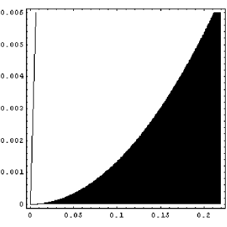
(a) $|\omega|\ vs.\ \Delta t(\Gamma^{-1})$; for $\Omega=0$

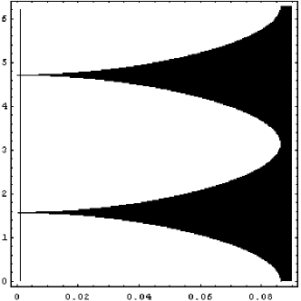
(b) $\Omega\ vs.\ \Delta t(\Gamma^{-1})$; for $|\omega|=0.001$

Figure 6.4: Level curves for $\frac{1}{\Gamma}|dA_{sl}/d\Delta t|=0.1$, the white area represents the points where $\frac{1}{\Gamma}|dA_{sl}/d\Delta t|>0.1$, and hence the time variation is (expected to be) experimentally detectable. Notice the tiny dark line on the left of each graph which represents the peak of the asymmetry, where of course the derivative also goes to zero. Fig. (a) plots $|\omega|\ vs.\ \Delta t$ for a fixed $\Omega=0$, observe that although to see the peak in $A_{sl}$ it is required a very high $\Delta t$-resolution, the region where the time variation is detectable might be more accessible experimentally. Fig. (b) plots the phase $\Omega\ vs.\ \Delta t$ for a fixed value of $|\omega|=0.001$, note that disregarding the values of the phase around $\pi/2$ and $3\pi/2$, the measurable region (white) is quite favoured in $\Delta t$.

Present limits on $\omega$ using existing data

Although the best region where to see the effects of $\omega$ is at small $\Delta t$, the existing data on the $A_{sl}$ asymmetry has not been taken in that region, but instead at $\Delta t\gtrsim 0.8\frac{1}{\Gamma}$ [36, 37] (see Eq. (4.11)). In fact, since in these experiments at last the $A_{sl}$ would be fitted to a constant, the small $\Delta t$ region was discarded to avoid the complications which come from the experimental background. On the other hand, we have shown in this work that to see the pronounced possible effects of $\omega$ it is mandatory to explore the small $\Delta t$ region. In any case, this existing data could be used to put limits on $\omega$, since its existence would produce a shift in the $\Delta t\sim 1/\Gamma$ region, as shown in Eq. (6.21).

We point out here that putting limits to $\omega$ using the available fit of $A_{sl}$ to a constant is not a direct constraint on $\omega$, but rather indirect. It is clear that a direct constrain on $\omega$ should be done using the original complete experimental data and fitting it to the expression $A_{sl}(\omega,\Delta t)$ that comes from constructing the asymmetry using Eq. (6.15) with its time dependence.

In order to find indirectly the allowed values for $\omega$ using the existing measurements of $A_{sl}$ we proceed as follows. Using Eq. (6.15) we compute the asymmetry as a function of $\omega$, and we allow $\epsilon$ to vary in its Standard Model expectation range [32],

$$\left|\frac{4Re(\epsilon)}{1+|\epsilon|^{2}}\right|={\cal O}\left(\frac{m_{c}^{2}}{m_{t}^{2}}\sin(2\beta)\right)\lesssim 0.001.$$ (6.23)

The values of $\omega$ which are within the $95\%$ C.L. are those such that $A_{sl}(\Delta t,\omega)$ is within the two standard deviation of the measured value of the asymmetry,

$$A_{sl}^{exp}=0.0019\pm 0.0105.$$ (6.24)

(This value comes from the equally weighted average of Refs. [36, 37], see Eq. (4.11).) Of course that we need to define what is ’within’, since $A_{sl}(\Delta t,\omega)$ is time-dependent, whereas $A_{sl}^{exp}$ is constant and, besides, the density of experimental events, $\rho(\Delta t)$, is highly $\Delta t$-dependent. With this purpose, we define a density-weighted average difference between the experimental and $\omega$-theoretical asymmetries as

$$\Delta A_{sl}(\omega) = \frac{\int_{\Delta t_{1}}^{\Delta t_{2}}\rho(\Delta t)(A_{sl}(\Delta t,\omega)-A_{sl}^{exp})\,d\Delta t}{\int_{\Delta t_{1}}^{\Delta t_{2}}\rho(\Delta t)\,d\Delta t},$$ (6.25)

where $(\Delta t_{1},\Delta t_{2})=(0.8\frac{1}{\Gamma},8\frac{1}{\Gamma})$ is the range of times where the measurements have been performed, and the density of events is

$$\rho(\Delta t) = e^{-\Gamma\Delta t}(1-\cos(\Delta m\Delta t)).$$ (6.26)

Where in the density function $\rho(\Delta t)$ we have approximated $\Delta\Gamma\approx\omega\approx 0$ since at this point they constitute second order contributions. From the definition of weighted-average-difference in Eq. (6.25) we obtain the $95\%$ C.L. allowed values for $\omega$ as those that furnish

$$|\Delta A_{sl}(\omega)|\leq 2\sigma=0.0210.$$ (6.27)

The fulfilment of this equation, neglecting quadratic contributions in $\omega$, gives the final result:

$$-0.0084\leq Re(\omega)\leq 0.0100\qquad~{}\quad 95\%\mbox{C.L.}$$ (6.28)

Where the values of $\epsilon$ used to define the upper and lower limits correspond in each case to those in Eq. (6.23) which extend the most the allowed range for $\omega$. These are the first known limits on $\omega$.

It is interesting to notice that if this same calculation is performed approximating $A_{sl}(\Delta t,\omega)$ by its value at the typical time $\Delta t=1/\Gamma$, see Eq. (6.21), we obtain the approximated limits $-0.0059\lesssim Re(\omega)\lesssim 0.0070$ which is a good –and simpler– estimation compared to the exact value in Eq. (6.28).

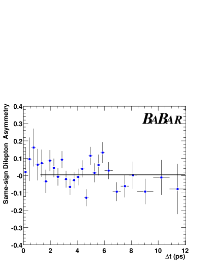
(a) Babar, $\Delta t=\frac{"\Delta t(ps)"}{1.53ps}\Gamma^{-1}$

(b) Belle, $\Delta t=\frac{|\Delta z|}{0.0186cm}\Gamma^{-1}$

Figure 6.5: Reproduction of the experimental results for the $A_{sl}$ asymmetry by Babar [36] and Belle [37] collaborations. The points for the fitting (the constant solid line in each figure) are taken for $\Delta t>0.8\Gamma^{-1}$. As it is seen in the figures, the time independence of the $A_{sl}$ asymmetry, as well as its fitting, have not arrived yet to a definite conclusion. Notice also that the $\omega$-effect predicts a second peak at $\Delta t\approx 8.2\Gamma^{-1}$ ($\Delta z\approx 0.15\,cm,\ \Delta t\approx 12.4\,ps$) which the data cannot discard; see Fig. (6.3b) and text therein.

To close this discussion we find convenient to reproduce here some experimental results for the $A_{sl}$ asymmetry. In Fig. (6.5) we reproduce Babar and Belle’s results on the asymmetry. As it can be seen, the fitting to a constant is not conclusive yet: further measurements are required to give a more precise answer on the $\omega$-effect.

Statistical analysis

Figure 6.6: Figure of merit for measuring the equal-sign dilepton charge asymmetry; from bottom to top $\omega=0$ (solid line), $\omega=0.0003$ (long-dashed), $\omega=0.0006$ (medium-dashed) and $\omega=0.001$ (short-dashed). Observe how the peak in the $A_{sl}$ asymmetry for $\omega\neq 0$ is reflected here as a growth and a $\Delta t$-shift towards the origin of the maximum. This shows that as $\omega\neq 0$, its effects are found to be in the small $\Delta t$ region and at the same time this region becomes statistically easier to explore. The figure of merit proves the high sensibility that exists in the asymmetry to measure $\omega$.

To complete the analysis of the equal-sign dilepton charge asymmetry, we study how the statistic requirements are modified due to the presence of $\omega$. From the statistical analysis point of view, the relevant quantity to observe an asymmetry as a function of $\Delta t$ is the figure of merit, i.e. $I(X,X^{\prime},\Delta t)\cdot(A_{sl}(\Delta t))^{2}$. As it is well known, the minimum number of events needed to measure the asymmetry is proportional to its inverse. The figure of merit is plotted in Fig. (6.6) for different values of $\omega$. In this plot one may see the high sensibility on $\omega$: as $|Re(\omega)|$ grows, the maximum also grows and it is shifted towards smaller $\Delta t$’s. This behaviour gives to the asymmetry a high sensibility on $\omega$: as was explained above, the effects of $\omega$ are found enhanced in the small $\Delta t$ region, whereas the figure of merit tells us that as $|Re(\omega)|$ grows, the exploration of this region becomes more effective.

Chapter 7 Conclusions and outlook

In this work we have analyzed and studied the effects of the violation of the symmetries T and CP, and the possible violation of CPT, in the correlated B-meson system. The analysis has been performed from two different points of view. In Chapter 5 we have analyzed how the mixing and decay observables corresponding to correlated CP and flavour decays depend on these three discrete symmetries. In Chapter 6, instead, we have studied solely the effects of a novel kind of CPT violation whose effects would arise in the initial state of the B-factories through the no longer indistinguishability of $B^{0}$ and $\bar{B^{0}}$; producing, hence, a variety of modification in the usual B-physics observables. We analyze separately the conclusions of these two different sets of results.

In Chapter 5 we have shown rigorously how to place a CP-tag. Although there is no $CP_{\Theta\Theta^{\prime}}$ operator which leaves invariant the whole Hamiltonian including the charged current term, we have shown how a specific choice of $\Theta\mbox{ and }\Theta^{\prime}$ determines a CP_A operator which commutes with a chosen piece of this charged current term, under a $O(\lambda^{4})$ approximation. This piece is the only part of the charged currents involved in the direct (with no mixing) decay of the $B$ meson into $J/\psi K_{S,L}$: the Golden Plate decay. With this determination, the initial state coming from the $\Upsilon(4S)\to B^{0}\bar{B^{0}}$ decay is written in terms of the CP_A eigenstates, and therefore a decay of the first $B$ meson into a Golden Plate CP+ state places a CP${}_{A}-$ tag in the second $B$ meson. And vice-versa.

Having obtained a CP_A operator which commutes with the piece of Hamiltonian involved in the direct Golden Plate decay of the $B$ meson, gives us a powerful tool which makes the analysis of the adequate correlated decays to get reduced to the $B$-mixing. In fact, with this CP-tag and the well-known flavour tag coming from the flavour specific channels, we can obtain all possible intensities relating final CP-eigenstate and flavour-specific decays by studying the one-meson-transition in the $\Delta t$-mixing. The right choice of the $B$ basis at the beginning and at the end of the mixing, namely $\{B_{\pm A}\}$ or $\{B^{0},\,CP_{A}B^{0}\}$ depending on the decay, reduces the calculation to the mixing of the $B$ meson. Within any of these basis, we have proved that no phase ambiguities are found and therefore the $\epsilon$ parameter is rephasing-invariant.

We have completed the analysis of correlated neutral $B$-meson decays into flavour and CP eigenstates in terms of single $B$-meson transitions in the time interval $\Delta t$ between both decays. The action of the discrete symmetries CP, T and CPT is thus described in terms of initial and final $B$-states. In Section 5.5 a variety of new observables have been proposed to show the consistency of the entire picture, as well as to explore the possible existence of physics beyond the Standard Model . For instance, assuming CPT invariance the correlated CP-forbidden $(J/\psi K_{S},\,J/\psi K_{S})$ and $(J/\psi K_{L},\,J/\psi K_{L})$ decays shall have equal intensities. As apparent from their CP-forbidden character, each of them comes out to be proportional to $\sin^{2}(2\beta)$, with the same $\Delta t$ dependence as the $(\ell^{+},\,\ell^{+})$ correlated decay (see Eq. (5.63)). Using the advantages of the CP-tag, we have also proposed observables for observing direct T-violation (see Eq. (5.48)). At the same time we have remarked the difference between the T-operation and the $\Delta t$-operation –consisting in the exchange in the order of appearance of the decay products– when $\Delta\Gamma\neq 0$. We have also computed the usual observable which measures $\sin(2\beta)$ through the CP asymmetry Eq. (5.40).

The genuine symmetries studied have also been combined with the $\Delta t$ operation. Although $\Delta t$-exchange and T-reversal lead to different processes, they must have equal intensities in the limit $\Delta\Gamma=0$ if CPT is assumed. We then suggest the comparison of processes connected by CP$\Delta t$-operation in order to extract linear terms in $\Delta\Gamma$, as explicitly seen in Eqs. (5.58) and (5.62). In the $B_{d}$-system, these CP$\Delta t$-asymmetries are expected to be small. One could envisage the use of these observables to determine $\Delta\Gamma_{s}$ for the $B_{s}$-system, with expected larger width-difference, by means of the $B$-factories operating at $\Upsilon(5S)$.

It is worth to note that in studying the double CP decays we have also found that, as in the case of CP-semileptonic decays, the sign of $\cos(2\beta)$ remains either hidden or accompanied by the sign of $\Delta\Gamma$.

In Chapter 6 we have studied the consequences that CPT violation could have on the initial $B^{0}\bar{B^{0}}$ entangled-state in the B-factories. The loss of indistinguishability of particle-antiparticle yields to the relaxation of Bose-statistics requirement, which is characterized by the complex parameter $\omega$ (Eq. (6.2)). We have shown that this $\omega$-effect would bring out important conceptual and measurable modifications in the correlated B-meson system.

The most important conceptual change, the demise of flavour tagging, comes out from the loss of the definite anti-symmetry in the initial state. In fact, if $\omega\neq 0$ then the time evolution of the initial state will project a component on the $|B^{0}B^{0}\rangle$ and $|\bar{B^{0}}\bar{B^{0}}\rangle$ states, which are clearly forbidden in the $\omega=0$ case. The appearance of these forbidden states produces the demise of the flavour tag: a flavour-specific $B^{0}$ decay on one side allows a presence (proportional to $\omega$) of the same $B^{0}$ meson on the wave function in the other side at the same time, and viceversa. We show that this effect would be measurable through the CP asymmetry consisting of the $\Delta t=0$ same sign semi-leptonic intensities, $A_{CP}(t)$ and ${\cal A}_{CP}$ (Eq. (6.9)). Notice, however, that although conceptually appealing, this observable requires a $|\omega|^{2}$ precision in the measurement of the intensities.

In order to look for an observable linear in $\omega$ we have analyzed the $\Delta t$-dependence of the equal-sign semi-leptonic correlated decays. Here the interference terms give rise to the expected linear in $\omega$ modifications. We have computed the equal-sign dilepton events in correlated B-decays, $I(\ell^{\pm},\ell^{\pm},\Delta t)$ (see Eq. (6.15) and Fig. (6.1)). We have found corrections linear in $Re(\omega)$ with opposite behaviour depending on the sign of the leptons, and therefore pointing to their asymmetry as an optimal observable where to look for traces of $\omega$.

The equal-sign dilepton charge asymmetry, $A_{sl}$, has been already studied and measured for the case $\omega=0$, where its behaviour is known to be constant and proportional to the CP violating parameter $Re(\epsilon)$. The computation of the $A_{sl}$ asymmetry for $\omega\neq 0$, on the other hand, shows a strong time-dependence in the small $\Delta t$ region (where it has not been measured yet), and a quasi time-independent shift in the later (measured) $\Delta t\sim\Gamma^{-1}$ region. At small $\Delta t\sim|\omega|\Gamma^{-1}$ we find a pronounced peak, whose tail could be detectable for later $\Delta t$’s (see Figs. (6.2-6.4).

Current experiments have been performed in the $\Delta t\gtrsim\Gamma^{-1}$ region, and are consistent with a possible existence of $\omega\neq 0$. Moreover, the difference between the Standard Model expectation for $Re(\epsilon)$ and the measured two-standard-deviation allowed range for the equal-sign dilepton charge asymmetry, allows us to compute indirectly the current limits on the value of $Re(\omega)$ at a $95\%$ confidence limit,

$$-0.084\leq Re(\omega)\leq 0.0100\qquad 95\%\mbox{ C.L.}$$ (7.1)

These are the first known limits on $\omega$. This limit can be improved by the progress in the experimental measure of the asymmetry or, much more definitive, by the exploration of the small-$\Delta t$ region. This, of course, requires a new treatment of the background, which complicates the measure of the flavour-specific channels in that region.

From the statistics point of view, we have shown using the figure of merit that as $\omega\neq 0$ its greater effects are found in the small $\Delta t$-region and at the same time this region becomes easier to explore. Hence, the experimental probe of the small-$\Delta t$ region is crucial for determining the possible existence of CPT violation through distinguishability of particle-antiparticle.

The results of this thesis advocate and endorse the experimentalists to explore the low-$\Delta t$ region in the equal-sign dilepton events.

The implications due to a non-vanishing value of $\omega$ are not only visible in the dilepton channels. We plan to explore this effect in the correlated (flavour,CP) and (CP,flavour) decays, as demanded for the Golden Plate channels.

Chapter 7 Conclusiones y perspectivas [español]

En este trabajo hemos analizado y estudiado los efectos de la violación de las simetrías T y CP, y la posible violación de CPT en el sistema de mesones B correlacionados. El análisis ha sido realizado desde dos puntos de vista diferentes. En el Capítulo 5 hemos analizado cómo observables de mixing y decaimiento, correspondientes a decaimeintos correlacionados de sabor y CP, dependen de estas tres simetrías discretas. En el Capítulo 6, en cambio, hemos estudiado sólamente los efectos de una flamante clase de violación de CPT cuyos efectos surgirían en el estado inicial de las fábricas de B, a través de la pérdida de indistinguibilidad entre $B^{0}$ y $\bar{B^{0}}$; produciendo entonces una variedad de modificaciones en los observables usuales de la física de B’s. Analizamos separadamente las conclusiones de estos dos conjuntos de resultados diferentes.

En el Capítulo 5 demostramos rigurosamente cómo colocar un rótulo de CP (CP-tag). Aunque no exista un operador $CP_{\Theta\Theta^{\prime}}$ que deje invariante todo el Hamiltoniano incluyendo la parte de corrientes cargadas, hemos mostrado cómo una elección específica de $\Theta$ y $\Theta^{\prime}$ determina el operador CP_A que conmuta con una pieza seleccionada de éste término de corrientes cargadas, en la aproximación de ${\cal O}(\lambda^{4})$. Esta pieza es la única parte de las corrientes cargadas que está involucrada en el decaimiento directo (sin mixing) del meson B en $J/\psi K_{S,L}$: el decaimiento Golden Plate. Con esta determinación, el estado inicial proveniente del decaimiento $\Upsilon(4S)\to B^{0}\bar{B^{0}}$ es escrito en término de los autoestados de CP_A, y entonces un primer decaimiento a un Golden Plate CP+ coloca un rótulo CP${}_{A}-$ en el segundo mesón en vuelo. Y viceversa.

Haber obtenido un operador CP_A que conmuta con la pieza de Hamiltoniano involucrada en el decaimiento Golden Plate, nos ofrece una poderosa herramienta que hace que el análisis de los decaimientos correlacionados adecuados quede reducido al mixing de los B’s. En efecto, con el rótulo por CP y el bien conocido rótulo por sabor que proviene de los canales de sabor-específico, podemos obtener todas las posibles intensidades que relacionan decaimientos finales de autoestados de CP y de sabor-específico, estudiando la transición de un mesón en el mixing durante $\Delta t$. La elección correcta de la base de B’s al comienzo y al final del mixing, llámese $\{B_{\pm A}\}$ y $\{B^{0},CP_{A}B^{0}\}$ según el decaimiento, reduce todo el cálculo al mixing de un único mesón B. En cualquiera de estas bases hemos probado que no existe ambigüedad en las fases, luego $\epsilon$ es un parámetro invariante de fase.

Hemos completado el análisis de los decaimientos de mesones neutros B correlacionados en canales de sabor y de autoestados de CP en término de transiciones de un único mesón B en el intervalo de tiempo $\Delta t$ entre los dos decaimientos. La acción de las simetrías discretas CP, T y CPT es entonces descrita en término de estados iniciales y finales de mesones B. En la Sección 5.5 una variedad de nuevos observables han sido propuestos para mostrar la consistencia del modelo, así como explorar la posible existencia de física mas allá del Modelo Estándar. Por ejemplo, suponiendo invarianza CPT, los decaimientos correlacionados CP-prohibidos $(J/\psi K_{S},J/\psi K_{S})$ y $(J/\psi K_{L},J/\psi K_{L})$ deben tener la misma intensidad. Tal como es aparente de su caracter CP-prohibido, cada uno de ellos resulta proporcional a $\sin^{2}(2\beta)$, con la misma dependencia en $\Delta t$ que el decaimiento $(\ell^{+},\ \ell^{+})$ (ver Ec. (5.63)). Usando las ventajas del rótulo por CP, hemos también propuesto observables para medir violación directa de T (ver Ec. (5.48)). A la vez hemos remarcado la diferencia que existe entre las operaciones T y $\Delta t$ –que consiste en intercambiar el orden de los decaimientos– cuando $\Delta\Gamma\neq 0$. También hemos construido el observable usual para la medición de $\sin(2\beta)$, la asimetría CP en Ec. (5.40).

Las simetrías genuinas estudiadas también han sido combinadas con la operación $\Delta t$. Aunque el intercambio-$\Delta t$ y la operación de inversión temporal T conducen a diferentes procesos, estos deben tener la misma intensidad en el límite $\Delta\Gamma=0$ si CPT es válido. Teniendo en cuenta esto, sugerimos la comparación de procesos conectados por la operación CP$\Delta t$, para así extraer términos lineales en $\Delta\Gamma$, como se ve explícitamente en las Ecs. (5.58) y (5.62). En el sistema $B_{d}$ estas asimetrías CP$\Delta t$ se esperan que sean pequeñas. Sin embargo uno puede prever el uso de estos observables para determinar $\Delta\Gamma_{s}$ en el sistema $B_{s}$, donde se esperan mayores anchuras, usando las fábricas de B operando en la resonancia del $\Upsilon(5S)$.

Es conveniente notar que al estudiar los decaimientos doble-CP hemos nuevamente hallado, como es en el caso de los decaimientos CP-semileptónicos, que el signo de $\cos(2\beta)$ sigue u oculto, o acompañado por el signo de $\Delta\Gamma$.

En el Capítulo 6 hemos estudiado las consecuencias que podría tener violación de CPT sobre el estado inicial de los mesones $B^{0}\bar{B^{0}}$ correlacionados en las fábricas de B. La pérdida de indistinguibilidad entre partícula y antipartícula conduce al relajamiento del requisito de estadística de Bose, caracterizado por el parámetro $\omega$ (Ec. (6.2)). Hemos mostrado que este efecto-$\omega$ podría implicar importantes modificaciones conceptuales y medibles en el sistema de mesones B correlacionados.

El cambio conceptual más importante, el ’fin’ del rótulo por sabor, se debe a la pérdida de la anti-simetría definida en el estado inicial. En efecto, si $\omega\neq 0$ entonces la evolución temporal del estado inicial tendrá una proyección sobre los estados $|B^{0}B^{0}\rangle$ y $|\bar{B^{0}}\bar{B^{0}}\rangle$ no nula, la cual está claramente prohibida en el caso de $\omega=0$. La aparición de estos estados prohibidos produce el ’fin’ del rótulo por sabor: un decaimiento de sabor-específico $B^{0}$ en un lado permite una presencia (proporcional a $\omega$) del mismo mesón $B^{0}$ en el otro lado al mismo tiempo, y viceversa. Hemos demostrado que este efecto sería medible a través de una asimetría CP que consista de las intensidades dileptónicas de mismo signo con $\Delta t=0$, $A_{CP}(t)$ y ${\cal A}_{CP}$ (Eq. (6.9)). Nótese, de todos modos, que aunque conceptualmente importante, este observable requiere una precisión de $|\omega|^{2}$ en la medición de las intensidades.

Con el objeto de buscar un observable lineal en $\omega$ hemos analizado la dependencia en $\Delta t$ de los decaimientos correlacionados semileptónicos de mismo signo. Aquí los términos de interferencia dan lugar a las buscadas modificaciones lineales en $\omega$. Hemos computado los eventos de dos leptones del mismo signo en los decaimientos correlacionados de mesones B, $I(\ell^{\pm},\ell^{\pm},\Delta t)$ (ver Ec. (6.15) y Fig. (6.1)). Hemos hallado correcciones lineales en $\omega$ con comportamientos opuestos dependiendo en los signos de los leptones, apuntando de este modo a su asimetría como un óptimo observable donde buscar rastros del efecto-$\omega$.

La asimetría de carga de eventos dileptónicos del mismo signo, $A_{sl}$, ha sido ya estudiada y medida para el caso $\omega=0$, donde su comportamiento se predice constante y proporcional al parámetro de violación de CP $Re(\epsilon)$. El cálculo de la asimetría $A_{sl}$ con $\omega\neq 0$, sin embargo, muestra una fuerte dependencia temporal en la región de $\Delta t$ pequeños (donde no ha sido medida aun), y un corrimiento cuasi-independiente del tiempo para tiempos posteriores $\Delta t\sim\Gamma^{-1}$ (donde si se ha medido). Para pequeños $\Delta t\sim|\omega|\Gamma^{-1}$ hallamos un pico pronunciado, cuya cola podría ser detectable en $\Delta t$ posteriores (ver Figs. (6.2-6.4)).

Los experimentos actuales han sido realizados en la región $\Delta t\gtrsim\Gamma^{-1}$, y son consistentes con la posible existencia de $\omega\neq 0$. Es más, la diferencia entre el valor que predice el Modelo Estándar para $Re(\epsilon)$ y el rango permitido por las dos desviaciones estándares de la medición de la asimetría $A_{sl}$, nos permite establecer indirectamente los límites actuales para el valor de $Re(\omega)$ a un nivel de $95\%$ de límite de confianza,

$$-0.084\leq Re(\omega)\leq 0.0100\qquad 95\%\mbox{ L.C.}$$ (7.1)

Estos son los primeros límites conocidos para $\omega$. Este límite puede ser mejorado a través de una mejor y más precisa medición de la asimetría o, en forma más definitiva, explorando la región de $\Delta t$ pequeños. Esto, claro está, requiere un nuevo tratamiento del fondo, ya que éste complica la medición de canales específicos de sabor en esa región.

Desde el punto de vista de la estadística, hemos demostrado usando la figura de mérito que si $\omega\neq 0$ entonces sus efectos se hallan en la región de $\Delta t$’s pequeños y a la misma vez esta región es más fácil de explorar. Luego, el análisis experimental de la región de pequeños $\Delta t$’s es crucial para determinar la posible existencia de violación de CPT a través de distinguibilidad de partícula y antipartícula.

Los resultados de esta tesis ponderan y respaldan a los experimentales a explorar la región de pequeños $\Delta t^{\prime}s$ en los eventos dileptónicos del mismo signo.

Las implicaciones de un posible $\omega$ diferente de cero son visibles no sólo en los canales dileptónicos. Nuestro plan es explorar este efecto en los decaimientos correlacionados (sabor,CP) y (CP,sabor), para observar las correcciones que produciría en los canales Golden Plate.

AGRADECIMIENTOS

Allá, por los comienzos de 2001, habrían pasado no más de algunas semanas de mi licenciatura, no tenía siquiera un proyecto de qué hacer en el futuro, pero ya me encontraba ofreciendo (¿canjeando?) agradecimientos para mi tesis doctoral. Hoy, 15 de noviembre de 2005, como todo hombre que se digna de sí mismo, me debo a mi Palabra.

• Gracias a la Universidad de Valencia por el apoyo económico durante estos cuatro años a través de la Beca Cinc Segles. Gracias a Fundación Antorchas y Fundación Kónex por haber depósitado su confianza en mí y, en los tiempos más duros de Argentina, haberme adjudicado sendas becas para que pudiese venir a realizar mi doctorado en la Universidad de Valencia. Gracias a Sofía Rawson y a Luis Ovsejevich por su grandeza y dignidad, sus desinteresados respaldo y apoyo, y por su confianza en mí. Gracias a los Departamentos de Física de la Universidad de Valencia y de la Universita Degli Studi di Roma La Sapienza, cuyos recursos fueron indispensables para realizar los trabajos contenidos en esta tesis.

• Debo agradecer fuerte y enormemente a Pepe Bernabéu su sabia guía y ayuda, y su constante respaldo y apoyo durante estos cuatro años, así como también le agradezco por haberme aceptado para realizar este doctorado bajo su supervisión.

  Gracias a Joannis Papavassiliou por su ayuda y guía, también a Miguel Nebot y Nick Mavromatos por las, finalmente ricas, tertulias e intercambio de ideas.

  Gracias a Alejandro Szynkman, Luis Epele, Carlos García-Canal y Daniel Gómez-Dumm por su apoyo para trabajar con ellos durante mi estancia en la Universidad de La Plata.

  Gracias a C. García-Canal, N. Mavromatos y L. Silvestrini por sus útiles comentarios y aportes en la lectura del manuscrito.

  Gracias a Vicente Vento y a Miguel Angel Governa, quienes llevarán aquí el rótulo de partícipes necesarios.

• Vaya un gracias mayúsculo para Los Viejos, Ingrid y Hugo, por su constante apoyo en todas y cada una de las situaciones que me ha tocado en suerte vivir. Otro gracias especial a Agustín, por su interminable apoyo y camaradería.

  Gracias a Carla, por su fiel apoyo, por su compañía, por su colaboración. Y también gracias, por su eterna comprensión.

  Gracias a los gomías, Federico y Martín, gracias a la Eli; gracias a Pablo Eggarter; gracias a Carmen y a Jorgelina, gracias a su familia; gracias a Mirta y familia; gracias a Gonzalo, camarada de mar agitado; gracias a Asunción por su implacable ayuda y apoyo, y también gracias a Alicia, Cristina y Pilar; gracias a Ada, por su cariño y colaboración; gracias a Marek y Minou, gracias a la familia Kaczorowski; gracias a Ale Szynkman, el sensei del Sur; gracias a Diego Mazzitelli; gracias al Sr. Jose Fernando Benítez-Villena, al Sr. Jorge Cabero, al Sr. Fabio Lanci, al Sr. Fausto Troilo y al Sr. Massimo Milano; gracias a Carlo, Adriana y Sergio, gracias a la familia Zilli en toda su extensión; gracias a Inma, gracias a Natalia, Angel y a la familia Basante-López; gracias a Sara; gracias a las vecinas del primero, las Navarro-Cayuela; gracias a Cristian Batista, a Rolando Somma, a Gerardo Ortíz; gracias a Raquel Antelo; gracias a mis dos Yamahitas, compañeras de aventuras; gracias al Bar Zakate y los sólitos compañeros que allí paran, Jaqueline, Bea, Julia, Jorge, Claudia, etc.; Gracias a Julieta Ugartemendía, gracias a sus vecinos venezolanos y compañeras de piso; gracias a Joannis, Catalina, Teresa, David y a El Limbo; gracias a Cinthia; gracias a Carmen y a Elena; gracias a Caro y Guilleaume, gracias a Jul Bidu; gracias a Andrea Trenes; gracias a Carolina Toledo; gracias a Miguel Socolovsky, espíritu de la revolución; gracias a Warhol y a la extensión de caracteres que allí habitan, gracias a Diego, Gato, Juancho y sus compañeras; gracias a Susana Asencio y a Sakura, develadoras de horizontes; gracias al Gordo Tato y al Antro por esos infinitos asados; gracias a la Tierra, por habernos dado la música; gracias a la vida, que me ha dado tanto.

Bibliography

- [1] J. H. Christenson, J. W. Cronin, V. L. Fitch and R. Turlay, Phys. Rev. Lett. 13 (1964) 138.
- [2] M. Kobayashi and T. Maskawa, Prog. Theor. Phys. 49, 652 (1973).
- [3] S. Weinberg, Phys. Rev. Lett. 19, 1264 (1967).
- [4] N. Cabibbo, Phys. Rev. Lett. 10, 531 (1963).
-
[5]
B. Aubert et al. [BABAR Collaboration],
Phys. Rev. Lett. 86, 2515 (2001)
[arXiv:hep-ex/0102030];
K. Abe et al. [Belle Collaboration], Phys. Rev. Lett. 87, 091802 (2001) [arXiv:hep-ex/0107061];
and all Babar’s and Belle’s production thereafter. - [6] A. D. Sakharov, Pisma Zh. Eksp. Teor. Fiz. 5, 32 (1967) [JETP Lett. 5, 24 (1967 SOPUA,34,392-393.1991 UFNAA,161,61-64.1991)].
-
[7]
In the Kaon system see
A. Alavi-Harati et al. [KTeV Collaboration], Phys. Rev. D 67, 012005 (2003) [Erratum-ibid. D 70, 079904 (2004)] [arXiv:hep-ex/0208007];
in the B mesons see Refs. [41][42] and
K. Ackerstaff et al. [OPAL Collaboration], Z. Phys. C 76, 401 (1997) [arXiv:hep-ex/9707009]. - [8] W. Pauli, Nuo. Cim., 6, 204 1957.
-
[9]
See Refs. [12][50] and
V. A. Kostelecky, Phys. Rev. D 64 (2001) 076001 [arXiv:hep-ph/0104120];
D. Colladay and V. A. Kostelecky, Phys. Lett. B 344, 259 (1995) [arXiv:hep-ph/9501372];
M. Kobayashi and A. I. Sanda, Phys. Rev. Lett. 69, 3139 (1992). - [10] J. Bernabeu, N. E. Mavromatos and J. Papavassiliou, Phys. Rev. Lett. 92, 131601 (2004) [arXiv:hep-ph/0310180].
- [11] S. Hashimoto et al., KEK-REPORT-2004-4, and references therein.
- [12] M. C. Banuls and J. Bernabeu, Phys. Lett. B 464, 117 (1999) [arXiv:hep-ph/9908353].
- [13] E. Alvarez, J. Bernabeu, N. E. Mavromatos, M. Nebot and J. Papavassiliou, Phys. Lett. B 607, 197 (2005) [arXiv:hep-ph/0410409].
-
[14]
Ref. [3] and
S. L. Glashow, Nucl. Phys. 22, 579 (1961);
A. Salam, ”Elementary Particle Theory”, Almqvist & Wiksell (1968). - [15] C. Jarlskog, ”CP-violation”, World Scientific (1989).
- [16] W. Grimus and M. N. Rebelo, Phys. Rept. 281, 239 (1997) [arXiv:hep-ph/9506272].
- [17] P. H. Frampton and C. Jarlskog, Phys. Lett. B 154, 421 (1985).
-
[18]
J. Bernabéu and P. Pascual, ”Electro-Weak Theory”, Univ. Aut. Barcelona, B-21399 (1981);
A. Pich, arXiv:hep-ph/9412274. -
[19]
L. L. Chau and W. Y. Keung,
Phys. Rev. Lett. 53, 1802 (1984);
F. J. Botella and L. L. Chau, Phys. Lett. B 168, 97 (1986);
H. Harari and M. Leurer, Phys. Lett. B 181, 123 (1986);
H. Fritzsch and J. Plankl, Phys. Rev. D 35, 1732 (1987). - [20] M. Schmidtler and K. R. Schubert, Z. Phys. C 53, 347 (1992).
- [21] A. J. Buras, M. E. Lautenbacher and G. Ostermaier, Phys. Rev. D 50, 3433 (1994) [arXiv:hep-ph/9403384].
- [22] L. Wolfenstein, Phys. Rev. Lett. 51, 1945 (1983).
- [23] J. Bernabeu, G. C. Branco and M. Gronau, Phys. Lett. B 169, 243 (1986).
- [24] C. Jarlskog, Phys. Rev. Lett. 55, 1039 (1985).
- [25] R. Aleksan, B. Kayser and D. London, Phys. Rev. Lett. 73, 18 (1994) [arXiv:hep-ph/9403341].
- [26] C. Jarlskog and R. Stora, Phys. Lett. B 208, 268 (1988).
- [27] G. D. Rochester and C. C. Butler, Nature 160, 855 (1947).
- [28] M. Gell-Mann and A. Pais, Phys. Rev. 97, 1387 (1955).
- [29] V. Weisskopf and E. P. Wigner, Z. Phys. 63, 54 (1930); for a more modern review, with the degenerated case already included, see Ref. [51]
- [30] J. P. Silva, Phys. Rev. D 62, 116008 (2000) [arXiv:hep-ph/0007075].
-
[31]
L. Alvarez-Gaume, C. Kounnas, S. Lola and P. Pavlopoulos,
Phys. Lett. B 458, 347 (1999)
[arXiv:hep-ph/9812326];
L. Alvarez-Gaume, C. Kounnas, S. Lola and P. Pavlopoulos [CPLEAR Collaboration], arXiv:hep-ph/9903458. - [32] S. Eidelman et al. [Particle Data Group], Phys. Lett. B 592, 1 (2004).
- [33] P. Raimondi, EPAC-2004-FRXBCH02 Presented at the 9th European Particle Accelerator Conference (EPAC 2004), Lucerne, Switzerland, 5-9 Jul 2004
- [34] For further reading on the subject see, for instance, A.D. Martin and T.D. Spearman, ”Elementary particle theory”, North-Holland Publishing Company (1970).
- [35] A. Angelopoulos et al. [CPLEAR Collaboration], Phys. Lett. B 444 (1998) 43.
- [36] B. Aubert et al. [BABAR Collaboration], Phys. Rev. Lett. 88 (2002) 231801 [arXiv:hep-ex/0202041].
- [37] E. Nakano et al. [Belle Collaboration], arXiv:hep-ex/0505017.
- [38] Y. Y. Keum and A. I. Sanda, Phys. Rev. D 67, 054009 (2003) [arXiv:hep-ph/0209014].
- [39] B. Aubert et al. [BaBar Collaboration], Phys. Rev. Lett. 93, 131801 (2004) [arXiv:hep-ex/0407057].
- [40] Y. Chao et al. [Belle Collaboration], Phys. Rev. Lett. 93 (2004) 191802 [arXiv:hep-ex/0408100].
- [41] B. Aubert et al. [BABAR Collaboration], Phys. Rev. Lett. 92 (2004) 181801 [arXiv:hep-ex/0311037].
- [42] N. C. Hastings et al. [Belle Collaboration], Phys. Rev. D 67 (2003) 052004 [arXiv:hep-ex/0212033].
- [43] E. Alvarez and J. Bernabeu, Phys. Lett. B 579, 79 (2004) [arXiv:hep-ph/0307093].
- [44] M. Gronau, O. F. Hernandez, D. London and J. L. Rosner, Phys. Rev. D 52, 6374 (1995) [arXiv:hep-ph/9504327], and references therein.
- [45] R. E. Shrock and S. B. Treiman, Phys. Rev. D 19, 2148 (1979).
- [46] G. Unal [NA48 Collaboration], arXiv:hep-ex/0209064.
- [47] See for instance Y. Nir and H. R. Quinn, Ann. Rev. Nucl. Part. Sci. 42, 211 (1992).
-
[48]
R. Itoh et al. [Belle Collaboration],
Phys. Rev. Lett. 95, 091601 (2005)
[arXiv:hep-ex/0504030];
B. Aubert et al. [BABAR Collaboration], Phys. Rev. D 71 (2005) 032005 [arXiv:hep-ex/0411016]. - [49] J. Bernabeu, M. C. Banuls and F. Martinez-Vidal, Talk given at International Europhysics Conference on High-Energy Physics (HEP 2001), Budapest, Hungary; arXiv:hep-ph/0111073.
-
[50]
M. C. Banuls and J. Bernabeu,
Nucl. Phys. B 590, 19 (2000)
[arXiv:hep-ph/0005323];
M. C. Banuls and J. Bernabeu, Phys. Lett. B 423 (1998) 151 [arXiv:hep-ph/9710348]. - [51] P.K. Kabir, ”The CP Puzzle”, Academic Press (1968).
- [52] J. Bernabeu, Nucl. Phys. Proc. Suppl. 120, 332 (2003) [arXiv:hep-ph/0302063].
- [53] H. J. Lipkin, Phys. Rev. 176 (1968) 1715.
-
[54]
H. J. Lipkin,
Phys. Lett. B 219 (1989) 474;
I. Dunietz, J. Hauser and J. L. Rosner, Phys. Rev. D 35, 2166 (1987);
J. Bernabeu, F. J. Botella and J. Roldan, Phys. Lett. B 211, 226 (1988);
- [55] L. Wolfenstein, Nucl. Phys. B 246, 45 (1984).
- [56] J. Bernabeu, N. E. Mavromatos, J. Papavassiliou and A. Waldron-Lauda, arXiv:hep-ph/0506025.
-
[57]
Different analysis of can be found
in
G. V. Dass and K. V. L. Sarma, Phys. Rev. D 54 (1996) 5880 [arXiv:hep-ph/9607274]; Eur. Phys. J. C 5, 283 (1998) [arXiv:hep-ph/9709249];
Z. z. Xing, Phys. Lett. B 450, 202 (1999) [arXiv:hep-ph/9810249];
L. Lavoura and J. P. Silva, Phys. Rev. D 60 (1999) 056003 [arXiv:hep-ph/9902348];
G. V. Dass, W. Grimus and L. Lavoura, JHEP 0102, 044 (2001) [arXiv:hep-ph/0012131];
K. R. S. Balaji, W. Horn and E. A. Paschos, Phys. Rev. D 68, 076004 (2003) [arXiv:hep-ph/0304008].