The rare decays $B\to K^{(*)}\bar{K}^{(*)}$ and R-parity violating supersymmetry

Abstract

We study the branching ratios, the direct $CP$ asymmetries in $B\to K^{(*)}\bar{K}^{(*)}$ decays and the polarization fractions of $B\to K^{*}\bar{K}^{*}$ decays by employing the QCD factorization in the minimal supersymmetric standard model with R-parity violation. We derive the new upper bounds on the relevant R-parity violating couplings from the latest experimental data of $B\to K^{(*)}\bar{K}^{(*)}$, and some of these constraints are stronger than the existing bounds. Using the constrained parameter spaces, we predict the R-parity violating effects on the other quantities in $B\to K^{(*)}\bar{K}^{(*)}$ decays which have not been measured yet. We find that the R-parity violating effects on the branching ratios and the direct $CP$ asymmetries could be large, nevertheless their effects on the longitudinal polarizations of $B\to K^{*}\bar{K}^{*}$ decays are small. Near future experiments can test these predictions and shrink the parameter spaces.

PACS Numbers: 12.60.Jv, 12.15.Mm, 12.38.Bx, 13.25.Hw

1 Introduction

The study of exclusive hadronic $B$-meson decays can provide not only an interesting avenue to understand the $CP$ violation and flavor mixing of the quark sector in the standard model (SM), but also powerful means to probe different new physics (NP) scenarios beyond the SM. Recent experimental measurements have shown that some $B$ decays to two light mesons deviated from the SM expectations, for example, the $\pi\pi,\pi K$ puzzle [1] and the polarization puzzle in $B\rightarrow VV$ decays [2]. Although these measurements represent quite a challenge for theory, the SM is in no way ruled out yet since there are many theoretical uncertainties in low energy QCD. However, it will be under considerable strain if the experimental data persist for a long time.

Among those NP models that survived electroweak (EW) data, one of the most respectable options is the R-parity violating (RPV) supersymmetry (SUSY). The possible appearance of the RPV couplings [3], which will violate the lepton and baryon number conservation, has gained full attention in searching for SUSY [4, 5]. The effect of the RPV SUSY on $B$ decays have been extensively investigated previously in the literatures [6, 7], and it has been proposed as a possible resolution to the polarization puzzle and the $\pi\pi,\pi K$ puzzle [8]. The pure penguin $B\to K^{(*)}\bar{K}^{(*)}$ decays are closely related with the puzzles which are inconsistent with the SM predictions, and therefore are very important for understanding the dynamics of nonleptonic two-body $B$ decays, which have been studied in Refs. [9]. If the RPV SUSY is the right model to resolve these puzzles, the same type of NP will affect $B\to K^{(*)}\bar{K}^{(*)}$ decays. In this work, we shall study the RPV SUSY effects in the $B\to K^{(*)}\bar{K}^{(*)}$ decays by using the QCD factorization (QCDF) approach [10] for hadronic dynamics. The $B\to K^{(*)}\bar{K}^{(*)}$ decays are all induced at the quark level by $b\to ds\bar{s}$ process, and they involve the same set of RPV coupling constants. Using the latest experimental data and the theoretical parameters, we obtain the new upper limits on the relevant RPV couplings. Then we use the constrained regions of parameters to examine the RPV effects on observations in the $B\to K^{(*)}\bar{K}^{(*)}$ decays which have not been measured yet.

The paper is arranged as follows. In Sec.2, we calculate the $CP$ averaged branching ratios, the direct $CP$ asymmetries of $B\to K^{(*)}\bar{K}^{(*)}$ and the polarization fractions in $B\to K^{*}\bar{K}^{*}$ decays, taking account of the RPV effects with the QCDF approach. In Sec.3, we tabulate the theoretical inputs in our numerical analysis. Section 4 deals with the numerical results. We display the constrained parameter spaces which satisfy all the experimental data, and then we use the constrained parameter spaces to predict the RPV effects on the other observable quantities, which have not been measured yet in $B\to K^{(*)}\bar{K}^{(*)}$ system. Section 5 contains our summary and conclusion.

2 The theoretical frame for $B\to K^{(*)}\bar{K}^{(*)}$decays

2.1 The decay amplitudes in the SM

In the SM, the low energy effective Hamiltonian for the $\Delta B=1$ transition at the scale $\mu$ is given by [11]

$$\mathcal{H}^{SM}_{eff} = \frac{G_{F}}{\sqrt{2}}\sum_{p=u,c}\lambda_{p}\Biggl{\{}C_{1}Q_{1}^{p}+C_{2}Q_{2}^{p}+\sum_{i=3}^{10}\Big{[}C_{i}Q_{i}+C_{7\gamma}Q_{7\gamma}+C_{8g}Q_{8g}\Big{]}\Biggl{\}}+h.c.,$$ (1)

here $\lambda_{p}=V_{pb}V_{pq}^{*}$ for $b\to q$ transition $(p\in\{u,c\},q\in\{d,s\})$ and the detailed definition of the operator base can be found in [11].

Using the weak effective Hamiltonian given by Eq.(1), we can now write the decay amplitudes for the general two-body hadronic $B\to M_{1}M_{2}$ decays as

$$\mathcal{A}^{SM}(B\to M_{1}M_{2}) = \left<M_{1}M_{2}|{\cal H}^{SM}_{eff}|B\right>$$ (2)

$$= \frac{G_{F}}{\sqrt{2}}\sum_{p}\sum_{i}\lambda_{p}C_{i}(\mu)\left<M_{1}M_{2}|Q_{i}(\mu)|B\right>.$$

The essential theoretical difficulty for obtaining the decay amplitude arises from the evaluation of hadronic matrix elements $\langle M_{1}M_{2}|Q_{i}(\mu)|B\rangle$. There are at least three approaches with different considerations to tackle the said difficulty: the naive factorization (NF) [12, 13], the perturbative QCD [14], and the QCDF [10]. The QCDF developed by Beneke, Buchalla, Neubert and Sachrajda is a powerful framework for studying charmless $B$ decays. We will employ the QCDF approach in this paper.

The QCDF [10] allows us to compute the nonfactorizable corrections to the hadronic matrix elements $\langle M_{1}M_{2}|O_{i}|B\rangle$ in the heavy quark limit. The decay amplitude has the form

$$\mathcal{A}^{SM}(B\to M_{1}M_{2})=\frac{G_{F}}{\sqrt{2}}\sum_{p}\sum_{i}\lambda_{p}\Biggl{\{}a^{p}_{i}\langle M_{2}|J_{2}|0\rangle\langle M_{1}|J_{1}|B\rangle+b^{p}_{i}\langle M_{1}M_{2}|J_{2}|0\rangle\langle 0|J_{1}|B\rangle\Biggl{\}},$$ (3)

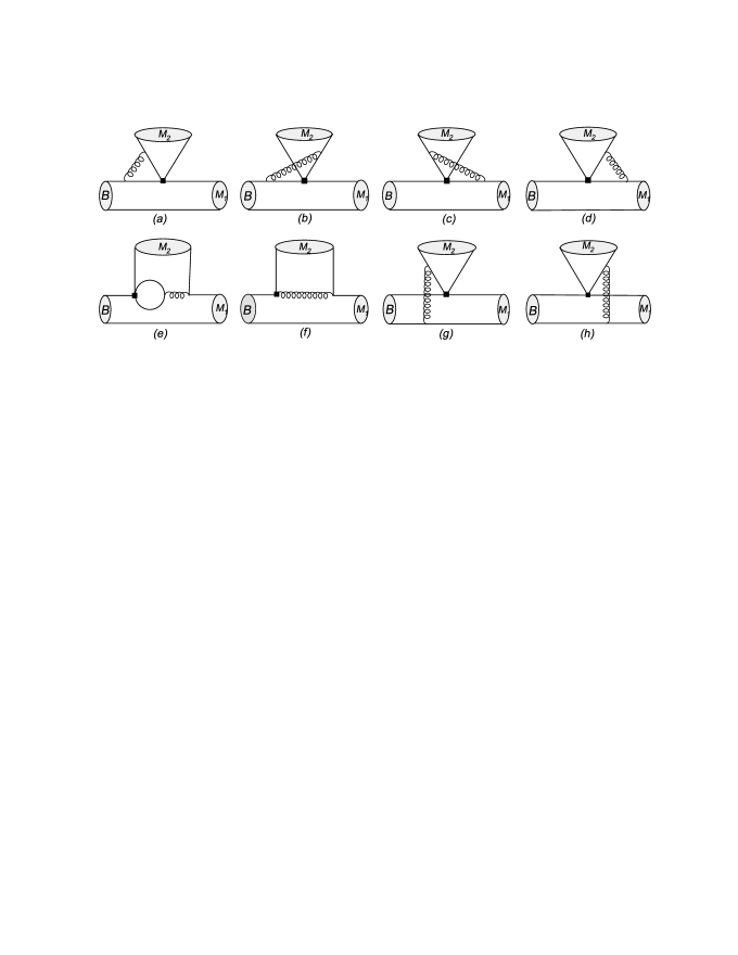
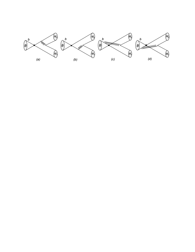
where the effective parameters $a_{i}^{p}$ including nonfactorizable corrections at order of $\alpha_{s}$. They are calculated from the vertex corrections, the hard spectator scattering, and the QCD penguin contributions, which are shown in Fig.1. The parameters $b_{i}^{p}$ are calculated from the weak annihilation contributions as shown in Fig.2.

Figure 1: The next to leading order nonfactorizable contributions to the coefficients $a^{p}_{i}$.

Figure 2: The weak annihilation contributions to the coefficients $b^{p}_{i}$.

Under the naive factorization (NF) approach, the factorized matrix element is given by

$$A_{M_{1}M_{2}}\equiv\langle M_{2}|(\bar{q}_{2}\gamma_{\mu}(1-\gamma_{5})q_{3})|0\rangle\langle M_{1}|(\bar{b}\gamma^{\mu}(1-\gamma_{5})q_{1})|B\rangle.$$ (4)

In term of the decay constant and form factors [15], $A_{M_{1}M_{2}}$ are expressed as

$$A_{M_{1}M_{2}}=\left\{\begin{array}[]{ll}if_{M_{2}}m_{B}^{2}F_{0}^{B\to M_{1}}(m^{2}_{M_{2}}),\hskip 142.26378pt\mbox{if $M_{1}=P,M_{2}=P$},\\ f_{M_{2}}m_{B}^{2}F_{0}^{B\to M_{1}}(m^{2}_{M_{2}}),\hskip 147.95424pt\mbox{if $M_{1}=P,~{}M_{2}=V$},\\ -f_{M_{2}}m_{B}^{2}A_{0}^{B\to M_{1}}(m^{2}_{M_{2}}),\hskip 139.41832pt\mbox{if $M_{1}=V,~{}M_{2}=P$},\\ -if_{M_{2}}m_{M_{2}}\biggl{[}(\varepsilon_{1}^{\ast}\cdot\varepsilon_{2}^{\ast})(m_{B}+m_{M_{1}})A_{1}^{B\to M_{1}}(m_{M_{2}}^{2})-(\varepsilon_{1}^{\ast}\cdot p_{B})(\varepsilon_{2}^{\ast}\cdot p_{B})\frac{2A_{2}^{B\to M_{1}}(m_{M_{2}}^{2})}{m_{B}+m_{M_{1}}}\biggr{.}\\ \hskip 56.9055pt\left.+i\epsilon_{\mu\nu\alpha\beta}\varepsilon_{2}^{\ast\mu}\varepsilon_{1}^{\ast\nu}p_{B}^{\alpha}p_{1}^{\beta}\frac{2V^{B\to M_{1}}(m^{2}_{M_{2}})}{m_{B}+m_{M_{1}}}\right],\hskip 34.14322pt\mbox{if $M_{1}=V,~{}M_{2}=V$},\end{array}\right.$$ (10)

where P(V) denote a pseudoscalar(vector) meson, $p_{B}(m_{B})$ is the four-momentum(mass) of the $B$ meson, $m_{M_{i}}$ is the masses of the $M_{i}$ mesons, and $\varepsilon_{i}^{\ast}$ is the polarization vector of the vector mesons $M_{i}$.

Following Beneke and Neubert [16], coefficients $a_{i}^{p}$ can be split into two parts: $a_{i}^{p}=a_{i,I}^{p}+a_{i,II}^{p}$. The first part contains the NF contribution and the sum of nonfactorizable vertex and penguin corrections, while the second one arises from the hard spectator scattering. The coefficients read [16]

$$a_{1,I}=C_{1}+\frac{C_{2}}{N_{C}}\left[1+\frac{C_{F}\alpha_{s}}{4\pi}V_{M_{2}}\right],\qquad\qquad\qquad\qquad a_{1,II}=\frac{C_{2}}{N_{C}}\frac{C_{F}\alpha_{s}}{4\pi}H_{M_{1}M_{2}},$$

$$a_{2,I}=C_{2}+\frac{C_{1}}{N_{C}}\left[1+\frac{C_{F}\alpha_{s}}{4\pi}V_{M_{2}}\right],\qquad\qquad\qquad\qquad a_{2,II}=\frac{C_{1}}{N_{C}}\frac{C_{F}\alpha_{s}}{4\pi}H_{M_{1}M_{2}},$$

$$a_{3,I}=C_{3}+\frac{C_{4}}{N_{C}}\left[1+\frac{C_{F}\alpha_{s}}{4\pi}V_{M_{2}}\right],\qquad\qquad\qquad\qquad a_{3,II}=\frac{C_{4}}{N_{C}}\frac{C_{F}\alpha_{s}}{4\pi}H_{M_{1}M_{2}},$$

$$a_{4,I}^{p}=C_{4}+\frac{C_{3}}{N_{C}}\left[1+\frac{C_{F}\alpha_{s}}{4\pi}V_{M_{2}}\right]+\frac{C_{F}\alpha_{s}}{4\pi}\frac{P^{p}_{M_{2},2}}{N_{C}},\qquad\qquad a_{4,II}=\frac{C_{3}}{N_{C}}\frac{C_{F}\alpha_{s}}{4\pi}H_{M_{1}M_{2}},$$

$$a_{5,I}=C_{5}+\frac{C_{6}}{N_{C}}\left[1+\frac{C_{F}\alpha_{s}}{4\pi}(-12-V_{M_{2}})\right],\qquad\qquad\qquad a_{5,II}=\frac{C_{6}}{N_{C}}\frac{C_{F}\alpha_{s}}{4\pi}(-H_{M_{1}M_{2}}),$$

$$a_{6,I}^{p}=\left\{C_{6}+\frac{C_{5}}{N_{C}}\left[1-6\cdot\frac{C_{F}\alpha_{s}}{4\pi}\right]\right\}N_{M_{2}}+\frac{C_{F}\alpha_{s}}{4\pi}\frac{P^{p}_{M_{2},3}}{N_{C}},~{}~{}~{}a_{6,II}=0,$$

$$a_{7,I}=C_{7}+\frac{C_{8}}{N_{C}}\left[1+\frac{C_{F}\alpha_{s}}{4\pi}(-12-V_{M_{2}})\right],\qquad\qquad\qquad~{}a_{7,II}=\frac{C_{8}}{N_{C}}\frac{C_{F}\alpha_{s}}{4\pi}(-H_{M_{1}M_{2}}),$$

$$a_{8,I}^{p}=\left\{C_{8}+\frac{C_{7}}{N_{C}}\left[1-6\cdot\frac{C_{F}\alpha_{s}}{4\pi}\right]\right\}N_{M_{2}}+\frac{\alpha_{e}}{9\pi}\frac{P^{p,EW}_{M_{2},3}}{N_{C}},\qquad a_{8,II}=0,$$

$$a_{9,I}=C_{9}+\frac{C_{10}}{N_{C}}\left[1+\frac{C_{F}\alpha_{s}}{4\pi}V_{M_{2}}\right],\qquad\qquad\qquad\qquad\qquad a_{9,II}=\frac{C_{10}}{N_{C}}\frac{C_{F}\alpha_{s}}{4\pi}H_{M_{1}M_{2}},$$

$$a_{10,I}^{p}=C_{10}+\frac{C_{9}}{N_{C}}\left[1+\frac{C_{F}\alpha_{s}}{4\pi}V_{M_{2}}\right]+\frac{\alpha_{e}}{9\pi}\frac{P^{p,EW}_{M_{2},2}}{N_{C}},\qquad\qquad a_{10,II}=\frac{C_{9}}{N_{C}}\frac{C_{F}\alpha_{s}}{4\pi}H_{M_{1}M_{2}},$$ (11)

where $\alpha_{s}\equiv\alpha_{s}(\mu)$, $C_{F}=(N_{C}^{2}-1)/(2N_{C})$, $N_{C}=3$ is the number of colors, and $N_{M_{2}}=1(0)$ for $M_{2}$ is a pseudoscalar(vector) meson. The quantities $V_{M_{2}},H_{M_{1}M_{2}},P^{p}_{M_{2},2},P^{p}_{M_{2},3}$, $P^{p,EW}_{M_{2},2}$ and $P^{p,EW}_{M_{2},3}$ consist of convolutions of hard-scattering kernels with meson distribution amplitudes. Specifically, the terms $V_{M_{2}}$ come from the vertex corrections in Fig.1(a)-1(d), $P^{p}_{M_{2},2}$ and $P^{p}_{M_{2},3}~{}(P^{p,EW}_{M_{2},2}$ and $P^{p,EW}_{M_{2},3})$ arise from QCD (EW) penguin contractions and the contributions from the dipole operators as depicted by Fig.1(e) and 1(f). $H_{M_{1}M_{2}}$ is due to the hard spectator scattering as Fig.1(g) and 1(h). For the penguin terms, the subscript 2 and 3 indicate the twist 2 and 3 distribution amplitudes of light mesons, respectively. Explicit forms for these quantities are relegated to Appendix A.

We use the convention that $M_{1}$ contains an antiquark from the weak vertex, for non-singlet annihilation $M_{2}$ then contains a quark from the weak vertex. The parameters $b_{i}^{p}\equiv b^{p}_{i}(M_{1},M_{2})$ in Eq.(3) correspond to the weak annihilation contributions and are given as [17]

$$b_{1}(M_{1},M_{2})=\frac{C_{F}}{N_{C}^{2}}C_{1}A^{i}_{1}(M_{1},M_{2}),\hskip 56.9055ptb_{2}(M_{1},M_{2})=\frac{C_{F}}{N_{C}^{2}}C_{2}A^{i}_{1}(M_{1},M_{2}),$$

$$b^{p}_{3}(M_{1},M_{2})=\frac{C_{F}}{N_{C}^{2}}\left[C_{3}A^{i}_{1}(M_{1},M_{2})+C_{5}\left(A^{i}_{3}(M_{1},M_{2})+A^{f}_{3}(M_{1},M_{2})\right)+N_{C}C_{6}A^{f}_{3}(M_{1},M_{2})\right],$$

$$b^{p}_{4}(M_{1},M_{2})=\frac{C_{F}}{N_{C}^{2}}\left[C_{4}A^{i}_{1}(M_{1},M_{2})+C_{6}A^{i}_{2}(M_{1},M_{2})\right],$$

$$b_{3}^{p,ew}(M_{1},M_{2})=\frac{C_{F}}{N_{C}^{2}}\left[C_{9}A^{i}_{1}(M_{1},M_{2})+C_{7}\left(A^{i}_{3}(M_{1},M_{2})+A^{f}_{3}(M_{1},M_{2})\right)+N_{C}C_{8}A^{f}_{3}(M_{1},M_{2})\right],$$

$$b_{4}^{p,ew}(M_{1},M_{2})=\frac{C_{F}}{N_{C}^{2}}\left[C_{10}A^{i}_{1}(M_{1},M_{2})+C_{8}A^{i}_{2}(M_{1},M_{2})\right],$$ (12)

the annihilation coefficients $(b_{1},b_{2}),(b^{p}_{3},b^{p}_{4})$ and $(b^{p,ew}_{3},b^{p,ew}_{4})$ correspond to the contributions of the tree, QCD penguins and EW penguins operators insertions, respectively. The explicit form for the building blocks $A^{i,f}_{k}(M_{1},M_{2})$ can be found in Appendix A.

With the coefficients in Eq.(11) and (12), we can obtain the decay amplitudes of the SM part $\mathcal{A}^{SM}_{f}$ (the subscript “$f$” denotes the part without the contribution from the annihilation part) and $\mathcal{A}^{SM}_{a}$ (the subscript “$a$” denotes the annihilation part). The SM part amplitudes of $B\to K^{(*)}\bar{K}^{(*)}$ decays are given in Appendix B.

2.2 R-parity violating SUSY effects in the decays

In the most general superpotential of the minimal supersymmetric Standard Model (MSSM), the RPV superpotential is given by [18]

$$\mathcal{W}_{\not\!R_{p}\,} = \mu_{i}\hat{L}_{i}\hat{H}_{u}+\frac{1}{2}\lambda_{[ij]k}\hat{L}_{i}\hat{L}_{j}\hat{E}^{c}_{k}+\lambda^{\prime}_{ijk}\hat{L}_{i}\hat{Q}_{j}\hat{D}^{c}_{k}+\frac{1}{2}\lambda^{\prime\prime}_{i[jk]}\hat{U}^{c}_{i}\hat{D}^{c}_{j}\hat{D}^{c}_{k},$$ (13)

where $\hat{L}$ and $\hat{Q}$ are the SU(2)-doublet lepton and quark superfields and $\hat{E}^{c}$, $\hat{U}^{c}$ and $\hat{D}^{c}$ are the singlet superfields, while i, j and k are generation indices and $c$ denotes a charge conjugate field.

The bilinear RPV superpotential terms $\mu_{i}\hat{L}_{i}\hat{H}_{u}$ can be rotated away by suitable redefining the lepton and Higgs superfields [19]. However, the rotation will generate a soft SUSY breaking bilinear term which would affect our calculation through penguin level. However, the processes discussed in this paper could be induced by tree-level RPV couplings, so that we would neglect sub-leading RPV penguin contributions in this study.

The $\lambda$ and $\lambda^{\prime}$ couplings in Eq.(13) break the lepton number, while the $\lambda^{\prime\prime}$ couplings break the baryon number. There are 27 $\lambda^{\prime}_{ijk}$ couplings, 9 $\lambda_{ijk}$ and 9 $\lambda^{\prime\prime}_{ijk}$ couplings. $\lambda_{[ij]k}$ are antisymmetric with respect to their first two indices, and $\lambda^{\prime\prime}_{i[jk]}$ are antisymmetric with j and k. The antisymmetry of the baryon number violating couplings $\lambda^{\prime\prime}_{i[jk]}$ in the last two indices implies that there are no $\lambda^{\prime\prime}_{ijk}$ operator generating the $\bar{b}\rightarrow\bar{s}s\bar{s}$ and $\bar{b}\rightarrow\bar{d}d\bar{d}$ transitions.

Figure 3: Sleptons exchanging diagrams for nonleptonic $B$ decays.

Figure 4: Squarks exchanging diagrams for nonleptonic $B$ decays.

From Eq.(13), we can obtain the following four fermion effective Hamiltonian due to the sleptons exchange as shown in Fig.3

$$\mathcal{H}^{\prime\not\!R_{p}\,}_{2u-2d} = \sum_{i}\frac{\lambda^{\prime}_{ijm}\lambda^{\prime*}_{ikl}}{2m^{2}_{\tilde{e}_{Li}}}\eta^{-8/\beta_{0}}(\bar{d}_{m}\gamma^{\mu}P_{R}d_{l})_{8}(\bar{u}_{k}\gamma_{\mu}P_{L}u_{j})_{8},$$

$$\mathcal{H}^{\prime\not\!R_{p}\,}_{4d} = \sum_{i}\frac{\lambda^{\prime}_{ijm}\lambda^{\prime*}_{ikl}}{2m^{2}_{\tilde{\nu}_{Li}}}\eta^{-8/\beta_{0}}(\bar{d}_{m}\gamma^{\mu}P_{R}d_{l})_{8}(\bar{d}_{k}\gamma_{\mu}P_{L}d_{j})_{8}.$$ (14)

The four fermion effective Hamiltonian due to the squarks exchanging as shown in Fig.4 are

$$\mathcal{H}^{\prime\prime\not\!R_{p}\,}_{2u-2d} = \sum_{n}\frac{\lambda^{\prime\prime}_{ikn}\lambda^{\prime\prime*}_{jln}}{2m^{2}_{\tilde{d}_{n}}}\eta^{-4/\beta_{0}}\left\{\left[(\bar{u}_{i}\gamma^{\mu}P_{R}u_{j})_{1}(\bar{d}_{k}\gamma_{\mu}P_{R}d_{l})_{1}-(\bar{u}_{i}\gamma^{\mu}P_{R}u_{j})_{8}(\bar{d}_{k}\gamma_{\mu}P_{R}d_{l})_{8}\right]\right.$$

$$\hskip 85.35826pt-\left[\left.(\bar{d}_{k}\gamma^{\mu}P_{R}u_{j})_{1}(\bar{u}_{i}\gamma_{\mu}P_{R}d_{l})_{1}-(\bar{d}_{k}\gamma^{\mu}P_{R}u_{j})_{8}(\bar{u}_{i}\gamma_{\mu}P_{R}d_{l})_{8}\right]\right\},$$

$$\mathcal{H}^{\prime\prime\not\!R_{p}\,}_{4d} = \sum_{n}\frac{\lambda^{\prime\prime}_{nik}\lambda^{\prime\prime*}_{njl}}{4m^{2}_{\tilde{u}_{n}}}\eta^{-4/\beta_{0}}\left[(\bar{d}_{i}\gamma^{\mu}P_{R}d_{j})_{1}(\bar{d}_{k}\gamma_{\mu}P_{R}d_{l})_{1}-(\bar{d}_{i}\gamma^{\mu}P_{R}d_{j})_{8}(\bar{d}_{k}\gamma_{\mu}P_{R}d_{l})_{8}\right].$$ (15)

In Eqs.(14) and (15), $P_{L}=\frac{1-\gamma_{5}}{2},P_{R}=\frac{1+\gamma_{5}}{2},\eta=\frac{\alpha_{s}(m_{\tilde{f}})}{\alpha_{s}(m_{b})}$ and $\beta_{0}=11-\frac{2}{3}n_{f}$. The subscript for the currents $(j_{\mu})_{1,8}$ represents the current in the color singlet and octet, respectively. The coefficients $\eta^{-4/\beta_{0}}$ and $\eta^{-8/\beta_{0}}$ are due to the running from the sfermion mass scale $m_{\tilde{f}}$ (100 GeV assumed) down to the $m_{b}$ scale. Since it is always assumed in phenomenology for numerical display that only one sfermion contributes at one time, we neglect the mixing between the operators when we use the renormalization group equation (RGE) to run $\mathcal{H}^{\not\!R_{p}\,}_{eff}$ down to the low scale.

The RPV amplitude for the decays can be written as

$$\mathcal{A}^{\not\!R_{p}\,}(B\to M_{1}M_{2}) = \left<M_{1}M_{2}|{\cal H}^{\not\!R_{p}\,}_{eff}|B\right>.$$ (16)

The product RPV couplings can in general be complex and their phases may induce new contribution to $CP$ violation, which we write as

$$\Lambda_{ijk}\Lambda^{*}_{lmn}=|\Lambda_{ijk}\Lambda_{lmn}|~{}e^{i\phi_{\not\!R_{p}\,}},~{}~{}~{}~{}~{}\Lambda^{*}_{ijk}\Lambda_{lmn}=|\Lambda_{ijk}\Lambda_{lmn}|~{}e^{-i\phi_{\not\!R_{p}\,}}$$ (17)

here the RPV coupling constant $\Lambda\in\{\lambda,\lambda^{\prime},\lambda^{\prime\prime}\}$, and $\phi_{\not\!R_{p}\,}$ is the RPV weak phase, which may be any value between $-\pi$ and $\pi$.

For simplicity we only consider the vertex corrections and the hard spectator scattering in the RPV decay amplitudes. We ignore the RPV penguin contributions, which are expected to be small even compared with the SM penguin amplitudes, this follows from the smallness of the relevant RPV couplings compared with the SM gauge couplings. The bounds on the RPV couplings are insensitive to the inclusion of the RPV penguins [20]. We also neglected the annihilation contributions in the RPV amplitudes. The R-parity violating part of the decay amplitudes $\mathcal{A}^{\not\!R_{p}\,}$ can be found in Appendix C.

2.3 The total decay amplitude

With the QCDF, we can get the total decay amplitude

$$\mathcal{A}(B\rightarrow M_{1}M_{2})=\mathcal{A}^{SM}_{f}(B\rightarrow M_{1}M_{2})+\mathcal{A}^{SM}_{a}(B\rightarrow M_{1}M_{2})+\mathcal{A}^{\not\!R_{p}\,}(B\rightarrow M_{1}M_{2}).$$ (18)

The expressions for the SM amplitude $\mathcal{A}^{SM}_{f,a}$ and the RPV amplitude $\mathcal{A}^{\not\!R_{p}\,}$ are presented in Appendices B and C, respectively. From the amplitude in Eq.(18), the branching ratio reads

$$\mathcal{B}(B\rightarrow M_{1}M_{2})=\frac{\tau_{B}|p_{c}|}{8\pi m_{B}^{2}}\left|\mathcal{A}(B\rightarrow M_{1}M_{2})\right|^{2}S,$$ (19)

where $S=1/2$ if $M_{1}$ and $M_{2}$ are identical, and $S=1$ otherwise; $\tau_{B}$ is the B lifetime, $|p_{c}|$ is the center of mass momentum in the center of mass frame of $B$ meson, and given by

$$|p_{c}|=\frac{1}{2m_{B}}\sqrt{[m_{B}^{2}-(m_{M_{1}}+m_{M_{2}})^{2}][m_{B}^{2}-(m_{M_{1}}-m_{M_{2}})^{2}]}.$$ (20)

The direct $CP$ asymmetry is defined as

$$\mathcal{A}_{CP}^{dir}=\frac{\mathcal{B}(\bar{B}\to\bar{f})-\mathcal{B}(B\to f)}{\mathcal{B}(\bar{B}\to\bar{f})+\mathcal{B}(B\to f)}.$$ (21)

In the $B\to VV$ decay, the longitudinal polarization fraction is defined by

$$f_{L}=\frac{\Gamma_{L}}{\Gamma}=\frac{|\mathcal{A}_{0}|^{2}}{|\mathcal{A}_{0}|^{2}+|\mathcal{A}_{+}|^{2}+|\mathcal{A}_{-}|^{2}},$$ (22)

where $A_{0}(A_{\pm})$ corresponding to the longitudinal(two transverse) polarization amplitude(s) for $B\to VV$ decay.

3 Input Parameters

A. Wilson coefficients
We use the next-to-leading Wilson coefficients calculated in the naive dimensional regularization (NDR) scheme at $m_{b}$ scale [11]:

$$C_{1}=1.082,~{}~{}~{}C_{2}=-0.185,~{}~{}~{}C_{3}=0.014,~{}~{}~{}C_{4}=-0.035,~{}~{}~{}C_{5}=0.009,$$

$$C_{6}=-0.041,~{}~{}~{}C_{7}/\alpha_{e}=-0.002,~{}~{}~{}C_{8}/\alpha_{e}=0.054,~{}~{}~{}C_{9}/\alpha_{e}=-1.292,$$

$$C_{10}/\alpha_{e}=0.263,~{}~{}~{}C^{eff}_{7\gamma}=-0.299,~{}~{}~{}C^{eff}_{8g}=-0.143.$$ (23)

B. The CKM matrix element
The magnitude of the CKM elements are taken from [21]:

$$\begin{array}[]{lll}|V_{ud}|=0.9738\pm 0.0005,&|V_{us}|=0.2200\pm 0.0026,&|V_{ub}|=0.00367\pm 0.00047,\\ |V_{cd}|=-0.224\pm 0.012,&|V_{cs}|=0.996\pm 0.013,&|V_{cb}|=0.0413\pm 0.0015,\\ |V_{tb}^{*}V_{td}|=0.0083\pm 0.0016&|V_{tb}V_{ts}^{*}|=-0.047\pm 0.008,&\\ \end{array}$$ (24)

and the CKM phase $\gamma=60^{\circ}\pm 14^{\circ}$, sin$(2\beta)=0.736\pm 0.049$.
C. Masses and lifetime
There are two types of quark mass in our analysis. One type is the pole mass which appears in the loop integration. Here we fix them as

$$m_{u}=m_{d}=m_{s}=0,~{}~{}~{}~{}m_{c}=1.47~{}GeV,~{}~{}~{}~{}m_{b}=4.8~{}GeV.$$ (25)

The other type quark mass appears in the hadronic matrix elements and the chirally enhanced factor $r_{\chi}^{P}=\frac{2\mu_{p}}{\overline{m}_{b}}$ through the equations of motion. They are renormalization scale dependent. We shall use the 2004 Particle Data Group data [21] for discussion:

$$\overline{m}_{u}(2GeV)=0.0015\sim 0.004~{}GeV,~{}~{}~{}~{}\overline{m}_{d}(2GeV)=0.004\sim 0.008~{}GeV,$$

$$\overline{m}_{s}(2GeV)=0.08\sim 0.13~{}GeV,~{}~{}~{}~{}~{}~{}~{}~{}~{}\overline{m}_{b}(\overline{m}_{b})=4.1\sim 4.4~{}GeV,$$ (26)

and then employ the formulae in Ref. [11]

$$\overline{m}(\mu)=\overline{m}(\mu_{0})\left[\frac{\alpha_{s}(\mu)}{\alpha_{s}(\mu_{0})}\right]^{\frac{\gamma^{(0)}_{m}}{2\beta_{0}}}\left[1+\left(\frac{\gamma^{(1)}_{m}}{2\beta_{0}}-\frac{\beta_{1}\gamma^{(0)}_{m}}{2\beta_{0}^{2}}\right)\frac{\alpha_{s}(\mu)-\alpha_{s}(\mu_{0})}{4\pi}\right],$$ (27)

to obtain the current quark masses to any scale. The definitions of $\gamma^{(0)}_{m},\gamma^{(1)}_{m},\beta_{0},\beta_{1}$ can be found in [11].

To compute the branching ratio, the masses of meson are also taken from [21]

$m_{B_{u}}=5.279~{}GeV$,	$m_{K^{*\pm}}=0.892~{}GeV$,	$m_{K^{\pm}}=0.494~{}GeV$,
$m_{B_{d}}=5.279~{}GeV$,	$m_{K^{*0}}=0.896~{}GeV$,	$m_{K^{0}}=0.498~{}GeV$.

The lifetime of $B$ meson [21]

$$\tau_{B_{u}}=(1.638\pm 0.011)~{}ps,~{}~{}\tau_{B_{d}}=(1.532\pm 0.009)~{}ps.$$ (28)

D. The LCDAs of the meson
For the LCDAs of the meson, we use the asymptotic form [22, 23, 24]

$$\Phi_{P}(x)=6x(1-x),~{}~{}~{}~{}\Phi^{P}_{p}(x)=1,$$ (29)

for the pseudoscalar meson, and

$$\Phi_{\parallel}^{V}(x)=\Phi_{\perp}^{V}(x)=g_{\perp}^{(a)V}=6x(1-x),$$

$$g_{\perp}^{(v)V}(x)=\frac{3}{4}[1+(2x-1)^{2}],$$ (30)

for the vector meson.

We adopt the moments of the $\Phi_{1}^{B}(\xi)$ defined in Ref. [10, 17] for our numerical evaluation:

$$\int_{0}^{1}{\rm d}\xi\frac{\Phi_{1}^{B}(\xi)}{\xi}=\frac{m_{B}}{\lambda_{B}},$$ (31)

with $\lambda_{B}=(0.46\pm 0.11)~{}GeV$ [25]. The quantity $\lambda_{B}$ parameterizes our ignorance about the $B$ meson distribution amplitudes and thus brings considerable theoretical uncertainty.
E. The decay constants and form factors
For the decay constants, we take the latest light-cone QCD sum rule results (LCSR) [15] in our calculations:

$$f_{B_{u(d)}}=0.161~{}GeV,~{}~{}f_{K}=0.160~{}GeV,~{}~{}f_{K^{*}}=0.217~{}GeV,~{}~{}f^{\perp}_{K^{*}}=0.156~{}GeV.$$ (32)

For the form factors involving the $B\to K^{(*)}$ transition, we adopt the the values given by [15]

$$A^{B_{u(d)}\to K^{*}}_{0}(0)=0.374\pm 0.034,~{}~{}~{}A_{1}^{B_{u(d)}\rightarrow K^{\ast}}(0)=0.292\pm 0.028,$$

$$A_{2}^{B_{u(d)}\rightarrow K^{\ast}}(0)=0.259\pm 0.027,~{}~{}~{}V^{B_{u(d)}\rightarrow K^{\ast}}(0)=0.411\pm 0.033,$$ (33)

$$F^{B_{u(d)}\to K}_{0}(0)=0.331\pm 0.041.$$

4 Numerical results and Analysis

First, we will show our estimations in the SM by taking the center value of the input parameters and compare with the relevant experimental data. Then, we will consider the RPV effects to constrain the relevant RPV couplings from the experimental data. Using the constrained parameter spaces, we will give the RPV SUSY predictions for the branching ratios, the direct $CP$ asymmetries and the longitudinal polarizations, which have not been measure yet in $B\to K^{(*)}\bar{K}^{(*)}$ system.

When considering the RPV effects, we will use the input parameters and the experimental data which are varied randomly within $1\sigma$ variance. In the SM, the weak phase $\gamma$ is well constrained, however, with the presence of the RPV, this constraint may be relaxed. We would not take $\gamma$ within the SM range, but vary it randomly in the range of 0 to $\pi$ to obtain conservative limits on RPV couplings. We assume that only one sfermion contributes at one time with a mass of 100 GeV. As for other values of the sfermion masses, the bounds on the couplings in this paper can be easily obtained by scaling them with factor $\tilde{f}^{2}\equiv(\frac{m_{\tilde{f}}}{100GeV})^{2}$.

For the $B\rightarrow K^{(*)}\bar{K}^{(*)}$ modes, several branching ratios and one direct $CP$ asymmetry have been measured by BABAR, Belle and CLEO [21, 26], and their averaged values [27] are

$$\mathcal{B}(B^{+}_{u}\rightarrow K^{+}\bar{K}^{0}) = (1.2\pm 0.3)\times 10^{-6},$$

$$\mathcal{B}(B^{0}_{d}\rightarrow K^{0}\bar{K}^{0}) = (0.96^{+0.25}_{-0.24})\times 10^{-6},$$

$$\mathcal{B}(B^{+}_{u}\rightarrow K^{+}\bar{K}^{*0}) < 5.3\times 10^{-6}~{}~{}~{}~{}(~{}90\%~{}CL~{}),$$

$$\mathcal{B}(B^{+}_{u}\rightarrow K^{*+}\bar{K}^{*0}) < 71\times 10^{-6}~{}~{}~{}~{}(~{}90\%~{}CL~{}),$$

$$\mathcal{B}(B^{0}_{d}\rightarrow K^{*0}\bar{K}^{*0}) < 22\times 10^{-6}~{}~{}~{}~{}(~{}90\%~{}CL~{}),$$

$$\mathcal{A}^{dir}_{CP}(B^{+}_{u}\rightarrow K^{+}\bar{K}^{0}) = 0.15\pm 0.33.$$ (34)

The numerical results in the SM are presented in Table I, which shows the results for the $CP$ averaged branching ratios ($\mathcal{B}$), the direct $CP$ asymmetries ($\mathcal{A}^{dir}_{CP}$) and the longitudinal polarization fractions ($f_{L}$).

Table I: The SM predictions for $\mathcal{B}$ (in unit of $10^{-6}$), $\mathcal{A}^{dir}_{CP}$ and $f_{L}$ in $B\to K^{(*)}\bar{K}^{(*)}$ decays in the framework of NF and QCDF.

$\hskip 35.28157pt\mathcal{B}\hskip 35.28157pt\vline\hskip 27.88358pt\mathcal{A}^{dir}_{CP}\hskip 27.88358pt\vline\hskip 34.14322ptf_{L}$
Decays	NF	QCDF	NF	QCDF	NF	QCDF
$B^{+}_{u}\rightarrow K^{+}\bar{K}^{0}$	0.61	0.89	0.00	-0.13
$B^{0}_{d}\rightarrow K^{0}\bar{K}^{0}$	0.57	0.89	0.00	-0.13
$B^{+}_{u}\rightarrow K^{*+}\bar{K}^{0}$	0.06	0.10	0.00	-0.19
$B^{+}_{u}\rightarrow K^{+}\bar{K}^{*0}$	0.15	0.18	0.00	-0.08
$B^{0}_{d}\rightarrow K^{*0}\bar{K}^{0}$	0.05	0.10	0.00	-0.18
$B^{0}_{d}\rightarrow K^{0}\bar{K}^{*0}$	0.14	0.16	0.00	-0.10
$B^{+}_{u}\rightarrow K^{*+}\bar{K}^{*0}$	0.20	0.22	0.00	-0.22	0.91	0.90
$B^{0}_{d}\rightarrow K^{*0}\bar{K}^{*0}$	0.19	0.20	0.00	-0.22	0.91	0.90

From Table I, we can see that the branching ratios for them are expected to be quite small, of order $10^{-7}$, since $B\to K^{(*)}\bar{K}^{(*)}$ are the pure $b\to d$ penguin dominated decays. The subleading diagrams may lead to the significant $CP$ violations in the most $B\to K^{(*)}\bar{K}^{(*)}$ decays. As $B^{0}_{d}\to K^{\pm}K^{\mp}$ decays involved only non-factorizable annihilation contributions, their branching ratios are much smaller than those of $B\rightarrow K^{+}\bar{K}^{0},K^{0}\bar{K}^{0}$ decays, we would not study the $B^{0}_{d}\to K^{\pm}K^{\mp}$ modes in this paper. It should be noted that the amplitude for $\bar{B}^{0}_{d}\to K^{0}\bar{K}^{*0}$ is not simply related to that for $B^{0}_{d}\to K^{0}\bar{K}^{*0}$ since the spectator quark is part of the $K^{0}$ in the latter decay, while in the former in the $\bar{K}^{*0}$.

Although recent experimental results in $B\to K^{(*)}\bar{K}^{(*)}$ seem to be roughly consistent with the SM predictions, there are still windows for NP in these processes. We now turn to the RPV effects in $B\to K^{(*)}\bar{K}^{(*)}$ decays. There are five RPV coupling constants contributing to the eight $B\to K^{(*)}\bar{K}^{(*)}$ decay modes. We use $\mathcal{B}$, $\mathcal{A}^{dir}_{CP}$ and the experimental constraints shown in Eq.(34) to constrain the relevant RPV parameters. As known, data on low energy processes can be used to impose rather strictly constraints on many of these couplings. In Fig.5, we present the bounds on the RPV couplings. The random variation of the parameters subjecting to the constraints as discussed above leads to the scatter plots displayed in Fig.5.

Figure 5: The allowed parameter spaces for the relevant RPV couplings constrained by $B\to K^{(*)}\bar{K}^{(*)}$, and $\phi_{RPV}$ denotes the RPV weak phase.

From Fig.5, we find that every RPV weak phase has two possible bands, one band is for positive value of RPV weak phase, and another for negative one. We also find the magnitudes of the relevant RPV couplings have been up limited. The upper limits are summarized in Table II. For comparison, the existing bounds on these quadric coupling products [4, 7] are also listed. Our bounds on $|\lambda^{\prime}_{i13}\lambda^{\prime*}_{i22}|$, $|\lambda^{\prime}_{i12}\lambda^{\prime*}_{i32}|$ and $|\lambda^{\prime}_{i23}\lambda^{\prime*}_{i21}|$ are stronger than the existing ones.

Table II: Bounds for the relevant RPV couplings by $B\to K^{(*)}\bar{K}^{(*)}$ decays for 100 GeV sfermions and previous bounds are listed for comparison.

Couplings	Bounds [Process]	Previous bounds [Process]
$|\lambda^{\prime\prime}_{i23}\lambda^{\prime\prime*}_{i12}|$	$\leq 2.9\times 10^{-3}~{}[B\to K^{(*)}\bar{K}^{(*)}$]	${}^{\leq 5.\times 10^{-3}~{}[B\to K\bar{K}]}_{\leq 6.\times 10^{-5}~{}[B^{0}\to\phi\pi^{0},\phi\phi]}$ [4]
$|\lambda^{\prime}_{i13}\lambda^{\prime*}_{i22}|$	$\leq 2.2\times 10^{-3}~{}[B\to K^{(*)}\bar{K}^{(*)}]$	$\leq 2.9\times 10^{-3}[B\to K\bar{K}]$ [7]
$|\lambda^{\prime}_{i22}\lambda^{\prime*}_{i31}|$	$\leq 1.7\times 10^{-3}~{}[B\to K^{(*)}\bar{K}^{(*)}]$	$\leq 1.\times 10^{-4}~{}[K\bar{K}]$[4]
$|\lambda^{\prime}_{i12}\lambda^{\prime*}_{i32}|$	$\leq 3.0\times 10^{-4}~{}[B\to K\bar{K}^{(*)},\bar{K}K^{(*)}]$	$\leq 4.\times 10^{-4}~{}[B^{0}\to\phi\pi^{0}]$ [4]
$|\lambda^{\prime}_{i23}\lambda^{\prime*}_{i21}|$	$\leq 3.0\times 10^{-4}~{}[B\to K\bar{K}^{(*)},\bar{K}K^{(*)}]$	$\leq 4.\times 10^{-4}~{}[B^{0}\to\phi\pi^{0}]$ [4]

Table III: The theoretical predictions for $\mathcal{B}$ (in unit of $10^{-6}$), $\mathcal{A}^{dir}_{CP}$ and $f_{L}$ base on the RPV SUSY model, which are obtained by the allowed regions of the different RPV couplings.

	$\lambda^{\prime\prime}_{i23}\lambda^{\prime\prime*}_{i12}$	$\lambda^{\prime}_{i13}\lambda^{\prime*}_{i22}$	$\lambda^{\prime}_{i22}\lambda^{\prime*}_{i31}$	$\lambda^{\prime}_{i12}\lambda^{\prime*}_{i32}$	$\lambda^{\prime}_{i23}\lambda^{\prime*}_{i21}$
$\mathcal{B}(B^{+}_{u}\rightarrow K^{*+}\bar{K}^{0})$	$[0.0052,7.8]$	$[0.013,5.5]$	$[0.0059,6.4]$	$[0.056,1.4]$	$[0.064,1.3]$
$\mathcal{B}(B^{+}_{u}\rightarrow K^{+}\bar{K}^{*0})$	$[0.071,5.3]$	$[0.056,5.3]$	$[0.0096,5.3]$
$\mathcal{B}(B^{0}_{d}\rightarrow K^{*0}\bar{K}^{0})$	$[0.0060,7.5]$	$[0.011,5.1]$	$[0.0053,6.1]$	$[0.049,1.5]$	$[0.054,1.2]$
$\mathcal{B}(B^{0}_{d}\rightarrow K^{0}\bar{K}^{*0})$	$[0.069,5.0]$	$[0.050,5.1]$	$[0.0093,5.0]$
$\mathcal{B}(B^{+}_{u}\rightarrow K^{*+}\bar{K}^{*0})$	$[0.087,19]$	$[0.041,23]$	$[0.029,16]$
$\mathcal{B}(B^{0}_{d}\rightarrow K^{*0}\bar{K}^{*0})$	$[0.080,17]$	$[0.039,22]$	$[0.027,15]$
$\mathcal{A}^{dir}_{CP}(B^{0}_{d}\rightarrow K^{0}\bar{K}^{0})$	$[-0.75,0.57]$	$[-0.19,0.44]$	$[-0.18,0.47]$	$[-0.18,0.47]$	$[-0.18,0.50]$
$\mathcal{A}^{dir}_{CP}(B^{+}_{u}\rightarrow K^{*+}\bar{K}^{0})$	$[-0.19,0.17]$	$[-0.32,0.17]$	$[-0.42,0.47]$	$[-0.99,0.99]$	$[-0.98,0.76]$
$\mathcal{A}^{dir}_{CP}(B^{+}_{u}\rightarrow K^{+}\bar{K}^{*0})$	$[-0.63,0.63]$	$[-0.38,0.47]$	$[-0.65,0.38]$
$\mathcal{A}^{dir}_{CP}(B^{0}_{d}\rightarrow K^{*0}\bar{K}^{0})$	$[-0.28,0.19]$	$[-0.33,0.17]$	$[-0.28,0.80]$	$[-0.99,0.99]$	$[-0.99,0.73]$
$\mathcal{A}^{dir}_{CP}(B^{0}_{d}\rightarrow K^{0}\bar{K}^{*0})$	$[-0.76,0.62]$	$[-0.38,0.48]$	$[-0.39,0.40]$
$\mathcal{A}^{dir}_{CP}(B^{+}_{u}\rightarrow K^{*+}\bar{K}^{*0})$	$[-0.63,0.30]$	$[-0.26,0.25]$	$[-0.77,0.32]$
$\mathcal{A}^{dir}_{CP}(B^{0}_{d}\rightarrow K^{*0}\bar{K}^{*0})$	$[-0.46,0.38]$	$[-0.26,0.25]$	$[-0.77,0.32]$
$f_{L}(B^{+}_{u}\rightarrow K^{*+}\bar{K}^{*0})$	$[0.72,0.97]$	$[0.59,0.95]$	$[0.74,0.93]$
$f_{L}(B^{0}_{d}\rightarrow K^{*0}\bar{K}^{*0})$	$[0.72,0.97]$	$[0.59,0.95]$	$[0.74,0.93]$

Using the constrained parameter spaces shown in Fig.5, one can predict the RPV effects on the other quantities which have not been measured yet in $B\to K^{(*)}\bar{K}^{(*)}$ decays. With the expressions for $\mathcal{B}$, $\mathcal{A}^{dir}_{CP}$ and $f_{L}$ at hand, we perform a scan on the input parameters and the new constrained RPV coupling spaces. Then the allowed ranges for $\mathcal{B}$, $\mathcal{A}^{dir}_{CP}$ and $f_{L}$ are obtained with five different RPV couplings, which satisfy all present experimental constraints shown in Eq.(34).

We obtain that the RPV effects could alter the predicted $\mathcal{B}$ and $\mathcal{A}^{dir}_{CP}$ significantly from their SM values. For decay modes, which have not been measured yet, their branching ratios can be changed one or two order(s) of magnitude comparing with the SM expectations,

$$9.\times 10^{-9}<\mathcal{B}(B\rightarrow K^{+}\bar{K}^{*0},K^{0}\bar{K}^{*0})<5.\times 10^{-6},$$

$$5.\times 10^{-9}<\mathcal{B}(B\rightarrow K^{*+}\bar{K}^{0},K^{*0}\bar{K}^{0})<8.\times 10^{-6},$$

$$3.\times 10^{-8}<\mathcal{B}(B\rightarrow K^{*+}\bar{K}^{*0},K^{*0}\bar{K}^{*0})<2.\times 10^{-5},$$ (35)

especially, the upper limit of $\mathcal{B}(B\rightarrow K^{*+}\bar{K}^{*0})$ $<2.\times 10^{-5}$ which we have obtained is smaller than the experimental upper limit $<7.\times 10^{-5}$. For $\mathcal{A}^{dir}_{CP}$, the RPV predictions on two decays $B\rightarrow K^{*+}\bar{K}^{*0},K^{*0}\bar{K}^{*0}$ are

$$\mathcal{A}^{dir}_{CP}(B\rightarrow K^{*+}\bar{K}^{*0})\leq 0.32,~{}~{}~{}~{}~{}~{}~{}\mathcal{A}^{dir}_{CP}(B\rightarrow K^{*0}\bar{K}^{*0})\leq 0.38,$$ (36)

and there are quite loose constraints on the direct CP asymmetries of the other five decays $B\rightarrow K^{0}\bar{K}^{0},K^{*+}\bar{K}^{0},K^{+}\bar{K}^{*0},K^{*0}\bar{K}^{0},K^{0}\bar{K}^{*0}$. But the RPV effects on the $f_{L}(B\rightarrow K^{*+}\bar{K}^{*0},K^{*0}\bar{K}^{*0})$ are found to be very small, $f_{L}(B\rightarrow K^{*+}\bar{K}^{*0},K^{*0}\bar{K}^{*0})$ are found to lie between 0.7 and 1, and these intervals are mainly due to the parameter uncertainties not the RPV effects. So we might come to the conclusion, the RPV SUSY predictions show that the decays $B\rightarrow K^{*+}\bar{K}^{*0},K^{*0}\bar{K}^{*0}$ are dominated by the longitudinal polarization, and there are not abnormal large transverse polarizations in $B_{u,d}\to K^{*}\bar{K}^{*}$ decays. The detailed numerical ranges which obtained by different RPV couplings are summarized in Table III.

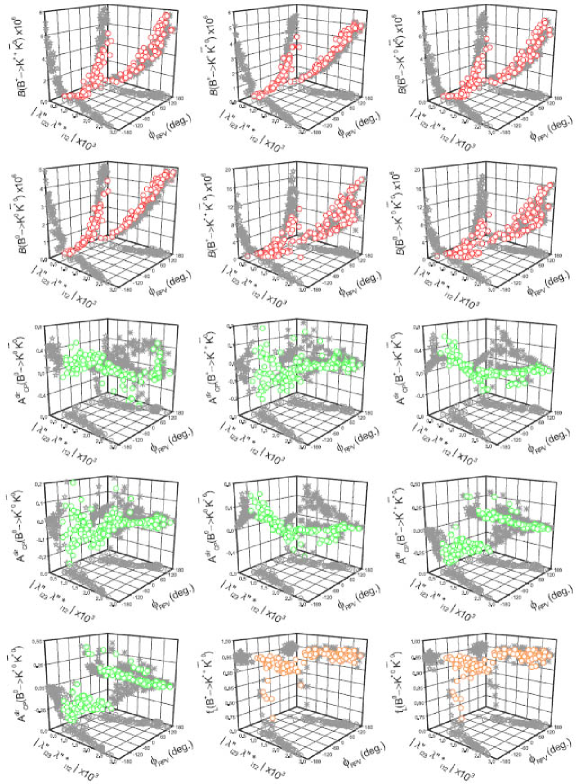
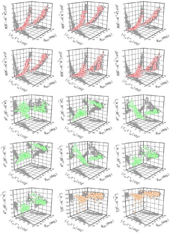
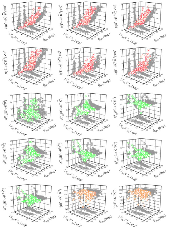
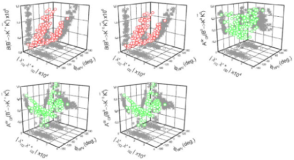
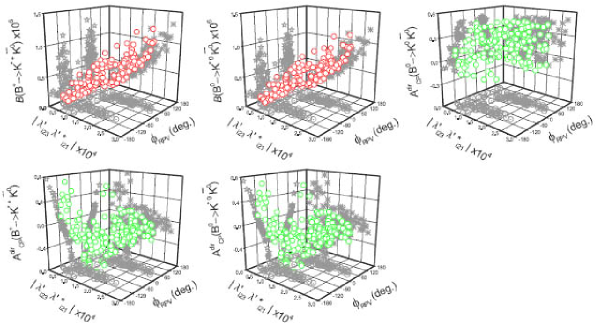
In Figs.6-10, we present correlations between the physical observable $\mathcal{B}$, $\mathcal{A}^{dir}_{CP}$, $f_{L}$ and the parameter spaces of different RPV couplings by the three-dimensional scatter plots. The more information are displayed in Figs.6-10, we can see the change trends of the physical observable quantities with the modulus and weak phase $\phi_{\not\!R_{p}\,}$ of RPV couplings. We take the first plot in Fig.6 as an example, this plot shows that $\mathcal{B}(B\rightarrow K^{*+}\bar{K}^{0})$ change trend with RPV coupling $\lambda^{\prime\prime}_{i23}\lambda^{\prime\prime*}_{i12}$. We also give projections on three vertical planes, the $|\lambda^{\prime\prime}_{i23}\lambda^{\prime\prime*}_{i12}|$-$\phi_{\not\!R_{p}\,}$ plane display the allowed regions of $\lambda^{\prime\prime}_{i23}\lambda^{\prime\prime*}_{i12}$ which satisfy experimental data in Eq.(34) (the same as the first plot in Fig.5). It’s shown that $\mathcal{B}(B\rightarrow K^{*+}\bar{K}^{0})$ is increasing with $|\lambda^{\prime\prime}_{i23}\lambda^{\prime\prime*}_{i12}|$ on the $\mathcal{B}(B\rightarrow K^{*+}\bar{K}^{0})$ -$|\lambda^{\prime\prime}_{i23}\lambda^{\prime\prime*}_{i12}|$ plane. From the $\mathcal{B}(B\rightarrow K^{*+}\bar{K}^{0})$-$\phi_{\not\!R_{p}\,}$ plane, we can see that $\mathcal{B}(B\rightarrow K^{*+}\bar{K}^{0})$ is increasing with $|\phi_{\not\!R_{p}\,}|$. Further refined measurements of $\mathcal{B}(B\rightarrow K^{*+}\bar{K}^{0})$ can further restrict the constrained space of $\lambda^{\prime\prime}_{i23}\lambda^{\prime\prime*}_{i12}$, whereas with more narrow space of $\lambda^{\prime\prime}_{i23}\lambda^{\prime\prime*}_{i12}$ more accurate $\mathcal{B}(B\rightarrow K^{*+}\bar{K}^{0})$ can be predicted.

The following salient features in Figs.6-10 are summarized as following.

• Fig.6 displays the effects of RPV coupling $\lambda^{\prime\prime}_{i23}\lambda^{\prime\prime*}_{i12}$ on $\mathcal{B}$, $\mathcal{A}^{dir}_{CP}$ and $f_{L}$ in $B\to K^{(*)}\bar{K}^{(*)}$. The constrained $|\lambda^{\prime\prime}_{i23}\lambda^{\prime\prime*}_{i12}|$-$\phi_{\not\!R_{p}\,}$ plane shows the allowed range of $\lambda^{\prime\prime}_{i23}\lambda^{\prime\prime*}_{i12}$ as in the first plot of Fig.5. The six $\mathcal{B}(B\to K^{*+}\bar{K}^{0},K^{+}\bar{K}^{*0},K^{*0}\bar{K}^{0},K^{0}\bar{K}^{*0},K^{*+}\bar{K}^{*0},K^{*0}\bar{K}^{*0})$ have the similar change trends with $|\lambda^{\prime\prime}_{i23}\lambda^{\prime\prime*}_{i12}|$ and $|\phi_{\not\!R_{p}\,}|$, and they are increasing with $|\lambda^{\prime\prime}_{i23}\lambda^{\prime\prime*}_{i12}|$ and $|\phi_{\not\!R_{p}\,}|$. $|\mathcal{A}^{dir}_{CP}(B\to K^{0}\bar{K}^{0})|$ are increasing with $|\phi_{\not\!R_{p}\,}|$, but $|\lambda^{\prime\prime}_{i23}\lambda^{\prime\prime*}_{i12}|$ has small effect on $\mathcal{A}^{dir}_{CP}(B\to K^{0}\bar{K}^{0})$. The two $|\mathcal{A}^{dir}_{CP}(B\to K^{+}\bar{K}^{*0},K^{0}\bar{K}^{*0})|$ tend to zero with increasing $|\lambda^{\prime\prime}_{i23}\lambda^{\prime\prime*}_{i12}|$ and $|\phi_{\not\!R_{p}\,}|$. The other four $|\mathcal{A}^{dir}_{CP}(B\to K^{*+}\bar{K}^{0},K^{*0}\bar{K}^{0},K^{*+}\bar{K}^{*0},K^{*0}\bar{K}^{*0})|$ tend to zero with increasing $|\phi_{\not\!R_{p}\,}|$, and they could have smaller ranges with $|\lambda^{\prime\prime}_{i23}\lambda^{\prime\prime*}_{i12}|$. The RPV effects on the $f_{L}(B\rightarrow K^{*+}\bar{K}^{*0},K^{*0}\bar{K}^{*0})$ are very small, and $f_{L}(B\rightarrow K^{*+}\bar{K}^{*0},K^{*0}\bar{K}^{*0})$ are found to lie between 0.72 and 0.97.

• The effects of $\lambda^{\prime}_{i13}\lambda^{\prime*}_{i22}$ on $\mathcal{B}$, $\mathcal{A}^{dir}_{CP}$ and $f_{L}$ are exhibited in Fig.7. The constrained $|\lambda^{\prime}_{i13}\lambda^{\prime*}_{i22}|$-$\phi_{\not\!R_{p}\,}$ plane is the same as the second plot in Fig.5. The effects of $\lambda^{\prime}_{i13}\lambda^{\prime*}_{i22}$ on $\mathcal{B}$, $\mathcal{A}^{dir}_{CP}$ and $f_{L}$ are similar to $\lambda^{\prime\prime}_{i23}\lambda^{\prime\prime*}_{i12}$ shown in Fig.6.

• In Fig.8, we plot $\mathcal{B}$, $\mathcal{A}^{dir}_{CP}$ and $f_{L}$ as functions of $\lambda^{\prime}_{i22}\lambda^{\prime*}_{i31}$. The constrained $|\lambda^{\prime}_{i22}\lambda^{\prime*}_{i31}|$-$\phi_{\not\!R_{p}\,}$ plane is the same as the third plot of Fig.5. The six branching ratios are increasing with $|\lambda^{\prime}_{i22}\lambda^{\prime*}_{i31}|$ and decreasing with $|\phi_{\not\!R_{p}\,}|$. $|\mathcal{A}^{dir}_{CP}(B\to K^{0}\bar{K}^{0})|$ is unaffected by $|\lambda^{\prime}_{i22}\lambda^{\prime*}_{i31}|$, but the other six direct CP asymmetries could have smaller ranges with $|\lambda^{\prime}_{i22}\lambda^{\prime*}_{i31}|$. $|\mathcal{A}^{dir}_{CP}(K^{*+}\bar{K}^{0},K^{*0}\bar{K}^{0})|$ tends to zero with decreasing $|\phi_{\not\!R_{p}\,}|$, however, $\phi_{\not\!R_{p}\,}$ has small effect on $\mathcal{A}^{dir}_{CP}(B\to K^{0}\bar{K}^{0},K^{+}\bar{K}^{*0},K^{0}\bar{K}^{*0},K^{*+}\bar{K}^{*0},K^{*0}\bar{K}^{*0})$. The $\lambda^{\prime}_{i22}\lambda^{\prime*}_{i31}$ effects on the $f_{L}(B\rightarrow K^{*+}\bar{K}^{*0},K^{*0}\bar{K}^{*0})$ are small.

• RPV coupling $\lambda^{\prime}_{i12}\lambda^{\prime*}_{i32}$ contributes to the decays $B\to K^{+}\bar{K}^{0},K^{0}\bar{K}^{0},K^{*+}\bar{K}^{0},K^{*0}\bar{K}^{0}$, and the effects are shown in Fig.9. The constrained $|\lambda^{\prime}_{i12}\lambda^{\prime*}_{i32}|$-$\phi_{\not\!R_{p}\,}$ plane is the same as the fourth plot in Fig.5. We can see that $\mathcal{B}(B\to K^{*+}\bar{K}^{0},K^{*0}\bar{K}^{0})$ are rising with $|\lambda^{\prime}_{i12}\lambda^{\prime*}_{i32}|$, and unaffected by $\phi_{\not\!R_{p}\,}$. $\mathcal{A}^{dir}_{CP}(B\to K^{0}\bar{K}^{0})$ is steady against $|\lambda^{\prime}_{i12}\lambda^{\prime*}_{i32}|$, and $|\mathcal{A}^{dir}_{CP}(B\to K^{*+}\bar{K}^{0},K^{*0}\bar{K}^{0})|$ could have smaller ranges with $|\lambda^{\prime}_{i12}\lambda^{\prime*}_{i32}|$. $\mathcal{A}^{dir}_{CP}(B\to K^{0}\bar{K}^{0},K^{*+}\bar{K}^{0},$ $K^{*0}\bar{K}^{0})$ are becoming large with increasing of $|\phi_{\not\!R_{p}\,}|$.

• $\lambda^{\prime}_{i23}\lambda^{\prime*}_{i21}$ also only contributes to the decays $B\to K^{+}\bar{K}^{0},K^{0}\bar{K}^{0},K^{*+}\bar{K}^{0},K^{*0}\bar{K}^{0}$, and its effects are shown in Fig.10. The constrained $|\lambda^{\prime}_{i23}\lambda^{\prime*}_{i21}|$-$\phi_{\not\!R_{p}\,}$ plane is the same as the last plot in Fig.5. $\mathcal{B}(B\to K^{*+}\bar{K}^{0},K^{*0}\bar{K}^{0})$ are increasing with $|\lambda^{\prime}_{i23}\lambda^{\prime*}_{i21}|$, and unaffected by $\phi_{\not\!R_{p}\,}$. $\mathcal{A}^{dir}_{CP}(B\to K^{0}\bar{K}^{0})$ is steady against $|\lambda^{\prime}_{i23}\lambda^{\prime*}_{i21}|$, and $|\mathcal{A}^{dir}_{CP}(B\to K^{*+}\bar{K}^{0},K^{*0}\bar{K}^{0})|$ could be varied in small ranges with $|\lambda^{\prime}_{i23}\lambda^{\prime*}_{i21}|$. $\mathcal{A}^{dir}_{CP}(B\to K^{0}\bar{K}^{0})$ is decreasing with $|\phi_{\not\!R_{p}\,}|$, but $\mathcal{A}^{dir}_{CP}(B\to K^{*+}\bar{K}^{0},K^{*0}\bar{K}^{0})$ are increasing with $|\phi_{\not\!R_{p}\,}|$.

The predictions of $\mathcal{B}$ and $\mathcal{A}^{dir}_{CP}$ are quite uncertain in the RPV SUSY, since we just have few experimental measurements and many theoretical uncertainties. One must wait for the error bars to come down and more channels measured. With the operation of $B$ factory experiments, large amounts of experimental data on hadronic $B$ meson decays are being collected, and measurements of previously known observable will become more precise. From the comparison of our predictions in Figs.6-10 with the near future experiments, one will obtain more stringent bounds on the product combinations of RPV couplings. On the other hand, the RPV SUSY predictions of other decays will become more precise by the more stringent bounds on the RPV couplings.

5 Conclusions

In conclusions, the pure penguin $B\to K^{(*)}\bar{K}^{(*)}$ decays are very important for understanding the dynamics of nonleptonic two-body $B$ decays and testing the SM. We have studied the $B\to K^{(*)}\bar{K}^{(*)}$ decays with the QCDF approach in the RPV SUSY model. We have obtained fairly constrained parameter spaces of the RPV couplings from the present experimental data of $B\to K^{(*)}\bar{K}^{(*)}$ decays, and some of these constraints are stronger than the existing ones. Furthermore, using the constrained parameter spaces, we have shown the RPV SUSY expectations for the other quantities in $B\to K^{(*)}\bar{K}^{(*)}$ decays which have not been measured yet. We have found that the RPV effects could significantly alter $\mathcal{B}$ and $\mathcal{A}^{dir}_{CP}$ from their SM values, but $f_{L}(B\rightarrow K^{*+}\bar{K}^{*0},K^{*0}\bar{K}^{*0})$ are not significantly affected by the RPV effects and the decays $B\rightarrow K^{*+}\bar{K}^{*0},K^{*0}\bar{K}^{*0}$ are still dominated by the longitudinal polarization. We also have presented correlations between the physical observable $\mathcal{B}$, $\mathcal{A}^{dir}_{CP}$, $f_{L}$ and the constrained parameter spaces of RPV couplings in Figs.6-10, which could be tested in the near future.

Appendix A . Correction functions for $B\to M_{1}M_{2}$ decay at $\alpha_{s}$ order

In this appendix, we present the explicit form for the correction functions appearing in the parameters $a^{p}_{i}$ and $b^{p}_{i}$. It’s noted that in $B\to PV$ decays, $\Phi_{M}(u)\rightarrow\Phi^{V}_{\parallel}(u)$ if M a vector meson.

A.1 The correction functions in $B\to PP,PV$ decays

$\bullet$ One-loop vertex correction function is

$$V_{M_{2}}=12\ln\frac{m_{b}}{\mu}-18+3\int_{0}^{1}{\rm d}u\left(\frac{1-2u}{1-u}\ln u-i\pi\right)\Phi_{M_{2}}(u).$$ (37)

$\bullet$ The hard spectator interactions are given by

$$H_{M_{1}M_{2}}=\frac{4\pi^{2}}{N_{C}}\frac{f_{B}f_{M_{1}}}{m_{B}^{2}F_{0}^{B\to M_{1}}(m^{2}_{M_{2}})}\int^{1}_{0}\frac{{\rm d}\xi}{\xi}\Phi^{B}_{1}(\xi)\int^{1}_{0}\frac{{\rm d}u}{\bar{u}}\Phi_{M_{2}}(u)\int^{1}_{0}\frac{{\rm d}v}{\bar{v}}\left[\Phi_{M_{1}}(v)+\frac{2\mu_{M_{1}}}{M_{B}}\Phi^{M_{1}}_{p}(v)\right],$$ (38)

if $M_{2}$ is a pseudoscalar meson, and

$$H_{M_{1}M_{2}}=\frac{4\pi^{2}}{N_{C}}\frac{f_{B}f_{M_{1}}}{m_{B}^{2}A_{0}^{B\to M_{1}}(m^{2}_{M_{2}})}\int^{1}_{0}\frac{{\rm d}\xi}{\xi}\Phi^{B}_{1}(\xi)\int^{1}_{0}\frac{{\rm d}u}{\bar{u}}\Phi_{M_{2}}(u)\int^{1}_{0}\frac{{\rm d}v}{\bar{v}}\Phi_{M_{1}}(v),$$ (39)

if $M_{2}$ is a vector meson.

Considering the off-shellness of the gluon in hard scattering kernel, it is natural to associate a scale $\mu_{h}\sim\sqrt{\Lambda_{QCD}m_{b}}$ , rather than $\mu\sim m_{b}$. For the logarithmically divergent integral, we will parameterize it as in [17]: $X_{H}=\int^{1}_{0}{\rm d}u/u=-ln(\Lambda_{QCD}/m_{b})+\varrho_{H}e^{i\phi_{H}}$ $m_{b}/\Lambda_{QCD}$ with $(\varrho_{H},\phi_{H})$ related to the contributions from hard spectator scattering. In the numerical analysis, we take $\Lambda_{QCD}=0.5GeV$, $(\varrho_{h},\phi_{H})=(0,0)$ as our default values. The same as in $B\to VV$ decay.

$\bullet$ The penguin contributions at the twist-2 are described by the functions

$$P^{p}_{M_{2},2} = C_{1}G_{M_{2}}(s_{p})+C_{3}\Big{[}G_{M_{2}}(0)+G_{M_{2}}(1)\Big{]}+(C_{4}+C_{6})\bigg{[}(n_{f}-2)G_{M_{2}}(0)$$

$$+~{}G_{M_{2}}(s_{c})+G_{M_{2}}(1)-\frac{2n_{f}}{3}\bigg{]}-C^{eff}_{8g}\int_{0}^{1}{\rm d}u~{}\frac{2\Phi_{M_{2}}(u)}{1-u},$$

$$P^{p,EW}_{M_{2},2} = (C_{1}+N_{C}C_{2})G_{M_{2}}(s_{p})-~{}C^{eff}_{7\gamma}\int_{0}^{1}{\rm d}u~{}\frac{3\Phi_{M_{2}}(u)}{1-u},$$ (40)

where $n_{f}=5$ is the number of quark flavors, and $s_{u}=0,s_{c}=(m_{c}/m_{b})^{2}$ are mass ratios involved in the evaluation of the penguin diagrams. The function $G_{M_{2}}(s)$ is defined as

$$G_{M_{2}}(s)=\frac{2}{3}+\frac{4}{3}\ln\frac{m_{b}}{\mu}+4\int_{0}^{1}{\rm d}u\int_{0}^{1}{\rm d}x~{}x\bar{x}\ln{(s-x\bar{x}\bar{u}-i\epsilon)}\Phi_{M_{2}}(u).$$ (41)

$\bullet$ The twist-3 terms from the penguin diagrams are given by

$$P^{p}_{M_{2},3} = C_{1}\widehat{G}_{M_{2}}(s_{p})+C_{3}\left[\widehat{G}_{M_{2}}(0)+\widehat{G}_{M_{2}}(1)\right]+~{}(C_{4}+C_{6})\bigg{[}(n_{f}-2)\widehat{G}_{M_{2}}(0)$$

$$+~{}\widehat{G}_{M_{2}}(s_{c})+\widehat{G}_{M_{2}}(1)-\frac{2n_{f}}{3}\bigg{]}-~{}2C^{eff}_{8g},$$

$$P^{p,EW}_{M_{2},3} = (C_{1}+N_{C}C_{2})\widehat{G}_{M_{2}}(s_{p})-~{}3C^{eff}_{7\gamma},$$ (42)

with

$$\widehat{G}_{M_{2}}(s)=\frac{2}{3}+\frac{4}{3}\ln\frac{m_{b}}{\mu}+4\int_{0}^{1}{\rm d}u\int_{0}^{1}{\rm d}x~{}x\bar{x}\ln{(s-x\bar{x}\bar{u}-i\epsilon)}\Phi^{M_{2}}_{p}(u),$$ (43)

if $M_{2}$ is a pseudoscalar meson, and we omit the twist-3 terms from the penguin diagrams when $M_{2}$ is a vector meson.

$\bullet$ The weak annihilation contributions are given by

$$A^{i}_{1}(M_{1},M_{2})\approx A^{i}_{2}(M_{1},M_{2})\approx\pi\alpha_{s}\left[18\left(X_{A}-4+\frac{\pi^{2}}{3}\right)+2r^{M_{1}}_{\chi}r^{M_{2}}_{\chi}X^{2}_{A}\right],$$

$$A^{i}_{3}(M_{1},M_{2})\approx 6\pi\alpha_{s}(r^{M_{1}}_{\chi}-r^{M_{2}}_{\chi})\left(X^{2}_{A}-2X_{A}+\frac{\pi^{2}}{3}\right),$$

$$A^{f}_{3}(M_{1},M_{2})\approx 6\pi\alpha_{s}(r^{M_{1}}_{\chi}+r^{M_{2}}_{\chi})\left(2X^{2}_{A}-X_{A}\right),$$

$$A^{f}_{1}(M_{1},M_{2})=0,~{}~{}~{}~{}~{}A^{f}_{2}(M_{1},M_{2})=0.$$ (44)

when both final state mesons are pseudoscalar, whereas

$$A^{i}_{1}(M_{1},M_{2})\approx-A^{i}_{2}(M_{1},M_{2})\approx 18\pi\alpha_{s}\left(X_{A}-4+\frac{\pi^{2}}{3}\right),$$

$$A^{i}_{3}(M_{1},M_{2})\approx 6\pi\alpha_{s}r^{M_{1}}_{\chi}\left(X^{2}_{A}-2X_{A}+\frac{\pi^{2}}{3}\right),$$

$$A^{f}_{3}(M_{1},M_{2})\approx-6\pi\alpha_{s}r^{M_{1}}_{\chi}\left(2X^{2}_{A}-X_{A}\right),$$

$$A^{f}_{1}(M_{1},M_{2})=0,~{}~{}~{}~{}~{}A^{f}_{2}(M_{1},M_{2})=0.$$ (45)

when $M_{1}$ is a vector meson and $M_{2}$ is a pseudoscalar. For the opposite case of a pseudoscalar $M_{1}$ and a vector $M_{2}$, one exchanges $r^{M_{1}}_{\chi}\leftrightarrow r^{M_{2}}_{\chi}$ in the previous equations and changes the sign of $A^{f}_{3}$.

Here the superscripts $i$ and $f$ refer to gluon emission from the initial and final state quarks, respectively. The subscript $k$ of $A^{i,f}_{k}$ refers to one of the three possible Dirac structures $\Gamma_{1}\otimes\Gamma_{2}$, namely $k=1$ for $(V-A)\otimes(V-A)$, $k=2$ for $(V-A)\otimes(V+A)$, and $k=3$ for $(-2)(S-P)\otimes(S+P)$. $X_{A}=\int^{1}_{0}{\rm d}u/u$ is a logarithmically divergent integral, and will be phenomenologically parameterized in the calculation as $X_{H}$. As for the hard spectator terms, we will evaluate the various quantities in Eqs. (44) and (45) at the scale $\mu_{h}=\sqrt{\Lambda_{QCD}m_{b}}$.

A.2 $B\to VV$ decays

In the rest frame of $B$ system, since the $B$ meson has spin zero, two vectors have the same helicity therefore three polarization states are possible, one longitudinal (L) and two transverse, corresponding to helicities $\lambda=0$ and $\lambda=\pm$ ( here $\lambda_{1}=\lambda_{2}=\lambda$). We assume the $M_{1}$($M_{2}$) meson flying in the minus(plus) z-direction carrying the momentum $p_{1}$($p_{2}$), Using the sign convention $\epsilon^{0123}=-1$, we have

$$A_{M_{1}M_{2}}=\left\{\begin{array}[]{ll}\frac{if_{M_{2}}}{2m_{M_{1}}}\left[(m^{2}_{B}-m_{M_{1}}^{2}-m_{M_{2}}^{2})(m_{B}+m_{M_{1}})A_{1}^{B\to M_{1}}(m_{M_{2}}^{2})-\frac{4m_{B}^{2}p_{c}^{2}}{m_{B}+m_{M_{1}}}A_{2}^{B\to M_{1}}(m_{M_{2}}^{2})\right]\equiv h_{0},\\ if_{V_{2}}m_{M_{2}}[(m_{B}+m_{M_{1}})A_{1}^{B\to M_{1}}(m_{M_{2}}^{2})\mp\frac{2m_{B}p_{c}}{m_{B}+m_{M_{1}}}V^{B\to M_{1}}(m_{M_{2}}^{2})]\equiv h_{\pm},\end{array}\right.$$ (48)

where $h_{0}$ for $\lambda=0$ and $h_{\pm}$ for $\lambda=\pm$.

$\bullet$ $V_{M_{2}}^{\lambda}(\pm 1)$ contain the contributions from the vertex corrections, and given by

$$V_{M_{2}}^{0}(a)=12\ln\frac{m_{b}}{\mu}-18+\int_{0}^{1}{\rm d}u\Phi_{\parallel}^{M_{2}}(u)\left(3\frac{1-2u}{1-u}\ln u-3i\pi\right),$$ (49)

$$V_{M_{2}}^{\pm}(a)=12\ln\frac{m_{b}}{\mu}-18+\int_{0}^{1}{\rm d}u\left(\mbox{g}_{\perp}^{(v){M_{2}}}(u)\pm\frac{a\mbox{g}_{\perp}^{\prime(a){M_{2}}}(u)}{4}\right)\left(3\frac{1-2u}{1-u}\ln u-3i\pi\right).$$

$\bullet$ The hard spectator scattering contributions, explicit calculations for $H_{M_{1}M_{2}}^{\lambda}(a)$ yield

$$H_{M_{1}M_{2}}^{0}(a) = \frac{4\pi^{2}}{N_{C}}\frac{if_{B}f_{V_{1}}f_{V_{2}}}{h_{0}}\int_{0}^{1}{\rm d}\xi\frac{\Phi_{1}^{B}(\xi)}{\xi}\int_{0}^{1}{\rm d}v\frac{\Phi_{\parallel}^{M_{1}}(v)}{\bar{v}}\int_{0}^{1}{\rm d}u\frac{\Phi_{\parallel}^{M_{2}}(u)}{u},$$

$$H_{M_{1}M_{2}}^{\pm}(a) = -\frac{4\pi^{2}}{N_{C}}\frac{2if_{B}f^{\perp}_{M_{1}}f_{M_{2}}m_{M_{2}}}{m_{B}h_{\pm}}(1\mp 1)\int_{0}^{1}{\rm d}\xi\frac{\Phi_{1}^{B}(\xi)}{\xi}\int_{0}^{1}{\rm d}v\frac{\Phi_{\perp}^{M_{1}}(v)}{\bar{v}^{2}}$$ (50)

$$\times\int_{0}^{1}{\rm d}u\left(\mbox{g}_{\perp}^{(v){M_{2}}}(u)-\frac{a\mbox{g}_{\perp}^{\prime(a){M_{2}}}(u)}{4}\right)+\frac{4\pi^{2}}{N_{C}}\frac{2if_{B}f_{M_{1}}f_{M_{2}}m_{M_{1}}m_{M_{2}}}{m_{B}^{2}h_{\pm}}\int_{0}^{1}{\rm d}\xi\frac{\Phi_{1}^{B}(\xi)}{\xi}$$

$$\times\int_{0}^{1}{\rm d}v{\rm d}u\left(\mbox{g}_{\perp}^{(v){M_{1}}}(v)\pm\frac{\mbox{g}_{\perp}^{\prime(a){M_{1}}}(v)}{4}\right)\left(\mbox{g}_{\perp}^{(v){M_{2}}}(u)\pm\frac{a\mbox{g}_{\perp}^{\prime(a){M_{2}}}(u)}{4}\right)\frac{u+\bar{v}}{u{\bar{v}}^{2}},$$

with $\bar{v}=1-v$, when the asymptotical form for the vector meson LCDAs adopted, there will be infrared divergences in $H_{M_{1}M_{2}}^{\pm}$. As in [16, 28], we introduce a cutoff of order $\Lambda_{QCD}/m_{b}$ and take $\Lambda_{QCD}=0.5$ GeV as our default value.

$\bullet$ The contributions of the QCD penguin-type diagrams can be described by the functions

$$P^{\lambda,p}_{M_{2},2} = C_{1}G^{\lambda}_{M_{2}}(s_{p})+C_{3}\left[G^{\lambda}_{M_{2}}(s_{q})+G^{\lambda}_{M_{2}}(s_{b})\right]+(C_{4}+C_{6})\sum_{q^{\prime}=u}^{b}\Big{[}G^{\lambda}_{M_{2}}(s_{q^{\prime}})-\frac{2}{3}\Big{]}$$

$$+\frac{3}{2}C_{9}\Big{[}e_{q}G^{\lambda}_{M_{2}}(s_{q})+e_{b}G^{\lambda}_{M_{2}}(s_{b})\Big{]}+\frac{3}{2}(C_{8}+C_{10})\sum_{q^{\prime}=u}^{b}e_{q^{\prime}}\Big{[}G^{\lambda}_{M_{2}}(s_{q^{\prime}})-\frac{2}{3}\Big{]}+C^{eff}_{8g}G_{g}^{\lambda},$$

$$P^{\lambda,p,EW}_{M_{2},2} = (C_{1}+N_{C}C_{2})\left[\frac{2}{3}+\frac{4}{3}\ln\frac{m_{b}}{\mu}-G^{\lambda}_{M_{2}}(s_{p})\right]+~{}\frac{3}{2}C^{eff}_{7\gamma}G^{\lambda}_{g},$$ (51)

$$G^{0}_{M_{2}}(s) = \frac{2}{3}+\frac{4}{3}\ln\frac{m_{b}}{\mu}+4\int_{0}^{1}{\rm d}u~{}\Phi_{\parallel}^{M_{2}}(u)\mbox{g}(u,s),$$

$$G^{\pm}_{M_{2}}(s) = \frac{2}{3}+\frac{2}{3}\ln\frac{m_{b}}{\mu}+2\int_{0}^{1}{\rm d}u~{}(\mbox{g}_{\perp}^{(v){M_{2}}}(u)\pm\frac{\mbox{g}_{\perp}^{\prime(a){M_{2}}}(u)}{4})\mbox{g}(u,s),$$ (52)

with the function g$(u,s)$ defined as

$$\mbox{g}(u,s) = \int_{0}^{1}{\rm d}x~{}x\bar{x}\ln{(s-x\bar{x}\bar{u}-i\epsilon)}.$$ (53)

We omit the twist-3 terms from the penguin diagrams for $B\to VV$ decays.

$\bullet$ We have also taken into account the contributions of the dipole operator $O_{8g}$, which are described by the functions

$$G_{g}^{0}=-\int_{0}^{1}{\rm d}u~{}\frac{2\Phi_{\parallel}^{M_{2}}(u)}{1-u},$$

$$G_{g}^{\pm}=\int_{0}^{1}~{}\frac{{\rm d}u}{\bar{u}}\left[-\bar{u}\mbox{g}_{\perp}^{(v){M_{2}}}(u)\mp\frac{\bar{u}\mbox{g}_{\perp}^{\prime(a){M_{2}}}(u)}{4}+\int_{0}^{u}{\rm d}v\left(\Phi_{\parallel}^{M_{2}}(v)-\mbox{g}_{\perp}^{(v)M_{2}}(v)\right)+\frac{\mbox{g}_{\perp}^{(a){M_{2}}}(u)}{4}\right],$$ (54)

here we consider the higher-twist effects $k^{\mu}=uEn_{-}^{\mu}+k_{\perp}^{\mu}+\frac{\vec{k}_{\perp}^{2}}{4uE}n_{+}^{\mu}$ in the projector of the vector meson. The $G_{g}^{\pm}=0$ in Eq.(54) [28, 30] if considering the Wandzura-Wilczek-type relations [29].

We have not onsidered the annihilation contributions in $B\to VV$ decays.

A.3 The contributions of new operators in RPV SUSY

Compared with the operators in the $\mathcal{H}^{SM}_{eff}$, there are new operators $(\bar{q}_{2}q_{3})_{V\pm A}(\bar{b}q_{1})_{V+A}$ in the $\mathcal{H}^{\not\!R_{p}\,}_{eff}$.

$\bullet$ For $B\to PP,PV$ decays, since

$$\langle P|~{}\bar{q}_{1}\gamma_{\mu}(1-\gamma_{5})q_{2}|~{}0\rangle=-\langle P|~{}\bar{q}_{1}\gamma_{\mu}(1+\gamma_{5})q_{2}|~{}0\rangle=-\langle P|~{}\bar{q}_{1}\gamma_{\mu}\gamma_{5}q_{2}|~{}0\rangle,$$

$$\langle P|~{}\bar{q}\gamma_{\mu}(1-\gamma_{5})b~{}|~{}B\rangle=\langle P|~{}\bar{q}\gamma_{\mu}(1+\gamma_{5})b~{}|~{}B\rangle=\langle P|~{}\bar{q}\gamma_{\mu}b~{}|~{}B\rangle,\hskip 28.45274pt$$

$$\langle V|~{}\bar{q}_{1}\gamma_{\mu}(1-\gamma_{5})q_{2}|~{}0\rangle=\langle V|~{}\bar{q}_{1}\gamma_{\mu}(1+\gamma_{5})q_{2}|~{}0\rangle=\langle V|~{}\bar{q}_{1}\gamma_{\mu}q_{2}|~{}0\rangle,$$

$$\langle V|~{}\bar{q}\gamma_{\mu}(1-\gamma_{5})b~{}|~{}B\rangle=-\langle V|~{}\bar{q}\gamma_{\mu}(1+\gamma_{5})b~{}|~{}B\rangle=-\langle V|~{}\bar{q}\gamma_{\mu}\gamma_{5}b~{}|~{}B\rangle,\hskip 28.45274pt$$ (55)

the RPV contribution to the decay amplitude will modify the SM amplitude by an overall relation.

$\bullet$ For $B\to VV$, we will use the prime on the quantities stands for the $(\bar{q}_{2}q_{3})_{V\pm A}(\bar{b}q_{1})_{V+A}$ current contribution. In the NF approach, the factorizable amplitude can be expressed as

$$A^{\prime}_{M_{1}M_{2}} = \langle M_{2}|(\bar{q}_{2}\gamma_{\mu}(1-a\gamma_{5})q_{3})|0\rangle\langle M_{1}|(\bar{b}\gamma^{\mu}(1+\gamma_{5})q_{1})|B\rangle.$$ (56)

Taking the $M_{1}$($M_{2}$) meson flying in the minus(plus) z-direction and using the sign convention $\epsilon^{0123}=-1$, we have

$$A^{\prime}_{M_{1}M_{2}}=\left\{\begin{array}[]{ll}\frac{-if_{M_{2}}}{2m_{M_{1}}}\left[(m^{2}_{B}-m_{M_{1}}^{2}-m_{M_{2}}^{2})(m_{B}+m_{M_{1}})A_{1}^{B\to M_{1}}(m_{M_{2}}^{2})-\frac{2m_{B}^{2}p_{c}^{2}}{m_{B}+m_{M_{1}}}A_{2}^{B\to M_{1}}(m_{M_{2}}^{2})\right]\equiv h^{\prime}_{0},\\ -if_{M_{2}}m_{M_{2}}\left[(m_{B}+m_{M_{1}})A_{1}^{B\to M_{1}}(m_{M_{2}}^{2})\pm\frac{2m_{B}p_{c}}{m_{B}+m_{M_{1}}}V^{B\to M_{1}}(m_{M_{2}}^{2})\right]\equiv h^{\prime}_{\pm}.\end{array}\right.$$ (59)

The vertex corrections $V^{{}^{\prime}\lambda}_{M_{2}}(a)$ and the hard spectator scattering corrections $H^{{}^{\prime}\lambda}_{M_{1}M_{2}}(a)$ as follows:

$$V_{M_{2}}^{{}^{\prime}0}(a) = -12\ln\frac{m_{b}}{\mu}+18-6(1+a)-\int_{0}^{1}{\rm d}u\Phi_{\parallel}^{M_{2}}(u)\left(3\frac{1-2u}{1-u}\ln u-3i\pi\right),$$

$$V_{M_{2}}^{{}^{\prime}\pm}(a) = -12\ln\frac{m_{b}}{\mu}+18-6(1+a)-\int_{0}^{1}{\rm d}u\left(g_{\perp}^{(v){M_{2}}}(u)\pm\frac{ag_{\perp}^{\prime(a){M_{2}}}(u)}{4}\right)\left(3\frac{1-2u}{1-u}\ln u-3i\pi\right),$$

$$H^{{}^{\prime}0}_{M_{1}M_{2}}(a) = \frac{4\pi^{2}}{N_{C}}\frac{if_{B}f_{M_{1}}f_{M_{2}}}{h^{{}^{\prime}}_{0}}\int_{0}^{1}{\rm d}\xi\frac{\Phi_{1}^{B}(\xi)}{\xi}\int_{0}^{1}{\rm d}v\frac{\Phi_{\parallel}^{M_{1}}(v)}{\bar{v}}\int_{0}^{1}{\rm d}u\frac{\Phi_{\parallel}^{M_{2}}(u)}{u},$$

$$H_{M_{1}M_{2}}^{{}^{\prime}\pm}(a) = -\frac{4\pi^{2}}{N_{C}}\frac{2if_{B}f^{\perp}_{M_{1}}f_{M_{2}}m_{M_{2}}}{m_{B}h^{{}^{\prime}}_{\pm}}(1\pm 1)\int_{0}^{1}{\rm d}\xi\frac{\Phi_{1}^{B}(\xi)}{\xi}\int_{0}^{1}{\rm d}v\frac{\Phi_{\perp}^{M_{1}}(v)}{\bar{v}^{2}}$$ (60)

$$\times\int_{0}^{1}{\rm d}u\left(g_{\perp}^{(v){M_{2}}}(u)+\frac{ag_{\perp}^{\prime(a){M_{2}}}(u)}{4}\right)+\frac{4\pi^{2}}{N_{C}}\frac{2if_{B}f_{M_{1}}f_{M_{2}}m_{M_{1}}m_{M_{2}}}{m_{B}^{2}h^{{}^{\prime}}_{\pm}}\int_{0}^{1}{\rm d}\xi\frac{\Phi_{1}^{B}(\xi)}{\xi}$$

$$\times\int_{0}^{1}{\rm d}v{\rm d}u\left(g_{\perp}^{(v){M_{1}}}(v)\mp\frac{g_{\perp}^{\prime(a){M_{1}}}(v)}{4}\right)\left(g_{\perp}^{(v){M_{2}}}(u)\pm\frac{ag_{\perp}^{\prime(a){M_{2}}}(u)}{4}\right)\frac{u+\bar{v}}{u{\bar{v}}^{2}}.$$

Appendix B . The amplitudes in the SM

$$\mathcal{A}^{SM}_{f}(B^{+}\rightarrow K^{+}\bar{K}^{0}) = \frac{G_{F}}{\sqrt{2}}\left\{-V^{*}_{tb}V_{td}\left[a_{4}-\frac{1}{2}a_{10}+r^{K^{0}}_{\chi}(a_{6}-\frac{1}{2}a_{8})\right]\right\}A_{K^{+}\bar{K}^{0}},$$ (61)

$$\mathcal{A}^{SM}_{a}(B^{+}\rightarrow K^{+}\bar{K}^{0}) = i\frac{G_{F}}{\sqrt{2}}f_{B}f^{2}_{K}\left\{V^{*}_{ub}V_{ud}b_{2}(K^{+},\bar{K}^{0})-V^{*}_{tb}V_{td}\left[b_{3}(K^{+},\bar{K}^{0})+b^{ew}_{3}(K^{+},\bar{K}^{0})\right]\right\},$$ (62)

$$\mathcal{A}^{SM}_{f}(B^{0}\rightarrow K^{0}\bar{K}^{0}) = \frac{G_{F}}{\sqrt{2}}\left\{-V^{*}_{tb}V_{td}\left[a_{4}-\frac{1}{2}a_{10}+r^{K^{0}}_{\chi}(a_{6}-\frac{1}{2}a_{8})\right]\right\}A_{K^{0}\bar{K}^{0}},$$ (63)

$$\mathcal{A}^{SM}_{a}(B^{0}\rightarrow K^{0}\bar{K}^{0}) = i\frac{G_{F}}{\sqrt{2}}f_{B}f^{2}_{K}\left\{-V^{*}_{tb}V_{td}\left[\frac{}{}b_{3}(\bar{K}^{0},K^{0})+b_{4}(\bar{K}^{0},K^{0})+b_{4}(K^{0},\bar{K}^{0})\right.\right.$$ (64)

$$\left.\left.-\frac{1}{2}b^{ew}_{3}(\bar{K}^{0},K^{0})-\frac{1}{2}b^{ew}_{4}(\bar{K}^{0},K^{0})-\frac{1}{2}b^{ew}_{4}(K^{0},\bar{K}^{0})\right]\right\},$$

$$\mathcal{A}^{SM}_{f}(B^{+}\rightarrow K^{*+}\bar{K}^{0}) = \frac{G_{F}}{\sqrt{2}}\left\{-V^{*}_{tb}V_{td}\left[a_{4}-\frac{1}{2}a_{10}-r^{K^{0}}_{\chi}(a_{6}-\frac{1}{2}a_{8})\right]\right\}A_{K^{*+}\bar{K}^{0}},$$ (65)

$$\mathcal{A}^{SM}_{a}(B^{+}\rightarrow K^{*+}\bar{K}^{0}) = \frac{G_{F}}{\sqrt{2}}f_{B}f_{K}f_{K^{*}}\left\{V^{*}_{ub}V_{ud}b_{2}(K^{*+},\bar{K}^{0})-V^{*}_{tb}V_{td}\left[b_{3}(K^{*+},\bar{K}^{0})+b^{ew}_{3}(K^{*+},\bar{K}^{0})\right]\right\},$$ (66)

$$\mathcal{A}^{SM}_{f}(B^{+}\rightarrow K^{+}\bar{K}^{*0}) = \frac{G_{F}}{\sqrt{2}}\left\{-V^{*}_{tb}V_{td}\left[a_{4}-\frac{1}{2}a_{10}\right]\right\}A_{K^{+}\bar{K}^{*0}},$$ (67)

$$\mathcal{A}^{SM}_{a}(B^{+}\rightarrow K^{+}\bar{K}^{*0}) = \frac{G_{F}}{\sqrt{2}}f_{B}f_{K}f_{K^{*}}\left\{V^{*}_{ub}V_{ud}b_{2}(K^{+},\bar{K}^{*0})-V^{*}_{tb}V_{td}\left[b_{3}(K^{+},\bar{K}^{*0})+b^{ew}_{3}(K^{+},\bar{K}^{*0})\right]\right\},$$ (68)

$$\mathcal{A}^{SM}_{f}(B^{0}\rightarrow K^{*0}\bar{K}^{0}) = \frac{G_{F}}{\sqrt{2}}\left\{-V^{*}_{tb}V_{td}\left[a_{4}-\frac{1}{2}a_{10}-r^{K^{0}}_{\chi}(a_{6}-\frac{1}{2}a_{8})\right]\right\}A_{K^{*0}\bar{K}^{0}},$$ (69)

$$\mathcal{A}^{SM}_{a}(B^{0}\rightarrow K^{*0}\bar{K}^{0}) = \frac{G_{F}}{\sqrt{2}}f_{B}f_{K}f_{K^{*}}\left\{-V^{*}_{tb}V_{td}\left[\frac{}{}b_{3}(K^{*0},\bar{K}^{0})+b_{4}(K^{*0},\bar{K}^{0})+b_{4}(\bar{K}^{0},K^{*0})\right.\right.$$ (70)

$$\left.\left.-\frac{1}{2}b^{ew}_{3}(K^{*0},\bar{K}^{0})-\frac{1}{2}b^{ew}_{4}(K^{*0},\bar{K}^{0})-\frac{1}{2}b^{ew}_{4}(\bar{K}^{0},K^{*0})\right]\right\},$$

$$\mathcal{A}^{SM}_{f}(B^{0}\rightarrow K^{0}\bar{K}^{*0}) = \frac{G_{F}}{\sqrt{2}}\left\{-V^{*}_{tb}V_{td}\left[a_{4}-\frac{1}{2}a_{10}\right]\right\}A_{K^{0}\bar{K}^{*0}},$$ (71)

$$\mathcal{A}^{SM}_{a}(B^{0}\rightarrow K^{0}\bar{K}^{*0}) = \frac{G_{F}}{\sqrt{2}}f_{B}f_{K}f_{K^{*}}\left\{-V^{*}_{tb}V_{td}\left[\frac{}{}b_{3}(K^{0},\bar{K}^{*0})+b_{4}(K^{0},\bar{K}^{*0})+b_{4}(\bar{K}^{*0},K^{0})\right.\right.$$ (72)

$$\left.\left.-\frac{1}{2}b^{ew}_{3}(K^{0},\bar{K}^{*0})-\frac{1}{2}b^{ew}_{4}(K^{0},\bar{K}^{*0})-\frac{1}{2}b^{ew}_{4}(\bar{K}^{*0},K^{0})\right]\right\},$$

$$\mathcal{A}^{SM}_{f}(B^{+}\rightarrow K^{*+}\bar{K}^{*0}) = \frac{G_{F}}{\sqrt{2}}\left\{-V^{*}_{tb}V_{td}\left[a_{4}-\frac{1}{2}a_{10}\right]\right\}A_{K^{*+}\bar{K}^{*0}},$$ (73)

$$\mathcal{A}^{SM}_{f}(B^{0}\rightarrow K^{*0}\bar{K}^{*0}) = \frac{G_{F}}{\sqrt{2}}\left\{-V^{*}_{tb}V_{td}\left[a_{4}-\frac{1}{2}a_{10}\right]\right\}A_{K^{*0}\bar{K}^{*0}},$$ (74)

Here we have not considered the annihilation contributions in $B\to VV$ decays.

Appendix C . The amplitudes for RPV

$$\mathcal{A}^{\not\!R\,_{p}}(B^{+}\rightarrow K^{+}\bar{K}^{0}) = \left\{\frac{\lambda^{\prime\prime}_{i23}\lambda^{\prime\prime*}_{i12}}{16m^{2}_{\tilde{u}_{i}}}\eta^{-4/\beta_{0}}F_{K^{+}\bar{K}^{0}}+\left(\frac{\lambda^{\prime}_{i13}\lambda^{\prime*}_{i22}}{8m^{2}_{\tilde{\nu}_{Li}}}-\frac{\lambda^{\prime}_{i22}\lambda^{\prime*}_{i31}}{8m^{2}_{\tilde{\nu}_{Li}}}\right)\eta^{-8/\beta_{0}}L_{K^{+}\bar{K}^{0}}\right.$$ (75)

$$\left.+\left(\frac{\lambda^{\prime}_{i12}\lambda^{\prime*}_{i32}}{8m^{2}_{\tilde{\nu}_{Li}}}-\frac{\lambda^{\prime}_{i23}\lambda^{\prime*}_{i21}}{8m^{2}_{\tilde{\nu}_{Li}}}\right)\eta^{-8/\beta_{0}}r^{K^{0}}_{\chi}\right\}A_{K^{+}\bar{K}^{0}},$$

$$\mathcal{A}^{\not\!R\,_{p}}(B^{0}\rightarrow K^{0}\bar{K}^{0}) = \left\{\frac{\lambda^{\prime\prime}_{i23}\lambda^{\prime\prime*}_{i12}}{16m^{2}_{\tilde{u}_{i}}}\eta^{-4/\beta_{0}}F_{K^{0}\bar{K}^{0}}+\left(\frac{\lambda^{\prime}_{i13}\lambda^{\prime*}_{i22}}{8m^{2}_{\tilde{\nu}_{Li}}}-\frac{\lambda^{\prime}_{i22}\lambda^{\prime*}_{i31}}{8m^{2}_{\tilde{\nu}_{Li}}}\right)\eta^{-8/\beta_{0}}L_{K^{0}\bar{K}^{0}}\right.$$ (76)

$$\left.+\left(\frac{\lambda^{\prime}_{i12}\lambda^{\prime*}_{i32}}{8m^{2}_{\tilde{\nu}_{Li}}}-\frac{\lambda^{\prime}_{i23}\lambda^{\prime*}_{i21}}{8m^{2}_{\tilde{\nu}_{Li}}}\right)\eta^{-8/\beta_{0}}r^{K^{0}}_{\chi}\right\}A_{K^{0}\bar{K}^{0}},$$

$$\mathcal{A}^{\not\!R\,_{p}}(B^{+}\rightarrow K^{*+}\bar{K}^{0}) = \left\{\frac{\lambda^{\prime\prime}_{i23}\lambda^{\prime\prime*}_{i12}}{16m^{2}_{\tilde{u}_{i}}}\eta^{-4/\beta_{0}}F_{K^{*+}\bar{K}^{0}}+\left(\frac{\lambda^{\prime}_{i13}\lambda^{\prime*}_{i22}}{8m^{2}_{\tilde{\nu}_{Li}}}+\frac{\lambda^{\prime}_{i22}\lambda^{\prime*}_{i31}}{8m^{2}_{\tilde{\nu}_{Li}}}\right)\eta^{-8/\beta_{0}}(-L_{K^{*+}\bar{K}^{0}})\right.$$ (77)

$$\left.-\left(\frac{\lambda^{\prime}_{i12}\lambda^{\prime*}_{i32}}{8m^{2}_{\tilde{\nu}_{Li}}}+\frac{\lambda^{\prime}_{i23}\lambda^{\prime*}_{i21}}{8m^{2}_{\tilde{\nu}_{Li}}}\right)\eta^{-8/\beta_{0}}r^{K^{0}}_{\chi}\right\}A_{K^{*+}\bar{K}^{0}},$$

$$\mathcal{A}^{\not\!R\,_{p}}(B^{+}\rightarrow K^{+}\bar{K}^{*0}) = \left\{\frac{\lambda^{\prime\prime}_{i23}\lambda^{\prime\prime*}_{i12}}{16m^{2}_{\tilde{u}_{i}}}\eta^{-4/\beta_{0}}F_{K^{+}\bar{K}^{*0}}+\left(\frac{\lambda^{\prime}_{i13}\lambda^{\prime*}_{i22}}{8m^{2}_{\tilde{\nu}_{Li}}}+\frac{\lambda^{\prime}_{i22}\lambda^{\prime*}_{i31}}{8m^{2}_{\tilde{\nu}_{Li}}}\right)\eta^{-8/\beta_{0}}L_{K^{+}\bar{K}^{*0}}\right\}A_{K^{+}\bar{K}^{*0}},$$ (78)

$$\mathcal{A}^{\not\!R\,_{p}}(B^{0}\rightarrow K^{*0}\bar{K}^{0}) = \left\{\frac{\lambda^{\prime\prime}_{i23}\lambda^{\prime\prime*}_{i12}}{16m^{2}_{\tilde{u}_{i}}}\eta^{-4/\beta_{0}}F_{K^{*0}\bar{K}^{0}}+\left(\frac{\lambda^{\prime}_{i13}\lambda^{\prime*}_{i22}}{8m^{2}_{\tilde{\nu}_{Li}}}+\frac{\lambda^{\prime}_{i22}\lambda^{\prime*}_{i31}}{8m^{2}_{\tilde{\nu}_{Li}}}\right)\eta^{-8/\beta_{0}}(-L_{K^{*0}\bar{K}^{0}})\right.$$ (79)

$$\left.-\left(\frac{\lambda^{\prime}_{i12}\lambda^{\prime*}_{i32}}{8m^{2}_{\tilde{\nu}_{Li}}}+\frac{\lambda^{\prime}_{i23}\lambda^{\prime*}_{i21}}{8m^{2}_{\tilde{\nu}_{Li}}}\right)\eta^{-8/\beta_{0}}r^{K^{0}}_{\chi}\right\}A_{K^{*0}\bar{K}^{0}},$$

$$\mathcal{A}^{\not\!R\,_{p}}(B^{0}\rightarrow K^{0}\bar{K}^{*0}) = \left\{\frac{\lambda^{\prime\prime}_{i23}\lambda^{\prime\prime*}_{i12}}{16m^{2}_{\tilde{u}_{i}}}\eta^{-4/\beta_{0}}F_{K^{0}\bar{K}^{*0}}+\left(\frac{\lambda^{\prime}_{i13}\lambda^{\prime*}_{i22}}{8m^{2}_{\tilde{\nu}_{Li}}}+\frac{\lambda^{\prime}_{i22}\lambda^{\prime*}_{i31}}{8m^{2}_{\tilde{\nu}_{Li}}}\right)\eta^{-8/\beta_{0}}L_{K^{0}\bar{K}^{*0}}\right\}A_{K^{0}\bar{K}^{*0}},$$ (80)

$$\mathcal{A}^{\not\!R\,_{p}}(B^{+}\rightarrow K^{*+}\bar{K}^{*0}) = \left\{\frac{\lambda^{\prime\prime}_{i23}\lambda^{\prime\prime*}_{i12}}{16m^{2}_{\tilde{u}_{i}}}\eta^{-4/\beta_{0}}F^{\prime}_{K^{*+}\bar{K}^{*0}}+\left(\frac{\lambda^{\prime}_{i13}\lambda^{\prime*}_{i22}}{8m^{2}_{\tilde{\nu}_{Li}}}\right)\eta^{-8/\beta_{0}}L^{\prime}_{K^{*+}\bar{K}^{*0}}\right\}A^{\prime}_{K^{*+}\bar{K}^{*0}}$$ (81)

$$+\frac{\lambda^{\prime}_{i22}\lambda^{\prime*}_{i31}}{8m^{2}_{\tilde{\nu}_{Li}}}L_{K^{*+}\bar{K}^{*0}}A_{K^{*+}\bar{K}^{*0}},$$

$$\mathcal{A}^{\not\!R\,_{p}}(B^{+}\rightarrow K^{*0}\bar{K}^{*0}) = \left\{\frac{\lambda^{\prime\prime}_{i23}\lambda^{\prime\prime*}_{i12}}{16m^{2}_{\tilde{u}_{i}}}\eta^{-4/\beta_{0}}F^{\prime}_{K^{*0}\bar{K}^{*0}}+\left(\frac{\lambda^{\prime}_{i13}\lambda^{\prime*}_{i22}}{8m^{2}_{\tilde{\nu}_{Li}}}\right)\eta^{-8/\beta_{0}}L^{\prime}_{K^{*0}\bar{K}^{*0}}\right\}A^{\prime}_{K^{*0}\bar{K}^{*0}}$$ (82)

$$+\frac{\lambda^{\prime}_{i22}\lambda^{\prime*}_{i31}}{8m^{2}_{\tilde{\nu}_{Li}}}L_{K^{*0}\bar{K}^{*0}}A_{K^{*0}\bar{K}^{*0}}.$$

In the $\mathcal{A}^{\not\!R\,_{p}}$, $F^{(^{\prime})}_{M_{1}M_{2}}$ and $L^{(^{\prime})}_{M_{1}M_{2}}$ are defined as

$$F_{M_{1}M_{2}} \equiv 1-\frac{1}{N_{C}}+\frac{\alpha_{s}}{4\pi}\frac{C_{F}}{N_{C}}\Big{[}V_{M_{2}}+H_{M_{1}M_{2}}\Big{]},$$ (83)

$$L_{M_{1}M_{2}} \equiv \frac{1}{N_{C}}\left\{1-\frac{\alpha_{s}}{4\pi}\frac{C_{F}}{N_{C}}\Big{[}12+V_{M_{2}}+H_{M_{1}M_{2}}\Big{]}\right\},$$ (84)

for $B\rightarrow PP,PV$ decays, and

$$F^{\prime}_{M_{1}M_{2}} \equiv 1-\frac{1}{N_{C}}-\frac{\alpha_{s}}{4\pi}\frac{C_{F}}{N_{C}}\left[V^{\prime\lambda}_{M_{2}}(-1)+H^{\prime\lambda}_{M_{1}M_{2}}(-1)\right],$$ (85)

$$L^{\prime}_{M_{1}M_{2}} \equiv \frac{1}{N_{C}}\left\{1+\frac{\alpha_{s}}{4\pi}\frac{C_{F}}{N_{C}}\left[-12+V^{\prime\lambda}_{M_{2}}(1)+H^{\prime\lambda}_{M_{1}M_{2}}(1)\right]\right\},$$ (86)

$$L_{M_{1}M_{2}} \equiv \frac{1}{N_{C}}\left\{1-\frac{\alpha_{s}}{4\pi}\frac{C_{F}}{N_{C}}\left[12+V^{\lambda}_{M_{2}}(-1)+H^{\lambda}_{M_{1}M_{2}}(-1)\right]\right\},$$ (87)

for $B\rightarrow VV$ decays.

Figure 6: The effects of RPV coupling $\lambda^{\prime\prime}_{i23}\lambda^{\prime\prime*}_{i12}$ in $B\to K^{(*)}\bar{K}^{(*)}$ decays.

Figure 7: The effects of RPV coupling $\lambda^{\prime}_{i13}\lambda^{\prime*}_{i22}$ in $B\to K^{(*)}\bar{K}^{(*)}$ decays.

Figure 8: The effects of RPV coupling $\lambda^{\prime}_{i22}\lambda^{\prime*}_{i31}$ in $B\to K^{(*)}\bar{K}^{(*)}$ decays.

Figure 9: The effects of RPV coupling $\lambda^{\prime}_{i12}\lambda^{\prime*}_{i32}$ in $B\to K^{(*)}\bar{K}^{(*)}$ decays.

Figure 10: The effects of RPV coupling $\lambda^{\prime}_{i23}\lambda^{\prime*}_{i21}$ in $B\to K^{(*)}\bar{K}^{(*)}$ decays.

References

- [1] A. J. Buras et al., Phys. Rev. Lett. 92, 101804(2004); Nucl. Phys. B697,133(2004).
- [2] B. Aubert et al. (BABAR Collaboration), Phys. Rev. Lett. 93, 231804(2004); K. F. Chen et al. (Belle Collaboration), Phys. Rev. Lett. 94, 221804(2005).
- [3] S. Weinberg, Phys. Rev. D26, 287(1982); N. Sakai and T. Yanagida, Nucl. Phys. B197, 533(1982); C. Aulakh and R. Mohapatra, Phys. Lett. B119, 136(1982).
- [4] See, for examaple, R. Barbier et al., hep-ph/9810232, Phys. Rept. 420, 1(2005), and references therein; M. Chemtob, Prog. Part. Nucl. Phys. 54, 71(2005).
- [5] B. C. Allanach et al., hep-ph/9906224, and references therein.
- [6] G. Bhattacharyya and A. Raychaudhuri, Phys. Rev. D57, R3837(1998); D. Guetta, Phys. Rev. D58, 116008(1998); G. Bhattacharyya and A. Datta, Phys. Rev. Lett. 83, 2300(1999); G. Bhattacharyya, A. Datta and A. Kundu, Phys. Lett. B514, 47(2001); D. Chakraverty and D. Choudhury, Phys. Rev. D63, 075009(2001); D. Chakraverty and D. Choudhury, Phys. Rev. D63, 112002(2001); J.P. Saha and A. Kundu, Phys. Rev. D66, 054021(2002); D. Choudhury, B. Dutta and A. Kundu, Phys. Lett. B456, 185(1999); G. Bhattacharyya, A. Datta and A. Kundu, J. Phys. G30, 1947(2004); B. Dutta, C.S. Kim and S. Oh, Phys. Rev. Lett. 90, 011801(2003); A. Datta, Phys. Rev. D66, 071702(2002); C. Dariescu, M.A. Dariescu, N.G. Deshpande and D.K. Ghosh, Phys. Rev. D69, 112003(2004); S. Bar-Shalom, G. Eilam and Y.D. Yang, Phys. Rev. D67, 014007(2003).
- [7] D. K. Ghosh, X. G. He, B. H. J. McKellar and J.Q. Shi, JHEP 0207, 067(2002).
- [8] Y. D. Yang, R. M. Wang and G. R. Lu, Phys. Rev. D72, 015009(2005); Phys. Rev. D73, 015003(2006).
- [9] Jin Zhu, Yue Long Shen and Cai Dian Lü, Phys. Rev. D72, 054015(2005); Cai Dian Lü, Yue Long Shen and Wei Wang, Phys. Rev. D73, 034005(2006); Jian Feng Cheng, Yuan Ning Gao, Chao Shang Huang and Xiao Hong Wu, hep-ph/0512268; C.W. Bauer, I.Z. Rothstein and I.W. Stewart, hep-ph/0510241; A. Datta and D. London, Phys. Lett. B533, 65(2002).
- [10] M. Beneke, G. Buchalla, M. Neubert and C. T. Sachrajda, Phys. Rev. Lett. 83, 1914(1999); Nucl. Phys. B591, 313(2000); Nucl. Phys. B606, 245(2001).
- [11] G. Buchalla, A. J. Buras and M. E. Lauteubacher, Rev. Mod. Phys. 68, 1125(1996).
- [12] M. Wirbel, B. Stech and M. Bauer, Zeit. Phys. C29, 637(1985); M. Bauer, B. Stech and M. Wirbel, Zeit. Phys. C34, 103(1987).
- [13] A. Ali et al., Phys. Rev. D58, 094009(1998); Phys. Rev. D59, 014005(1999).
- [14] Y. Y. Keum, H. n. Li and A. I. Sanda, Phys. Lett. B504, 6(2001); Phys. Rev. D63, 054008(2001); Y. Y. Keum and H. n. Li, Phys. Rev. D63, 074006(2001); C. D. L, K. Ukai and M.Z. Yang, Phys. Rev. D63, 074009(2001); Y. Y. Keum and A. I. Sanda, Phys. Rev. D67, 054009(2003).
- [15] P. Ball and R. Zwicky, Phys. Rev. D71, 014015(2005); Phys. Rev. D71, 014029(2005).
- [16] M. Beneke, G. Buchalla, M. Neubert and C. T. Sachrajda, Nucl. Phys. B606, 245(2001).
- [17] M. Beneke and M. Neubert, Nucl. Phys. B675, 333(2003).
- [18] S. Weinberg, Phys. Rev. D26, 287(1982).
- [19] R. Barbier et al., Phys. Rept. 420, 1(2005).
- [20] G. Bhattacharyya, A. Datta and A. Kundu, J. Phys. G30, 1947(2004).
- [21] S. Eidelman, et al. Phys. Lett. B592, 1(2004) and 2005 partial update for the 2006 edition available on the PDG WWW pages (URL: ).
- [22] V. M. Braun and I. E. Filyanov, Z. Phys. C48, 239(1990).
- [23] V. L. Chernyak and A. R. Zhitinissky, Phys. Rept. 112, 173(1984).
- [24] P. Ball and V.M. Braun, Nucl. Phys. B543, 201(1999).
- [25] V. M. Braun, D. Yu. Ivanov and G. P. Korchemsky, Phys. Rev. D69, 034014(2004).
- [26] B. Aubert et al. (BABAR Collaboration), Phys. Rev. Lett. 95, 221801(2005); B. Aubert et al. (BABAR Collaboration), hep-ex/0408080; K. Abe et al. (Belle Collaboration), Phys. Rev. Lett. 95, 231802(2005); A. Bornheim et al. (CLEO Collaboration), Phys. Rev., D68, 052002(2003); R. Godang et al. (CLEO Collaboration), Phys. Rev. Lett. 88, 021802(2002).
- [27] Heavy Flavor Averaging Group, hep-ex/0603003.
- [28] P. Kumar Das and Kwei-Chou Yang, Phys. Rev. D71, 094002(2005).
- [29] P. Ball et al., Nucl. Phys. B529, 323(1998).
- [30] A. Kagan, Phys. Lett. B601, 151(2004).