Fermion masses and proton decay in a minimal five-dimensional SO(10) model

Maria Laura Alciati     Ferruccio Feruglio     Yin Lin 

Dipartimento di Fisica ‘G. Galilei’, Università di Padova

INFN, Sezione di Padova, Via Marzolo 8, I-35131 Padua, Italy

Alvise Varagnolo 

Scuola Normale Superiore, Pisa

INFN, Sezione di Pisa, I-56126 Pisa, Italy

We propose a minimal SO(10) model in 5 space-time dimensions. The single extra spatial dimension is compactified on the orbifold $S^{1}/(Z_{2}\times Z_{2}^{\prime})$ reducing the gauge group to that of Pati-Salam $SU(4)_{C}\times SU(2)_{L}\times SU(2)_{R}$. The breaking down to the standard model group is obtained through an ordinary Higgs mechanism taking place at the Pati-Salam brane, giving rise to a proper gauge coupling unification. We achieve a correct description of fermion masses and mixing angles by describing first and second generations as bulk fields, and by embedding the third generation into four multiplets located at the Pati-Salam brane. The Yukawa sector is simple and compact and predicts a neutrino spectrum of normal hierarchy type. Concerning proton decay, dimension five operators are absent and the essentially unique localization of matter multiplets implies that the minimal couplings between the super-heavy gauge bosons and matter fields are vanishing. Non-minimal interactions are allowed but the resulting dimension six operators describing proton decay are too suppressed to produce observable effects, even in future, super-massive detectors.

1 Introduction

Despite the absence of any direct experimental check, the idea of grand unification is so deeply influencing our present view of particle physics that it has become a standard ingredient of most of the constructions extending the Standard Model (SM). It is however a matter of fact that all the advantages of grand unification, such as gauge coupling unification, particle classification, charge quantization, are quite difficult to incorporate into a complete and consistent picture. All simple realizations based on the standard tools of four-dimensional (4D) quantum field theory (QFT) face severe problems like the doublet-triplet (DT) splitting problem, a too fast proton decay, wrong fermion mass relations and unsatisfactory gauge coupling unification beyond the leading order. Non-minimal 4D versions of GUTs exist, which offer solutions to some or all the above mentioned problems, but very often these constructions make use of elaborate epicycles that spoil the beauty of the original GUT ideas, in order to be viable [1]. Quite often the necessity of these complicated constructions arises from the highly non trivial sector needed to successfully break the GUT symmetry, to naturally produce the DT splitting and to correctly break the flavour symmetries of the theory.

These difficulties have eventually led to the idea that in nature, perhaps, grand unification is not realized as a conventional 4D QFT. Examples of non conventional realizations of grand unification can be found in the context of string theory where, in some circumstances, the GUT symmetry becomes manifest only in the presence of the complete string spectrum. Working at the level of QFTs, successful versions of GUTs have been formulated in a higher dimensional space-time [2, 3, 4, 5, 6, 7]. Indeed, going to higher dimensions, several GUT problems find simple and elegant solutions [2]. For instance in SU(5), by allowing a single compact extra dimension, the GUT symmetry can be efficiently broken down to the SM gauge group by the compactification mechanism, without including any Higgs multiplet. Moreover this reduction of the gauge symmetry automatically entails a DT splitting, as soon as the 5 and $\bar{5}$ Higgs representations are introduced as 5D fields. Also gauge coupling unification, analyzed at the next-to-leading order can benefit [6, 7] from this framework . The size of the required extra dimension(s) is tiny since its inverse sets the grand unified scale. Thus the extra space does not have a direct impact on the gauge hierarchy problem. However it can highly affect our description of flavour physics because Yukawa couplings are strictly related to the localization properties of matter in the extra compact space [8].

Higher-dimensional GUTs make specific predictions about proton decay, which represents the ultimate experimental test of grand unification. For instance, in 5D supersymmetric (SUSY) SU(5), dimension 5 operators arising through coloured higgsino exchange are forbidden by an abelian continuous symmetry, thus avoiding the dominant and problematic source of proton decay in 4D SUSY models. Proton decay is dominated by dimension six operators due to the exchange of the heavy gauge boson X, whose mass corresponds to the compactification scale $M_{c}$ of the theory. At variance with 4D SUSY SU(5), in 5D threshold corrections typically fix $M_{c}$ around $5\times 10^{14}$ GeV, much smaller than the conventional grand unification scale. The proton decay rate is eventually controlled by $M_{c}$ and by the gauge interactions of the light fermions with the heavy gauge bosons X. These interactions are highly sensitive to the localization of matter in the fifth dimension. Only fermions living on a particular 4D slice of the space time have standard gauge interactions to X. The assignment of fermions to such a slice or to other specific locations of the extra space is a model-dependent issue, tightly related to the description of fermion masses, but not uniquely settled. More than a unique prediction, 5D SUSY SU(5) provides several viable scenarios [9], of great experimental interest.

The main motivation of the present note is to perform a similar analysis in the SO(10) case. Unlike in SU(5), for SO(10) a minimal model in 5 dimension does not exist. Early attempts have mainly dealt with 6 dimensions [10], in order to exploit as much as possible the compactification mechanism to break the SO(10) gauge symmetry. However, to naturally achieve a DT splitting, it is sufficient to work in a 5D setup [11, 12], where SO(10) is broken by boundary conditions down to the Pati Salam (PS) group, at the extremum $y=\pi R/2$ of an interval $(0,\pi R/2)$ describing the fifth dimension. The final breaking of PS down to the SM group can be realized through an Higgs mechanism, also taking place at $y=\pi R/2$, as indicated by a next-to-leading order RGE analysis. This configuration can provide the basis for a minimal SO(10) GUT in 5D, which we will complete and analyze hereafter.

First of all, after recalling how gauge symmetry breaking takes place, we will introduce matter fields and Yukawa couplings. A correct description of fermion masses and mixing angles, including those relevant to neutrino oscillation, is notoriously a difficult task in SO(10) models where minimal Higgs content gives rise to too rigid fermion mass relations. In our proposal we will exploit the geometrical suppression of Yukawa interactions associated to bulk matter fields, by assigning first and second generation matter fields to the bulk, with full dependence upon the extra coordinate $y$. The heaviness of the third generation is guaranteed by locating the corresponding multiplet at the PS brane. The choice of this brane is made essentially unique by the requirement of breaking the unwanted “minimal” SO(10) fermion mass relations. To this purpose the third generation is described by several irreducible PS representations, a 16 and a 10 from the SO(10) point of view, giving to the Yukawa sector the desired flexibility. To get rid of the additional matter degrees of freedom such a system (16,10) has to be placed at the PS brane. The overall picture reproduces, at the order-of-magnitude level, all fermion masses and mixing angles and it is only compatible with a semi-anarchical neutrino mass matrix, leading to a neutrino spectrum of normal hierarchy type. All the required relations are enforced by three suppression parameters $\epsilon$, $\delta$ and $\epsilon_{u}$, the first two being of geometrical origin. This completes a sort of minimal SO(10) 5D model, where the main features needed to estimate the proton lifetime are all present.

It turns out that the prediction for proton decay is much more constrained than in the corresponding SU(5) model. Dimension 5 operators are still absent, and, due to the specific localization properties of matter fields, necessary to correctly reproduce fermion masses within a reasonably simple framework, also minimal couplings of the super-heavy SO(10) gauge bosons X and Y to matter are vanishing. Non minimal couplings are possible and here we provide our best estimate for them. Unfortunately, the resulting dimension 6 operators describing proton decay are depleted by the cut-off scale, too strong a suppression to produce observable effects, even in future, super-massive detectors.

2 SO(10) grand unification models in 5 dimensions

We consider minimal supersymmetric SO(10) GUTs in 5 dimensions based on models constructed in [11, 12]. The 5D space-time is factorized into a product of the ordinary 4D space-time M₄ and of the orbifold $S^{1}/(Z_{2}\times Z_{2}^{\prime})$, with coordinates $x^{\mu}$, ($\mu=0,1,2,3$) and $y=x^{5}$. The fifth dimension lives on a circle $S^{1}$ of radius $R$ with the identification provided by the two reflections: $Z_{2}:y\rightarrow-y,$ and $Z_{2}^{\prime}:y^{\prime}\rightarrow-y^{\prime}$ with $y^{\prime}\equiv y-\pi R/2$. After the orbifolding, the fundamental region is the interval from $y=0$ to $y=\pi R/2$ with two inequivalent fixed points at the two sides of the interval. The origin $y=0$ and $y=\pi R$ represent the same physical point and similarly for $y=+\pi R/2$ and $y=-\pi R/2$. When speaking of the brane at $y=0$, we actually mean the two four-dimensional slices at $y=0$ and $y=\pi R$, and similarly $y=\pi R/2$ stands for both $y=\pm\pi R/2$.

Generic bulk fields $\phi(x^{\mu},y)$ are classified by their orbifold parities $P$ and $P^{\prime}$ defined by $\phi(x^{\mu},y)\to\phi(x^{\mu},-y)=P\phi(x^{\mu},y)$ and $\phi(x^{\mu},y^{\prime})\to\phi(x^{\mu},-y^{\prime})=P^{\prime}\phi(x^{\mu},y^{\prime})$. We denote by $\phi_{\pm\pm}$ the fields with $(P,P^{\prime})=(\pm,\pm)$ with the following $y$-Fourier expansions:

$$\phi_{++}(x^{\mu},y) = \sqrt{\frac{1}{2\pi R}}\phi^{(0)}_{++}(x^{\mu})+\sqrt{\frac{1}{\pi R}}\sum_{n=1}^{\infty}\phi^{(2n)}_{++}(x^{\mu})\cos{\frac{2ny}{R}}~{}~{}~{},$$

$$\phi_{+-}(x^{\mu},y) = \sqrt{\frac{1}{\pi R}}\sum_{n=0}^{\infty}\phi^{(2n+1)}_{+-}(x^{\mu})\cos{\frac{(2n+1)y}{R}}~{}~{}~{},$$

$$\phi_{-+}(x^{\mu},y) = \sqrt{\frac{1}{\pi R}}\sum_{n=0}^{\infty}\phi^{(2n+1)}_{-+}(x^{\mu})\sin{\frac{(2n+1)y}{R}}~{}~{}~{},$$

$$\phi_{--}(x^{\mu},y) = \sqrt{\frac{1}{\pi R}}\sum_{n=0}^{\infty}\phi^{(2n+2)}_{--}(x^{\mu})\sin{\frac{(2n+2)y}{R}}~{}~{}~{}.$$ (1)

where $n$ is a non negative integer. The Fourier component $\phi^{(n)}(x)$ of fields with opposite parities $(P,P^{\prime})$ acquires a mass $(2n+1)/R$ upon compactification, while the component of fields with same parities acquires a mass $(2n+2)/R$. Masses of the Kaluza-Klein modes are thus integer multiples of the compactification scale $M_{c}=1/R$. The gauge coupling unification depends crucially on the structure of the even and odd Kaluza-Klein (KK) towers. Only $\phi_{++}$ has a massless component and only $\phi_{++}$ and $\phi_{+-}$ are non-vanishing on the $y=0$ brane. The fields $\phi_{++}$ and $\phi_{-+}$ are non-vanishing on the $y=\pi R/2$ brane, while $\phi_{--}$ vanishes on both branes.

The theory under investigation is invariant under N=1 SUSY in 5D, which corresponds to N=2 in four dimensions, and under SO(10) gauge symmetry. The gauge supermultiplet is in the adjoint representation of SO(10) and can be arranged in an N=1 vector supermultiplet $V$ and an N=1 chiral multiplet $\Phi$. We introduce a bulk Higgs hypermultiplet in the fundamental representation of SO(10), which consists of two N=1 chiral multiplets $H_{10}$, $\hat{H}_{10}$ from a 4D point of view.

Parities of the fields are assigned in such a way that compactification reduces N=2 to N=1 SUSY and breaks SO(10) down to the PS gauge group $SU(4)_{C}\times SU(2)_{L}\times SU(2)_{R}$. The $P$ and $P^{\prime}$ assignments are given in Table 1 [11, 12]. The breakdown of N=2 to N=1 is quite simple and is achieved by the parity $P$. As illustrated in Table 1, $H_{10}$ and $V$ have even $Z_{2}$ parities, while $\hat{H}_{10}$ and $\Phi$ have odd $Z_{2}$ parities and then vanish on the brane $y=0$. The additional parity $P^{\prime}$ respects the surviving N=1 SUSY and can break the GUT gauge group. In fact, if we denote the PS and the SO(10)/PS gauge bosons as $V^{+}$ and $V^{-}$ respectively, from the assignments of $Z_{2}^{\prime}$ parities of Table 1 for $V^{+}$ and $V^{-}$, it turns out that, on the brane $y=\pi R/2$, only $V^{+}$ survives, with PS gauge symmetry.

The projection $Z_{2}^{\prime}$ can furthermore split the Higgs chiral multiplet $H_{10}$ ($\hat{H}_{10}$) in two chiral multiplets: $H_{10}=(H_{6},H_{4})$ ($\hat{H}_{10}=(\hat{H}_{6},\hat{H}_{4}))$. $H_{4}$ contains scalar Higgs doublets $H^{D}_{u}$ and $H^{D}_{d}$ and $H_{6}$ contains the corresponding scalar triplets $H^{T}_{u}$ and $H^{T}_{d}$. As an important consequence of the parity assignments for the Higgs fields in Table 1, only the Higgs doublets and their superpartners are massless, while color triplets and extra states acquire masses of order $1/R$, giving rise to an automatic doublet-triplet splitting. Notice that, had we used the $Z_{2}^{\prime}$ projection to break SO(10) down to SU(5)$\times$ U(1), we would have not achieved such an automatic splitting.

Gauge symmetry would allow a mass term for the $H_{10}$ on the brane $y=0$ or a mass term for the $H_{4}$ (and/or the $\hat{H}_{6}$) on the brane $y=\pi R/2$ as pointed out in [11], thus spoiling the lightness of the Higgs doublets achieved by compactification, but such a term can be forbidden by explicitly requiring an additional U(1)_R symmetry [6, 7]. Therefore, before the breaking of the residual N=1 SUSY, the mass spectrum is the one shown in Table 1.

$(P,P^{\prime})$	field	mass
$(+,+)$	$V^{+}$, $H_{4}$	$\frac{2n}{R}$
$(+,-)$	$V^{-}$, $H_{6}$	$\frac{(2n+1)}{R}$
$(-,+)$	$\Phi^{-}$, $\hat{H}_{6}$	$\frac{(2n+1)}{R}$
$(-,-)$	$\Phi^{+}$, $\hat{H}_{4}$	$\frac{(2n+2)}{R}$

Table 1: Parity assignment and masses ($n\geq 0$) of fields in the vector and Higgs supermultiplets. $V^{+}$ contains the PS gauge bosons; $V^{-}$ contains the SO(10)/PS gauge bosons X and Y.

The further breaking of Pati-Salam gauge symmetry to the SM gauge group $G_{SM}$ cannot be obtained through an orbifold projection in five dimensions, but it can be accomplished via brane-localized Higgs mechanism either on the SO(10) brane [11] or on the PS brane [12]. In the first case, a pair of Higgs in the spinorial representation $(\bf{16})+(\bf{\overline{16}})$ of SO(10) is introduced on the brane $y=0$. In this way it is possible to break the gauge group SO(10) down to SU(5), leaving the SM gauge group unbroken: this happens since $G_{SM}$ is the intersection of SU(5) and $SU(4)_{C}\times SU(2)_{L}\times SU(2)_{R}$. The second possibility is to reduce directly the PS gauge group on the symmetry breaking brane $y=\pi R/2$. This can be achieved by two Higgs multiplets $\Sigma$ and $\bar{\Sigma}$ in the representation $({\bf\overline{4},1,2})\oplus({\bf 4,1,2})$ of $SU(4)_{C}\times SU(2)_{L}\times SU(2)_{R}$.

These two ways of realizing the Higgs mechanism on a brane will both give the MSSM in the massless spectrum. However, different choices of Higgs mechanism give completely different predictions for gauge unification, as pointed out in Ref. [13]. It has been shown that only when the Higgses are localized on the PS brane with a VEV near the cutoff scale, gauge coupling unification is naturally preserved at the next to leading order. Therefore, to correctly achieve gauge coupling unification, we will only concentrate on having $\Sigma$ and $\bar{\Sigma}$ localized on the PS brane. In order to obtain a 4-dimensional theory with the SM gauge symmetry we give $\Sigma$ a huge, nonzero VEV, $u_{\Sigma}$, along the direction of the SM singlet. The symmetry breaking originated by the VEV of the brane field $\Sigma$ gives a localized mass to the gauge fields belonging to PS/SM [13, 14], without affecting the spectrum of bulk Higgs fields. The effect of this high scale localized mass term is to change the boundary condition for the wave function, in such a way that the masses of the KK tower of gauge bosons are shifted. Precisely, the KK mass spectrum of those gauge bosons, subset of $V^{+}$ in Table 1, which belong to PS/SM, is modified according to

$$M_{n}=\frac{2n}{R}\rightarrow M_{n}\simeq\frac{2n+1}{R}\left(1-\frac{1}{a}\right)~{}.$$ (2)

where $a=\pi g_{5}^{2}u_{\Sigma}^{2}R/4\gg 1$ and $n\geq 0$. As a result, the surviving gauge group is that of the SM and the massless spectrum is exactly the MSSM one. By introducing the dimensionless parameter

$$x=\frac{g_{5}}{\sqrt{\pi\Lambda}}u_{\Sigma}~{}~{}~{},$$ (3)

we can write

$$a=\frac{x^{2}\pi^{2}}{4}\frac{\Lambda}{M_{c}}~{}.$$ (4)

In a strong coupling regime, naive dimensional analysis suggests $g_{5}^{2}=16\pi^{3}/\Lambda$ and $\langle\Sigma\rangle=\Lambda/4\pi$, which, in turn gives $x=1$. The requirement of gauge coupling unification gives a prediction on the compactification scale $M_{c}$ which is important for our estimates of proton decay rates. As pointed out in [13], the gauge coupling unification, and consequently $M_{c}$, depends strongly on the values of $u_{\Sigma}$. For this reason, we will consider values of $u_{\Sigma}$ more general than its naive dimensional value $\Lambda/4\pi$ and, in our estimates, we will allow $x\leq 1$.

3 Fermion masses

It is the matter content of the model under examination that will prove particularly interesting: indeed, it will be shown that a slight modification in the usual SO(10) setup allows to produce a phenomenologically interesting pattern for Yukawa matrices.

There are three possibilities to introduce quark and leptons in 5D orbifold constructions of SO(10). They can be described as N=1 SUSY chiral multiplets, localized on the two branes or introduced in the bulk as N=2 hypermultiplets. Either in the bulk or on the brane at $y=0$, where the gauge group is unbroken, all matter fields should be introduced as complete SO(10) representations. Differently, on the symmetry breaking brane at $y=\pi R/2$ with the residual PS gauge group, matter fields should belong to $SU(4)_{C}\times SU(2)_{L}\times SU(2)_{R}$ representations. The choice between those various possible placements of the matter fields will be guided by the observed fermion mass hierarchies and mixings. This freedom is one of the new features of 5D orbifold GUTs. Six-dimensional proton decay operators arising from minimal or non-minimal couplings of X and Y gauge boson in SO(10) depend crucially on the localization of matter fields. On the other hand, the main flavor structure can be achieved without an ad hoc adjustment of the Yukawa couplings but only through geometrical suppression which naturally occurs in orbifold constructions.

	bulk	brane $y=\pi R/2$
Matter fields	$\psi_{i}=(q_{i},l_{i},u^{c}_{i},d^{c}_{i},e^{c}_{i},\nu^{c}_{i})\qquad(i=1,2)$	$\psi_{3}=(q_{3},L)\oplus(u^{c}_{3},D^{c},e^{c}_{3},\nu^{c}_{3})$
		$\eta=(l_{3},L^{c})\oplus(d^{c}_{3},D)$
Higgs sector	$H_{10}=(h_{u},h_{d},H^{3}_{u},H^{3}_{d})$	$\Sigma\oplus\overline{\Sigma}=({\bf 4},{\bf 2},{\bf 1})\oplus({\bf\overline{4}},{\bf 1},{\bf 2})$

Table 2: Matter fields and their locations. Bulk fields should be doubled, to provide the correct number of zero modes. In the table this doubling is understood. The matter fields on the brane transform under the PS group as $\psi_{3}=({\bf 4},{\bf 2},{\bf 1})\oplus({\bf\overline{4}},{\bf 1},{\bf 2})$ and $\eta=({\bf 1},{\bf 2},{\bf 2})\oplus({\bf 6},{\bf 1},{\bf 1})$. Capital letters denote heavy degrees of freedom.

We propose a simple and economical fermion mass pattern: the localization of matter fields is that shown in Table 2. The bulk fields $\psi_{i}=(q_{i},l_{i},u^{c}_{i},d^{c}_{i},e^{c}_{i},\nu^{c}_{i})$ $(i=1,2)$ are the usual 16-plets of SO(10). Each of them accommodates a whole SM fermion generation plus a right-handed neutrino. They describe the first and the second generations. The third generation is fully localized on the PS brane and is contained in four irreducible representations: $\psi_{3}=(q_{3},L)\oplus(u^{c}_{3},D^{c},e^{c}_{3},\nu^{c}_{3})$, transforming as $({\bf 4},{\bf 2},{\bf 1})\oplus({\bf\overline{4}},{\bf 1},{\bf 2})$ and $\eta=(l_{3},L^{c})\oplus(d^{c}_{3},D)$, transforming as $({\bf 1},{\bf 2},{\bf 2})\oplus({\bf 6},{\bf 1},{\bf 1})$ of $SU(4)_{C}\times SU(2)_{L}\times SU(2)_{R}$. As we will see in the next section, the additional degrees of freedom contained in $\psi_{3}$ and $\eta$, namely those described by the fields $L$, $L^{c}$, $D$ and $D^{c}$, get large masses and decouple from the low-energy physics. It is convenient to describe the third generation in this way to overcome the well-known difficulties related to the fermion spectrum in minimal SO(10). We recall that, under the PS gauge group, the 16 of SO(10) decomposes as ${\bf 16}=({\bf 4},{\bf 2},{\bf 1})\oplus({\bf\overline{4}},{\bf 1},{\bf 2})$ while ${\bf 10}=({\bf 1},{\bf 2},{\bf 2})\oplus({\bf 6},{\bf 1},{\bf 1})$. Therefore $\psi_{3}$ and $\eta$ fill exactly one 16 and one 10 representations of SO(10).

3.1 Yukawa textures

In this section, we will describe extensively how our model provides an explanation of the fermion mass hierarchies and mixing angles by exploiting the geometrical suppressions due to the different relative normalization of bulk and brane matter fields. We start our analysis by writing down the most general superpotential containing the leading terms in an expansion in inverse powers of $\sqrt{\Lambda}$. In order to be consistent with the orbifold construction, we have to extend the $U(1)_{R}$ symmetry to the matter sector. We further impose an additional discrete $Z_{3}$ flavour symmetry on our superpotential under which only $\eta$, $\Sigma$ and $\overline{\Sigma}$ are charged. The flavour symmetry breaking is implemented by a flavon $\theta$ singlet of SO(10), living at $y=\pi R/2$. The transformation properties of the various matter fields and $\theta$ under $U(1)_{R}$ and $Z_{3}$ symmetries are shown in Table 3.

Fields	$\psi_{1,2,3}$	$\eta$	$\Sigma$	$\overline{\Sigma}$	$H_{10}$	$\theta$
$U(1)_{R}$	1	1	0	0	0	0
$Z_{3}$	$1$	$\omega$	$\omega^{2}$	$\omega^{2}$	$1$	$\omega^{2}$

Table 3: $U(1)_{R}$ and $Z_{3}$ charges for matter fields and $\theta$. The parameter $\omega=\text{exp}(i2\pi/3)$ is the cubic root of unity.

The superpotential reads

$$W=kW_{D}+W_{S}+W_{M}+...$$ (5)

where $W_{D}$ is responsible for the Dirac mass terms of the light fermions, $W_{M}$ contains the heavy Majorana neutrino masses and $W_{S}$ provides large mass terms for the extra degrees of freedom. Dots denote sub-leading higher dimensional operators. We allow for a generic overall dimensionless constant $k$ in $W_{D}$ that characterizes the strength of the coupling between the matter fields and the $H_{10}$ multiplet. With a schematic notation we have:

$$W_{D} = \delta(y-\pi R/2)\left(\frac{1}{\Lambda^{1/2}}\psi_{3}\psi_{3}H_{10}+\frac{1}{\Lambda}\psi_{i}\psi_{3}H_{10}+\frac{1}{\Lambda^{3/2}}\psi_{i}\psi_{j}H_{10}\right)$$ (6)

$$+ \delta(y-\pi R/2)\left(\frac{1}{\Lambda^{3/2}}\psi_{3}\eta\overline{\Sigma}H_{10}+\frac{1}{\Lambda^{2}}\psi_{i}\eta\overline{\Sigma}H_{10}\right)$$

$$W_{S} = \delta(y-\pi R/2)\left(\psi_{3}\eta\Sigma+\frac{1}{\Lambda^{1/2}}\psi_{i}\eta\Sigma+\frac{1}{\Lambda}\eta\eta\Sigma\overline{\Sigma}+\frac{1}{\Lambda}\eta\eta\theta^{2}\right)$$

$$W_{M} = \delta(y-\pi R/2)\left(\frac{1}{\Lambda^{2}}\psi_{3}\psi_{3}\Sigma\Sigma\theta+\frac{1}{\Lambda^{5/2}}\psi_{i}\psi_{3}\Sigma\Sigma\theta+\frac{1}{\Lambda^{3}}\psi_{i}\psi_{j}\Sigma\Sigma\theta+(\Sigma\rightarrow\overline{\Sigma})\right)~{}.$$

We assume that the only relevant Yukawa interactions are those present at the brane $y=\pi R/2$ . Apart from $k$, we have omitted all other dimensionless coupling constants that we generically assume to be of order one. Moreover, each term in the above expressions may stand for several independent gauge invariant expressions. The factors of the cutoff scale $\Lambda$ in the superpotential terms also take into account the fact that bulk fields $(\psi_{1,2},H_{10})$ do have different dimensions than brane fields $(\psi_{3},\eta,\Sigma,\overline{\Sigma})$. The PS gauge symmetry is broken down to the SM one by the large VEV $u_{\Sigma}$ of the field $\Sigma$. We anticipate that we expect $u_{\Sigma}$ not far from the cutoff scale: $u_{\Sigma}\approx 0.05\Lambda$. Similarly, we assume that the $Z_{3}$ symmetry is broken at a high scale by the VEV of the flavon $\theta$ with $\langle\theta\rangle\lesssim u_{\Sigma}$: the consistency of this assumption with the observed fermion spectrum will be checked once we determine the neutrino mass matrix. The $Z_{3}$ symmetry is introduced to suppress a possible dangerous mass term for $\eta$ , such as $\eta\eta$. At the same time, $Z_{3}$ also suppresses the right-handed neutrino mass term in $W_{M}$ and controls the absolute mass scale of light neutrinos. As we will see in Sec. 3.2, the flavon needs to acquire a VEV $\langle\theta\rangle\approx 10^{15}~{}\text{GeV}$ in order to reproduce the correct order of magnitude of the atmospheric mass square difference $\Delta m^{2}_{\text{atm}}$. Terms in $W_{D}$ will give rise to low energy Yukawa couplings for charged fermions and Dirac mass terms for the neutrinos, after electroweak symmetry breaking. In addition to the usual SO(10) invariant $\psi_{i}\psi_{j}H_{10}$, the field $\eta$ introduces new invariant terms involving $H_{10}$ which will be crucial for our construction of the fermion mass pattern. In order to determine which fields become super-massive, we first consider the effect of the large VEVs $u_{\Sigma}$ and $\langle\theta\rangle\lesssim u_{\Sigma}$ and, for the time being, we neglect the VEVs of $H_{10}$, which cause the final step of symmetry breaking. By focusing on the zero modes of the bulk fields, after integrating over the fifth coordinate $y$, we get

$$W\approx W_{S}+W_{M} = L^{c}(L+\varepsilon_{i}l_{i}+\varepsilon_{u}l_{3})u_{\Sigma}+D(D^{c}+\varepsilon_{i}d^{c}_{i}+\varepsilon_{u}d^{c}_{3})u_{\Sigma}$$ (7)

$$+ (\nu^{c}_{3}\nu^{c}_{3}+\varepsilon_{i}\nu^{c}_{i}\nu^{c}_{3}+\varepsilon_{i}\varepsilon_{j}\nu^{c}_{i}\nu^{c}_{j})\langle\theta\rangle\varepsilon^{2}_{u}~{},$$

where $\varepsilon_{u}=u_{\Sigma}/\Lambda$, and contributions of relative order $\langle\theta\rangle^{2}/u^{2}_{\Sigma}$ have been neglected. The constants $\varepsilon_{i}$ are suppression factors carried by the zero modes of bulk fields. If these modes are constant in the extra dimensional coordinate $y$, the suppression factor is simply $\varepsilon\sim 1/\sqrt{\pi\Lambda R}$. However, if the profile of the zero mode is not constant in $y$, the suppression factor can be different. For instance, if the bulk hypermultiplet has a kink mass $m$ with the appropriate sign, the suppression factor becomes $\delta\sim e^{-\pi mR}\ll\varepsilon$. In order to produce the required hierarchy between the fermion masses of the first and second generation, we will exploit this freedom and we assume $\varepsilon_{1}\approx\delta\ll\varepsilon_{2}\approx\varepsilon$.

From Eq. (7) we see that the all the right-handed neutrinos $\nu^{c}$ acquire large masses. As we will discuss later on, these large Majorana masses combine with the light Dirac neutrino masses in the see-saw mechanism. We also see that the fields $L^{c},D$ and the combinations $L+\varepsilon_{i}l_{i}+\varepsilon_{u}l_{3}$ and $D^{c}+\varepsilon_{i}d^{c}_{i}+\varepsilon_{u}d^{c}_{3}$ get a mass of order $u_{\Sigma}$ and decouple from the low-energy theory. In the charged fermion sector, the light fields are $(q_{i},q_{3})$, $(u^{c}_{i},u^{c}_{3})$,$(e^{c}_{i},e^{c}_{3})$, $(l_{i}+\varepsilon_{i}L,l_{3}+\varepsilon_{u}L)$ and $(d^{c}_{i}+\varepsilon_{i}D^{c},d^{c}_{3}+\varepsilon_{u}D^{c})$ . In the following these fields will be approximated by taking the limit $\varepsilon_{i},\varepsilon_{u}\rightarrow 0$ which will give results sufficiently accurate for our purposes.

Now we turn to the properties of the yukawa textures, focusing on the $W_{D}$ term, recalling that the electroweak Higgs doublets are contained in $H_{10}$. The (1, 2, 2) component of $H_{10}$ will have to get nonzero VEVs in order to break the SU(2) subgroup of $G_{SM}$. We denote the electroweak VEVs of the zero modes with $v_{u}$ and $v_{d}$ respectively. We only keep the zero modes and we set to zero the heavy fields $L^{c},D$, $L+\varepsilon_{i}l_{i}+\varepsilon_{u}l_{3}$ and $D^{c}+\varepsilon_{i}d^{c}_{i}+\varepsilon_{u}d^{c}_{3}$. After integration over $y$, from Eq. (6) we get

$$W_{D} = [\varepsilon_{i}\varepsilon_{j}(u^{c}_{i}q^{c}_{j}+u^{c}_{j}q^{c}_{i})+\varepsilon_{i}u^{c}_{i}q^{c}_{3}+\varepsilon_{i}u^{c}_{3}q^{c}_{i}+u^{c}_{3}q^{c}_{3}]\varepsilon v_{u}$$

$$+ [\varepsilon_{i}\varepsilon_{j}(d^{c}_{i}q^{c}_{j}+d^{c}_{j}q^{c}_{i})+\varepsilon_{i}d^{c}_{i}q^{c}_{3}+\varepsilon_{i}d^{c}_{3}q^{c}_{i}+d^{c}_{3}q^{c}_{3}]\varepsilon v_{d}$$

$$+ [\varepsilon_{i}\varepsilon_{j}(e^{c}_{i}l^{c}_{j}+e^{c}_{j}l^{c}_{i})+\varepsilon_{i}e^{c}_{i}l^{c}_{3}+\varepsilon_{i}e^{c}_{3}l^{c}_{i}+e^{c}_{3}l^{c}_{3}]\varepsilon v_{d}$$

$$+ [\varepsilon_{i}\varepsilon_{j}(\nu^{c}_{i}l^{c}_{j}+\nu^{c}_{j}l^{c}_{i})+\varepsilon_{i}\nu^{c}_{i}l^{c}_{3}+\varepsilon_{i}\nu^{c}_{3}l^{c}_{i}+\nu^{c}_{3}l^{c}_{3}]\varepsilon v_{d}+\cdots$$

where dots stand for subleading corrections. An interesting structure for the mass matrices of fermions then emerges merely due to the localization of the various hypermultiplets illustrated in Table 2.

The mass matrix for the up sector comes from the first row of Eq. (3.1) and, recalling that $\varepsilon_{1}\approx\delta$ and $\varepsilon_{2}\approx\varepsilon$, we get

$$m_{u}=k\varepsilon\left(\begin{array}[]{ccc}\delta^{2}&\delta\varepsilon&\delta\\ \delta\varepsilon&\varepsilon^{2}&\varepsilon\\ \delta&\varepsilon&1\\ \end{array}\right)v_{u}~{}.$$ (9)

To fit quark masses in the up sector we set $\varepsilon\sim\lambda^{2}$, $\delta\sim\lambda^{3}\div\lambda^{4}$, $\lambda\approx 0.22$ being, as usual, the Cabibbo suppression factor. We also notice that, to reproduce the overall mass scale and, in particular, the top quark, we need to tune the overall strength $k$ of the $H_{10}$ coupling to matter such that $k\geq\varepsilon^{-1}$. In other words we should assume that the interactions of the multiplet $H_{10}$ with matter fields are in a strong coupling regime.

As for the charged lepton/down quark sector we get, with the same localization for the $\psi_{i}\mbox{'s}$, the following texture, coming from the third and fourth rows of Eq. (3.1):

$$m_{l}\approx m_{d}^{T}=k\varepsilon\left(\begin{array}[]{ccc}\delta^{2}&\delta\varepsilon&\delta\varepsilon_{u}\\ \delta\varepsilon&\varepsilon^{2}&\varepsilon\varepsilon_{u}\\ \delta&\varepsilon&\varepsilon_{u}\\ \end{array}\right)v_{d}$$ (10)

Notice that $m_{l}$ and $m^{T}_{d}$ differ from $m_{u}$ because the third column carries an extra factor $\varepsilon_{u}$, which is the suppression factor for the $\eta$ hypermultiplet. We get a good approximation of the experimental data provided we have

$$\varepsilon\sim\lambda^{2}\sim\varepsilon_{u};\qquad\delta\sim\lambda^{3}.$$ (11)

Finally, we have to deal with neutrino masses. Neutrino Dirac mass terms are given by the second row of Eq. (3.1) and in turn, taking into account the suppression factors, this results in:

$$m_{\nu}^{D}=k\varepsilon\left(\begin{array}[]{ccc}\delta^{2}&\delta\varepsilon&\delta\varepsilon_{u}\\ \delta\varepsilon&\varepsilon^{2}&\varepsilon\varepsilon_{u}\\ \delta&\varepsilon&\varepsilon_{u}\\ \end{array}\right)v_{u}$$ (12)

with the same relative suppressions of $m_{l}$. Heavy Majorana mass terms for the $\nu^{c}$s arise from Eq. (7) and give rise to the mass matrix:

$$m_{\nu^{c}}=\varepsilon^{2}_{u}\langle\theta\rangle\left(\begin{array}[]{ccc}\delta^{2}&\delta\varepsilon&\delta\\ \delta\varepsilon&\varepsilon^{2}&\varepsilon\\ \delta&\varepsilon&1\\ \end{array}\right)$$ (13)

where the same geometrical suppression of $m_{u}$ is present. By usual see-saw mechanism, the light neutrino mass matrix reads

$$m_{\nu}=k^{2}\frac{\varepsilon^{2}}{\varepsilon^{2}_{u}}\left(\begin{array}[]{ccc}\delta^{2}&\delta\varepsilon&\delta\varepsilon_{u}\\ \delta\varepsilon&\varepsilon^{2}&\varepsilon\varepsilon_{u}\\ \delta\varepsilon_{u}&\varepsilon\varepsilon_{u}&\varepsilon_{u}^{2}\\ \end{array}\right)\frac{v^{2}_{u}}{\langle\theta\rangle}~{}.$$ (14)

3.2 Neutrino masses and the VEV of $\theta$

Our model predicts a specific pattern for the neutrino mass matrix, also known as “semi-anarchy” [16]. This structure can be consistent with experimental data provided we assume that neutrino masses are hierarchical and that the solar mixing angle is somewhat enhanced. Explicitly, since we have required that $\varepsilon\sim\varepsilon_{u}$, we have for the neutrino mass matrix

$$m_{\nu}=\left(\begin{array}[]{ccc}\delta^{2}/\varepsilon^{2}&\delta/\varepsilon&\delta/\varepsilon\\ \delta/\varepsilon&1&1\\ \delta/\varepsilon&1&1\\ \end{array}\right)\frac{v_{u}^{2}}{\langle\theta\rangle}$$ (15)

and, apart from the overall mass scale $v_{u}^{2}/\langle\theta\rangle$, the determinant of the 23 block in $m_{\nu}$, which is generically of order one, should be tuned around $m_{2}/m_{3}\approx\sqrt{\Delta m^{2}_{sol}/\Delta m^{2}_{atm}}\approx 0.1\div 0.2$.

The mass matrix in eq. (15) predicts a neutrino spectrum of the normal hierarchy type. Thus the overall scale is determined by the atmospheric squared mass difference:

$$\frac{{v_{u}}^{2}}{\langle\theta\rangle}\sim\sqrt{\Delta m^{2}_{atm}}\sim 5\cdot 10^{-2}\text{eV}$$ (16)

and, if we take $v_{u}\sim 100~{}\text{GeV}$, we get $\langle\theta\rangle\sim 10^{15}~{}\text{GeV}$. As we will see in Sec. 4 by discussing gauge coupling unification, the central value of the cut-off $\Lambda$ is around of $10^{17}~{}\text{GeV}$ and $\langle\theta\rangle$ is about two orders of magnitude below such a scale. Moreover, as we have seen above by discussing the fermion textures, we need $\langle\Sigma\rangle$ about a factor 20 below $\Lambda$. We conclude that $\langle\theta\rangle\lesssim\langle\Sigma\rangle$.

3.3 Fermion mixings

The quark mixing matrix $V_{CKM}$ and the lepton one $U_{PMNS}$ are given by:

$$V_{CKM}=L_{u}^{\dagger}L_{d}~{},~{}~{}~{}~{}~{}~{}~{}U_{PMNS}=L_{e}^{\dagger}L_{\nu}~{},$$ (17)

where the unitary rotations $L_{u},L_{d},L_{e}$ map left-handed charged fermions from the interaction basis into the mass eigenstate basis:

$$\begin{array}[]{ccc}u\to L_{u}u&d\to L_{d}d&e\to L_{e}e~{},\end{array}$$ (18)

and $L_{\nu}$ diagonalizes the symmetric light neutrino mass matrix $m_{\nu}~{}$. In analogy to what happens with the L matrices, right-handed charged fermions are rotated to mass eigenstates by R matrices:

$$\begin{array}[]{cccc}u^{c}\to R_{u}^{\dagger}u^{c}&d^{c}\to R_{d}^{\dagger}d^{c}&e^{c}\to R_{e}^{\dagger}e^{c}\end{array}~{}.$$ (19)

Right-handed rotation matrixes R have no observable consequences in oscillation experiments, but, in general, they are important in estimating proton decay rates in orbifold construction [9]. $L$ and $R$ matrices can be estimated from Eqs. (9, 10, 14). Assuming that $\varepsilon_{u}\sim\varepsilon\sim\lambda^{2}$ and $\delta$ varying in the range $\lambda^{3}\div\lambda^{4}$, we find:

$$L_{u}\equiv R_{u}\approx L_{d}\approx R_{e} \approx \left(\begin{array}[]{ccc}1&\lambda&\lambda^{3}\\ \lambda&1&\lambda^{2}\\ \lambda^{3}&\lambda^{2}&1\end{array}\right)\div\left(\begin{array}[]{ccc}1&\lambda^{2}&\lambda^{4}\\ \lambda^{2}&1&\lambda^{2}\\ \lambda^{4}&\lambda^{2}&1\end{array}\right)~{},$$ (26)

$$L_{e}\approx R_{d} \approx \left(\begin{array}[]{ccc}1&\lambda&\lambda\\ \lambda&1&1\\ \lambda&1&1\end{array}\right)\div\left(\begin{array}[]{ccc}1&\lambda^{2}&\lambda^{2}\\ \lambda^{2}&1&1\\ \lambda^{2}&1&1\end{array}\right)~{},$$ (33)

$$L_{\nu} \approx \left(\begin{array}[]{ccc}1&1&\lambda\\ 1&1&1\\ \lambda&1&1\end{array}\right)\div\left(\begin{array}[]{ccc}1&\lambda&\lambda^{2}\\ \lambda&1&1\\ \lambda^{2}&1&1\end{array}\right)~{}.$$ (40)

These expressions for $L_{u}$, $L_{d}$, $L_{e}$, $L_{\nu}$ allow us to easily estimate the fermion mixing matrices:

$$\text{for~{}}\delta \approx \lambda^{4}\qquad V_{CKM}\approx\left(\begin{array}[]{ccc}1&\lambda^{2}&\lambda^{4}\\ \lambda^{2}&1&\lambda^{2}\\ \lambda^{4}&\lambda^{2}&1\end{array}\right)\qquad U_{PMNS}\approx\left(\begin{array}[]{ccc}1&\lambda&\lambda^{2}\\ \lambda&1&1\\ \lambda&1&1\end{array}\right)~{},$$ (47)

$$\text{for~{}}\delta \approx \lambda^{3}\qquad V_{CKM}\approx\left(\begin{array}[]{ccc}1&\lambda&\lambda^{3}\\ \lambda&1&\lambda^{2}\\ \lambda^{3}&\lambda^{2}&1\end{array}\right)\qquad U_{PMNS}\approx\left(\begin{array}[]{ccc}1&1&\lambda\\ 1&1&1\\ 1&1&1\end{array}\right)~{}.$$ (54)

In our estimate of the proton lifetime we will consider both cases $\delta\approx\lambda^{4}$ and $\delta\approx\lambda^{3}$, though the final results are not too much sensitive to this variation.

4 Gauge coupling unification

A next to leading analysis of gauge coupling unification of this model has been discussed in ref. [13]. Here we will summarize the main points and the results. The low-energy coupling constants $\alpha_{i}(m_{Z})$ $(i=1,2,3)$ in the $\overline{MS}$ scheme are related to the unification scale $\Lambda$, the common value $\alpha_{U}=g_{U}^{2}/(4\pi)$ at $\Lambda$ and the compactification scale $M_{c}$ by the renormalization group equations (RGE):

$$\frac{1}{\alpha_{i}(m_{Z})}=\frac{1}{\alpha_{U}}+\frac{b_{i}}{2\pi}\log\left(\frac{\Lambda}{m_{Z}}\right)+\delta^{NL}_{i}~{}.$$ (55)

Here $b_{i}$ are the coefficient of the SUSY $\beta$ functions at one-loop, $(b_{1},b_{2},b_{3})=(33/5,1,-3)$, for 3 generations and 2 light Higgs SU(2) doublets. We recall that $g_{1}$ is related to the hypercharge coupling constant $g_{Y}$ by $g_{1}=\sqrt{5/3}~{}g_{Y}$. Since gauge coupling unification does not depend on the universal contribution to the $\beta$ functions, we will subtract a universal constant from $b_{i}$ and we define : $b_{1}=0$, so $b_{i}=(0,-28/5,-48/5)$. In eq. (55), $\delta^{NL}_{i}$ stand for non-leading contributions:

$$\delta^{NL}_{i}=\delta^{(2)}_{i}+\delta^{(l)}_{i}+\delta^{(h)}_{i}+\delta^{(b)}_{i}~{}~{}~{},$$ (56)

where $\delta^{(2)}_{i}$ represent two-loop running effects, coming from the gauge sector [19], $\delta^{(l)}_{i}$ are light threshold corrections at the SUSY breaking scale [20], $\delta^{(h)}_{i}$ are heavy threshold corrections at the compactification scale $M_{c}$ and finally $\delta_{i}^{(b)}$ are unknown SO(10)-violating contributions originated by kinetic terms for the gauge bosons of $SU(4)_{C}\times SU(2)_{L}\times SU(2)_{R}$ on the brane at $y=\pi R/2$ [13].

It is well-known that the two-loop contributions and the threshold effects due to the light particles tend to raise the good leading-order prediction of the strong coupling constant, $\alpha_{3}^{LO}(m_{Z})\approx 0.118$:

$$\alpha_{3}(m_{Z})=\alpha_{3}^{LO}(m_{Z})[1-\alpha_{3}^{LO}(m_{Z})\delta_{s}]~{}~{}~{},$$ (57)

where $\delta_{s}$ is a combination of $\delta_{i}^{NL}$ ($i=1,2,3$) [9]. Two-loops and light thresholds give approximately

$$\delta_{s}^{(2)}\approx-0.82~{}~{}~{},~{}~{}~{}~{}~{}~{}~{}~{}\delta_{s}^{(l)}\approx-0.50+\frac{19}{28\pi}\log\frac{m_{SUSY}}{m_{Z}}~{}~{}~{},$$ (58)

where $m_{SUSY}$ denotes the average mass of the light superpartners. In the absence of additional effects we have $\alpha_{3}(m_{Z})\approx 0.130$, too large to be compatible with the present experimental value. In the present model there are two other contributions. One comes from SO(10) violating kinetic terms on the PS brane. They are due to unknown ultraviolet physics and are expected to produce an effect of order $\delta_{i}^{(b)}\approx\pm 1/2\pi$. This effect enhances the theoretical error on $\alpha_{3}(m_{Z})$ but does not change its central value. The second one comes from the thresholds associated to the heavy particles. The next-to-leading renormalization group evolution of the coupling constants receives heavy thresholds contributions $\delta^{(h)}_{i}$ from KK modes at the compactification scale $M_{c}$. These can be computed in a leading logarithmic approximation, including all states in the Kaluza-Klein towers of gauge bosons and Higgs fields with masses smaller than the cut-off scale $\Lambda$. The heavy threshold contributions are given by [13]:

$$\delta^{(h)}_{i}\approx\frac{\alpha_{i}}{2\pi}\sum_{n=0}^{N}\log\frac{(2n+2)}{(2n+1)}+\frac{\beta_{i}}{2\pi}\frac{(2N+2)}{a}~{},$$ (59)

with $(\alpha_{1},\alpha_{2},\alpha_{3})=(0,16/5,36/5)$, $(\beta_{1},\beta_{2},\beta_{3})=(0,14/5,9/5)$ and $N$ defined by $(2N+2)\approx\Lambda/M_{c}$. The parameter $a$ is given in eq. (4), where we take $x\leq 1$. We recall that $x$ accounts for the dependence of the gauge coupling unification on $u_{\Sigma}$. If $x=1$ the theory is strongly coupled at the cut-off scale. For large $N$, that is for $\Lambda R\gg 1$

$$\sum_{n=0}^{N}\log\frac{(2n+2)}{(2n+1)}\approx\frac{1}{2}\log(N+1)+\frac{1}{2}\log\pi\approx+\frac{1}{2}\log\frac{\Lambda}{M_{c}}+\frac{1}{2}\log\frac{\pi}{2}~{}.$$ (60)

In this limit the heavy thresholds (59) become:

$$\delta^{(h)}_{i}\approx\frac{\alpha_{i}}{4\pi}\log\frac{\Lambda}{M_{c}}+\frac{\beta_{i}}{2\pi}\frac{4}{x^{2}\pi^{2}}+...~{}~{}~{},$$ (61)

where dots stand for universal contributions. The shift in the strong coupling constant is given by:

$$\delta_{s}^{(h)}=\frac{3}{7\pi}\log\frac{\Lambda}{M_{c}}-\frac{6}{\pi^{3}x^{2}}~{}~{}~{}.$$ (62)

This contribution can bring $\alpha_{3}(m_{Z})$ back into the experimentally allowed interval, provided $\Lambda/M_{c}$ is sufficiently large and $x$ not too small. This constrains the compactification scale $M_{c}$. Numerical evaluation of $M_{c}$ can be easily performed by running the next to leading RGE (55) using experimental data for the low energy values of the coupling constants:

$$\alpha_{em}^{-1}(m_{Z}) = 127.906\pm 0.019$$

$$\sin^{2}\theta_{W}(m_{Z}) = 0.2312\pm 0.0002$$

$$\alpha_{3}(m_{Z}) = 0.1187\pm 0.0020~{}$$ (63)

Detailed numerical results for $x=1$ and $x=1/2$ are plotted in Fig. (1, 2). As in [9], we parametrize our ignorance about the SUSY breaking mechanism, assuming a variety of supersymmetric particle spectra, and for each of them we evaluate $\log_{10}(M_{c})$ and $\log_{10}(\Lambda/M_{c})$. We have adopted the so-called Snowmass Points and Slopes (SPS), derived from Ref. [17], which are a set of benchmark points and parameter lines in the MSSM parameter space corresponding to different scenarios. The ten different spectra are listed in Table 4 of Ref. [9]. The compactification scale is very sensitive to $\langle\Sigma\rangle$, that is to $x$, and for $x=1$ its central value is $M_{c}\approx 3\times 10^{14}~{}\text{GeV}$ which is approximately two orders of magnitude smaller than the 4D unification scale $M_{U}$. Values of $M_{c}$ would be furthermore lowered for values of $x$ smaller than 1, which could be potentially very dangerous for proton lifetime. Indeed, as we will see in section 5, because of our choice of matter field localization X and Y gauge bosons never mediate directly baryon-violating processes. Moreover, non minimal six-dimensional operators will be found to be heavily suppressed.

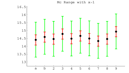
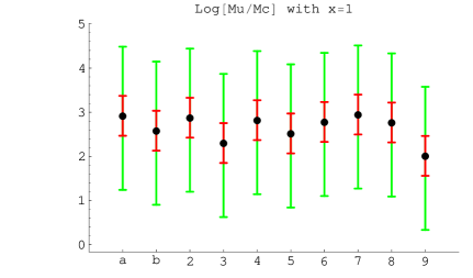
Figure 1: Compactification scale $\log_{10}(M_{c})$ and $\log_{10}(\Lambda/M_{c})$ ($M_{u}\equiv\Lambda$) versus SUSY spectrum, for $x=1$. The shorter error bars represent the parametric error dominated by the experimental uncertainty on $\alpha_{3}(m_{Z})$, the wider bars include the dominant source of error, the SO(10)-breaking brane terms $\delta_{i}^{(b)}\in\left[-1/2\pi,+1/2\pi\right]$.

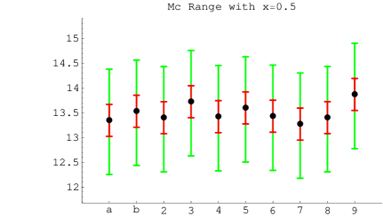
Figure 2: Compactification scale $\log_{10}(M_{c})$ and $\log_{10}(\Lambda/M_{c})$ ($M_{u}\equiv\Lambda$) versus SUSY spectrum for $x=1/2$. Error bars as in Fig. 1.

5 Proton lifetime

In our model proton decay is dominated by heavy gauge boson exchange. Indeed, dimension 5 operators arising through coloured higgsino exchange are forbidden by the U(1)_R R-symmetry of the 5D theory, only broken around the electroweak scale. We assume that, as in the MSSM, the R-parity subgroup of the U(1)_R symmetry remains an exact symmetry of the low-energy theory, thus prohibiting renormalizable baryon-violating operators as well. Therefore proton decay mainly proceeds through the exchange of the gauge bosons X and Y of the vector supermultiplet $V^{-}$ belonging to SO(10)$/$PS . Due to momentum conservation along the fifth dimension, preserved by bulk interaction terms, X and Y gauge bosons cannot couple to two zero modes of bulk hypermultiplets through minimal gauge interactions. They cannot minimally couple to zero modes on the PS brane either, since X and Y vanish at $y=\pi R/2$. The only zero modes that may have a minimal coupling to X and Y are those described by matter fields on the SO(10) brane. In our model matter fields are localized in the bulk or on the PS brane, see Table 2, and consequently dimension 6 baryon-violating minimal interactions are absent by construction. We stress that this conclusion is strictly related to our discussion of gauge coupling unification. As discussed in ref. [13], a correct next-to leading order gauge coupling unification requires the Higgs mechanism to take place on the PS brane. As a consequence, to properly break the unwanted SO(10) fermion mass relations, the simplest possibility is to accommodate the third generation on the PS brane and the other generations in the bulk, thus preventing proton decay via minimal coupling. The only possibility we are left with is to introduce non-minimal interactions of X, Y gauge bosons with matter fields. Considering the lowest possible dimension, there are two type of operators that violate the baryon number.

• Type I:

  Proton decay can arise from a derivative interaction localized on the PS brane:

  $${\cal L}_{I}=\frac{c}{\Lambda}\delta(y-\frac{\pi R}{2})\int d^{2}\theta d^{2}\bar{\theta}\ (\varphi)^{\dagger}\ (\nabla_{5}e^{2V})\ \varphi^{\prime}+h.c.$$ (64)

  where $\nabla_{5}=\partial_{5}+\Phi$ and $(\varphi,\varphi^{\prime})$ stands for any combination of $\psi_{3}$ and $\eta$.

• Type II

  Another contribution to proton decay can be originated by non-diagonal kinetic terms between two members of the doubling ($\psi_{i}$, $\psi_{i}^{\prime}$), $i=1,2$ of bulk fields. These operators are localized on the SO(10) symmetric brane:

  $${\cal L}_{II}=\frac{c^{\prime}}{\Lambda}\delta(y)\int d^{2}\theta d^{2}\bar{\theta}\ (\psi_{i})^{\dagger}(e^{2V})\ \psi^{\prime}_{i}+h.c.$$ (65)

The unknown constants $c$ and $c^{\prime}$ are expected to be of order one and are free parameters in the effective theory. Therefore proton lifetime cannot be calculated accurately and here we can only give a crude, order-of-magnitude, estimate, based on the leading operators (64, 65) of our model. After integrating out the super heavy gauge bosons X, Y ($M_{X,Y}=2M_{c}/\pi$), from Type I operators we obtain the four-fermion lagrangian:

$${\cal L}_{p}\sim\frac{c^{2}g_{U}^{2}}{2M_{X}^{2}}\frac{1}{\Lambda R}\left(a\overline{u^{c}_{3}}\gamma^{\mu}q_{3}\cdot\overline{e^{c}_{3}}\gamma_{\mu}q_{3}+b\overline{u^{c}_{3}}\gamma^{\mu}q_{3}\cdot\overline{d^{c}_{3}}\gamma_{\mu}l_{3}\right)~{}~{}~{},$$ (66)

where $a,b$ are dimensionless coefficient of order one and only the third generation is present [4]. From Type II operators we get

$${\cal L}_{p}\sim-\frac{(c^{\prime})^{2}g_{U}^{2}}{2M_{X}^{2}}\frac{1}{(\Lambda R)^{2}}\left(\overline{u^{c}_{i}}\gamma^{\mu}q_{i}\cdot\overline{e^{c}_{i}}\gamma_{\mu}q_{i}-2\overline{u^{c}_{i}}\gamma^{\mu}q_{i}\cdot\overline{d^{c}_{i}}\gamma_{\mu}l_{i}\right)~{}~{}~{},$$ (67)

where $i=1,2~{}$ [7].

Despite having the same dimension, the operators (66) and (67) have a different cut-off dependence. The derivative interaction (64) produces a relative enhancement of order $\Lambda R$. This can be easily understood by working in momentum space where the $1/n^{2}$ factor coming from the exchange of the $n$th KK mode is compensated by an $n^{2}$ factor coming from the interaction vertices. We are left with an unsuppressed sum over the KK modes, that can be regularized by cutting the upper limit of the sum at the KK mode whose mass exceeds the cut-off $\Lambda$. The sum gives approximately $\Lambda R$, the number of KK modes below the cut-off. However, the parametric enhancement of the operator (66) is not sufficient to overcome the huge suppression factor coming from the flavor mixing angles required to rotate third generation fields into fields relevant to proton decay. A detailed numerical analysis shows that the contribution from Type I operators is very suppressed and proton decay from this channel is beyond the possibilities of the next generation of experiments. We recall that the present experimental bound on the proton lifetime in the decay channel $e^{+}\pi^{0}$ is $\tau(p\to\pi^{0}e^{+})>5.4\times 10^{33}$ yr (90% C.L.), while the aimed for sensitivity of future experiments in the same channel is close to $10^{35}$ yr.

Type II operators are less suppressed but their contribution to proton decay is marginal. Qualitatively this can be understood from the fact that the mass scale suppressing dimension 6 operators in (67) is the combination $M_{X}\Lambda R\approx\Lambda$, which is much larger than the compactification scale $M_{X}$. The results for the dominant decay channels in this final case are shown in Fig. 3. We notice that the best values for the proton lifetime in the two channels displayed in Fig.(3) are not so different from the analogous values found in the SU(5) model analyzed in ref. [9]. The main difference deals with the theoretical error bar that in the present case covers about 4 orders of magnitude, while in the SU(5) case the uncertainty due to the unknown SU(5)-breaking brane contribution is much larger. The reduction in the theoretical uncertainty is here due to the fact that the amplitude is essentially controlled by the cut-off scale $\Lambda$, rather than the compactification scale as in SU(5), and $\Lambda$ is less sensitive than $M_{X}$ to the unknown SO(10) violating brane terms. Unfortunately the net result is that the possibility of seeing proton decay in this model and for these particular decay channels is even more disfavoured than in the SU(5) model.

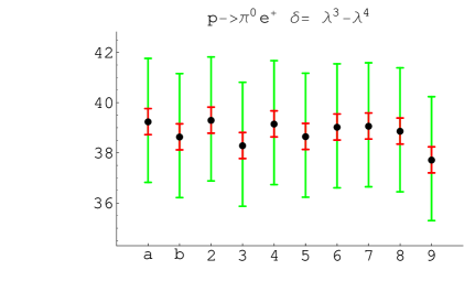
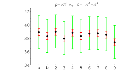
Figure 3: Proton lifetime versus SUSY spectrum for the dominant channels from Type II operators (we display the $\log_{10}$ of the lifetime in years). The smallest error bar is due to the experimental error from $\alpha_{3}$, while the biggest one derives from the theoretical uncertainties concerning the SO(10)- breaking brane terms $\delta_{i}^{(b)}\in\left[-1/2\pi,+1/2\pi\right]$. (For more details look at [9].)

6 Discussion

We have searched for a simple and semi-realistic realization of the SO(10) grand unified symmetry in the context of a 5D theory. To take advantage of the solution to the DT splitting problem offered by models with extra dimensions, it is sufficient to consider a single extra dimension and to reduce SO(10) down to the PS group by compactification on $S^{1}/Z_{2}$. The further breaking of the gauge symmetry down to the SM gauge group can be achieved through the ordinary Higgs mechanism taking place on the PS brane. In this note we have discussed in detail the fermion spectrum of the model with the hope of reproducing all the known features, at least at the level of orders of magnitude. Achieving a correct picture of fermion masses and mixing angles in an SO(10) GUT is not an easy task, not even at the level of a crude description. At variance with SU(5), where the theory with minimal field content can already accommodate a good first order approximation of the observed fermion spectrum, we cannot speak of a “minimal” SO(10) model. The reason is that in SO(10) with a minimal field content involving only the couplings $\psi_{i}\psi_{j}H_{10}$, the relation $M_{u}\propto M_{d}$ is completely wrong. Therefore, we need not only some mechanism to naturally produce hierarchies between Yukawa parameters, but also a certain degree of non-minimality.

In a 4D theory, hierarchies can be easily obtained by exploiting abelian flavour symmetries of the Froggatt-Nielsen (FN) type [22], and a variety of textures for fermion mass matrices in SU(5) GUTs have been successfully constructed [23] along these lines. Gauge theories formulated in more than four space-time dimensions offer alternative possibilities. Hierarchies between Yukawa couplings can be generated by the geometrical properties of the extra space, where matter fields may be localized in a variety of possible ways. In the case of a single extra dimension represented by an interval of length $L$, zero modes of bulk fields and brane fields enter Yukawa couplings with a relative normalization given by a factor $1/\sqrt{\Lambda L}$. Already in this simple case the observed hierarchy between fermion masses can be related to the hierarchy between the cut-off $\Lambda$ and the compactification scale $1/L$. Various attempts have been made in this direction based on SU(5) in 5D [9, 21]. Both in the case of abelian 4D flavour symmetries and in higher dimensional GUTs, it is not easy to accommodate realistic fermion masses if all matter fields of the same family belong to a single GUT representation, as it happens in SO(10). All fermions of a given generation tend to have similar Yukawa couplings and it is difficult to generate different hierarchical patterns in the different sectors.

To proceed towards a realistic model, some lessons can be drawn from the 4D case. One way to reproduce phenomenologically viable mass patterns of fermions in SO(10) is to depart from the “minimal” SO(10) Yukawa interactions by including higher representations of Higgs fields, which can correspond to new elementary degrees of freedom or to composite fields. In the ordinary 4D GUTs, this is a very popular approach and various realizations of Yukawa superpotentials, renormalizable or not, have been considered in the literature. In this direction, we find two kinds of realistic 4D SO(10) models. The first one is based on a relatively “compact” Higgs sector (for instance {16, $\overline{\text{\bf 16}}$, 45, 10}) and nonrenormalizable superpotentials [24]. In the second type of models the Higgs sector includes $H_{\overline{\text{126}}}$, a 126 SO(10) representation, and the minimal Yukawa interactions are modified by adding a new renormalizable contribution of the type $\psi_{i}\psi_{j}H_{\overline{\text{126}}}$ [25]. In both cases, an ad hoc pattern of Yukawa couplings is introduced in order to fit the experimental data. It should be said that in all SO(10) GUTs with extended Higgs sector the Higgs superpotential is quite complicated and obtaining the desired gauge symmetry breaking is not completely straightforward.

It is a general feature of 5D SUSY GUTs to have a minimal Higgs sector since the gauge symmetry is, at least in part, broken by compactification. Moreover a $U(1)_{R}$ symmetry is naturally present in 5D constructions and plays the important role of preventing too fast a proton decay. The allowed superpotential is rather restricted and the approach of extending it to include non-minimal terms related to higher Higgs representations is not as efficient as in the 4D case. Instead of dealing with extra Higgs fields, an alternative approach is to include extra matter multiplets, such as 10-plets of SO(10). In this way not all of the observed fermions in a given generation come from a single 16-plet, which gives rise to a much more flexible framework. For instance, SU(5)-like lopsided mass matrices for down quarks and charged leptons can be constructed and it is possible to better exploit flavour symmetries in SO(10) to correctly describe fermion masses and mixing angles [26].

This second approach can be incorporated in a SO(10) 5D construction and the present note provides a concrete realization of this idea. The hierarchy between the third generation and the other two is described by two small parameters, $\epsilon_{1}$ and $\epsilon_{2}$, arising because the third generation lives on the PS brane, while the other two live in the bulk. The relative suppression between second and third generation, $\epsilon_{2}$, is given by the geometrical normalization factor $\epsilon=1/\sqrt{\Lambda\pi R}$ of a flat zero mode relative to a brane field. The relative suppression between first and third generation, $\epsilon_{1}=\delta$, is slightly smaller than $\epsilon$, and arises from a zero mode with a non trivial profile in $y$. This setup is tuned to reproduce the mass hierarchy in the up quark sector, which fixes approximately $\epsilon\approx\lambda^{2}$ and $\delta\approx\lambda^{3}$. The down quark and the charged lepton masses are described by introducing a relative suppression $\epsilon_{u}$ between $(l,d^{c})$ and $(q,u^{c},e^{c},\nu^{c})$, within the third generation alone. Such a suppression is made possible by the fact that these two sectors do not belong to the same SO(10) irreducible representation. They are effectively embedded into a pair $16\oplus 10$, whose extra components acquire a very large mass. Order of magnitudes are correctly reproduced by taking $\epsilon_{u}\approx\lambda^{2}$.

Such a construction does not leave too much freedom to the neutrino sector. The heavy Majorana neutrino mass matrix and the Dirac neutrino mass matrix have the same order-of-magnitude structures of the up quark mass matrix and the charged lepton mass matrix, respectively. It is quite remarkable that through the see-saw mechanism they gives rise to a successful neutrino spectrum of normal hierarchy type with a large atmospheric mixing angle arising from the lopsided structure of the Dirac sector. The whole Yukawa sector is controlled by the VEVs of few multiplets: $H_{10}$, that breaks the electroweak symmetry, $\Sigma\oplus\bar{\Sigma}$, that breaks the PS symmetry down to the SM one and an SO(10) singlet $\theta$, that controls the absolute scale of neutrino masses. Early works based on 5D SO(10) can be found in [27, 28]. The authors of [27] combine a traditional U(1) flavour symmetry with the SO(10) GUT formulated in 5D. In this sense, the role of extra dimensions is marginal in order to reproduce their fermion mass pattern. Alternatively, in [28], the fermion mass hierarchy is generated by the breaking of the $U(1)_{X}$ subgroup of SO(10) in the bulk. The effect of this breaking is equivalent to introduce different bulk masses for matter hypermultiplets changing their bulk wave-function profile. However, in order to break $SO(10)\rightarrow SU(5)\times U(1)_{X}$, they have to introduce a 45 Higgs representation and, as in the first approach, an additional Dimopoulos-Wilczek mechanism is necessary to provide D-T splitting.

While proceeding in the construction of the Yukawa sector, our hope was that the peculiar setup we were defining could manifest in a direct and observable way at the level of proton decay. For this reason we have carefully analyzed proton decay in our model. There are no renormalizable interactions that violate baryon or lepton number and dimension five operators due to higgsino exchanged are forbidden. Baryon violating processes proceed through gauge vector boson exchange and are described by dimension six operators in the low energy theory. However, due to the specific localization of matter fields that emerges from the discussion of Yukawa couplings, there are no minimal couplings of fermions of first, second and third generations to the heavy gauge bosons X and Y that mediate proton decay. Non-minimal interactions are possible and we have listed the dominant ones. The main contribution to proton decay is described by a dimension 6 operator involving fermions of the first generation which is suppressed by the cut-off scale $\Lambda$, which replaces the heavy gauge boson masses $M_{X}$. As a result, unfortunately, the possibilities of detecting proton decay, even with future super-massive detectors, appear to be quite remote.

Acknowledgments We thank Arthur Hebecker for useful comments. This project is partially supported by the European Program MRTN-CT-2004-503369.

References

- [1] G. Altarelli, F. Feruglio and I. Masina, JHEP 0011 (2000) 040 [arXiv:hep-ph/0007254].
- [2] Y. Kawamura, Prog. Theor. Phys. 105 (2001) 999 [arXiv:hep-ph/0012125].
- [3] G. Altarelli and F. Feruglio, Phys. Lett. B 511 (2001) 257 [arXiv:hep-ph/0102301];
- [4] A. Hebecker and J. March-Russell, Phys. Lett. B 539 (2002) 119 [arXiv:hep-ph/0204037].
- [5] A. Hebecker and J. March-Russell, Nucl. Phys. B 613 (2001) 3. [arXiv:hep-ph/0106166].
- [6] L. J. Hall and Y. Nomura, Phys. Rev. D 64 (2001) 055003 [arXiv:hep-ph/0103125].
- [7] L. J. Hall and Y. Nomura, Phys. Rev. D 66 (2002) 075004 [arXiv:hep-ph/0205067].
- [8] L. Hall, J. March-Russell, T. Okui and D. R. Smith, JHEP 0409 (2004) 026 [arXiv:hep-ph/0108161].
- [9] M. L. Alciati, F. Feruglio, Y. Lin and A. Varagnolo, [arXiv:hep-ph/0501086].
- [10] T. Asaka, W. Buchmuller and L. Covi, Phys. Lett. B 523 (2001) 199 [arXiv:hep-ph/0108021]; L. J. Hall, Y. Nomura, T. Okui and D. R. Smith, Phys. Rev. D 65 (2002) 035008 [arXiv:hep-ph/0108071].
- [11] R. Dermisek and A. Mafi, Phys. Rev. D 65 (2002) 055002 [arXiv:hep-ph/0108139];
- [12] H. D. Kim and S. Raby, JHEP 0301 (2003) 056 [arXiv:hep-ph/0212348].
- [13] M. L. Alciati and Y. Lin, JHEP 0509 (2005) 061 [arXiv:hep-ph/0506130].
- [14] Y. Nomura, D. R. Smith and N. Weiner, Nucl. Phys. B 613 (2001) 147 [arXiv:hep-ph/0104041].
- [15] Y. Nomura and T. Yanagida, Phys. Rev. D 59 (1999) 017303 [arXiv:hep-ph/9807325].
- [16] G. Altarelli and F. Feruglio, New J. Phys. 6 (2004) 106 [arXiv:hep-ph/0405048].
- [17] B. C. Allanach et al., in Proc. of the APS/DPF/DPB Summer Study on the Future of Particle Physics (Snowmass 2001) ed. N. Graf, Eur. Phys. J. C 25 (2002) 113. [arXiv:hep-ph/0202233].
- [18] S. Eidelman et al. [Particle Data Group Collaboration], Phys. Lett. B 592, 1 (2004).
- [19] D. R. T. Jones, Phys. Rev. D 25 (1982) 581; M. B. Einhorn and D. R. T. Jones, Nucl. Phys. B 196 (1982) 475.
- [20] See for instance: Y. Yamada, Z. Phys. C 60 (1993) 83.
- [21] A. Hebecker and J. March-Russell, Phys. Lett. B 541, 338 (2002) [arXiv:hep-ph/0205143].
- [22] C. D. Froggatt and H. B. Nielsen, Nucl. Phys. B 147 (1979) 277.
- [23] Z. Berezhiani and Z. Tavartkiladze, Phys. Lett. B 396, 150 (1997), [arXiv:hep-ph/9611277]; G. Altarelli and F. Feruglio, Phys. Lett. B 451 (1999) 388, [arXiv:hep-ph/9812475]; Q. Shafi and Z. Tavartkiladze, Phys. Lett. B 451 (1999) 129, [arXiv:hep-ph/9901243]; G. Altarelli, F. Feruglio and I. Masina, JHEP 0011 (2000) 040, [arXiv:hep-ph/0007254].
- [24] S. M. Barr and S. Raby, Phys. Rev. Lett. 79 (1997) 4748 [arXiv:hep-ph/9705366]; C. H. Albright, K. S. Babu and S. M. Barr, Phys. Rev. Lett. 81 (1998) 1167 [arXiv:hep-ph/9802314]. K. S. Babu, J. C. Pati and F. Wilczek, Nucl. Phys. B 566 (2000) 3. [arXiv:hep-ph/9812538];
- [25] K. S. Babu and R. N. Mohapatra, Phys. Rev. Lett. 70 (1993) 2845 [arXiv:hep-ph/9209215]; B. Brahmachari and R. N. Mohapatra, Phys. Rev. D 58 (1998) 015001 [arXiv:hep-ph/9710371]; T. Fukuyama and N. Okada, JHEP 0211 (2002) 011 [arXiv:hep-ph/0205066]; C. S. Aulakh, B. Bajc, A. Melfo, G. Senjanovic and F. Vissani, Phys. Lett. B 588 (2004) 196 [arXiv:hep-ph/0306242].
- [26] Q. Shafi and Z. Tavartkiladze, Phys. Lett. B 487 (2000) 145, [arXiv:hep-ph/9910314]; N. Maekawa, Prog. Theor. Phys. 106 (2001) 401, [arXiv:hep-ph/0104200]; T. Asaka, Phys. Lett. B 562 (2003) 291 [arXiv:hep-ph/0304124].
- [27] Q. Shafi and Z. Tavartkiladze, Nucl. Phys. B 665 (2003) 469 [arXiv:hep-ph/0303150].
- [28] R. Kitano and T. j. Li, Phys. Rev. D 67 (2003) 116004 [arXiv:hep-ph/0302073].