hep-ph/yymmnnn

Little Higgs Dark Matter

Andreas Birkedal¹, Andrew Noble², Maxim Perelstein²,
and Andrew Spray²

¹ SCIPP, University of California, Santa Cruz, CA 95064
² Cornell Institute for High-Energy Phenomenology, Cornell University, Ithaca, NY 14853

The introduction of T parity dramatically improves the consistency of Little Higgs models with precision electroweak data, and renders the lightest T-odd particle (LTP) stable. In the Littlest Higgs model with T parity, the LTP is typically the T-odd heavy photon, which is weakly interacting and can play the role of dark matter. We analyze the relic abundance of the heavy photon, including its coannihilations with other T-odd particles, and map out the regions of the parameter space where it can account for the observed dark matter. We evaluate the prospects for direct and indirect discovery of the heavy photon dark matter. The direct detection rates are quite low and a substantial improvement in experimental sensitivity would be required for observation. A substantial flux of energetic gamma rays is produced in the annihilation of the heavy photons in the galactic halo. This flux can be observed by the GLAST telescope, and, if the distribution of dark matter in the halo is favorable, by ground-based telescope arrays such as VERITAS and HESS.

1 Introduction

It has now been firmly established that about 25% of the energy density in the universe exists in the form of nonrelativistic, non-baryonic, non-luminous matter, so called “dark matter” [1]. The microscopic composition of dark matter remains a mystery, but it is clear that it cannot consist of any elementary particles that have been directly observed in the laboratory so far. Many theories which extend the standard model (SM) of electroweak interactions contain new particles with the right properties to play the role of dark matter; perhaps the best known example is the lightest neutralino of supersymmetric (SUSY) models.

Recently, a new class of theories extending the SM at the TeV scale, “Little Higgs” (LH) models, has been proposed [2] (for reviews, see [3, 4]). The LH models contain a light (possibly composite) Higgs boson, as well as additional gauge bosons, fermions, and scalar particles at the TeV scale. The Higgs is a pseudo-Nambu-Goldstone boson, corresponding to a global symmetry spontaneously broken at a scale $f\sim 1$ TeV. The global symmetry is also broken explicitly by the gauge and Yukawa couplings of the Higgs. As a result of this breaking, the Higgs acquires a potential; however, the leading (one-loop, quadratically divergent) contribution to this potential vanishes due to the special “collective” nature of the explicit global symmetry breaking, and the lightness of the Higgs can be achieved without fine-tuning. The dynamics of the Higgs and other degrees of freedom relevant at the TeV scale is described by a non-linear sigma model (nlsm), valid up to the cutoff scale $\Lambda\sim 4\pi f\sim 10$ TeV. In particular, the Higgs mass term is dominated by a one-loop, logarithmically enhanced contribution from the top sector, which can be computed within the nlsm and shown to have the correct sign to trigger electroweak symmetry breaking, providing a simple and attractive explanation of this phenomenon. Above the cutoff scale, the model needs to be embedded in a more fundamental theory; however, for many phenomenological applications, including the analysis of this paper, the details of that theory are not relevant and the nlsm description suffices.

The Littlest Higgs model [2] is simple and economical, and it has been the focus of most phenomenological analyses to date [5]. Unfortunately, the model suffers from severe constraints from precision electroweak fits, due to the large corrections to low-energy observables from the tree-level exchanges of the non-SM TeV-scale gauge bosons and the small but non-vanishing weak-triplet Higgs vacuum expectation value (vev) [6]. To alleviate this difficulty, the symmetry of the theory can be enhanced to include a $Z_{2}$ discrete symmetry, named “T parity” [7]. In the Littlest Higgs model with T parity (LHT) [8], the non-SM gauge bosons and the triplet Higgs are T-odd, forbidding all tree-level corrections to precision electroweak observables. Loop corrections to precision electroweak observables in the LHT model were considered in [9], and the model was shown to give acceptable electroweak fits in large regions of parameter space compatible with naturalness.

An interesting side effect of T parity is that the lightest T-odd particle (LTP) is guaranteed to be stable. Analyzing the spectrum of the model, Hubisz and Meade [13] have argued that the LTP is likely to be the electricaly neutral, weakly interacting “heavy photon” (or, more precisely, the T-odd partner of the hypercharge gauge boson) $B_{H}$. This particle is an attractive dark matter candidate, and initial calculations [13] showed that its relic abundance is within the observed range for reasonable choices of model parameters. In this paper, we will present a somewhat more detailed relic density calculation, including the possibility of coannihilations between the $B_{H}$ and other T-odd particles. We will then discuss the prospects for direct and indirect detection of the heavy photon dark matter.

2 The Model

Our analysis will be performed within the framework of the Littlest Higgs model with T parity, which has recently been studied in Refs. [9, 13]. Let us briefly sketch the salient features of the model relevant here; for more details, see [9, 13] or the review article [4].

The model is based on an $SU(5)/SO(5)$ global symmetry breaking pattern; the Higgs doublet of the SM is identified with a subset of the Goldstone boson fields associated with this breaking. The symmetry breaking occurs at a scale $f\sim 1$ TeV. An $[SU(2)\times U(1)]^{2}$ subgroup of the $SU(5)$ is gauged; this is broken at the scale $f$ down to the diagonal subgroup, $SU(2)_{L}\times U(1)_{Y}$, identified with the SM electroweak gauge group. The extended gauge structure results in four additional gauge bosons at the TeV scale, $W^{\pm}_{H}$, $W^{3}_{H}$ and $B_{H}$.

T parity is an automorphism which exchanges the $\left[SU(2)\times U(1)\right]_{1}$ and $\left[SU(2)\times U(1)\right]_{2}$ gauge fields; under this transformation, the TeV-scale gauge bosons are odd, whereas the SM gauge bosons are even. The odd gauge bosons have masses

$$M(W_{H}^{a})\,\approx\,gf,~{}~{}~{}M\equiv M(B_{H})\,\approx\,\frac{g^{\prime}f}{\sqrt{5}}\approx 0.16f,$$ (1)

where $g$ and $g^{\prime}$ are the SM $SU(2)_{L}$ and $U(1)_{Y}$ gauge couplings, and the normalization of $f$ is the same as in Ref. [9]. (Electroweak symmetry breaking at the scale $v\ll f$ induces corrections to these formulas of order $v^{2}/f^{2}$.) The “heavy photon” $B_{H}$ is the lightest new gauge boson, and in fact is quite light compared to $f$. Since the masses of the other T-odd particles are generically of order $f$, we will assume that the $B_{H}$ is the lightest T-odd particle (LTP), and it will play the role of dark matter candidate. The only direct coupling of the heavy photon to the SM sector is via the Higgs, resulting in weak-strength cross sections for $B_{H}$ scattering into SM states. The heavy photon then provides yet another explicit example of a weakly interacting massive particle (WIMP) dark matter candidate, and it is not surprising that we will find reasonable regions of parameter space where it can account for all of the observed dark matter. For later convenience, we denote the mass of this particle by $M$. The range of the allowed values for this parameter is determined by the precision electroweak constraints, which put a lower bound on $f$, typically of about 600 GeV [9]. While there is no firm upper bound on $f$, we will assume $f\mathrel{\mathchoice{\lower 2.5pt\vbox{\halign{$\mathsurround 0pt\displaystyle\hfil#\hfil$\cr<\crcr\sim\crcr}}}{\lower 2.5pt\vbox{\halign{$\mathsurround 0pt\textstyle\hfil#\hfil$\cr<\crcr\sim\crcr}}}{\lower 2.5pt\vbox{\halign{$\mathsurround 0pt\scriptstyle\hfil#\hfil$\cr<\crcr\sim\crcr}}}{\lower 2.5pt\vbox{\halign{$\mathsurround 0pt\scriptscriptstyle\hfil#\hfil$\cr<\crcr\sim\crcr}}}}2$ TeV to avoid reintroducing fine tuning in the Higgs sector. Using Eq. (1), this corresponds to the WIMP masses in the range

$$100~{}{\rm GeV}\mathrel{\mathchoice{\lower 2.5pt\vbox{\halign{$\mathsurround 0pt\displaystyle\hfil#\hfil$\cr<\crcr\sim\crcr}}}{\lower 2.5pt\vbox{\halign{$\mathsurround 0pt\textstyle\hfil#\hfil$\cr<\crcr\sim\crcr}}}{\lower 2.5pt\vbox{\halign{$\mathsurround 0pt\scriptstyle\hfil#\hfil$\cr<\crcr\sim\crcr}}}{\lower 2.5pt\vbox{\halign{$\mathsurround 0pt\scriptscriptstyle\hfil#\hfil$\cr<\crcr\sim\crcr}}}}M\mathrel{\mathchoice{\lower 2.5pt\vbox{\halign{$\mathsurround 0pt\displaystyle\hfil#\hfil$\cr<\crcr\sim\crcr}}}{\lower 2.5pt\vbox{\halign{$\mathsurround 0pt\textstyle\hfil#\hfil$\cr<\crcr\sim\crcr}}}{\lower 2.5pt\vbox{\halign{$\mathsurround 0pt\scriptstyle\hfil#\hfil$\cr<\crcr\sim\crcr}}}{\lower 2.5pt\vbox{\halign{$\mathsurround 0pt\scriptscriptstyle\hfil#\hfil$\cr<\crcr\sim\crcr}}}}300~{}{\rm GeV}.$$ (2)

In the scalar sector, the model contains an additional T-odd weak-triplet field $\phi$, which has a mass of order $f$ and no vacuum expectation value. In the fermion sector, each SM doublet ($Q_{i}^{a}$ and $L_{i}$, where $a=1\ldots 3$ is a color index and $i=1\ldots 3$ is a generation index), acquires a T-odd partner, $\tilde{Q}_{i}^{a}$ and $\tilde{L}_{i}$. The masses of these particles are also free parameters, with the natural scale set by $f$. To avoid proliferation of parameters, we will assume a universal T-odd fermion mass $\tilde{M}$ for both lepton and quark partners; we will require $\tilde{M}>M$ to avoid charged or colored LTPs, and assume $\tilde{M}\mathrel{\mathchoice{\lower 2.5pt\vbox{\halign{$\mathsurround 0pt\displaystyle\hfil#\hfil$\cr>\crcr\sim\crcr}}}{\lower 2.5pt\vbox{\halign{$\mathsurround 0pt\textstyle\hfil#\hfil$\cr>\crcr\sim\crcr}}}{\lower 2.5pt\vbox{\halign{$\mathsurround 0pt\scriptstyle\hfil#\hfil$\cr>\crcr\sim\crcr}}}{\lower 2.5pt\vbox{\halign{$\mathsurround 0pt\scriptscriptstyle\hfil#\hfil$\cr>\crcr\sim\crcr}}}}300$ GeV, since otherwise the colored T-odd particles would have been detected in the squark searches at the Tevatron. In addition, non-observation of four-fermion operator corrections to SM processes such as $e^{+}e^{-}\rightarrow q\bar{q}$ places an upper bound on the T-odd fermion masses [9]:

$$\tilde{M}_{\rm TeV}<4.8\,f^{2}_{\rm TeV}\,,$$ (3)

where $\tilde{M}$ and $f$ are expressed in units of TeV. To cancel the one-loop quadratic divergence in the Higgs mass due to top loops, two additional new fermions are required in the top sector, the T-even $T_{+}$ and the T-odd $T_{-}$. Their masses are related by

$$M_{T_{+}}\,=\,M_{T_{-}}\,\left(1-\frac{m_{t}^{2}f^{2}}{v^{2}M_{T_{-}}^{2}}\right)^{-1/2},$$ (4)

so that there is just one additional independent parameter in this sector. We will choose it to be $M_{T_{-}}$, and assume $M_{T_{-}}>M$ to avoid a charged LTP. The couplings of the heavy photon $B_{H}$ which will be used in the calculations of this paper are summarized in Table 1.

$B_{H}^{\mu}B_{H}^{\nu}h$	$-\frac{i}{2}g^{\prime 2}vg^{\mu\nu}$
$B_{H}^{\mu}B_{H}^{\nu}hh$	$-\frac{i}{2}g^{\prime 2}g^{\mu\nu}$
$B_{H}^{\mu}\tilde{Q}_{i}^{a}Q_{j}^{b}$	$i\tilde{Y}\,g^{\prime}\gamma^{\mu}P_{L}\delta_{ij}\delta^{ab}$
$B_{H}^{\mu}\tilde{L}_{i}L_{i}$	$i\tilde{Y}\,g^{\prime}\gamma^{\mu}P_{L}\delta_{ij}$
$B_{H}^{\mu}T_{-}t$	$i\left(\frac{2}{5}\right)\,g^{\prime}\gamma^{\mu}\sin\alpha\left(\sin\alpha\frac{v}{f}P_{L}+P_{R}\right)$

Table 1: Interaction vertices involving the heavy photon $B_{H}$ that appear in the calculations of this paper. Here $\alpha=\cos^{-1}(M_{T_{-}}/M_{T_{+}})$, and $\tilde{Y}=1/10$.

3 Relic Density Calculation

Figure 1: The leading $2\leftrightarrow 2$ processes which maintain the heavy photon in equilibrium with the rest of the cosmic fluid at high temperatures.

In the early universe, the heavy photons are in equilibrium with the rest of the cosmic fluid. In the simplest case of generic (non-degenerate) T-odd particle mass spectrum, the equilibrium is maintained via the heavy photon pair-annihilation and pair-creation reactions; the leading $2\leftrightarrow 2$ processes that contribute are shown in Fig. 1. The present relic abundance of heavy photons is determined by the behavior of pair-annihilation rates in the non-relativistic limit, namely, by the sum of the quantities

$$a(X)=\lim_{u\rightarrow 0}\sigma(B_{H}B_{H}\rightarrow X)u,$$ (5)

over all possible final states $X$. Here, $u$ is the relative velocity of the annihilating particles. Note that, unlike the bino-like neutralinos typically predicted by the constrained minimal supersymmetric standard model (cMSSM), the $s$-wave annihilation of the heavy photons is unsuppressed: in the language of Ref. [16], the heavy photons are “$s$ annihilators”, analogous to the Kaluza-Klein photons of the “universal extra dimensions” (UED) model [17, 18]. It is straightforward to compute $a(X)$ using the Feynman rules in Table 1. We obtain

$$a(W^{+}W^{-}) = \frac{2\pi\alpha^{2}}{3\cos^{4}\theta_{W}}\,\frac{M^{2}}{(4M^{2}-m_{h}^{2})^{2}+m_{h}^{2}\Gamma_{h}^{2}}\,\left(1-\mu_{w}+\frac{3}{4}\mu_{w}^{2}\right)\sqrt{1-\mu_{w}}\,,$$

$$a(ZZ) = \frac{\pi\alpha^{2}}{3\cos^{4}\theta_{W}}\,\frac{M^{2}}{(4M^{2}-m_{h}^{2})^{2}+m_{h}^{2}\Gamma_{h}^{2}}\,\left(1-\mu_{z}+\frac{3}{4}\mu_{z}^{2}\right)\sqrt{1-\mu_{z}}\,,$$

where $\mu_{i}=m_{i}^{2}/M^{2}$, $\theta_{W}$ is the SM weak mixing angle, and $m_{h}$ and $\Gamma_{h}$ are the mass and the width of the SM Higgs boson. If $M>m_{t}$, the LTPs can also annihilate into pairs of top quarks; ignoring the contribution from the $t$- and $u$-channel $T_{-}$ exchanges, we obtain

$$a(t\bar{t})\,=\,\frac{\pi\alpha^{2}}{\cos^{4}\theta_{W}}\,\frac{M^{2}}{(4M^{2}-m_{h}^{2})^{2}+m_{h}^{2}\Gamma_{h}^{2}}\,\mu_{t}(1-\mu_{t})^{3/2}\,.$$ (7)

If $M>m_{h}$, annihilation into a pair of Higgs bosons is possible, with the cross section

$$a(hh)=\frac{\pi\alpha^{2}M^{2}}{2\cos^{4}\theta_{W}}\,\left[\frac{\mu_{h}(1+\mu_{h}/8)}{(4M^{2}-m_{h}^{2})^{2}+m_{h}^{2}\Gamma_{h}^{2}}\,+\,\frac{1}{24M^{4}}\right]\,\sqrt{1-\mu_{h}}.$$ (8)

Finally, LTPs can also annihilate into light SM fermions via $t$-channel exchanges of the T-odd fermions; this channel was not included in the analysis of Ref. [13]. For a fermion $f$ ($f=\ell^{\pm},\nu,u,d$) we obtain

$$a(f\bar{f})\,=\,\frac{16\pi\alpha^{2}\tilde{Y}^{4}N_{c}^{f}}{9\cos^{4}\theta_{W}}\,\frac{M^{2}}{(M^{2}+\tilde{M}^{2})^{2}}\,,$$ (9)

where $N_{c}^{f}=1$ for leptons and 3 for quarks, and $\tilde{Y}=1/10$ is the $B_{H}f\tilde{f}$ coupling in units of $g^{\prime}$. Because of the small value of $\tilde{Y}$, the annihilation into light fermions is strongly suppressed, even for relatively small values of $\tilde{M}$. The WMAP collaboration data [19] provides a precise determination of the present dark matter abundance: at two-sigma level,

$$\Omega_{\rm dm}h^{2}=0.111\pm 0.018.$$ (10)

For $s$ annihilators, this translates into a determination of the quantity $a\equiv\sum_{X}a(X)$: $a=0.8\pm 0.1$ pb. (The precise central value of $a$ depends on the WIMP mass; however, this dependence is very mild, see Fig. 1 of Ref. [16].) Using this constraint and the above formulas, it is straightforward to map out the regions of the model parameter space where the heavy photons can account for all of the observed dark matter. The results are consistent with the updated analysis of Hubisz and Meade, see Fig. 3 of Ref. [13]. For given $m_{h}$, there are two values of $M$ which result in the correct relic density. There is one solution on either side of the Higgs resonance. For WIMP masses in the interesting range, Eq. (2), these can be approximated by simple analytic expressions:

$$m_{h}\approx 24+2.38M,~{}~{}~{}{\rm or}~{}~{}~{}m_{h}\approx-83+1.89M,$$ (11)

where $M$ and $m_{h}$ are in units of GeV. We will refer to these solutions as “low” and “high”, respectively. The analytic expressions (11) reproduce the values of $M$ and $m_{h}$ consistent with the WMAP central value of $\Omega_{\rm dm}h^{2}$ with an error of at most a few GeV throughout the interesting parameter range. This accuracy will be sufficient for the analysis of detection prospects in Sections 4 and 5.

Throughout the parameter space consistent with the WMAP value of the present dark matter density, the dominant heavy photon annihilation channels are $W^{+}W^{-}$ and $ZZ$; the $t\bar{t}$ channel contributes at most about 5% of the total annihilation cross section, while the $hh$ final state is always kinematically forbidden. Moreover, the ratio of the $W^{+}W^{-}$ and $ZZ$ contributions is approximately 2:1, as is evident from Eqs. (LABEL:wz), so that $a(W^{+}W^{-})\approx 0.53$ pb, $a(ZZ)\approx 0.27$ pb throughout the parameter space. Since $B_{H}$ is an $s$-annihilator, the same cross sections govern the rate of heavy photon annihilation in the galactic halo, which in turn determines the fluxes relevant for indirect detection, see Section 5.

If some of the T-odd particles are approximately degenerate in mass with the heavy photon, the simple analysis above is no longer applicable, since coannihilation reactions between $B_{H}$ and other states significantly affect the relic abundance. In the LHT model, the masses of the T-odd weak gauge bosons $W_{H}$ and the triplet scalar $\phi$ are predicted unambiguously once the scale $f$ and the Higgs mass $m_{h}$ are fixed; these particles are always much heavier than the $B_{H}$ and their effect is negligible. On the other hand, the common mass scale of the T-odd leptons and quarks $\tilde{M}$ is a free parameter, and for $M\sim\tilde{M}$ the coannihilations between these states and the $B_{H}$ can be important. We have performed a more detailed analysis of the $B_{H}$ relic density, taking this possibility into account.

In the presence of coannihilations, the abundance calculation requires solving a system of coupled Boltzmann equations. We approached this problem numerically. The interactions of the LHT model were incorporated in the CalcHEP package [20], which was used to compute the scattering matrix elements for the appropriate processes. The rest of the calculation was performed using the DM++ package, recently recently developed by one of us (AB). The package first uses the matrix elements to compute the thermal averages $\left<\sigma u\right>$, which determine the reaction rates entering the Boltzmann equation. Then, the freeze-out temperature of the dark matter is determined iteratively, using the Turner-Scherrer approximation [23]. Finally, the integral of $\left<\sigma u\right>$ from freeze-out to present day (usually called $J\left(x_{F}\right)$ in the literature) is evaluated, providing the relic abundance.

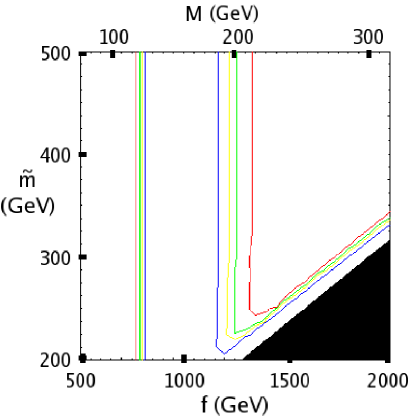
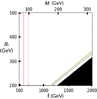
Figure 2: The contours of constant present abundance of the heavy photon LTP, $\Omega_{\rm LTP}h^{2}$, in the $M-\tilde{M}$ plane. The Higgs mass is taken to be 300 GeV (left panel) and 120 GeV (right panel). The red and green contours correspond to the upper and lower bounds from WMAP, Eq. (10), assuming that the LTP makes up all of dark matter. The yellow and blue lines correspond to the LTP contributing 50% and 70%, respectively, of the measured dark matter density. The shaded region corresponds to a charged and/or colored LTP.

The results of this analysis are illustrated by Figure 2, which shows the contours of constant heavy photon relic density in the $f-\tilde{M}$ (or, equivalently, $M-\tilde{M}$) plane. The typical situation for a heavy Higgs is shown in the left panel ($m_{h}=300$ GeV). There are two regions in which the heavy photon can account for the observed dark matter:

• The two vertical pair-annihilation bands, where the coannihilation processes are unimportant. The heavy photon abundance in these regions is independent of $\tilde{M}$. The bands appear on either side of the $s$-channel Higgs resonance dominating the pair-annihilation processes, corresponding to the “high” and “low” solutions of Eq. (11). (The bands are analogous to the “Higgs funnel” region in the cMSSM.)

• The coannihilation tail, where the heavy photon abundance is predominantly set by coannihilation processes. Since the T-odd fermions are assumed to be degenerate, all of them participate in the coannihilation reactions. The location and shape of this feature are similar to the tau coannihilation tail in cMSSM.

As the Higgs mass is decreased, the pair-annihilation bands appear for lower WIMP masses, and for light Higgs (115–150 GeV) the “low” band disappears, since the required values of $f$ are already ruled out by data. The “high” band persists until the Higgs mass is close to the current experimental bound. To illustrate this, consider the right panel of Fig. 2, where $m_{h}=120$ GeV. The band between the two red lines ($90\mathrel{\mathchoice{\lower 2.5pt\vbox{\halign{$\mathsurround 0pt\displaystyle\hfil#\hfil$\cr<\crcr\sim\crcr}}}{\lower 2.5pt\vbox{\halign{$\mathsurround 0pt\textstyle\hfil#\hfil$\cr<\crcr\sim\crcr}}}{\lower 2.5pt\vbox{\halign{$\mathsurround 0pt\scriptstyle\hfil#\hfil$\cr<\crcr\sim\crcr}}}{\lower 2.5pt\vbox{\halign{$\mathsurround 0pt\scriptscriptstyle\hfil#\hfil$\cr<\crcr\sim\crcr}}}}M\mathrel{\mathchoice{\lower 2.5pt\vbox{\halign{$\mathsurround 0pt\displaystyle\hfil#\hfil$\cr<\crcr\sim\crcr}}}{\lower 2.5pt\vbox{\halign{$\mathsurround 0pt\textstyle\hfil#\hfil$\cr<\crcr\sim\crcr}}}{\lower 2.5pt\vbox{\halign{$\mathsurround 0pt\scriptstyle\hfil#\hfil$\cr<\crcr\sim\crcr}}}{\lower 2.5pt\vbox{\halign{$\mathsurround 0pt\scriptscriptstyle\hfil#\hfil$\cr<\crcr\sim\crcr}}}}100$ GeV) is allowed. Note that the behavior of the relic density as a function of $M$ within this band is non-trivial: The relic density first drops with increasing $M$ due to the fact that the threshold for the reaction $B_{H}B_{H}\rightarrow ZZ$ is passed. It then bottoms out at a value consistent with the measured $\Omega_{\rm dm}h^{2}$, and begins increasing as increasing $M$ further takes the center-of-mass energy away from the Higgs resonance, suppressing annihilation. Clearly, this situation is quite non-generic, and for somewhat higher $m_{h}$ the $Z$ threshold becomes irrelevant and relic density is a uniformly increasing function of $M$ in the “high” band. The coannihilation tail is present for low as well as high values of $m_{h}$. The tail can be described by a simple analytic formula

$$\tilde{M}\approx M+20~{}{\rm GeV},$$ (12)

which is approximately independent of the Higgs mass.

It should be noted that the remaining free parameter of our model, the mass of the second T-odd top quark $M_{T_{-}}$, was fixed to be equal to $f$, so that $M_{T_{-}}\gg M$ and this particle did not have an effect on the $B_{H}$ relic abundance. We expect that a second coannihilation tail appears when $M_{T_{-}}\sim M$; the structure should be very similar to the one found above, with slight numerical differences due to smaller multiplicity of the coannihilating states.

4 Direct Detection

Direct dark matter detection experiments attempt to observe the recoil energy transfered to a target nucleus in an elastic collision with a WIMP. The null result of the current experiments places an upper bound on the cross section of elastic WIMP-nucleon scattering. In this section, we will discuss the implications of this bound for the LHT dark matter, and prospects for future discovery.

Figure 3: The leading processes which contribute to the heavy photon–nucleon elastic scattering cross section relevant for direct dark matter detection experiments.

The elastic scattering of the heavy photon on a nucleus receives contributions from several processes shown in Fig. 3. Consider first the scattering off gluons, which occurs via the Higgs exchange diagram (a). The Higgs-gluon coupling arises predominantly via a top quark loop, and has the form [24]

$${\cal L}_{hgg}\,=\,\frac{\alpha_{s}}{12\pi v}\,hG^{a}_{\mu\nu}G^{a\mu\nu}.$$ (13)

where $v=246$ GeV is the Higgs vev, and $G^{a}_{\mu\nu}$ is the color field strength. The halo WIMPs are highly nonrelativistic ($\beta\sim 10^{-3}$), and the momentum transfer in the reaction at hand is negligible compared to $m_{h}$. The WIMP-gluon interaction can then be described by an effective operator

$$\frac{\alpha_{s}\alpha}{6\cos^{2}\theta_{W}}\frac{1}{m_{h}^{2}}B_{{\rm H}\alpha}B^{\alpha}_{\rm H}\,G^{a}_{\mu\nu}G^{a\mu\nu}.$$ (14)

In the chiral limit, the matrix element $\left<n|G^{2}|n\right>$ can be related to the nucleon mass $m_{n}$ [24], leading to an effective WIMP-nucleon vertex of the form

$${\cal L}_{\rm eff}\,=\,\frac{e^{2}}{27\cos^{2}\theta_{W}}\frac{m_{n}}{m_{h}^{2}}\,B_{{\rm H}\alpha}B^{\alpha}_{\rm H}\,\bar{\Psi}_{n}\Psi_{n},$$ (15)

where $\Psi_{n}$ is the nucleon (neutron or proton) field. It is clear that this interaction only contributes to the spin-independent (SI) part of the WIMP-nucleon scattering cross section. Neglecting other contributions to the SI cross section (which, as we will argue below, are expected to be subdominant), we obtain

$$\sigma_{\rm SI}\,=\,\frac{4\pi\alpha^{2}}{729\cos^{4}\theta_{W}}\,\frac{m_{n}^{4}}{m_{h}^{4}}\,\frac{1}{(M+m_{n})^{2}},$$ (16)

for both neutrons and protons. Since the scattering off nucleons in a given nucleus is coherent and the matrix elements for neutrons and protons are identical, the SI cross section for scattering off a nucleus of mass $m_{N}$ is simply obtained from Eq. (16) by a substitution $m_{n}\rightarrow m_{N}$.

The interaction of WIMPs with quarks is dominated by the T-odd quark exchange diagrams, see Fig. 3 (b) and (c). (The Higgs exchange diagrams are suppressed due to small Yukawa couplings of quarks. In fact, it is well known that the Higgs-nucleon interaction is dominated by the Higgs-gluon coupling considered above.) The scattering amplitude is given by

$$-i\frac{e^{2}\tilde{Y}^{2}}{\cos^{2}\theta_{W}}\varepsilon_{\mu}^{\ast}(p_{3})\varepsilon_{\nu}(p_{1})\,\,\bar{u}(p_{4})\!\left[\frac{\gamma^{\mu}\!\not{\!k}_{1}\gamma^{\nu}}{k_{1}^{2}-\tilde{M}^{2}}+\frac{\gamma^{\nu}\!\not{\!k}_{2}\gamma^{\mu}}{k_{2}^{2}-\tilde{M}^{2}}\right]\!P_{L}\,u(p_{2})\ ,$$ (17)

where $k_{1}=p_{1}+p_{2}$, $k_{2}=p_{2}-p_{3}$. The $q\tilde{q}B_{H}$ coupling is flavor-independent, $\tilde{Y}=1/10$, and the expression (17) is valid for every quark species. The amplitude contains two important physical scales: the weak scale, $M\sim\tilde{M}\sim 100$ GeV, and the QCD scale, $\Lambda_{\rm QCD}\sim 100$ MeV, which represents the typical energy and momentum of the quarks bound inside a stationary nucleus and, by a coincidence, the spatial momenta of the halo WIMPs: $|{\bf p}|_{1,3}\sim\beta M\sim\Lambda_{\rm QCD}$. We will work to leading order in the ratio of these two scales. In this approximation, $k_{1}\approx-k_{2}\approx(M,{\mathbf{0}})$, and the heavy photon polarization vectors are purely spatial, $\varepsilon^{\mu}(p_{1,3})=(0,\varepsilon_{1,3})$. The amplitude takes the form

$$\frac{e^{2}\tilde{Y}^{2}}{\cos^{2}\theta_{W}}\,\frac{M}{M^{2}-\tilde{M}^{2}}\,\epsilon_{ijk}\varepsilon_{1}^{i}\varepsilon^{j}_{3}\bar{u}_{4}\gamma^{k}(1-\gamma^{5})u_{2}\,,$$ (18)

corresponding to the coupling of the $B_{H}$ spin with the vector and axial-vector quark currents. The axial current interaction corresponds to the coupling between the WIMP and quark spins, and gives rise to the spin-dependent (SD) part of the WIMP-nucleus scattering cross section. By the Wigner-Eckardt theorem, the quark axial current can be replaced by the nuclear spin operator $s^{\mu}_{N}$:

$$\left<N|\bar{q}\gamma^{\mu}\gamma^{5}q|N\right>\,=\,2s^{\mu}_{N}\lambda_{q}.$$ (19)

For a nucleus of spin $J_{N}$, the coefficients are given by

$$\lambda_{q}=\Delta q_{p}\frac{\left<S_{p}\right>}{J_{N}}+\Delta q_{n}\frac{\left<S_{n}\right>}{J_{N}},$$ (20)

where $\left<S_{p,n}\right>/J_{N}$ is the fraction of the total nuclear spin carried by protons and neutrons, respectively, and the quantities $\Delta q_{n}$ can be extracted from deep inelastic scattering data. We will use $\Delta u_{p}=\Delta d_{n}=0.78\pm 0.02$, $\Delta d_{p}=\Delta u_{n}=-0.48\pm 0.02$, $\Delta s_{n}=\Delta s_{p}=-0.15\pm 0.02$ [25]. The effective WIMP-nucleus spin-spin interaction can then be written as

$$\frac{2e^{2}\tilde{Y}^{2}M}{\cos^{2}\theta_{W}(M^{2}-\tilde{M}^{2})}\,\epsilon_{ijk}B_{H}^{i}B_{H}^{j}\bar{\Psi}_{N}s^{k}_{N}\Psi_{N}\,\sum_{q=u,d,s}\lambda_{q},$$ (21)

yielding the SD cross section

$$\sigma_{\rm SD}\,=\,\frac{16\pi\alpha^{2}\tilde{Y}^{4}}{3\cos^{4}\theta_{W}}\frac{m_{N}^{2}}{(M+m_{N})^{2}}\,\frac{M^{2}}{(M^{2}-\tilde{M}^{2})^{2}}\,J_{N}(J_{N}+1)\left(\sum_{q=u,d,s}\lambda_{q}\right)^{2}.$$ (22)

Now, consider the part of the amplitude (18) involving the quark vector current. Since the current is conserved, the contributions of each valence quark in a nucleon add coherently, and sea quarks do not contribute. The resulting WIMP-nucleon coupling is

$$\frac{3e^{2}\tilde{Y}^{2}M}{\cos^{2}\theta_{W}(M^{2}-\tilde{M}^{2})}\,\epsilon_{ijk}B_{H}^{i}B_{H}^{j}\bar{\Psi}_{n}\gamma^{k}\Psi_{n}\,.$$ (23)

This interaction is suppressed in the nonrelativistic limit, since $\bar{u}_{n}\gamma^{k}u_{n}\sim v_{n}^{k}$. In fact, it is of the same order as other contributions to the WIMP-quark scattering amplitude, suppressed by WIMP velocities or powers of $\Lambda_{\rm QCD}/M$, which were neglected in our analysis. Therefore, its effect will be neglected.

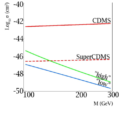
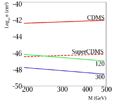
Figure 4: The spin-independent (SI) WIMP-nucleon elastic scattering cross section in the pair-annihilation bands (left panel) and in the coannihilation region, for two values of $m_{h}$, 120 and 300 GeV (right panel). The present [26] and projected [27] sensitivities of the CDMS experiment are also shown.

It should be noted that the SI interaction in Eq. (15), is parametrically suppressed with respect to the leading SD coupling, Eq. (21), by a factor of $m_{N}/m_{h}\sim\Lambda_{\rm QCD}/M$, and is formally of the same order as the contributions to the WIMP-quark interaction that were neglected in our analysis. Since the neglected terms contribute to the SI as well as SD interactions, one may question the validity of the SI cross section obtained in Eq. (16). Note, however, that the WIMP-quark interactions are additionally suppressed by a factor of $\tilde{Y}^{2}=0.01$, not present in the WIMP-gluon couplings. Thus, while of the same order as (15) in terms of power counting, the neglected SI corrections from WIMP-quark interactions are expected to be numerically small. One interesting potential exception occurs in the coannihilation region, where the $\tilde{Y}$ suppression could be compensated by the factor of $\tilde{M}-M\ll M$ in the propagator, and the WIMP-quark interactions could provide a significant correction to Eq. (16). A detailed analysis of this issue is reserved for future study.

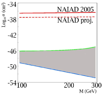
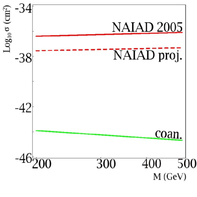
Figure 5: The spin-dependent (SD) WIMP-proton elastic scattering cross section in the pair-annihilation bands (left panel) and in the coannihilation region (right panel). In the pair-annihilation bands, the scale $\tilde{M}$ is allowed to vary between 350 GeV and the upper bound given in Eq. (3). The present [28] and projected [29] sensitivities of the NAIAD experiment are also shown.

The SI elastic WIMP-nucleon scattering cross sections expected in the LHT models are plotted in Fig. 4, along with the current bound from the CDMS collaboration [26] (solid red lines) and the projected future sensitivity of SuperCDMS, stage C [27] (dashed red lines). We assume that the heavy photons account for all of the observed dark matter, and the two panels correspond to the two regions of parameter space which satisfy this constraint. The left panel shows the cross section expected in the pair-annihilation bands, with the two lines corresponding to the high and low solutions in Eq. (11). The right panel shows the cross section expected in the coannihilation tail for two values of the Higgs mass, 120 GeV and 300 GeV. The two lines can be thought of as the upper and lower bounds on the expected cross section. While the predicted cross sections are two-three orders of magnitude below the present sensitivity, the expected improvements of the CDMS experiments will allow it to begin probing the interesting regions of the model parameter space in both pair-annihilation and coannihilation regions.

Fig. 5 shows the spin-dependent cross sections predicted by the LHT model, along with the current bound from the NAIAD experiment [28] and its projected sensitivity [29]. In the pair-annihilation bands, the scale $\tilde{M}$ is allowed to vary between 350 GeV and the upper bound given in Eq. (3). (Recall that for a given value of $M$, the scale $f$ is fixed unambiguously by Eq. (1).) Unfortunately, the predicted SD cross sections are several orders of magnitude below the NAIAD sensitivity.

5 Indirect Detection via Anomalous Gamma Rays

As discussed in Section 3, WIMP annihilation processes have to occur with approximately weak-scale cross sections to ensure that the relic abundance of WIMPs is consistent with observations. Since the heavy photons of the LHT model are $s$-annihilators, their annihilation rates are approximately velocity-independent in the nonrelativistic regime. This implies that the WIMPs collected, for example, in galactic halos, have a substantial probability to pair-annihilate, resulting in anomalous high-energy cosmic rays which could be distinguished from astrophysical backgrounds. In particular, high-energy gamma rays (photons) and positrons are considered to be the most promising experimental signatures. The gamma ray signal is particularly interesting because the gamma rays in the relevant energy range travel over galactic scales with no scattering, so that if the signal is observed, information about the WIMP (e.g. its mass) could be extracted from the spectrum. In this section, we will compute the gamma ray fluxes predicted by the LHT model, and evaluate their observability.

There are three principal mechanisms by which hard photons can be produced in WIMP annihilation:

• Monochromatic photons produced via direct annihilation into a two body final state ($\gamma\gamma,h\gamma$ or $Z\gamma$);

• Photons radiated in the process of hadronization and fragmentation of strongly interacting particles produced either directly in WIMP annihilation (e.g. $B_{H}B_{H}\rightarrow q\bar{q}$) or in hadronic decays of the primary annihilation products (e.g. $B_{H}B_{H}\rightarrow ZZ$ followed by $Z\rightarrow q\bar{q}$);

• Photons produced via radiation from a final state charged particle.

Let us consider each of these mechanisms in turn in the LHT model.

Figure 6: The diagrams which dominate the monochromatic photon pair-production in the $B_{H}$ annihilation in the galactic halo.

WIMPs being electrically neutral, production of monochromatic photons can only occur at loop level. In this paper, we will concentrate on the $\gamma\gamma$ final state, postponing the analysis of the $Z\gamma$ and $h\gamma$ channels for future work. (The photons produced in these reactions are separated in energy from the $\gamma\gamma$ photons due to non-zero masses of the $Z$ and the Higgs.) The $B_{H}B_{H}\rightarrow\gamma\gamma$ process is dominated by the one-loop diagrams inducing the effective $h\gamma\gamma$ vertex, see Fig. 6. The corresponding cross section can be easily evaluated using the well-known formulas for the Higgs boson partial widths:

$$\sigma_{\gamma\gamma}u\equiv\sigma\left(B_{H}B_{H}\rightarrow\gamma\gamma\right)u=\frac{g^{\prime 4}v^{2}}{72M^{4}}\,\frac{s^{2}-4sM^{2}+12M^{4}}{(s-m_{h}^{2})^{2}+m_{h}^{2}\Gamma_{h}^{2}}\,\frac{\hat{\Gamma}\left(h\rightarrow V_{1}V_{2}\right)}{\sqrt{s}},$$ (24)

where $u$ is the relative velocity of the annihilating WIMPs, and $s\approx 4M^{2}$ in the non-relativistic regime relevant for the galactic WIMP annihilation. The hat on $\Gamma$ indicates that the substitution $m_{h}\rightarrow\sqrt{s}$ should be performed in the standard expressions for on-shell Higgs decays [32, 33], and the loops of new particles present in the LHT model should be included. We obtain

$$\hat{\Gamma}(h\rightarrow\gamma\gamma)\,=\,\frac{\alpha^{2}g^{2}}{1024\pi^{3}}\frac{s^{3/2}}{m_{W}^{2}}\,\Bigl{|}{\cal A}_{1}+{\cal A}_{1/2}+{\cal A}_{0}\Bigr{|}^{2},$$ (25)

where ${\cal A}_{s}$ denotes the contribution from loops of particles of spin $s$. These contributions are given by

$${\cal A}_{1} = \sum_{i}c_{i}Q_{i}^{2}\frac{\tau_{W}}{\tau_{i}}F_{1}(\tau_{i});$$

$${\cal A}_{1/2} = \sum_{i}\frac{\sqrt{2}Q_{i}^{2}y_{i}}{g}\frac{\tau_{W}^{1/2}}{\tau_{i}^{1/2}}F_{1/2}(\tau_{i});$$

$${\cal A}_{0} = \sum_{i}\frac{2Q_{i}^{2}\lambda_{i}}{g^{2}}\frac{\tau_{W}}{\tau_{i}}F_{0}(\tau_{i}),$$ (26)

where the sums run over all the charged particles of a given spin, and implicitly include summations over colors and other quantum numbers where necessary. The particles in the sums have masses $m_{i}$ and electric charges (in units of the electron charge) $Q_{i}$; their trilinear couplings to the Higgs boson are given by $\lambda_{i}v$, $y_{i}/\sqrt{2}$, and $c_{i}gM_{W}\eta^{\mu\nu}$, for particles of spin 0, 1/2, and 1, respectively. (With these normalization choices, $c_{i}=1$ for the SM $W^{\pm}$, and $y_{i}$’s are the usual Yukawas for the SM fermions.) We have also defined $\tau_{i}=4m_{i}^{2}/s$. The functions $F_{s}(\tau)$ are given by

$$F_{1}(\tau) = 2+3\tau+3\tau\left(2-\tau\right)f(\tau),$$

$$F_{1/2}(\tau) = -2\tau\left(1+\left(1-\tau\right)f(\tau)\right),$$

$$F_{0}(\tau) = \tau\left(1-\tau f(\tau)\right),$$ (27)

where

$$f(\tau) = \left[\sin^{-1}\left(\sqrt{\frac{1}{\tau}}\right)\right]^{2}~{}~{}{\rm if}~{}\tau>1,$$ (28)

$$-\frac{1}{4}\left[\log\left(\frac{1+\sqrt{1-\tau}}{1-\sqrt{1-\tau}}\right)-i\pi\right]^{2}~{}{\rm if}~{}\tau<1.$$

Using these expressions, we find that the contributions of the T-odd states are subdominant compared to the SM loops. The contributions of the T-odd fermion loops and the T-even heavy top loop are suppressed because their coupling to the Higgs is of order $v^{2}/f^{2}$. The contributions of charged T-odd heavy gauge bosons and scalars are suppressed due to their large masses, of order $f$. The deviation of the effective $h\gamma\gamma$ coupling from its Standard Model value due to these states is of order a few per cent. Given the much larger astrophysical uncertanties inherent in the anomalous photon flux predictions, we will ignore these effects in our analysis.

The monochromatic flux due to the $\gamma\gamma$ final state, observed by a telescope with a line of sight parametrized by $\Psi=(\theta,\varphi)$ and a field of view $\Delta\Omega$ can be written as [35]

$$\Phi\,=\,\left(1.1\times 10^{-9}{\rm s}^{-1}{\rm cm}^{-2}\right)\,\left(\frac{\sigma_{\gamma\gamma}u}{1{\rm~{}pb}}\right)\,\left(\frac{100~{}{\rm GeV}}{M}\right)^{2}\bar{J}(\Psi,\Delta\Omega)\Delta\Omega.$$ (29)

The function $\bar{J}$ contains the dependence of the flux on the halo dark matter density distribution:

$$\bar{J}(\Psi,\Delta\Omega)\equiv\frac{1}{8.5~{}{\rm kpc}}\left(\frac{1}{0.3{\rm~{}GeV/cm}^{3}}\right)^{2}\frac{1}{\Delta\Omega}\int_{\Delta\Omega}d\Omega\int_{\Psi}\rho^{2}dl.$$ (30)

where $l$ is the distance from the observer along the line of sight. Many models of the galactic halo predict a sharp peak in the dark matter density in the neighborhood of the galactic center, making the line of sight towards the center the preferred one for WIMP searches. However, the features of the predicted peak are highly model-dependent, resulting in a large uncertainty in the predicted $\bar{J}$. For example, at $\Delta\Omega=10^{-3}$ sr, characteristic of ground-based Atmospheric Cerenkov Telescopes (ACTs), typical values of $\bar{J}$ range from $10^{3}$ for the NFW profile [37] to about $10^{5}$ for the profile of Moore et.al. [38], and can be further enhanced by a factor of up to $10^{2}$ due to the effects of adiabatic compression [39].

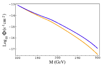
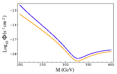
Figure 7: The flux of the monochromatic photons from the reaction $B_{H}B_{H}\rightarrow\gamma\gamma$ in the pair-annihilation bands (left panel) and the coannihilation region (right panel). On the left panel, the blue/upper and the orange/lower lines correspond to the high and low solutions in Eq. (11), respectively. On the right panel, the blue/upper line corresponds to $m_{h}=300$ GeV, the orange/lower line to $m_{h}=120$ GeV. The plots assume $\bar{J}(\Psi,\Delta\Omega)\Delta\Omega=1$; all fluxes scale linearly with this parameter.

The monochromatic photon fluxes (assuming $\bar{J}\Delta\Omega=1$) predicted by the LHT model in the parameter regions where the heavy photon accounts for all of the observed dark matter, are shown in Fig. 7. The left panel corresponds to the pair-annihilation bands, and the right panel to the coannihilation region. Searches for gamma rays from WIMP annihilation have to be able to distinguish them from the astrophysical background. In the case of the monochromatic photons, the signal is concentrated in a single bin (the energy uncertainty of the telescopes is about 10%, much larger than the intrinsic line width), and the background can be effectively measured in the neighbouring bins and subtracted. In the relevant energy range, the flux sensitivity for ground-based Atmospheric Cherenkov Telescopes (ACTs) such as VERITAS [40] and HESS [41] is estimated to be around $(1-5)\times 10^{-12}$ cm^-2sec^-1, whereas the sensitivity of the upcoming space-based telescope GLAST is limited by statistics at $10^{-10}$ cm^-2sec^-1, assuming that 10 events are required to claim discovery [42]. It is clear that the monochromatic flux predicted by the LHT model is beyond the reach of GLAST, but could be observed at the ACTs if the dark matter distribution in the halo exhibits a substantial spike or strong clumping, $\bar{J}\mathrel{\mathchoice{\lower 2.5pt\vbox{\halign{$\mathsurround 0pt\displaystyle\hfil#\hfil$\cr>\crcr\sim\crcr}}}{\lower 2.5pt\vbox{\halign{$\mathsurround 0pt\textstyle\hfil#\hfil$\cr>\crcr\sim\crcr}}}{\lower 2.5pt\vbox{\halign{$\mathsurround 0pt\scriptstyle\hfil#\hfil$\cr>\crcr\sim\crcr}}}{\lower 2.5pt\vbox{\halign{$\mathsurround 0pt\scriptscriptstyle\hfil#\hfil$\cr>\crcr\sim\crcr}}}}10^{5}$ at $\Delta\Omega\approx 10^{-3}$.

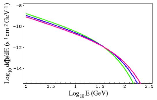
Figure 8: The fragmentation photon flux for $M=150,200,250$ GeV (green, blue and red lines, respectively), in the pair-annihilation bands. The plot assumes $\bar{J}(\Psi,\Delta\Omega)\Delta\Omega=1$; all fluxes scale linearly with this parameter.

Let us now consider the component of the photon flux due to hadronization and fragmentation of quarks produced in WIMP annihilation. As discussed in Section 3, the heavy photons predominantly annihilate into $W$ and $Z$ pairs; each of the vector bosons can in turn decay into a quark pair. The resulting photon spectra depend only on the initial energies of the $W$’s and $Z$’s, and not on the details of the WIMP annihilation process. The spectra have been studied using PYTHIA (in the MSSM context), and a simple analytic fit has been presented in Ref. [35]:

$$\frac{dN_{\gamma}}{dx}\approx\frac{0.73}{x^{1.5}}e^{-7.8x}.$$ (31)

where $x=E_{\gamma}/M$. This approximation is valid for both $W^{+}W^{-}$ and $ZZ$ final states. In the pair-annihilation bands, the differential flux is then given by

$$\frac{d\Phi}{dE}\,=\,\left(3.3\times 10^{-12}{\rm s}^{-1}{\rm cm}^{-2}{\rm GeV}^{-1}\right)\,x^{-1.5}e^{-7.8x}\,\left(\frac{100~{}{\rm GeV}}{M}\right)^{3}\bar{J}(\Psi,\Delta\Omega)\Delta\Omega,$$ (32)

where we used the relic density constraint, $a(W^{+}W^{-})+a(ZZ)\approx 0.8$ pb. The flux in the coannihilation region is much smaller.

The fluxes predicted by Eq. (32) for several values of $M$ are plotted in Fig. 8. The GLAST telescope is statistics-limited at energies above about 2 GeV, and would observe tens of events in this energy range for the heavy photon mass in the preferred range, assuming $\bar{J}(\Delta\Omega)\Delta\Omega=1$. (The flux scales linearly with this parameter combination.) One should keep in mind, however, that while the prospects for observing this signal are good, ruling out its interpretation in terms of conventional astrophysics could be challenging given the smooth, featureless nature of the fragmentation spectrum. Detailed studies of the angular distribution of these photons, in particular outside the galactic disk, will be needed.

The ACTs have a higher energy threshold, typically about 50 GeV, and suffer from an irreducible background from electron-induced showers, about $10^{-12}-10^{-10}$ cm^-2s^-1GeV^-1 in the relevant energy range ($50\ldots 200$ GeV) for $\Delta\Omega\sim 10^{-3}$. Using the extraploation of Ref. [35] to estimate the background, we find that the typical signal/background ratio expected at the ACTs, assuming $\Delta\Omega\sim 10^{-3}$ and $\bar{J}(\Delta\Omega)\Delta\Omega=1$, is only about $10^{-3}$. An observation of the fragmentation flux at the ACTs appears quite challenging, unless dark matter is strongly clustered at the galactic center or clumped.

The third and final component of the gamma-ray flux from WIMP annihilation is the final state radiation (FSR) photons. The FSR flux generally provides a robust signature of WIMP annihilation: it exists whenever the WIMPs have a sizable annihilation cross section into any charged states. The FSR photons have a continuous spectrum, in analogy to the quark fragmentation photons consdered above. In fact, at low energies, the fragmentation flux dominantes over the FSR component (unless WIMPs annihilate into purely leptonic states). At energies close to the WIMP mass, however, the fragmentation flux drops sharply, and the FSR component typically dominates [43]. This is particularly interesting because the FSR spectrum typically possesses a sharp edge feature, abruptly dropping to zero at the maximal photon energy allowed by kinematics. The edge feature could help the experiments to discern this flux on top of the (a priori highly uncertain) astrophysical background, and provide a measurement of the WIMP mass [43]. In the LHT model, the dominant charged two-body annihilation channel is $W^{+}W^{-}$, and correspondingly the reaction $B_{H}B_{H}\rightarrow W^{+}W^{-}\gamma$ provides the most important component of the FSR photon flux. The differential cross section for this process is given by

$$\frac{d\sigma}{dx}\left(B_{H}B_{H}\rightarrow W^{+}W^{-}\gamma\right)=\sigma\left(B_{H}B_{H}\rightarrow W^{+}W^{-}\right)\,{\cal F}(x;\mu_{w}),$$ (33)

where $x=2E_{\gamma}/\sqrt{s}\approx E_{\gamma}/M$, $\mu_{w}=(m_{W}/M)^{2}$ and

$${\cal F}(x;\mu) = \frac{\alpha}{\pi}\frac{1}{\sqrt{1-\mu}}\,\frac{1}{x}\,\times\Bigl{[}(2x-2+\mu)\log\frac{2(1-x)-\mu-2\sqrt{(1-x)(1-x-\mu)}}{\mu}$$ (34)

$$+2\left(\frac{8x^{2}}{4-4\mu+3\mu^{2}}-1\right)\sqrt{(1-x)(1-x-\mu)}\Bigr{]}\,,$$

for $0\leq x\leq 1-\mu$ and 0 for $1-\mu\leq x\leq 1$. In the limit of large heavy photon mass, $s\gg M_{W}^{2}$, this expression reduces to

$${\cal F}(x)=\frac{2\alpha}{\pi}\frac{1-x}{x}\,\Bigl{[}\log\frac{s(1-x)}{m_{W}^{2}}\,+\,2x^{2}-1+{\cal O}(\mu)\Bigr{]}.$$ (35)

The leading (logarithmically enhanced) term agrees with the result obtained in Ref. [43] using the Goldstone boson equivalence theorem. Note that the form of the photon emission factor ${\cal F}$, even in the large-$s$ limit, depends on the theory being considered and on the initial state. For example, the $\tilde{\chi}_{1}^{0}\tilde{\chi}_{1}^{0}\rightarrow W^{+}W^{-}\gamma$ cross section in the MSSM, computed in Ref. [44], has a different leading logarithm behavior; this is related to the fact that the $W$ bosons effectively become massless in this limit, inducing new infrared singularities. Thus, even though we chose to write the cross section (33) in a “factorized” form, there is no true factorization in the $WW\gamma$ final state, in contrast to the $f\bar{f}\gamma$ final states [43].

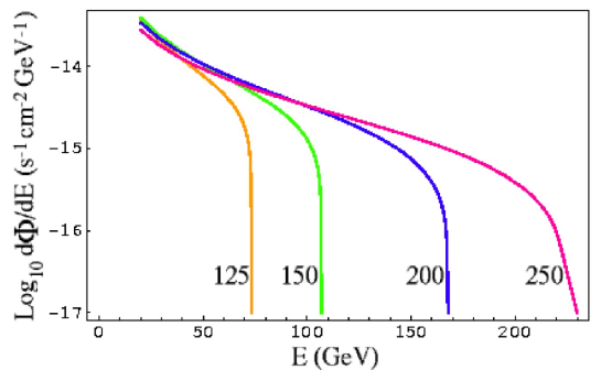
Figure 9: The FSR photon flux for $M=125,150,200,250$ GeV (left to right), in the pair-annihilation bands. (The fluxes for “high” and “low” solutions are essentially identical.) The plot assumes $\bar{J}(\Psi,\Delta\Omega)\Delta\Omega=1$; all fluxes scale linearly with this parameter.

The flux of the FSR photons is given by

$$\frac{d\Phi}{dE}\,=\,\left(5.6\times 10^{-12}{\rm s}^{-1}{\rm cm}^{-2}{\rm GeV}^{-1}\right)\,\left(\frac{a(W^{+}W^{-})}{1{\rm~{}pb}}\right)\,{\cal F}(x;\mu_{w})\,\left(\frac{100~{}{\rm GeV}}{M}\right)^{3}\bar{J}(\Psi,\Delta\Omega)\Delta\Omega,$$ (36)

where $a(W^{+}W^{-})$ is given in Eq. (LABEL:wz). Flux predictions for several representative values of $M$ are shown in Fig. 9. In each case, the flux drops abruptly at the maximal photon energy,

$$E^{\gamma}_{\rm max}\,=\,\frac{M^{2}-m_{W}^{2}}{M}.$$ (37)

If this edge feature is observed, it would provide a robust signature of heavy photon annihilation, as well as a measurement of its mass. Note that the FSR and fragmentation components of the flux are comparable near the edge, so that the fractional drop in the “signal” flux at the edge is significant. Just as for the monochromatic and fragmentation photons, the sensitivity to the FSR flux at ACTs is limited by the background from electron-induced showers. Assuming a 10% uncertainty on the total flux measurement, the drop in the total flux associated with the edge feature of the FSR spectrum can be observed if $\bar{J}\mathrel{\mathchoice{\lower 2.5pt\vbox{\halign{$\mathsurround 0pt\displaystyle\hfil#\hfil$\cr>\crcr\sim\crcr}}}{\lower 2.5pt\vbox{\halign{$\mathsurround 0pt\textstyle\hfil#\hfil$\cr>\crcr\sim\crcr}}}{\lower 2.5pt\vbox{\halign{$\mathsurround 0pt\scriptstyle\hfil#\hfil$\cr>\crcr\sim\crcr}}}{\lower 2.5pt\vbox{\halign{$\mathsurround 0pt\scriptscriptstyle\hfil#\hfil$\cr>\crcr\sim\crcr}}}}10^{5}-10^{6}$. The sensitivity at GLAST is limited by statistics, and an observation of the FSR edge requires even higher values of $\bar{J}$.

To summarize, we found that the best prospects for a discovery of anomalous gamma rays due to heavy photon annihilation in the Milky Way are offered by the GLAST telescope, which should be able to observe tens of fragmentation photons in the multi-GeV energy range. The fluxes of monochromatic and FSR photons, whose spectra would provide clear signatures for galactic WIMP annihilation (a bump and an edge, respectively), are significantly smaller. The prospects for their detection depend on the assumed halo profile; an observation by the ACTs such as VERITAS and HESS is possible if the dark matter density has a sharp peak at the galactic center or is strongly clumped, $\bar{J}\mathrel{\mathchoice{\lower 2.5pt\vbox{\halign{$\mathsurround 0pt\displaystyle\hfil#\hfil$\cr>\crcr\sim\crcr}}}{\lower 2.5pt\vbox{\halign{$\mathsurround 0pt\textstyle\hfil#\hfil$\cr>\crcr\sim\crcr}}}{\lower 2.5pt\vbox{\halign{$\mathsurround 0pt\scriptstyle\hfil#\hfil$\cr>\crcr\sim\crcr}}}{\lower 2.5pt\vbox{\halign{$\mathsurround 0pt\scriptscriptstyle\hfil#\hfil$\cr>\crcr\sim\crcr}}}}10^{5}-10^{6}$.

6 Conclusions

Little Higgs models provide an interesting alternative scenario for physics at the TeV scale, with a simple and attractive mechanism of radiative electroweak symmetry breaking. Many realistic models implementing the Little Higgs mechanism have been proposed; however, generically these models are ruled out by precision electroweak data, unless the scale $f$ is in a few-TeV range which reintroduces fine-tuning. Little Higgs models with T parity avoid this difficulty. In this paper, we focused on the Littlest Higgs model with T parity (LHT), one of the simplest models in this class. T parity makes the lightest of the T-odd particles, the LTP, stable, enabling it to have a substantial abundance in today’s universe in spite of its weak-scale mass. In the LHT model, the LTP is typically the heavy photon $B_{H}$, which can play the role of WIMP dark matter. We have computed the relic abundance of this particle, including coannihilation effects, and mapped out the regions of the parameter space where it has the correct relic abundance to account for all, or a substantial part, of the observed dark matter. These regions can be divided into the pair-annihilation bands, where the abundance is set by the $B_{H}$ pair annihilation via $s$-channel Higgs resonance, and the coannihilation tail, where coannihilations of $B_{H}$ with T-odd quarks $\tilde{Q}$ and leptons $\tilde{L}$ play the dominant role.

In the second part of the paper, we evaluated the prospects for observing the heavy photon dark matter of the LHT model using direct and indirect detection techniques. Direct detection is quite difficult, due to the fact that the heavy photon predominantly couples to the Standard Model states via the Higgs boson whose interactions with nucleons are weak. The elastic cross section of the $B_{H}$ scattering on a nucleus in the region of parameter space consistent with the relic density constraint was found to be several orders of magnitude below the current sensitivity of direct detection searches such as CDMS. For indirect detection, we concentrated on the anomalous high-energy gamma ray signature. The predicted gamma ray flux depends sensitively on the distribution of dark matter in the halo. The best discovery prospect is offered by the GLAST telescope, which can observe the photons arising from the fragmentation of the $W/Z$ bosons produced in the heavy photon annihilation. If dark matter distribution in the halo is favorable (in particular if it ehxibits a sharp spike near the galactic center, or is highly clumpy on short scales), ground-based telescopes such as VERITAS and HESS may also be able to observe a gamma ray signal. In this case, it might also be possible to observe the monochromatic and the FSR components of the photon flux, whose spectra exhibit well-defined features (a line and an edge, respectively) and would provide a smoking-gun evidence for the WIMP-related nature of the signal.

Acknowledgments — We are grateful to Jay Hubisz and Patrick Meade for useful discussions. MP, AN and AS are supported by the NSF grant PHY-0355005.

MP is grateful to Prateek Agrawal and Can Kilic for pointing out a typo in Eq. (7) in the original version of the paper. None of the results beyond this formula were affected.

References

- [1] For a recent review and a collection of references, see G. Bertone, D. Hooper and J. Silk, Phys. Rept. 405, 279 (2005) [arXiv:hep-ph/0404175].
- [2] N. Arkani-Hamed, A. G. Cohen, E. Katz and A. E. Nelson, JHEP 0207, 034 (2002) [arXiv:hep-ph/0206021].
- [3] M. Schmaltz and D. Tucker-Smith, arXiv:hep-ph/0502182
- [4] M. Perelstein, arXiv:hep-ph/0512128.
- [5] G. Burdman, M. Perelstein and A. Pierce, Phys. Rev. Lett. 90, 241802 (2003) [Erratum-ibid. 92, 049903 (2004)] [arXiv:hep-ph/0212228]; T. Han, H. E. Logan, B. McElrath and L. T. Wang, Phys. Rev. D 67, 095004 (2003) [arXiv:hep-ph/0301040]; M. Perelstein, M. E. Peskin and A. Pierce, Phys. Rev. D 69, 075002 (2004) [arXiv:hep-ph/0310039].
- [6] C. Csaki, J. Hubisz, G. D. Kribs, P. Meade and J. Terning, Phys. Rev. D 67, 115002 (2003) [arXiv:hep-ph/0211124]; J. L. Hewett, F. J. Petriello and T. G. Rizzo, JHEP 0310, 062 (2003) [arXiv:hep-ph/0211218].
- [7] H. C. Cheng and I. Low, JHEP 0309, 051 (2003) [arXiv:hep-ph/0308199]; JHEP 0408, 061 (2004) [arXiv:hep-ph/0405243].
- [8] I. Low, JHEP 0410, 067 (2004) [arXiv:hep-ph/0409025].
- [9] J. Hubisz, P. Meade, A. Noble and M. Perelstein, JHEP 0601, 135 (2006) [arXiv:hep-ph/0506042].
- [10] D. E. Kaplan and M. Schmaltz, JHEP 0310, 039 (2003) [arXiv:hep-ph/0302049]; M. Schmaltz, JHEP 0408, 056 (2004) [arXiv:hep-ph/0407143].
- [11] A. Martin, arXiv:hep-ph/0602206.
- [12] A. Birkedal-Hansen and J. G. Wacker, Phys. Rev. D 69, 065022 (2004) [arXiv:hep-ph/0306161].
- [13] J. Hubisz and P. Meade, arXiv:hep-ph/0411264, v3. See also Phys. Rev. D 71, 035016 (2005); note however that the dark matter relic density plot has not been updated in the journal version.
- [14] J. Hubisz, S. J. Lee and G. Paz, arXiv:hep-ph/0512169.
- [15] H. C. Cheng, I. Low and L. T. Wang, arXiv:hep-ph/0510225.
- [16] A. Birkedal, K. Matchev and M. Perelstein, Phys. Rev. D 70, 077701 (2004) [arXiv:hep-ph/0403004].
- [17] G. Servant and T. M. P. Tait, Nucl. Phys. B 650, 391 (2003) [arXiv:hep-ph/0206071].
- [18] H. C. Cheng, J. L. Feng and K. T. Matchev, Phys. Rev. Lett. 89, 211301 (2002) [arXiv:hep-ph/0207125].
- [19] D. N. Spergel et al. [WMAP Collaboration], Astrophys. J. Suppl. 148, 175 (2003) [arXiv:astro-ph/0302209].
- [20] A. Pukhov, arXiv:hep-ph/0412191.
- [21] G. Belanger, F. Boudjema, A. Pukhov and A. Semenov, arXiv:hep-ph/0405253.
- [22] B. C. Allanach et al., arXiv:hep-ph/0602198, pp. 146–149.
- [23] R. J. Scherrer and M. S. Turner, Phys. Rev. D 33, 1585 (1986) [Erratum-ibid. D 34, 3263 (1986)].
- [24] L. B. Okun, Leptons and Quarks (1982), pp. 228-231.
- [25] G. K. Mallot, in Proc. of the 19th Intl. Symp. on Photon and Lepton Interactions at High Energy LP99 ed. J.A. Jaros and M.E. Peskin, Int. J. Mod. Phys. A 15S1, 521 (2000) [eConf C990809, 521 (2000)] [arXiv:hep-ex/9912040].
- [26] D. S. Akerib et al. [CDMS Collaboration], Phys. Rev. Lett. 96, 011302 (2006) [arXiv:astro-ph/0509259].
- [27] SuperCDMS (Projected) Phase C [from the Dark Matter Plotter web site, http://dmtools.berkeley.edu/limitplots/].
- [28] G. J. Alner et al. [UK Dark Matter Collaboration], Phys. Lett. B 616, 17 (2005) [arXiv:hep-ex/0504031].
- [29] N. J. C. Spooner et al., Phys. Lett. B 473, 330 (2000).
- [30] M. Asano, S. Matsumoto, N. Okada and Y. Okada, arXiv:hep-ph/0602157.
- [31] L. Bergstrom and P. Ullio, Nucl. Phys. B 504, 27 (1997) [arXiv:hep-ph/9706232]; Z. Bern, P. Gondolo and M. Perelstein, Phys. Lett. B 411, 86 (1997) [arXiv:hep-ph/9706538].
- [32] M. A. Shifman, A. I. Vainshtein, M. B. Voloshin and V. I. Zakharov, Sov. J. Nucl. Phys. 30, 711 (1979) [Yad. Fiz. 30, 1368 (1979)].
- [33] J. F. Gunion, H. E. Haber, G. L. Kane and S. Dawson, The Higgs Hunter’s Guide, Perseus, Cambridge, MA, 1990; see also arXiv:hep-ph/9302272.
- [34] C. R. Chen, K. Tobe and C. P. Yuan, arXiv:hep-ph/0602211.
- [35] L. Bergstrom, P. Ullio and J. H. Buckley, Astropart. Phys. 9, 137 (1998) [arXiv:astro-ph/9712318].
- [36] K. Kosack et al. [The VERITAS Collaboration], Astrophys. J. 608, L97 (2004) [arXiv:astro-ph/0403422]; K. Tsuchiya et al. [CANGAROO-II Collaboration], Astrophys. J. 606, L115 (2004) [arXiv:astro-ph/0403592]; F. Aharonian et al. [The HESS Collaboration], Astron. Astrophys. 425, L13 (2004) [arXiv:astro-ph/0408145].
- [37] J. F. Navarro, C. S. Frenk and S. D. M. White, Astrophys. J. 490, 493 (1997).
- [38] B. Moore, F. Governato, T. Quinn, J. Stadel and G. Lake, Astrophys. J. 499, L5 (1998) [arXiv:astro-ph/9709051]; B. Moore, T. Quinn, F. Governato, J. Stadel and G. Lake, Mon. Not. Roy. Astron. Soc. 310, 1147 (1999) [arXiv:astro-ph/9903164].
- [39] G. R. Blumenthal, S. M. Faber, R. Flores and J. R. Primack, Astrophys. J. 301, 27 (1986); F. Prada, A. Klypin, J. Flix, M. Martinez and E. Simonneau, arXiv:astro-ph/0401512; O. Y. Gnedin, A. V. Kravtsov, A. A. Klypin and D. Nagai, Astrophys. J. 616, 16 (2004) [arXiv:astro-ph/0406247].
- [40] T. C. Weekes et al., Astropart. Phys. 17, 221 (2002) [arXiv:astro-ph/0108478].
- [41] J. A. Hinton [The HESS Collaboration], New Astron. Rev. 48, 331 (2004) [arXiv:astro-ph/0403052].
- [42] A. Morselli, A. Lionetto, A. Cesarini, F. Fucito and P. Ullio [GLAST Collaboration], Nucl. Phys. Proc. Suppl. 113, 213 (2002) [arXiv:astro-ph/0211327].
- [43] A. Birkedal, K. T. Matchev, M. Perelstein and A. Spray, arXiv:hep-ph/0507194.
- [44] L. Bergstrom, T. Bringmann, M. Eriksson and M. Gustafsson, Phys. Rev. Lett. 95, 241301 (2005) [arXiv:hep-ph/0507229].