THE FUNDAMENTAL SYMMETRIES IN THE NEUTRAL KAON SYSTEM
– a pedagogical choice –

Abstract

During the recent years experiments with neutral kaons have yielded remarkably sensitive results which are pertinent to such fundamental phenomena as $\mathrm{\cal CPT}$ invariance (protecting causality), time-reversal invariance violation, coherence of wave functions, and entanglement of kaons in pair states. We describe the phenomenological developments and the theoretical conclusions drawn from the experimental material. An outlook to future experimentation is indicated.

March 1, 2006

1 Introduction

Symmetries, here, designate certain properties of theoretically formulated laws of physics. For the experimental investigation of these laws, symmetries are of great utility. They establish simple and reliable relations between the abstract law and specific, in practice, observable quantities. In this article, we shall encounter symmetry properties of the experimental data, that directly reflect symmetry properties of the physical law. Examples are given in Table 1.

Fundamental symmetries shall be those ones which concern space and time in our world, or in the unavoidable antimatter world. Since many laws govern evolutions in space and time, fundamental symmetries have a wide range of applications and are valid under very general provisions, most often conveniently independent on unknown details.
In the search for the formal properties of a law, experimentally observed symmetries are most valuable guide lines.

For a causal description of Nature, where the future is connected to the past, it is necessary, that the law of time evolution is endowed with an invariance, with respect to such a symmetry operation, that contains, at least, a reversal of the arrow of time. Res Jost [1], pioneer of the $\mathrm{\cal CPT}$ theorem [2, 5, 3, 4, 6], writes ’… : eine kausale Beschreibung ist nur möglich, wenn man den Naturgesetzen eine Symmetrie zugesteht, welche den Zeitpfeil umkehrt’.
The only suitable symmetry for this purpose, not found violated (yet), is a combination: the symmetry with respect to the $\mathrm{\cal CPT}$ transformation, where time and space coordinates are reflected at their origins ($\mathrm{\cal T}$ and $\mathrm{\cal P}$), and particles become antiparticles ($\mathrm{\cal C}$). (We remember that each and every one alone of the symmetries with respect to  $\mathrm{\cal C}$, $\mathrm{\cal P}$ or $\mathrm{\cal T}$ are not respected by weak interactions).

The property of  $\mathrm{\cal CPT}$ symmetry entails the existence of antimatter, and the equality of the masses and the decay widths of a particle and of its antiparticle.

We shall describe the cleverness, the favorable natural circumstances, and the experimental ingenuity, that allowed one to achieve the extraordinary insight, that the masses and the decay widths of  $\mathrm{K^{0}}$ and $\mathrm{\overline{K}}{}^{0}$ are really equal, within about one in $10^{18}$ (!).

$\mathrm{\cal CPT}$ symmetry is not implied by quantum mechanics (QM). If wanted, it has to be implemented as an extra property of the Hamiltonian in the Schrödinger equation. This allows one to also formulate hypothetical  $\mathrm{\cal CPT}$ symmetry violating processes within QM, and to devise appropriate experimental searches.
We shall describe experimental results that could have contradicted $\mathrm{\cal CPT}$ invariance, but did not.

Two-state systems, treated by quantum mechanics, introduce an additional hierarchy among the symmetry violations: the detection of a violation of the  $\mathrm{\cal CPT}$ or (and)  of the $\mathrm{\cal T}$ symmetry implies a  $\mathrm{\cal CP}$ symmetry violation. This is exemplified by the third column of Table 1. Furthermore, they exhibit the difficulty, that a  $\mathrm{\cal T}$ symmetry violation can, in these systems, only be defined, if a decay process exists, which is, by its nature, inherently  $\mathrm{\cal T}$ asymmetric. This has brought on the question, whether the observed effect of  $\mathrm{\cal T}$ symmetry violation in the  $\mathrm{K^{0}}$ $\mathrm{\overline{K}}{}^{0}$ system is a genuine property of the weak interaction, or whether it is just an artifact of the decaying two-state system.
We shall describe the way out of this maze. It consists of formulating  $\mathrm{\cal T}$ symmetry not on the level of the two-state system, but in the complete environment, which comprises all the states involved, including the decay products, and where the Hamiltonian is (thus) hermitian; and then to show that a  $\mathrm{\cal T}$ symmetric Hamiltonian would not be able to reproduce the experimental data.

There is only one place in particle physics, where a  $\mathrm{\cal T}$ asymmetry has been detected [7, 8]:
the  $\mathrm{\overline{K}}{}^{0}$ develops faster towards a $\mathrm{K^{0}}$ than does a  $\mathrm{K^{0}}$ towards a $\mathrm{\overline{K}}{}^{0}$.

The interpretation of non-vanishing ’$\mathrm{\cal T}$- odd’ quantities as signals for  $\mathrm{\cal T}$ asymmetry, is plagued by  $\mathrm{\cal T}$ symmetric effects, such as final state interactions, which also are able to produce non-vanishing $\mathrm{\cal T}$- odd results. We discuss an experiment which has achieved to yield a sizable $\mathrm{\cal T}$- odd correlation under a  $\mathrm{\cal T}$ symmetric law, even in the absence of final state interactions. (We know of no other case in particle physics, where this happens).

Particles with two states occur at various, independent places in physics, where they exhibit widely different phenomena. However, when a quantum mechanical description based on two-component wave functions is appropriate, then these phenomena display formally identical patterns, with common properties, such as the number of free parameters, or as the fact that there is only one basic observable at choice, whose expectation value can be determined in a single measurement with an unambiguous result.

The insight into the nature of these common properties is most elegantly achieved with the ’Pauli matrix toolbox’, which we freely use in this article. (The Appendix gives a description at an introductory level).

Could we test quantum mechanics ? Could we find out whether  $\mathrm{\cal CPT}$ symmetry could appear violated, not because of a  $\mathrm{\cal CPT}$ asymmetry of the Hamiltonian, but because the way, we apply the common rules of QM, is inadequate ?
We shall describe how it has been possible to conclude, that a hypothetical, hidden QM violating energy would have to be tinier than about $10^{-21}$ $\mathrm{GeV}$, in order to have escaped the existing experiments with neutral kaons[9]. (The extension of the Pauli matrix toolbox to density matrices will be introduced).

One of the most sensational predictions of QM is teleportation, which appears between two distant particles in an entangled state. As experimentation at  $\phi$ factories with entangled neutral kaons is growing, we shall give the basic formal toolbox for two-particle systems, where each particle is a decaying two-state system, and where QM rules are not necessarily respected.

The main body of this article explains, how the unique properties of the neutral kaons have been used to investigate the properties of the fundamental symmetries. To do justice to those students, who want to worry about the weak points in the thoughts, we present the most important doubts about side effects, which could have endangered the validity of the conclusions.

A neutral kaon oscillates forth and back between itself and its antiparticle, because the physical quantity, strangeness, which distinguishes antikaons from kaons, is not conserved by the interaction which governs the time evolution [10, 11]. A neutral kaon is by itself a two-state system.
The oscillation here can be viewed in analogy to the spin precession of a nucleon in a magnetic field, but where the rôle of the field is carried out by the inherent weak interaction of the kaon. The spin manipulation in NMR experiments by radio wave pulses corresponds to the application of  coherent regeneration, a phenomenon which occurs, when neutral kaons traverse matter.

The experimentation with neutral kaons provides the researcher with an impressing scene. The interference pattern of matter waves becomes visible in macroscopic dimensions !

Think of two highly stable damped oscillators with a relative frequency difference of  $\approx 7\times 10^{-15}$. The corresponding beat frequency of  $\approx 5.3\times 10^{9}\ \mathrm{s}^{-1}$, and the scale of the resulting spatial interference pattern of  $\approx 0.36$ m are ideally adapted to the technical capabilities of detectors in high-energy physics.

The extreme sensitivity of the neutral kaon system comes from the tiny mass difference $\Delta m$ of the exponentially decaying states. Some fraction of the size of $\Delta m\approx 3.5\times 10^{-15}\mathrm{GeV}$, depending on the measurement’s precision, determines the level for effects, which may be present inside of the equation of motion, to which the measurements are sensitive: $10^{-18}$ to $10^{-21}\mathrm{GeV}$.

The history of the unveilings of the characteristics of the neutral kaons is a sparkling succession of brilliant ideas and achievements, theoretical and experimental [12, 13, 14, 15, 16, 17, 18, 19].
We have reasons to assume that neutral kaons will enable one to make more basic discoveries. Some of the kaons’ properties (e. g. entanglement) have up to now only scarecely been exploited.

2 The neutral-kaon system

2.1 Time evolution

The time evolution of a neutral kaon and of its decay products may be represented by the state vector

$$\ket{\psi}=\psi_{\mathrm{K^{0}}}(t)\ket{\mathrm{K^{0}}}+\psi_{\mathrm{\overline{K}}{}^{0}}(t)\ket{\mathrm{\overline{K}}{}^{0}}+\sum_{m}c_{m}(t)\ket{m}$$ (1)

which satisfies the Schrödinger equation

$$\mathrm{i}\frac{\mathrm{d}\ket{\psi}}{\mathrm{d}t}=\mathrm{{\cal H}}\ket{\psi}.$$ (2)

In the Hamiltonian, $\mathrm{{\cal H}}=\mathrm{{\cal H}}_{0}+\mathrm{{\cal H}_{wk}}$, $\mathrm{{\cal H}}_{0}$ governs the strong and electromagnetic interactions. It is invariant with respect to the transformations $\mathrm{\cal C}$, $\mathrm{\cal P}$, $\mathrm{\cal T}$, and it conserves the strangeness $S$. The states $\ket{\mathrm{K^{0}}}$ and $\ket{\mathrm{\overline{K}}{}^{0}}$ are common stationary eigenstates of $\mathrm{{\cal H}}_{0}$ and $S$, with the mass $m_{0}$ and with opposite strangeness: $\mathrm{{\cal H}}_{0}\ket{\mathrm{K^{0}}}=m_{0}\ket{\mathrm{K^{0}}}$, $\mathrm{{\cal H}}_{0}\ket{\mathrm{\overline{K}}{}^{0}}=m_{0}\ket{\mathrm{\overline{K}}{}^{0}}$, $S\ket{\mathrm{K^{0}}}=\ket{\mathrm{K^{0}}}$, $S\ket{\mathrm{\overline{K}}{}^{0}}=-\ket{\mathrm{\overline{K}}{}^{0}}$. The states $\ket{m}$ are continuum eigenstates of $\mathrm{{\cal H}}_{0}$ and represent the decay products. They are absent at the instant of production $(t=0)$ of the neutral kaon. The initial condition is thus

$$\ket{\psi_{0}}=\psi_{\mathrm{K^{0}}}(0)\ket{\mathrm{K^{0}}}+\psi_{\mathrm{\overline{K}}{}^{0}}(0)\ket{\mathrm{\overline{K}}{}^{0}}\ .$$ (3)

$\mathrm{{\cal H}_{wk}}$  governs the weak interactions. Since these do not conserve strangeness, a neutral kaon will, in general, change its strangeness as time evolves.

Equation (2) may be solved for the unknown functions $\psi_{\mathrm{K^{0}}}(t)$ and $\psi_{\mathrm{\overline{K}}{}^{0}}(t)$ , by using a perturbation approximation [20] which yields [21, 22]

$$\psi=\mathrm{e}^{-\mathrm{i}\Lambda t}\psi_{0}\ .$$ (4)

$\psi$ is the column vector with components $\psi_{\mathrm{K^{0}}}(t)$ and $\psi_{\mathrm{\overline{K}}{}^{0}}(t)$, $\psi_{0}$ equals $\psi$ at $t=0$, and $\Lambda$ is the time-independent $2\times 2$ matrix $\left(\mathrm{\Lambda_{\alpha\alpha^{\prime}}}\right)$, whose components refer to the two-dimensional basis $\ket{\mathrm{K^{0}}},\ket{\mathrm{\overline{K}}{}^{0}}$ and may be written as  $\mathrm{\Lambda_{\alpha\alpha^{\prime}}}$ =  $\bra{\alpha}\Lambda\ket{\alpha^{\prime}}$ with $\alpha,\alpha^{\prime}=\mathrm{K^{0}},\mathrm{\overline{K}}{}^{0}$.

Since the kaons decay, we have

$$0>\frac{\mathrm{d}|\psi|^{2}}{\mathrm{d}t}=-\mathrm{i}\psi^{\dagger}\left(\Lambda-\Lambda^{\dagger}\right)\psi\,.$$ (5)

$\Lambda$ is thus not hermitian, $\mathrm{e}^{-\mathrm{i}\Lambda t}$ is not unitary, in general.

This motivates the definition of $\mathrm{M}$ and $\mathrm{\Gamma}$ as

$$\Lambda = \mathrm{M}-\frac{\mathrm{i}}{2}\mathrm{\Gamma}\;,$$ (6a)

$$\mathrm{M} = \mathrm{M}^{\dagger},\quad\mathrm{\Gamma}=\mathrm{\Gamma}^{\dagger}\;.$$ (6b)

We find

$$0>\frac{\mathrm{d}|\psi|^{2}}{\mathrm{d}t}=-\psi^{\dagger}\mathrm{\Gamma}\psi\;.$$ (7)

This expresses that $\mathrm{\Gamma}$ has to be a positive matrix.

The perturbation approximation also establishes the relation from $\mathrm{{\cal H}_{wk}}$ to $\Lambda$ (including second order in $\mathrm{{\cal H}_{wk}}$) by

$$\mathrm{M}_{\alpha\alpha^{\prime}} =m_{0}\delta_{\alpha\alpha^{\prime}}+\langle\alpha|\mathrm{{\cal H}_{wk}}|\alpha^{\prime}\rangle+\mathrm{\cal P}\sum_{\beta}\left(\frac{\langle\alpha|\mathrm{{\cal H}_{wk}}|\beta\rangle\langle\beta|\mathrm{{\cal H}_{wk}}|\alpha^{\prime}\rangle}{m_{0}-E_{\beta}}\right)\;,$$ (8a)

$$\mathrm{\Gamma}_{\alpha\alpha^{\prime}} =2\pi\sum_{\beta}\langle\alpha|\mathrm{{\cal H}_{wk}}|\beta\rangle\langle\beta|\mathrm{{\cal H}_{wk}}|\alpha^{\prime}\rangle\delta(m_{0}-E_{\beta})\;,$$ (8b)

$$(\alpha,\alpha^{\prime} =\mathrm{K^{0}},\mathrm{\overline{K}}{}^{0})\,.$$

Equations (8a, 8b) enable one now to state directly the symmetry properties of $\mathrm{{\cal H}_{wk}}$  in terms of experimentally observable relations among the elements of $\Lambda$, see Table 1 and Ref. [23] . We remark that $\mathrm{\cal CPT}$ invariance imposes no restrictions on the off-diagonal elements, and that $\mathrm{\cal T}$ invariance imposes no restrictions on the diagonal elements of $\Lambda$ .  $\mathrm{\cal CP}$ invariance is violated, whenever one, at least, of these invariances is violated.

Table 1: The symmetry properties of $\mathrm{{\cal H}_{wk}}$ induce symmetries in observable quantities.

The last column indicates asymmetries of quantities which have been measured

by the CPLEAR experiment at CERN. More explanations are given in the text.

If $\mathrm{{\cal H}_{wk}}$ has the property	called	then	or
$\mathrm{\cal T}^{-1}\ \mathrm{{\cal H}_{wk}}\ \ \mathrm{\cal T}=\mathrm{{\cal H}_{wk}}$	$\mathrm{\cal T}$ invariance	$|\mathrm{\Lambda_{\mathrm{K^{0}}\mathrm{\overline{K}}{}^{0}}}|=|\mathrm{\Lambda_{\mathrm{\overline{K}}{}^{0}\mathrm{K^{0}}}}|$	$A_{\mathrm{T}}=0$
$(\mathrm{\cal CPT})^{-1}\ \mathrm{{\cal H}_{wk}}\ \ (\mathrm{\cal CPT})=\mathrm{{\cal H}_{wk}}$	$\mathrm{\cal CPT}$ invariance	$\ \ \mathrm{\Lambda_{\mathrm{K^{0}}\mathrm{K^{0}}}}=\ \mathrm{\Lambda_{\mathrm{\overline{K}}{}^{0}\mathrm{\overline{K}}{}^{0}}}$	$A_{\mathrm{CPT}}=0$
$(\mathrm{\cal CP})^{-1}\ \mathrm{{\cal H}_{wk}}\ \ (\mathrm{\cal CP})=\mathrm{{\cal H}_{wk}}$	$\mathrm{\cal CP}$  invariance	$\ \ \mathrm{\Lambda_{\mathrm{K^{0}}\mathrm{K^{0}}}}=\ \mathrm{\Lambda_{\mathrm{\overline{K}}{}^{0}\mathrm{\overline{K}}{}^{0}}}$  and
		$|\mathrm{\Lambda_{\mathrm{K^{0}}\mathrm{\overline{K}}{}^{0}}}|=|\mathrm{\Lambda_{\mathrm{\overline{K}}{}^{0}\mathrm{K^{0}}}}|$	$A_{\mathrm{CP}}=0$

The definitions of $\ket{\mathrm{K^{0}}}$ and $\ket{\mathrm{\overline{K}}{}^{0}}$ leave a real phase $\vartheta$ undetermined:

Since $S^{-1}\ \mathrm{{\cal H}}_{0}\ S=\ \mathrm{{\cal H}}_{0}$, the states

$$\ket{\mathrm{K^{0}}^{\prime}} = \mathrm{e}^{\mathrm{i}\vartheta S}\ket{\mathrm{K^{0}}}\ =\ \mathrm{e}^{\mathrm{i}\vartheta}\ \ \ket{\mathrm{K^{0}}}\ ,$$ (9a)

$$\ket{{\mathrm{\overline{K}}{}^{0}}^{{}^{\prime}}} = \mathrm{e}^{\mathrm{i}\vartheta S}\ket{\mathrm{\overline{K}}{}^{0}}\ =\ \mathrm{e}^{-\mathrm{i}\vartheta}\ket{\mathrm{\overline{K}}{}^{0}}\ .$$ (9b)

fulfil the definitions of $\ket{\mathrm{K^{0}}}$ and $\ket{\mathrm{\overline{K}}{}^{0}}$ as well, and constitute thus an equivalent basis which is related to the original basis by a unitary transformation. As the observables are always invariant with respect to unitary base transformations, the parameter $\vartheta$ cannot be measured, and remains undetermined. This has the effect that expressions which depend on $\vartheta$ are not suited to represent experimental results, unless $\vartheta$ has beforehand been fixed to a definite value by convention. Although such a convention may simplify sometimes the arithmetic, it risks to obscure the insight as to whether a certain result is genuine or whether it is just an artifact of the convention.
As an example we consider the elements of $\Lambda$, $\mathrm{\Lambda_{\alpha\alpha^{\prime}}}$ =  $\bra{\alpha}\Lambda\ket{\alpha^{\prime}}$ which refer to the basis $\alpha,\alpha^{\prime}=\mathrm{K^{0}},\mathrm{\overline{K}}{}^{0}$. With respect to the basis $\mathrm{e}^{\mathrm{i}\vartheta}\mathrm{K^{0}}$, $\mathrm{e}^{-\mathrm{i}\vartheta}\mathrm{\overline{K}}{}^{0}$ we obtain the same diagonal elements, whereas the off-diagonal elements change into

$$\mathrm{\Lambda_{\mathrm{K^{0}}\mathrm{\overline{K}}{}^{0}}} \longmapsto \Lambda^{\prime}_{\mathrm{K^{0}}\mathrm{\overline{K}}{}^{0}}\ =\ \mathrm{e}^{-2\mathrm{i}\vartheta}\ \ \mathrm{\Lambda_{\mathrm{K^{0}}\mathrm{\overline{K}}{}^{0}}}\ ,$$ (10a)

$$\mathrm{\Lambda_{\mathrm{\overline{K}}{}^{0}\mathrm{K^{0}}}} \longmapsto \Lambda^{\prime}_{\mathrm{\overline{K}}{}^{0}\mathrm{K^{0}}}\ =\ \mathrm{e}^{2\mathrm{i}\vartheta}\ \ \ \ \mathrm{\Lambda_{\mathrm{\overline{K}}{}^{0}\mathrm{K^{0}}}}\ ,$$ (10b)

and are thus convention dependent. However, their product, their absolute values, the trace tr{$\Lambda$}, its determinant, and its eigenvalues (not so its eigenvectors), but also the partition into $M$ and $\mathrm{\Gamma}$, are convention independent  [24]. (We will introduce a phase convention later in view of comparing experimental results).

The definition of the operations $\mathrm{\cal CP}$ and $\mathrm{\cal CPT}$ allows one to define two additional phase angles. We select them such that  $\cal{O}\mathrm{K^{0}}=$ $\mathrm{\overline{K}}{}^{0}$ and  $\cal{O}$$\mathrm{\overline{K}}{}^{0}$= $\mathrm{K^{0}}$, where $\cal{O}$ stands for $\mathrm{\cal CP}$ or $\mathrm{\cal CPT}$. See e. g. [25].

In order to describe the time evolution of a neutral kaon, the matrix exponential $\mathrm{e}^{-\mathrm{i}\Lambda t}$ has to be calculated.
If the exponent matrix has $two$ dimensions, a generalized Euler formula gives a straightforward answer.
Be $\Lambda$ represented as a superposition of Pauli matrices

$$\Lambda=\Lambda^{\mu}\sigma^{\mu}$$ (11)

with $\sigma^{0}$ =  unit matrix, $\sigma^{k}$ =  Pauli matrices, $\Lambda^{\mu}$ complex. (Summation over multiple indices: Greek 0 to 3, Roman 1 to 3).

Then

$$\mathrm{e}^{-\mathrm{i}\Lambda t}=\mathrm{e}^{-\mathrm{i}\Lambda^{\mu}\sigma^{\mu}t}=\mathrm{e}^{-\mathrm{i}\Lambda^{0}t}(\sigma^{0}\cos(\Omega t)-\mathrm{i}\Lambda^{m}\sigma^{m}t\sin(\Omega t)/(\Omega t)),$$ (12)

where  $\Omega^{2}=\ \Lambda^{m}\Lambda^{m}$. Noting that $\Lambda^{\mu}=\frac{1}{2}$tr$\{\sigma^{\mu}\Lambda\}$, we see that Eq. (12) expresses $\mathrm{e}^{-\mathrm{i}\Lambda t}$ entirely in terms of the elements of $\Lambda$. Since the (complex) eigenvalues $\mathrm{\lambda_{L}}$, $\mathrm{\lambda_{S}}$ of $\Lambda$ turn out to be observable (and are thus doubtless phase transformation invariant) we introduce them into (12).
They fulfil $\mathrm{\lambda_{L}}\mathrm{\lambda_{S}}=\mathrm{det}(\Lambda)=\Lambda^{0}\Lambda^{0}-\Lambda^{m}\Lambda^{m}$, and $\mathrm{\lambda_{L}}+\mathrm{\lambda_{S}}=\$tr$\{\Lambda\}=2\Lambda^{0}$, and thus, with $\mathrm{\Delta\lambda}\equiv\mathrm{\lambda_{L}}-\mathrm{\lambda_{S}}$,

$$\Omega=\mathrm{\Delta\lambda}/2\;.$$ (13)

We note here (with relief) that the calculation of the general time evolution, expressed in Eq. (4), does not need the knowledge of the $eigenstates$ of $\Lambda$, whose physical interpretation needs special attention  [26, 27].
The following corollary will be of interest:
The off-diagonal elements of a $2\times 2$ exponent matrix factorize the off-diagonal elements of its matrix exponential, with equal factors:

$$(\mathrm{e}^{-\mathrm{i}\Lambda t})_{j\neq k}=(-i\Lambda t)_{j\neq k}\ \mathrm{e}^{-\frac{1}{2}\mathrm{i}(\mathrm{\Lambda_{\mathrm{K^{0}}\mathrm{K^{0}}}}+\mathrm{\Lambda_{\mathrm{\overline{K}}{}^{0}\mathrm{\overline{K}}{}^{0}}})t}\ \sin(\Omega t)/(\Omega t)\ \ .$$ (14)

Eq. (11) also establishes an analogy between the spin states of particles of spin 1/2 and the eigenstates of neutral kaons. We discuss this analogy in the Appendix, where Table 2  gives a summary.

Independent of the dimension $n$ of the exponent matrix, diagonalization allows one to calculate the matrix exponential. Find the two vectors $\ket{\mathrm{K_{L,S}}}$ which $\Lambda$ transforms into a multiple of themselves

$$\Lambda\ket{\mathrm{K_{L,S}}}=\mathrm{\lambda_{L,S}}\ket{\mathrm{K_{L,S}}}\;.$$ (15)

The eigenvalues $\mathrm{\lambda_{L,S}}$ need to be

$$\mathrm{\lambda_{L,S}}=\frac{1}{2}\ \mathrm{tr}\{\Lambda\}\pm\sqrt{(\mathrm{tr}\{\Lambda\})^{2}/4-\mathrm{det}(\Lambda)}\ \;.$$ (16)

We may express the solutions of (15) in the basis $\ket{\mathrm{K^{0}}},\ket{\mathrm{\overline{K}}{}^{0}}$ as

$$\ket{\mathrm{K_{S}}} = V^{11}\ket{\mathrm{K^{0}}}+V^{21}\ket{\mathrm{\overline{K}}{}^{0}}\ \hat{=}\ \left(\begin{array}[]{c}V^{11}\\ V^{21}\end{array}\right)$$ (19)

$$\ket{\mathrm{K_{L}}} = V^{12}\ket{\mathrm{K^{0}}}+V^{22}\ket{\mathrm{\overline{K}}{}^{0}}\ \hat{=}\ \left(\begin{array}[]{c}V^{12}\\ V^{22}\end{array}\right)$$ (22)

and form the matrix $V=(V^{ij})$ whose columns are the components of the eigenvectors, and also $W=V^{-1}$. The matrix $\Lambda$ can now be represented as

$$\Lambda=VDW$$ (23)

where $D$ is diagonal,

$$D=\left(\begin{array}[]{cc}\mathrm{\lambda_{S}}&0\\ 0&\mathrm{\lambda_{L}}\end{array}\right).$$

Since we need to extract $V$ and $W$ from the exponent to obtain

$$\mathrm{e}^{-\mathrm{i}\Lambda t}=\mathrm{e}^{-\mathrm{i}VDWt}=V\mathrm{e}^{-\mathrm{i}Dt}W,$$ (24)

it is important that  $W=V^{-1}$ (and $not\ W=V^{\dagger}\neq V^{-1}$). Since $WV=1$ or  $W^{ij}V^{jk}=\delta^{ik}$, the rows of $W$ are orthogonal to the columns of $V$. A convenient solution is

$$W=\left(W^{ij}\right)=\frac{1}{\left|V\right|}\left(\begin{array}[]{cc}V^{22}&-V^{12}\\ -V^{21}&V^{11}\end{array}\right).$$ (25)

Inserting $V$, $D$, $W$ into (24) allows one to express $\mathrm{e}^{-\mathrm{i}\Lambda t}$ in terms of the eigenelements $\ket{\mathrm{K_{L,S}}}$, and $\mathrm{\lambda_{L,S}}$. (Eq. (23) also shows how to construct a matrix with prescribed (non-parallel) eigenvectors and independently prescribed eigenvalues).
If we define the vectors

$$\bra{\widetilde{\mathrm{K_{S}}}}=W^{11}\bra{\mathrm{K^{0}}}+W^{12}\bra{\mathrm{\overline{K}}{}^{0}}$$ (26)

$$\bra{\widetilde{\mathrm{K_{L}}}}=W^{21}\bra{\mathrm{K^{0}}}+W^{22}\bra{\mathrm{\overline{K}}{}^{0}}$$ (27)

then we have

$$\langle\widetilde{\mathrm{K}_{\kappa}}|\mathrm{K}_{\kappa^{\prime}}\rangle=\delta_{\kappa\kappa^{\prime}}\;,\ \ \ \kappa,\kappa^{\prime}=\mathrm{L,S}$$ (28)

in contrast to

$$\langle{\mathrm{K}_{\kappa}}|\mathrm{K}_{\kappa^{\prime}\neq\kappa}\rangle\neq 0.$$ (29)

The difficulty to interprete these vectors as states is discussed in [26]. Eq. (29) shows that there is no clear state $\mathrm{K_{L}}$, because the vector $\ket{\mathrm{K_{L}}}$ always has a component of $\ket{\mathrm{K_{S}}}$, with the probability $\left|\langle\mathrm{K_{S}}|\mathrm{K_{L}}\rangle\right|^{2}$.

We now solve (15): $\Lambda^{ij}V^{j\kappa}=\lambda_{\kappa}V^{i\kappa}$, (no sum $\kappa$) for $V^{j\kappa}\hat{=}\ket{\mathrm{K}_{\kappa}}$, $\kappa=(1,2)\ \hat{=}$ (S,L), and regain (12) in a different form:

$$\mathrm{e}^{-\mathrm{i}\Lambda t}=\left(\begin{array}[]{cc}f_{+}+2\delta f_{-}&-2\mathrm{\Lambda_{\mathrm{K^{0}}\mathrm{\overline{K}}{}^{0}}}f_{-}/\mathrm{\Delta\lambda}\\ -2\mathrm{\Lambda_{\mathrm{\overline{K}}{}^{0}\mathrm{K^{0}}}}f_{-}/\mathrm{\Delta\lambda}&f_{+}-2\delta f_{-}\end{array}\right)=\left(\begin{array}[]{cc}f_{+}+2\delta f_{-}&-2(\sigma-\varepsilon)f_{-}\\ -2(\sigma+\varepsilon)f_{-}&f_{+}-2\delta f_{-}\end{array}\right)$$ (30)

with

$$f_{\pm}(t)=\dfrac{\mathrm{e}^{-\mathrm{i}\mathrm{\lambda_{S}}t}\pm\mathrm{e}^{-\mathrm{i}\mathrm{\lambda_{L}}t}}{2}\;,$$ (31)

$$\delta \equiv (\mathrm{\Lambda_{\mathrm{\overline{K}}{}^{0}\mathrm{\overline{K}}{}^{0}}}-\mathrm{\Lambda_{\mathrm{K^{0}}\mathrm{K^{0}}}})/(2\mathrm{\Delta\lambda})\,,$$ (32a)

$$\varepsilon \equiv (\mathrm{\Lambda_{\mathrm{\overline{K}}{}^{0}\mathrm{K^{0}}}}-\mathrm{\Lambda_{\mathrm{K^{0}}\mathrm{\overline{K}}{}^{0}}})/(2\mathrm{\Delta\lambda})\,,$$ (32b)

$$\sigma \equiv (\mathrm{\Lambda_{\mathrm{\overline{K}}{}^{0}\mathrm{K^{0}}}}+\mathrm{\Lambda_{\mathrm{K^{0}}\mathrm{\overline{K}}{}^{0}}})/(2\mathrm{\Delta\lambda})\,.$$ (32c)

We have set

$$\mathrm{\lambda_{L,S}}=m_{\mathrm{L,S}}-\frac{\mathrm{i}}{2}\mathrm{\Gamma_{L,S}}$$ (33)

and

$$\mathrm{\Delta\lambda}=\mathrm{\lambda_{L}}-\mathrm{\lambda_{S}}=m_{\mathrm{L}}-m_{\mathrm{S}}+\frac{\mathrm{i}}{2}(\mathrm{\Gamma_{S}}-\mathrm{\Gamma_{L}})\equiv\Delta m+\frac{\mathrm{i}}{2}\mathrm{\Delta\Gamma}=\left|\mathrm{\Delta\lambda}\right|\ \mathrm{e}^{\mathrm{i}(\frac{\pi}{2}-\phi_{\mathrm{SW}})}$$ (34)

with

$$\Delta m\equiv m_{\mathrm{L}}-m_{\mathrm{S}}\;,\ \ \ \mathrm{\Delta\Gamma}\equiv\mathrm{\Gamma_{S}}-\mathrm{\Gamma_{L}}\;,$$ (35)

and with $\phi_{\mathrm{SW}}$ defined by

$$\tan(\phi_{\mathrm{SW}})=(2\Delta m/\mathrm{\Delta\Gamma})\ .$$ (36)

We shall also use

$$\overline{\Gamma}\equiv(\mathrm{\Gamma_{S}}+\mathrm{\Gamma_{L}})/2\ .$$ (37)

The parameters in (32) satisfy the identity

$$\sigma^{2}-\varepsilon^{2}+\delta^{2}\equiv 1/4\$$ (38)

which entails

$$\zeta\equiv\ {\left|\sigma\right|}^{2}+\left|\varepsilon\right|^{2}+\left|\delta\right|^{2}-1/4\ \geq 0\ .$$ (39)

From Table 1 we can deduce that $\zeta$ signifies the violations of $\mathrm{\cal T}$ and $\mathrm{\cal CPT}$ .

The positivity of the matrix $\mathrm{\Gamma}$ requires the determinant $|\mathrm{\Gamma}|$ to be positive

$$0<|\mathrm{\Gamma}|={\left|\mathrm{\Delta\lambda}\right|}^{2}(\frac{\mathrm{\Gamma_{S}}\mathrm{\Gamma_{L}}}{{\left|\mathrm{\Delta\lambda}\right|}^{2}}-2\zeta)\ ,$$ (40)

which needs

$$\zeta\ <\ \frac{\mathrm{\Gamma_{S}}\mathrm{\Gamma_{L}}}{{2\left|\mathrm{\Delta\lambda}\right|}^{2}}\approx\frac{\mathrm{\Gamma_{L}}}{\mathrm{\Gamma_{S}}}\ .$$ (41)

The last approximation is valid for neutral kaons where, experimentally, $2{\left|\mathrm{\Delta\lambda}\right|}^{2}\approx(\mathrm{\Gamma_{S}})^{2}$.
We see from (41), that the ratio  $\mathrm{\Gamma_{L}}/\mathrm{\Gamma_{S}}\ (\approx 1.7\times 10^{-3})$ provides a general limit for the violations of $\mathrm{\cal T}$ and $\mathrm{\cal CPT}$ invariance.

The eigenstates can now be expressed by the elements of $\Lambda$

$$\ket{\mathrm{K_{S}}}=N_{S}\left(\mathrm{\Lambda_{\mathrm{K^{0}}\mathrm{\overline{K}}{}^{0}}}\ket{\mathrm{K^{0}}}\ +\ (\mathrm{\lambda_{S}}-\mathrm{\Lambda_{\mathrm{K^{0}}\mathrm{K^{0}}}})\ket{\mathrm{\overline{K}}{}^{0}}\right)\;,$$ (42)

$$\ket{\mathrm{K_{L}}}=N_{L}\left((\mathrm{\Lambda_{\mathrm{\overline{K}}{}^{0}\mathrm{\overline{K}}{}^{0}}}-\mathrm{\lambda_{L}})\ket{\mathrm{K^{0}}}\ -\ \mathrm{\Lambda_{\mathrm{\overline{K}}{}^{0}\mathrm{K^{0}}}}\ket{\mathrm{\overline{K}}{}^{0}}\right)\;,$$ (43)

with suitable normalization factors $N_{S}$, $N_{L}$.
They develop in time according to

$$\ket{\mathrm{K_{L,S}}}\rightarrow\mathrm{e}^{-\mathrm{i}\mathrm{\lambda_{L,S}}t}\ket{\mathrm{K_{L,S}}}\ .$$

$\mathrm{\Gamma_{L,S}}$ thus signify the decay widths of the eigenstates with mean lifes $\mathrm{\tau_{L,S}}=1/\mathrm{\Gamma_{L,S}}$, and $m_{\mathrm{L,S}}$ are the rest masses.
These quantities are directly measurable. The results show that  $\mathrm{\tau_{L}}\ \gg\mathrm{\tau_{S}}$ and $m_{\mathrm{L}}>m_{\mathrm{S}}$ . We therefore have

$$0\leq\phi_{\mathrm{SW}}\ \leq\pi/2\ .$$

In the limit  $\varepsilon\rightarrow 0$, $\delta\rightarrow 0$, the eigenstates are

$$\ket{\mathrm{K_{S}}}\rightarrow\ket{\mathrm{K}_{1}}=\frac{1}{\sqrt{2}}\left(\ket{\mathrm{K^{0}}}\ +\ \ket{\mathrm{\overline{K}}{}^{0}}\right)\;,$$

$$\ket{\mathrm{K_{L}}}\rightarrow\ket{\mathrm{K}_{2}}=\frac{1}{\sqrt{2}}\left(\ket{\mathrm{K^{0}}}\ -\ \ket{\mathrm{\overline{K}}{}^{0}}\right)\;.$$

The differences $\mathrm{M_{\mathrm{K^{0}}\mathrm{K^{0}}}}$ $-$ $\mathrm{M_{\mathrm{\overline{K}}{}^{0}\mathrm{\overline{K}}{}^{0}}}$ and $\mathrm{\Gamma_{\mathrm{K^{0}}\mathrm{K^{0}}}}$ $-$ $\mathrm{\Gamma_{\mathrm{\overline{K}}{}^{0}\mathrm{\overline{K}}{}^{0}}}$ , which may be interpreted as  ($\mathrm{\cal CPT}$ violating) mass and decay width differences between the $\mathrm{K^{0}}$ and the $\mathrm{\overline{K}}{}^{0}$, are related to $\delta$ and to $\mathrm{\Delta\lambda}$ as follows:

Define the reals  $\delta_{\parallel}$ and  $\delta_{\perp}$ by

$$\delta_{\parallel}+\mathrm{i}\delta_{\perp}\ =\delta\ \mathrm{e}^{-\mathrm{i}\phi_{\mathrm{SW}}}$$ (44)

then

$$\Delta\mathrm{M_{\mathrm{K^{0}}\mathrm{K^{0}}}}\ \equiv\ \mathrm{M_{\mathrm{K^{0}}\mathrm{K^{0}}}}\ -\ \mathrm{M_{\mathrm{\overline{K}}{}^{0}\mathrm{\overline{K}}{}^{0}}}\ =2\left|\mathrm{\Delta\lambda}\right|\delta_{\perp}$$ (45)

$$\Delta\mathrm{\Gamma_{\mathrm{K^{0}}\mathrm{K^{0}}}}\ \equiv\ \mathrm{\Gamma_{\mathrm{K^{0}}\mathrm{K^{0}}}}\ \ -\ \mathrm{\Gamma_{\mathrm{\overline{K}}{}^{0}\mathrm{\overline{K}}{}^{0}}}\phantom{x}=4\left|\mathrm{\Delta\lambda}\right|\delta_{\parallel}\ .$$ (46)

We wish to remark that, given the constants $\left|\mathrm{\Delta\lambda}\right|$ and $\phi_{\mathrm{SW}}$, the information contained in the mass and decay width differences (45,46) is identical to the one in $\delta$.

2.2 Symmetry

The measurement of particularly chosen transition rate asymmetries concerning the neutral kaon’s time evolution exploit properties of $\mathrm{{\cal H}_{wk}}$ in an astonishingly direct way.

To explain the principle of the choice of the observables we make the temporary assumption that the detected decay products unambigously mark a relevant property of the kaon at the moment of its decay: The decay into two pions indicates a $\mathrm{\cal CP}$ eigenstate with a positive eigenvalue, a semileptonic decay, ($\rightarrow$ e$\pi\nu$  or  $\rightarrow$ $\mu\pi\nu$) , indicates the kaon’s strangeness to be equal to the charge of the lepton (in units of positron charge).

We will later show that previously unknown symmetry properties of the decay mechanism ($\Delta S=\Delta Q$ rule, $\mathrm{\cal CPT}$ violation ’in decay’) or practical experimental conditions (efficiencies, interactions with the detector material, regeneration of $\mathrm{K_{S}}$ by matter) do not change the conclusions of this section.

2.2.1 $\mathrm{\cal T}$ violation

Compare the probability for an antikaon to develop into a kaon, $|\bra{\mathrm{K^{0}}}\mathrm{e}^{-\mathrm{i}\Lambda t}\ket{\mathrm{\overline{K}}{}^{0}}|^{2}$ , with the one for a kaon to develop into an antikaon, $|\bra{\mathrm{\overline{K}}{}^{0}}\mathrm{e}^{-\mathrm{i}\Lambda t}\ket{\mathrm{K^{0}}}|^{2}$, within the same time interval $t$. Intuition wants the probabilities for these mutually reverse processes to be the same, if time reversal invariance holds.

We now show that the experimentally observed difference  [8] formally contradicts $\mathrm{\cal T}$ invariance in $\mathrm{{\cal H}_{wk}}$.

Following  [23], time reversal invariance, defined by $\mathrm{\cal T}^{-1}\ \mathrm{{\cal H}_{wk}}\ \ \mathrm{\cal T}=\mathrm{{\cal H}_{wk}}$, requires

$$\mathrm{\Gamma^{*}_{\mathrm{\overline{K}}{}^{0}\mathrm{K^{0}}}}/\mathrm{\Gamma_{\mathrm{\overline{K}}{}^{0}\mathrm{K^{0}}}}=\mathrm{M^{*}_{\mathrm{\overline{K}}{}^{0}\mathrm{K^{0}}}}/\mathrm{M_{\mathrm{\overline{K}}{}^{0}\mathrm{K^{0}}}}$$ (47)

which is equivalent to $\left|\mathrm{\Lambda_{\mathrm{K^{0}}\mathrm{\overline{K}}{}^{0}}}\right|^{2}=\left|\mathrm{\Lambda_{\mathrm{\overline{K}}{}^{0}\mathrm{K^{0}}}}\right|^{2}$. This is measurable !
The normalized difference of these quantities

$$A_{\mathrm{T}}\equiv\frac{|\mathrm{\Lambda_{\mathrm{K^{0}}\mathrm{\overline{K}}{}^{0}}}|^{2}-|\mathrm{\Lambda_{\mathrm{\overline{K}}{}^{0}\mathrm{K^{0}}}}|^{2}}{|\mathrm{\Lambda_{\mathrm{K^{0}}\mathrm{\overline{K}}{}^{0}}}|^{2}+|\mathrm{\Lambda_{\mathrm{\overline{K}}{}^{0}\mathrm{K^{0}}}}|^{2}}$$ (48)

is a theoretical measure for time reversal violation  [28], and we find, using (14), the identity

$$A_{\mathrm{T}}\equiv\frac{|\bra{\mathrm{K^{0}}}\mathrm{e}^{-\mathrm{i}\Lambda t}\ket{\mathrm{\overline{K}}{}^{0}}|^{2}-|\bra{\mathrm{\overline{K}}{}^{0}}\mathrm{e}^{-\mathrm{i}\Lambda t}\ket{\mathrm{K^{0}}}|^{2}}{|\bra{\mathrm{K^{0}}}\mathrm{e}^{-\mathrm{i}\Lambda t}\ket{\mathrm{\overline{K}}{}^{0}}|^{2}+|\bra{\mathrm{\overline{K}}{}^{0}}\mathrm{e}^{-\mathrm{i}\Lambda t}\ket{\mathrm{K^{0}}}|^{2}}\ ,$$ (49)

which expresses the different transition probabilities for the mutually reverse processes  $\mathrm{\overline{K}}{}^{0}\Longleftrightarrow\mathrm{K^{0}}$ , as a formal consequence of the property of $\mathrm{{\cal H}_{wk}}$ not to commute with $\mathrm{\cal T}$.

A visualization of the terms in the numerator of Eq. (49) is outlined in the Appendix.

The value of $A_{\mathrm{T}}$ is predicted as follows

$$A_{\mathrm{T}}=\frac{-2\mathrm{Re}(\varepsilon\sigma^{*})}{\left|\varepsilon\right|^{2}+\left|\sigma\right|^{2}}\approx 4\mathrm{Re}(\varepsilon)\ \ \ \ \ \ (\mathrm{for}\left|\varepsilon\right|\ll\left|\sigma\right|\ \mathrm{and}\ \ \sigma\approx-\frac{1}{2})\;.$$ (50)

We add some general remarks:
The directness of the relation between $A_{\mathrm{T}}$ and $\mathrm{{\cal H}_{wk}}$ rests partly on the fact that the neutral kaons are described in a two dimensional space, ($\mathrm{K^{0}}$, $\mathrm{\overline{K}}{}^{0}$), in which the corollary (14) is valid. This is also the origin for the time independence of $A_{\mathrm{T}}$ [29].
$A_{\mathrm{T}}$ is a $\mathrm{\cal T}$-odd quantity insofar as it changes its sign under the interchange of the initial and final states  $\mathrm{\overline{K}}{}^{0}\Longleftrightarrow\mathrm{K^{0}}$.
Eqs. (47) and (48) describe time reversal invariance in an explicitly phase transformation invariant form. In Eq. (50), both, the numerator and the denominator, have this invariance. The approximations concerning $\left|\varepsilon\right|\$ and $\left|\sigma\right|\$ correspond to the phase convention to be introduced later. (We will choose a phase angle $\vartheta$, neglecting $\left|\varepsilon\right|^{2}\ll 1$ and $\left|\delta\right|^{2}\ll 1$, such that $\sigma=-1/2$).
Eq. (47) shows that the present two dimensional system can manifest time reversal violation only, if $\mathrm{\Gamma}$ is not the null matrix, i. e. if there is decay. However, since the absolute value $\left|\mathrm{\Gamma_{\mathrm{\overline{K}}{}^{0}\mathrm{K^{0}}}}\right|$ does not enter Eq. (47), the definition of time reversal invariance would stay intact if the decay rates $\mathrm{\Gamma_{S}}$ and $\mathrm{\Gamma_{L}}$ would (hypothetically) become the same, contradicting  [30, 31].
$A_{\mathrm{T}}$ has been measured  [8] not to vanish, $A_{\mathrm{T}}\neq 0$. Since only the relative phase of $\mathrm{\Gamma_{\mathrm{\overline{K}}{}^{0}\mathrm{K^{0}}}}$ and $\mathrm{M_{\mathrm{\overline{K}}{}^{0}\mathrm{K^{0}}}}$, $arg(\mathrm{\Gamma_{\mathrm{\overline{K}}{}^{0}\mathrm{K^{0}}}})-arg(\mathrm{M_{\mathrm{\overline{K}}{}^{0}\mathrm{K^{0}}}})$, and not the absolute values, determines time reversal violation, Eq. (47) does not give any prescription as to what extent the violation should be attributed to M or to $\mathrm{\Gamma}$.

2.2.2 $\mathrm{\cal CPT}$ invariance

The $\mathrm{\cal CPT}$invariance of $\mathrm{{\cal H}_{wk}}$ requires the equality of the probabilities, for a kaon and for an antikaon, to develop into themselves.

$$A_{\mathrm{CPT}}\equiv\frac{|\bra{\mathrm{\overline{K}}{}^{0}}\mathrm{e}^{-\mathrm{i}\Lambda t}\ket{\mathrm{\overline{K}}{}^{0}}|^{2}-|\bra{\mathrm{K^{0}}}\mathrm{e}^{-\mathrm{i}\Lambda t}\ket{\mathrm{K^{0}}}|^{2}}{|\bra{\mathrm{\overline{K}}{}^{0}}\mathrm{e}^{-\mathrm{i}\Lambda t}\ket{\mathrm{\overline{K}}{}^{0}}|^{2}+|\bra{\mathrm{K^{0}}}\mathrm{e}^{-\mathrm{i}\Lambda t}\ket{\mathrm{K^{0}}}|^{2}}\$$ (51)

is thus a measure for a possible $\mathrm{\cal CPT}$violation. We note (from Ref. [23]), indicated in Table 1, that $\mathrm{\cal CPT}$invariance entails $\mathrm{\Lambda_{\mathrm{K^{0}}\mathrm{K^{0}}}}=\mathrm{\Lambda_{\mathrm{\overline{K}}{}^{0}\mathrm{\overline{K}}{}^{0}}}$, or  $\delta=0$. Using (12), we obtain, with $\left|\delta\right|\ll 1$,

$$A_{\mathrm{CPT}}=\frac{4\mathrm{Re}(\delta)\sinh(\frac{1}{2}\mathrm{\Delta\Gamma}t)+4\mathrm{Im}(\delta)\sin(\Delta mt)}{\cosh(\frac{1}{2}\mathrm{\Delta\Gamma}t)+\cos(\Delta mt)}\;,$$ (52)

and confirm that $A_{\mathrm{CPT}}\neq 0$ at any time, i. e. $\delta$$\neq$ 0, would contradict the property of $\mathrm{{\cal H}_{wk}}$ to commute with $\mathrm{\cal CPT}$ .

2.3 Decays

We assume that the creation, the evolution, and the decay of a neutral kaon can be considered as a succession of three distinct and independent processes. Each step has its own amplitude with its particular properties. It determines the initial conditions for the succeeding one. (For a refined treatment which considers the kaon as a virtual particle, see  [32, 33], with a comment in [26]).

The amplitude for a kaon characterized by $\ket{\psi_{0}}$ at $t=0$, decaying at time $t$, into a state $\ket{\psi_{f}}$ is given by

$${\cal A}^{f}=\bra{\psi_{f}}\mathrm{{\cal H}_{wk}}\ket{\psi}=\bra{\psi_{f}}\mathrm{{\cal H}_{wk}}\ \mathrm{e}^{-\mathrm{i}\Lambda t}\ket{\psi_{0}} = \bra{\psi_{f}}\mathrm{{\cal H}_{wk}}\ket{s^{\prime}}\bra{s^{\prime}}\mathrm{e}^{-\mathrm{i}\Lambda t}\ket{s}\langle s|\psi_{0}\rangle$$ (53)

$$= {\cal A}^{f}_{s^{\prime}}\ (\mathrm{e}^{-\mathrm{i}\Lambda t})_{s^{\prime}s}\ \psi_{s}(0).$$

The sum over $s^{\prime}$, $s$  includes all existent, unobservable, (interfering) paths.
It is

$${\cal A}^{f}_{s^{\prime}}=\bra{\psi_{f}}\mathrm{{\cal H}_{wk}}\ket{s^{\prime}}$$ (54)

the amplitude for the instantaneous decay of the state with strangeness $s^{\prime}$ into the state $\ket{\psi_{f}}$, and $\psi_{s}(0)=\langle s|\psi_{0}\rangle$, ($s=\mathrm{K^{0}}$, $\mathrm{\overline{K}}{}^{0}$) are the components of $\psi_{0}$. The $(\mathrm{e}^{-\mathrm{i}\Lambda t})_{s^{\prime}s}$ are taken from (12) or (30).
The probability density for the whole process becomes

$$\left|{\cal A}^{f}\right|^{2}=D^{f}_{s^{\prime}t^{\prime}}\ (\mathrm{e}^{-\mathrm{i}\Lambda t})^{*}_{s^{\prime}s}(\mathrm{e}^{-\mathrm{i}\Lambda t})_{t^{\prime}t}\ \psi_{s}^{*}(0)\psi_{t}(0),$$ (55)

or, for an initial $\mathrm{K^{0}}(s=1)$ or  $\mathrm{\overline{K}}{}^{0}(s=-1)$, it becomes

$$R^{f}_{s}=D^{f}_{s^{\prime}t^{\prime}}\ \mathrm{e}_{s^{\prime}t^{\prime},s}\;.$$ (56)

Here, the contributions from the kaon’s time development ($\mathrm{e}_{s^{\prime}t^{\prime},s}$) and those from the decay process ($D^{f}_{s^{\prime}t^{\prime}}$) are neatly separated.
We have set

$$D^{f}_{s^{\prime}t^{\prime}} = {\cal A}^{*f}_{s^{\prime}}{\cal A}^{f}_{t^{\prime}}$$ (57)

$$\mathrm{e}_{s^{\prime}t^{\prime},s} = (\mathrm{e}^{-\mathrm{i}\Lambda t})^{*}_{s^{\prime}s}(\mathrm{e}^{-\mathrm{i}\Lambda t})_{t^{\prime}s}\;.$$ (58)

2.3.1 Semileptonic Decays

For the instant decay of a kaon to a final state $(\ell\pi\nu)$ we define the four amplitudes

$${\cal A}^{q}_{s^{\prime}}=\bra{\ell\pi\nu}\mathrm{{\cal H}_{wk}}\ket{s^{\prime}},\ \ \ q,s^{\prime}=\pm 1\ ,$$ (59)

with $q$: lepton charge (in units of positron charge),  $s^{\prime}$: strangeness of the decaying kaon.
We assume lepton universality. The amplitudes in (59) thus must not depend on whether $\ell$ is an electron or a muon.

Known physical laws impose constraints on these amplitudes:
The $\Delta S=\Delta Q$ rule allows only decays where the strangeness of the kaon equals the lepton charge, ${\cal A}^{q}_{q}$ , and $\mathrm{\cal CPT}$ invariance requires (with lepton spins ignored) ${\cal A}^{-q}_{-s^{\prime}}={\cal A}^{*q}_{s^{\prime}}$ [22]. The violation of these laws will be parameterized by the quantities $x$ , $\overline{x}$ , and $\mathrm{Re}(y)$,  posing

${\cal A}^{1}_{-1}$ =  $x$ ${\cal A}^{1}_{1}$,    ${\cal A}^{-1}_{1}$ =  $\overline{x}$* ${\cal A}^{-1}_{-1}$,   $(\left|{\cal A}^{1}_{1}\right|^{2}-\left|{\cal A}^{-1}_{-1}\right|^{2})\ =\ -2\mathrm{Re}(y)\ (\left|{\cal A}^{1}_{1}\right|^{2}+\left|{\cal A}^{-1}_{-1}\right|^{2})$,

or by   $x_{+}=(x+\overline{x})/2$  and  $x_{-}=(x-\overline{x})/2$  .

$x_{+}$ describes the violation of the $\Delta S=\Delta Q$ rule in $\mathrm{\cal CPT}$-invariant amplitudes, $x_{-}$ does so in $\mathrm{\cal CPT}$-violating amplitudes.

The four probability densities for neutral kaons of strangeness $s=\pm 1$, born at $t=0$, to decay at time $t$ into $\ell\pi\nu$ with the lepton charge $q=\pm 1$ are, according to (56),

$$R^{q}_{s}=D^{q}_{s^{\prime}t^{\prime}}\ \mathrm{e}_{s^{\prime}t^{\prime},s}\;,\ \ \ \mathrm{with}\ \ \ D^{q}_{s^{\prime}t^{\prime}}={\cal A}^{*q}_{s^{\prime}}{\cal A}^{q}_{t^{\prime}}\ .$$ (60)

The decay rates, proportional to $R^{q}_{s}$, are given in [34].

We discuss here the asymmetries $A_{\mathrm{T}}$ and $A_{\mathrm{CPT}}$ with possible, additional symmetry breakings in the decay taken into account. The completed expressions are denoted by  $A_{\mathrm{T}}(t)$ and $A_{\mathrm{CPT}}(t)$. Using Eqs. (60) and (12), we obtain

$$A_{\mathrm{T}}(t) = \frac{R^{1}_{-1}(t)-R^{-1}_{1}(t)}{R^{1}_{-1}(t)+R^{-1}_{1}(t)}$$ (61)

$$= A_{\mathrm{T}}-2\mathrm{Re}(y+x_{-})+2\frac{\mathrm{Re}(x_{-})(\mathrm{e}^{-\frac{1}{2}\mathrm{\Delta\Gamma}t}-\cos(\Delta mt))+\mathrm{Im}(x_{+})\sin(\Delta mt)}{\cosh(\frac{1}{2}\mathrm{\Delta\Gamma}t)-\cos(\Delta mt)}$$

$$\rightarrow A_{\mathrm{T}}-2\mathrm{Re}(y+x_{-})\;\text{for}\;t\gg\mathrm{\tau_{S}},$$ (62)

$$A_{\mathrm{CPT}}(t) = \frac{R^{-1}_{-1}(t)-R^{1}_{1}(t)}{R^{-1}_{-1}t)+R^{1}_{1}(t)}$$ (63)

$$= \frac{4\mathrm{Re}(\delta+x_{-}/2)\sinh(\frac{1}{2}\mathrm{\Delta\Gamma}\tau)+4\mathrm{Im}(\delta+x_{+}/2)\sin(\Delta m\tau)}{\cosh(\frac{1}{2}\mathrm{\Delta\Gamma}\tau)+\cos(\Delta m\tau)}+2\mathrm{Re}(y)\$$

$$\rightarrow 4\mathrm{Re}(\delta)+2\mathrm{Re}(y+x_{-})\;\text{for}\;t\gg\mathrm{\tau_{S}}.$$ (64)

We compare (63) with (52), and we recognize that, besides the additional term $\mathrm{Re}(y)$ , the new expression has the same functional behaviour, just with the old variable $\delta$ replaced by

$$\delta\ \rightarrow\delta\ +\frac{1}{2}(\mathrm{Re}(x_{-})+\mathrm{i}\ \mathrm{Im}(x_{+})).$$ (65)

This shows that the analysis of a measurement, based on Eq. (63) alone, can not distinguish a possible $\mathrm{\cal CPT}$ violation in the time development from possible violations due to $\mathrm{Re}(x_{-})$ or $\mathrm{Im}(x_{+})$ in the decay.

We note that the combination

$$A_{\mathrm{T}}(t\gg\mathrm{\tau_{S}})+A_{\mathrm{CPT}}(t\gg\mathrm{\tau_{S}})\ =\ A_{\mathrm{T}}+4\mathrm{Re}(\delta)\approx 4\mathrm{Re}(\varepsilon)+4\mathrm{Re}(\delta)$$ (66)

yields a particular result on the kaon’s time evolution that is free from symmetry violations in the decay !

Eqs. (61) to (65) are valid for $\left|x\right|\ll 1\ ,\left|\overline{x}\right|\ll 1,\left|\mathrm{Re}(y)\right|\ll 1$, and $\left|\delta\right|\ll 1$. For the last term in (66) we also assume $\left|\varepsilon\right|\ll 1$ and $\sigma\approx-1/2.$

Additional information on ${\mathrm{Re}(y+x_{-})}$ is gained by measuring the charge asymmetry $\delta_{\ell}$ in the semi-leptonic decays.
For  $t\gg\mathrm{\tau_{S}}$ we obtain, up to first order in $\left|\varepsilon\right|,\left|\delta\right|,\left|y\right|,\mathrm{and}\left|x_{-}\right|\ ,$ (and for $\sigma=-\frac{1}{2}$)

$$\delta_{\ell}\ =\frac{R^{1}_{s}-R^{-1}_{s}}{R^{1}_{s}+R^{-1}_{s}}=2\mathrm{Re}(\varepsilon-\delta)-2\mathrm{Re}(y+x_{-})$$ (67)

independent of  $s=1$ or $-1$ .

An equivalent asymmetry $A_{\mathrm{S}}$ has been derived from the same rates integrated at short decay time [35, 36]

$$A_{\mathrm{S}}=2\mathrm{Re}(\varepsilon+\delta)-2\mathrm{Re}(y+x_{-})\ .$$

2.3.2 Decays to two pions - Decay rate asymmetries

The amplitude ${\cal A}^{\pi\pi}$ for the decay of the kaon $\ket{\psi_{0}}$ into two pions $\ket{\pi\pi}$ is, following (53),

$${\cal A}^{\pi\pi}\ =\bra{\pi\pi}\mathrm{{\cal H}_{wk}}\ket{s^{\prime}}(\mathrm{e}^{-\mathrm{i}\Lambda t})_{s^{\prime}s}\ \psi_{s}(0)\ .$$ (68)

We express $\ket{s^{\prime}}$ by the eigenstates $\ket{\mathrm{K}_{\kappa}}$,  $\kappa=$ L or S, using (19) to (24), (26) and (27), and find $W^{\kappa s}\ =\langle\widetilde{\mathrm{K}_{\kappa}}|s\rangle$ and

$$\ket{s^{\prime}}(\mathrm{e}^{-\mathrm{i}\Lambda t})_{s^{\prime}s}\ =\ \ket{\mathrm{K}_{\kappa}}\mathrm{e}^{-\mathrm{i}\lambda_{\kappa}t}\ \langle\widetilde{\mathrm{K}_{\kappa}}|s\rangle,$$ (69)

and regain [26]

$${\cal A}^{\pi\pi}\ ={\cal A}^{\pi\pi}_{\kappa}\ \mathrm{e}^{-\mathrm{i}\lambda_{\kappa}t}\ \langle\widetilde{\mathrm{K}_{\kappa}}|s\rangle\ \psi_{s}(0)$$ (70)

where

$${\cal A}^{\pi\pi}_{\kappa}=\bra{\pi\pi}\mathrm{{\cal H}_{wk}}\ket{\mathrm{K}_{\kappa}},\ \ \ \kappa=\mathrm{L\ or\ S}\ .$$ (71)

The decay rates are  $\propto{\left|{\cal A}^{\pi\pi}\right|}^{2}\ .$ For a $\mathrm{K^{0}}$ at  $t=0$, we obtain

$$R^{\pi\pi}_{1}\ =\ {\left|{\cal A}^{\pi\pi}_{\kappa}\ \mathrm{e}^{-\mathrm{i}\lambda_{\kappa}t}\ W^{\kappa 1}\right|}^{2}\ ={\left|{\cal A}^{\pi\pi}_{\mathrm{S}}\ \mathrm{e}^{-\mathrm{i}\mathrm{\lambda_{S}}t}\ W^{11}+{\cal A}^{\pi\pi}_{\mathrm{L}}\ \mathrm{e}^{-\mathrm{i}\mathrm{\lambda_{L}}t}\ W^{21}\right|}^{2}\ .$$ (72)

To calculate this expression it is convenient to use the following approximate eigenvectors, derived from Eqs. (42, 43), with $\sigma=-\frac{1}{2}$, and valid to first order in $\varepsilon$ and $\delta$ ,

$$\ket{\mathrm{K_{S}}} = N^{S}\left((1+\varepsilon\ +\delta)\ket{\mathrm{K^{0}}}\ +\ (1-(\varepsilon\ +\delta))\ket{\mathrm{\overline{K}}{}^{0}}\right)\;,$$ (73)

$$\ket{\mathrm{K_{L}}} = N^{L}\left((1+\varepsilon\ -\delta)\ket{\mathrm{K^{0}}}\ -\ (1-(\varepsilon\ -\delta))\ket{\mathrm{\overline{K}}{}^{0}}\right)\;,$$ (74)

where $N^{S}=N^{L}\approx\ 1/\sqrt{2}$ .
From Eqs. (25), (73), (74) we derive

$$W=\left(W^{ij}\right)\approx\ \frac{1}{\sqrt{2}}\left(\begin{array}[]{cc}(1-\varepsilon\ +\delta)&\ \ \ (1+\varepsilon\ -\delta)\\ (1-\varepsilon\ -\delta)&-(1+\varepsilon\ +\delta)\end{array}\right),$$ (75)

and obtain, from (72), the rates of the decays $\mathrm{K^{0}}\rightarrow\pi\pi$ and $\mathrm{\overline{K}}{}^{0}\rightarrow\pi\pi$,

$$R^{\pi\pi}_{\pm 1}\ (t) = \;\frac{[1\mp 2\mathrm{Re}(\varepsilon-\delta)]}{2}\ \mathrm{\Gamma_{S}^{\pi\pi}}\$$ (76)

$$\times\bigl{[}\mathrm{e}^{-\mathrm{\Gamma_{S}}t}+{\left|\eta_{f}\right|}^{2}\ \mathrm{e}^{-\mathrm{\Gamma_{L}}t}\pm\ 2{\left|\eta_{f}\right|}\ \mathrm{e}^{-\frac{1}{2}(\mathrm{\Gamma_{S}}+\mathrm{\Gamma_{L}})t}\cos(\Delta mt-\phi_{f})\bigr{]}\,,$$

where $\mathrm{\Gamma_{S}^{\pi\pi}}$ is the partial decay width of $\mathrm{K_{S}}\rightarrow\pi\pi$, and where $\eta_{f}$ equals

$$\eta_{f}\ =\frac{{\cal A}^{\pi\pi}_{\mathrm{L}}}{{\cal A}^{\pi\pi}_{\mathrm{S}}}=\left|\eta_{f}\right|\mathrm{e}^{\mathrm{i}\phi_{f}}\ .$$ (77)

In (76), terms of the order $\left|\varepsilon\right|^{2}$, $\left|\delta\right|^{2}$, and $\left|\eta_{f}\ \delta\right|$ are neglected.
The term $2\mathrm{Re}(\varepsilon-\delta)$ may be of special use in some measurements, for example in the CPLEAR experiment, see Section 3.

A difference between the rates of the decays of $\mathrm{K^{0}}$ and of $\mathrm{\overline{K}}{}^{0}$ to the $\mathrm{\cal CP}$ eigenstates $\pi\pi$ is an indication of $\mathrm{\cal CP}$ violation.

For its study, the following rate asymmetries have been formed:

$$A_{\mathrm{CP}}^{f}(t) = \frac{R^{f}_{-1}\ (t)-R^{f}_{1}\ (t)}{R^{f}_{-1}\ (t)+R^{f}_{1}\ (t)}$$ (78)

$$= 2\mathrm{Re}(\varepsilon-\delta)-2\frac{|\eta_{f}|\mathrm{e}^{\frac{1}{2}(\mathrm{\Gamma_{S}}-\mathrm{\Gamma_{L}})t}\cos(\Delta mt-\phi_{f})}{1+|\eta_{f}|^{2}\mathrm{e}^{(\mathrm{\Gamma_{S}}-\mathrm{\Gamma_{L}})t}}\,,$$

where $f=\mathrm{\pi^{+}}\mathrm{\pi^{-}}$ (and $\eta_{f}=\eta_{+-}$) or $f=\mathrm{\pi^{0}\pi^{0}}$ (and $\eta_{f}=\eta_{00}$).

2.3.3 Decays to two pions - Isospin analysis

The final states $f$ may alternatively be represented by states with a definite total isospin $I$. The following three physical laws are expressed in terms of $I$, and can then be applied to the neutral kaon decay [37]: (i) the Bose symmetry of the two-pion states, (ii) the empirical  $\Delta I=\frac{1}{2}$ rule, and (iii) the final state interaction theorem.

The Bose symmetry of the two-pion states forbids the pion pair to have $I=1$. The $\Delta I=\frac{1}{2}$ rule in turn identifies the dominant transition  $\mathrm{K^{0}}$ (or $\mathrm{\overline{K}}{}^{0}$) $\rightarrow\ket{I=0}$. The final state interaction theorem, together with the assumption of $\mathrm{\cal CPT}$ invariance, relates the amplitudes  $\bra{I}\mathrm{{\cal H}_{wk}}\ket{\mathrm{K^{0}}}$ and $\bra{I}\mathrm{{\cal H}_{wk}}\ket{\mathrm{\overline{K}}{}^{0}}$. It then naturally suggests a parametrization of $\mathrm{\cal CPT}$ violation in the decay process.
The relations

$$\bra{\mathrm{\pi^{+}}\mathrm{\pi^{-}}} = \sqrt{2/3}\ \bra{I=0}+\sqrt{1/3}\ \bra{I=2}$$ (79)

$$\bra{\mathrm{\pi^{0}\pi^{0}}} = \sqrt{1/3}\ \bra{I=0}-\sqrt{2/3}\ \bra{I=2}$$ (80)

transfer the implications of the laws mentioned to the observable final pion states.

We can now calculate the expressions of $\eta_{f}$ in (77) for $\mathrm{\pi^{+}}\mathrm{\pi^{-}}$ and for $\mathrm{\pi^{0}\pi^{0}}$, in terms of the decay amplitudes to the states with  $I=0,2$.
If we denote $\bra{I}\mathrm{{\cal H}_{wk}}\ket{\mathrm{K^{0}}}=A_{I}\ \mathrm{e}^{\mathrm{i}\delta_{I}}$, then the final state interaction theorem asserts, that, if $\mathrm{\cal CPT}$ invariance holds, the corresponding amplitude for the antikaon decay is $\bra{I}\mathrm{{\cal H}_{wk}}\ket{\mathrm{\overline{K}}{}^{0}}=A^{*}_{I}\ \mathrm{e}^{\mathrm{i}\delta_{I}}$.  $\delta_{I}$ is the phase angle for $\pi\pi$ elastic scattering of the two pions at their center of momentum energy.
Following [38] we violate $\mathrm{\cal CPT}$ invariance by intruding the parameters $B_{I}\ ,\ I=0,2\ ,$

$$\bra{I}\mathrm{{\cal H}_{wk}}\ket{\mathrm{K^{0}}} = (A_{I}+B_{I})\ \mathrm{e}^{\mathrm{i}\delta_{I}}$$ (81)

$$\bra{I}\mathrm{{\cal H}_{wk}}\ket{\mathrm{\overline{K}}{}^{0}} = (A^{*}_{I}-B^{*}_{I})\ \mathrm{e}^{\mathrm{i}\delta_{I}}.$$ (82)

With the relations (79) to (82), and using (73), (74), we find the amplitudes $\bra{\pi\pi}\mathrm{{\cal H}_{wk}}\ket{\mathrm{K_{L,S}}}$, and the observables $\eta_{+-}$ and $\eta_{00}$ [35]. We give them as follows

$$\eta_{+-}\ \approx \left[\varepsilon\ +\mathrm{i}\ \frac{\mathrm{Im}(A_{0})}{\mathrm{Re}(A_{0})}\right]-\ \delta^{\prime}+\varepsilon^{\prime}$$ (83)

$$\eta_{00}\ \approx \eta_{+-}\ -\ 3\ \varepsilon^{\prime}$$ (84)

with

$$\delta^{\prime}\ =\ \left[\delta\ -\frac{\mathrm{Re}(B_{0})}{\mathrm{Re}(A_{0})}\ \right],\ \ \ \ \ \ \ \ \ \ \ \$$ (85)

and with

$$\varepsilon^{\prime}\ \equiv \ \ \ \mathrm{e}^{i\phi_{\varepsilon^{\prime}}}\ \times\left|\varepsilon^{\prime}\right|\$$ (86)

$$= \mathrm{e}^{i{{\phi}^{\mathrm{CPT}}_{\varepsilon^{\prime}}}}\times\ \frac{1}{\sqrt{2}}\frac{\mathrm{Re}(A_{2})}{\mathrm{Re}(A_{0})}\left(\left[\frac{\mathrm{Im}(A_{2})}{\mathrm{Re}(A_{2})}-\frac{\mathrm{Im}(A_{0})}{\mathrm{Re}(A_{0})}\right]-\mathrm{i}\left[\frac{\mathrm{Re}(B_{2})}{\mathrm{Re}(A_{2})}-\frac{\mathrm{Re}(B_{0})}{\mathrm{Re}(A_{0})}\right]\right),$$

where

$${\phi}^{\mathrm{CPT}}_{\varepsilon^{\prime}}\ =(\frac{\pi}{2}+\delta_{2}-\delta_{0})\ .$$

In (83) and (84), terms of second order in the $\mathrm{\cal CP}$ and $\mathrm{\cal CPT}$ parameters, and of first order in $\varepsilon^{\prime}$ multiplied by $\mathrm{Re}(A_{2})$/ $\mathrm{Re}(A_{0})$, are neglected [37].

2.3.4 Decays to two pions - With focus on $\mathrm{\cal CPT}$ invariance

Equation (8b) relates the decay amplitudes $A_{0}$ and $B_{0}$ to the elements of $\mathrm{\Gamma}$.
With approximating the decay rates by the dominating partial rates into the $\pi\pi$ states with $I=0$, we have

$$\frac{\mathrm{Im}(A_{0})}{\mathrm{Re}(A_{0})} \approx -\frac{\mathrm{Im}\ \mathrm{\Gamma_{\mathrm{K^{0}}\mathrm{\overline{K}}{}^{0}}}}{\mathrm{\Delta\Gamma}}$$ (87)

$$\frac{\mathrm{Re}(B_{0})}{\mathrm{Re}(A_{0})} \approx \frac{\mathrm{\Gamma_{\mathrm{K^{0}}\mathrm{K^{0}}}}\ -\ \mathrm{\Gamma_{\mathrm{\overline{K}}{}^{0}\mathrm{\overline{K}}{}^{0}}}}{2\mathrm{\Delta\Gamma}}\ ,$$ (88)

and we recognize that

$$\delta^{\prime}\ =\ \left|\delta^{\prime}\right|\ \mathrm{e}^{\mathrm{i}(\phi_{\mathrm{SW}}\ \pm\ \frac{\pi}{2})}=\ \mathrm{Im}(\delta)\ (-\tan{(\phi_{\mathrm{SW}})+\mathrm{i}})\ ,$$ (89)

and

$$\frac{\mathrm{Re}(B_{0})}{\mathrm{Re}(A_{0})}=\delta\ -\delta^{\prime}=\mathrm{Re}(\delta)\ +\ \mathrm{Im}(\delta)\ \times\tan{(\phi_{\mathrm{SW}})}\ ,$$ (90)

and that the terms $\left[\varepsilon\ +\mathrm{i}\ \frac{\mathrm{Im}(A_{0})}{\mathrm{Re}(A_{0})}\right]\$ and  $\delta^{\prime}$ in (83) are out of phase by $\pi/2$.  See [35], as well as [34, 39], with [36] and [40], for a justification of the neglect of the other decay modes . (In Eq. (89) we had made use of $\mathrm{Im}\delta^{\prime}=\mathrm{Im}\delta$)  .

Equation (90) relates the $\mathrm{\cal CPT}$ violating amplitude, of the dominating decay process into $\pi\pi$, with the $\mathrm{\cal CPT}$ violating parameter in the time evolution. Originally, these processes have been treated as independent.

$\varepsilon^{\prime}$ measures $\mathrm{\cal CP}$ violation in the decay process. From (86) we see that it is independent of the parameters of the time evolution. It is a sum of two terms. One of them is made exclusively of the decay amplitudes $A_{0}$ and $A_{2}$ , and is thus $\mathrm{\cal CPT}$ invariant. The other one contains the amplitudes $B_{0}$ and $B_{2}$ , and is thus $\mathrm{\cal CPT}$ violating. They are out of phase by $\frac{\pi}{2}$ .

The value of the phase angle of the $\mathrm{\cal CPT}$ respecting part, ${\phi}^{\mathrm{CPT}}_{\varepsilon^{\prime}}=(\frac{\pi}{2}+\delta_{2}-\delta_{0})$, happens to be [41] roughly equal to $\phi_{+-}$

$${\phi}^{\mathrm{CPT}}_{\varepsilon^{\prime}}-\phi_{+-}\approx\ \mathrm{few\ degrees}\ .$$ (91)

From the sine theorem, applied to the triangle of Eq. (84),

$$(\phi_{+-}-\phi_{00})=\frac{3\left|\varepsilon^{\prime}\right|}{\left|\eta_{00}\right|}(\phi_{\varepsilon^{\prime}}-\phi_{+-})\ ,$$ (92)

we conclude that $\mathrm{\cal CPT}$ invariance in the decay process to two pions requires

$$\left|\phi_{+-}-\ \phi_{00}\right|\ll\mathrm{few\ degrees}\ .$$ (93)

(We have used  $\left|\phi_{\varepsilon^{\prime}}-\phi_{+-}\right|\ll 1$  and $\left|\varepsilon^{\prime}\right|/\left|\eta_{00}\right|\ll 1$).

On the other hand, the measured difference  $\phi_{+-}-\phi_{00}\$ limits the $\mathrm{\cal CPT}$ violating parameters in $\varepsilon^{\prime}$ as follows.

From (86) and (92) we obtain

$$\frac{\mathrm{Re}(A_{2})}{\mathrm{Re}(A_{0})}\left[\frac{\mathrm{Re}(B_{2})}{\mathrm{Re}(A_{2})}-\frac{\mathrm{Re}(B_{0})}{\mathrm{Re}(A_{0})}\right] = -\mathrm{Im}(\sqrt{2}\left|\varepsilon^{\prime}\right|\mathrm{e}^{\mathrm{i}(\phi_{\varepsilon^{\prime}}-{\phi}^{\mathrm{CPT}}_{\varepsilon^{\prime}})})$$ (94)

$$\approx \frac{\sqrt{2}}{3}\ |\eta_{00}|(\phi_{00}-\phi_{+-})\ ,$$

and finally, with the use of the estimate  $\frac{\mathrm{Re}(A_{2})}{\mathrm{Re}(A_{0})}\approx\left|\frac{A_{2}}{A_{0}}\right|$  (see [34, 42]), we arrive at

$$\frac{\mathrm{Re}(B_{2})}{\mathrm{Re}(A_{2})}=\frac{\mathrm{Re}(B_{0})}{\mathrm{Re}(A_{0})}\ +\frac{\sqrt{2}}{3}\ \left|\frac{A_{0}}{A_{2}}\right||\eta_{00}|(\phi_{00}-\phi_{+-})\ .\\$$ (95)

This equation, and (90), relate the $\mathrm{\cal CPT}$ violating expressions in $\varepsilon^{\prime}$ with the measured quantities.

For any two complex numbers $\eta_{+-}$ and $\eta_{00}$ with similar phase angles, $\left|\phi_{+-}-\phi_{00}\right|\ll 1$, we have to first order

$$\eta_{+-}\mp\eta_{00}\ =\ \{\ |\eta_{+-}|\mp|\eta_{00}|\ \pm\ \mathrm{i}|\eta_{00}|(\phi_{+-}-\phi_{00})\ \}\ \mathrm{e}^{\mathrm{i}\phi_{+-}}\ .$$ (96)

If we allow for the approximation  $\mathrm{e}^{\mathrm{i}(\phi_{+-}-\phi_{\varepsilon})}=1$, we obtain from (84) and (96)

$$\mathrm{Re}{(\varepsilon^{\prime}/\varepsilon)}=\frac{1}{3}\left(1-\frac{|\eta_{00}|}{|\eta_{+-}|}\right)\frac{|\eta_{+-}|}{\left|\varepsilon\right|}\ .$$ (97)

This quantity has been determined by a measurement of $\left|\eta_{00}/\ \eta_{+-}\right|^{2}$. See Section 3.

We apply (96) to

$$\eta\ \equiv\frac{2}{3}\eta_{+-}+\frac{1}{3}\eta_{00}$$ (98)

and obtain  (for $\left|\phi_{+-}-\phi_{00}\right|\ll 1$)

$$\eta=\ \{\ (\frac{2}{3}|\eta_{+-}|\ +\frac{1}{3}|\eta_{00}|)\ -\ \frac{\mathrm{i}}{3}|\eta_{00}|(\phi_{+-}-\phi_{00})\ \}\ \mathrm{e}^{\mathrm{i}\phi_{+-}}=\left|\eta\right|\mathrm{e}^{\mathrm{i}\phi_{\eta}}$$ (99)

with

$$\phi_{\eta}=\frac{2}{3}\phi_{+-}+\frac{1}{3}\phi_{00}\ .$$ (100)

For the measured values see Section 4.

We eliminate now $\varepsilon^{\prime}$ from (83) and (84):

$$\varepsilon\ +\mathrm{i}\ \frac{\mathrm{Im}(A_{0})}{\mathrm{Re}(A_{0})}-\delta+\frac{\mathrm{Re}(B_{0})}{\mathrm{Re}(A_{0})}\ =\ \eta\ ,$$ (101)

and simplify this equation by setting the arbitrary phase angle $\vartheta$ in (10) to have

$$\mathrm{\Gamma_{\mathrm{K^{0}}\mathrm{\overline{K}}{}^{0}}}\ =\mathrm{real}\ ,$$ (102)

making $\mathrm{Im}(A_{0})$ negligible

$$\mathrm{Im}(A_{0})\ \approx\ \ \ \ 0\ .\ \$$ (103)

This allows one, given $\mathrm{Re}(\varepsilon)$ $>0$, to fix the phase angle of $\varepsilon$ to $\phi_{\mathrm{SW}}$

$$\varepsilon\ =\left|\varepsilon\right|\ \mathrm{e}^{\mathrm{i}\phi_{\mathrm{SW}}}$$ (104)

and to set $\sigma=-1/2$ (having neglected $\left|\varepsilon\right|^{2}\ll 1$, $\left|\delta\right|^{2}\ll 1$).

$\varepsilon$ has now obtained the property to vanish, if $\mathrm{\cal T}$ invariance holds.

The term $\frac{\mathrm{Re}(B_{0})}{\mathrm{Re}(A_{0})}\$ in (101) remains, as seen from (88), uninfluenced by the phase adjustment. We then obtain

$$\varepsilon\ -\delta+\frac{\mathrm{Re}(B_{0})}{\mathrm{Re}(A_{0})}\ =\ \eta\ .$$ (105)

Under $\mathrm{\cal CPT}$ invariance, this relation would be

$$\varepsilon\ =\eta\ =\frac{2}{3}\eta_{+-}+\frac{1}{3}\eta_{00}\ ,$$ (106)

with

$$\phi_{\varepsilon}\ \equiv\ \phi_{\mathrm{SW}}\ =\phi_{\eta}\ \approx\ \phi_{+-}\ .$$ (107)

Applying (96) to  $\varepsilon-\eta\$ in (105) yields, with (44),

$$\delta_{\parallel}+\mathrm{i}\delta_{\perp}\ = \delta\ \mathrm{e}^{-\mathrm{i}\phi_{\mathrm{SW}}}$$ (108)

$$= \left|\varepsilon\right|-|\eta|\ +\ \mathrm{i}\left|\eta\right|(\phi_{\mathrm{SW}}-\frac{2}{3}\phi_{+-}-\frac{1}{3}\phi_{00})+\ \frac{\mathrm{Re}(B_{0})}{\mathrm{Re}(A_{0})}\ \mathrm{e}^{-\mathrm{i}\phi_{\mathrm{SW}}}\ ,$$

and with (45, 90)

$$\mathrm{M_{\mathrm{K^{0}}\mathrm{K^{0}}}}-\mathrm{M_{\mathrm{\overline{K}}{}^{0}\mathrm{\overline{K}}{}^{0}}} = 2\left|\mathrm{\Delta\lambda}\right|\delta_{\perp}$$ (109)

$$= 2\left|\mathrm{\Delta\lambda}\right|\{\left|\eta\right|(\phi_{\mathrm{SW}}-\phi_{\eta})\ -\frac{\mathrm{Re}(B_{0})}{\mathrm{Re}(A_{0})}\ \sin{(\phi_{\mathrm{SW}})}\}$$

$$= 2\left|\mathrm{\Delta\lambda}\right|\{\ \left|\eta\right|(\phi_{\mathrm{SW}}-\phi_{\eta})-(\ \mathrm{Re}(\delta)+\mathrm{Im}(\delta)\tan(\phi_{\mathrm{SW}})\ )\sin{(\phi_{\mathrm{SW}})}\}.\ \ \ \ \ \ \ \$$

All terms on the rhs are deduced from measurements.

$\mathrm{\cal CPT}$ invariance requires  $\mathrm{M_{\mathrm{K^{0}}\mathrm{K^{0}}}}-\mathrm{M_{\mathrm{\overline{K}}{}^{0}\mathrm{\overline{K}}{}^{0}}}=\delta=0$, and thus $\ (\phi_{\mathrm{SW}}-\phi_{\eta})=0$ .
The comparison of the values of  $\phi_{\mathrm{SW}}$ and of $\ \phi_{\eta}\equiv\frac{2}{3}\phi_{+-}+\frac{1}{3}\phi_{00}$ , done in Section 4, will confirm $\mathrm{\cal CPT}$ invariance.

Finally, combining (105) with the semileptonic charge asymmetry (67), we obtain

$$\mathrm{Re}{\ (\frac{2}{3}\eta_{+-}\ +\frac{1}{3}\eta_{00})}\ -\frac{\delta_{\ell}}{2}=\frac{\mathrm{Re}(B_{0})}{\mathrm{Re}(A_{0})}+\mathrm{Re}{(y+x_{-})}\ .$$ (110)

The terms on the rhs are $\mathrm{\cal CPT}$ violating.

2.3.5 Unitarity

The relation between the process of decay of the neutral kaon and the non-hermitian part $\mathrm{\Gamma}$ of $\Lambda$, expressed in the Eqs. (7) and (8b) offers the study of certain symmetry violations of $\mathrm{{\cal H}_{wk}}$ .

The terms in the sum for $\mathrm{\Gamma_{\alpha\alpha^{\prime}}}$ with  $\alpha\ \neq\ \alpha^{\prime}$,   $\sum_{\beta}\langle\alpha|\mathrm{{\cal H}_{wk}}|\beta\rangle\langle\beta|\mathrm{{\cal H}_{wk}}|\alpha^{\prime}\rangle$,  express simultaneous transitions from different states $\ket{\alpha^{\prime}}\ \neq\ \ket{\alpha}$ to one single final state $\ket{\beta}$. If the quantum numbers  $\alpha^{\prime}\ \neq\ \alpha$ represent conserved quantities, then the transitions to the single final state $\ket{\beta}\$ would violate the conservation law in question.

Based on the fact that the occurence of decay products requires a corresponding decrease of the probability of existence of the kaon, the following relation [43] holds

$$\mathrm{Re}(\varepsilon)-\mathrm{i}\ \mathrm{Im}(\delta)=\frac{1}{2\mathrm{i}\Delta m+\mathrm{\Gamma_{S}}+\mathrm{\Gamma_{L}}}\times\sum\langle f|\mathrm{{\cal H}_{wk}}|\mathrm{K_{L}}\rangle\langle f|\mathrm{{\cal H}_{wk}}|\mathrm{K_{S}}\rangle^{*},$$ (111)

where the sum runs over all the final decay states $f$.

This equation has several remarkable aspects:
(i) It is of great generality. Having admitted the time evolution to be of the general form (4), its validity is not restricted to perturbation theory or to $\mathrm{\cal CPT}$ invariance.
(ii) The left-hand side (lhs) refers uniquely to the symmetry violations in the time evolution of the kaon, before decay, while the right-hand side (rhs) consists of the measurements, which include the complete processes.
(iii) The rhs is dominated by the decays to $\mathrm{\pi^{+}}\mathrm{\pi^{-}}$ and $\mathrm{\pi^{0}\pi^{0}}$ . The other processes enter with the reduction factor $\mathrm{\Gamma_{S}}$/ $\mathrm{\Gamma_{L}}$ $\approx 580$, and, given their abundances, can often be neglected [34, 36, 40]. What remains of the sum, is approximately  $\mathrm{\Gamma_{S}}$ $\eta_{\pi\pi}$ , with  $\eta_{\pi\pi}$ defined by

$$\eta_{\pi\pi}\ =|\eta_{\pi\pi}|\ \mathrm{e}^{\mathrm{i}\phi_{\pi\pi}}=\eta_{+-}\ \mathrm{BR^{S}_{\mathrm{\pi^{+}}\mathrm{\pi^{-}}}}+\eta_{00}\ \mathrm{BR^{S}_{\mathrm{\pi^{0}}\mathrm{\pi^{0}}}}\approx\ \frac{2}{3}\ \eta_{+-}\ +\frac{1}{3}\ \eta_{00}\equiv\ \eta\ ,$$ (112)

where the BR denote the appropriate branching ratios.
The measurements show  $\eta_{\pi\pi}\approx\eta_{+-}\approx\eta_{00}\approx\eta$.
(iv) The factor $1/(2\mathrm{i}\Delta m+\mathrm{\Gamma_{S}}+\mathrm{\Gamma_{L}})$ may be approximated by  $\cos(\phi_{\mathrm{SW}})\ \mathrm{e}^{-\mathrm{i}\phi_{\mathrm{SW}}}/\mathrm{\Gamma_{S}}$ , and thus

$$\mathrm{Re}(\varepsilon)-\mathrm{i}\mathrm{Im}(\delta)\approx\ |\eta_{\pi\pi}|\cos(\phi_{\mathrm{SW}})\ \mathrm{e}^{-\mathrm{i}(\phi_{\mathrm{SW}}-\phi_{\pi\pi})}.$$ (113)

Besides the results from the semileptonic decays, it is thus the phase in the decay to $\pi\pi$ which reveals the extent, to which the $\mathrm{\cal CP}$ violation in the time development, is a $\mathrm{\cal T}$ violation, and/ or a $\mathrm{\cal CPT}$ violation.
Since the measurements yield $\phi_{\pi\pi}\approx\phi_{\mathrm{SW}}$, the $\mathrm{\cal CP}$ violation is a $\mathrm{\cal T}$ violation with $\mathrm{\cal CPT}$ invariance[7].
We will later consider the hypothetical outcome  $\phi_{\pi\pi}\approx\phi_{\mathrm{SW}}+\pi/2$, which would signal a  $\mathrm{\cal CP}$ violation with  $\mathrm{\cal T}$ invariance and  $\mathrm{\cal CPT}$ violation.
From Eq. (113) we note (since  $\left|\phi_{\mathrm{SW}}\ -\phi_{\pi\pi}\right|\ll 1$ and  $\phi_{\pi\pi}\approx\phi_{\eta}$)

$$\mathrm{Re}(\varepsilon)\ \approx\ |\eta_{\pi\pi}|\ \cos(\phi_{\mathrm{SW}})$$ (114)

$$\mathrm{Im}(\delta)\ \approx\ |\eta_{\pi\pi}|\ \cos(\phi_{\mathrm{SW}})\ (\phi_{\mathrm{SW}}\ -\phi_{\eta})\ \approx\ \mathrm{Re}(\varepsilon)\ (\phi_{\mathrm{SW}}\ -\phi_{\eta})\ .$$ (115)

(v) It is straight forward to formally recognize that the measured value of $\phi_{\pi\pi}\approx\phi_{\mathrm{SW}}$ is in contradiction with $\mathrm{\cal T}^{-1}\ \mathrm{{\cal H}_{wk}}\ \ \mathrm{\cal T}=\mathrm{{\cal H}_{wk}}\$. However, the experiment which measures $\phi_{\pi\pi}$ does not seem to involve any comparison of a process, running forward, with an identical one, but running backward.
(vi) An analog mystery concerns $\mathrm{\cal CPT}$ invariance, as the measurement of $\phi_{\pi\pi}$ also does not obviously compare $\mathrm{\cal CPT}$ conjugated processes.
(vii) Since the result of (111) is independent on possible symmetry violations in the decay, while the charge asymmetry $\delta_{\ell}$ (67) contains such violations in the form of $\mathrm{Re}{(y+x_{-})}$, we may combine Eqs. (67) and (111) in view to evaluate this term.

Details of the application of (111) are found in [34, 44, 45, 40].

2.4 $\mathrm{\cal T}$ violation and $\mathrm{\cal CPT}$ invariance measured without assumptions on the decay processes

Some following chapters explain the measurements of $A_{\mathrm{T}}$($t$) and of $A_{\mathrm{CPT}}$($t$), performed in the CPLEAR experiment at CERN. These quantities are designed as comparisons of processes with initial and final states interchanged or, with particles replaced by antiparticles, and, as already shown above, they are intimately related to the symmetry properties of $\mathrm{{\cal H}_{wk}}$ . However, they include contributions from possible violations of symmetries in the decays, such as of $\mathrm{\cal CPT}$ invariance or of the $\Delta S=\Delta Q$ rule.
We will evaluate the sizes of $\mathrm{Re}(y)$, $\mathrm{Re}{(y+x_{-})}$, and $\mathrm{Im}(x_{+})$ , which constrain such violations to a negligible level.

As a preview, we recognize that the functions $A_{\mathrm{T}}$($t$) and $A_{\mathrm{CPT}}$($t$) consist of a part which is constant in time, and of a part which varies with time. The varying parts are rapidly decaying, and they become practically unimportant after $t\ \widetilde{>}\ 5\tau_{S}$. The two parts depend differently on the unknowns.
The constant parts already, of $A_{\mathrm{T}}$($t$) and of $A_{\mathrm{CPT}}$($t$), together with $\delta_{\ell}$ , constitute three equations which show the feasibility to evaluate $A_{\mathrm{T}}$ , $\mathrm{Re}(\delta)$ , and $\mathrm{Re}(y+x_{-})$, and thus to determine an $A_{\mathrm{T}}$ , which is independent from assumptions on $\mathrm{\cal CPT}$ symmetry or from the $\Delta S=\Delta Q$ rule in the semileptonic decays.
This $A_{\mathrm{T}}$ depends uniquely on the time-reversal violation in the $evolution$ of the kaon, and it is thus the direct measure for $\mathrm{\cal T}^{-1}\ \mathrm{{\cal H}_{wk}}\ \ \mathrm{\cal T}\neq\ \mathrm{{\cal H}_{wk}}$ searched for.
The $\mathrm{Re}(\delta)$ in turn is a limitation of a hypothetical violation of $(\mathrm{\cal CPT})^{-1}\ \mathrm{{\cal H}_{wk}}\ \ (\mathrm{\cal CPT})=\mathrm{{\cal H}_{wk}}$ , also uniquely concerning the time evolution.

2.5 Time reversal invariance in the decay to  $\pi\pi\mathrm{e}^{+}\mathrm{e}^{-}$  ?

The decay of neutral kaons into $\mathrm{\pi^{+}}\mathrm{\pi^{-}}\gamma\$ has been studied in view of gaining information on symmetry violations which could not be obtained from the decay into $\mathrm{\pi^{+}}$$\mathrm{\pi^{-}}$ , especially on $\mathrm{\cal CP}$ violation of a different origin than the kaon’s time evolution [46, 47, 48, 49].

The existence of a sizable linear $\gamma$ polarization and the possibility of its detection by internal pair conversion [50, 51], as well as the presence of a $\mathrm{\cal T}$ noninvariant term have been pointed out in [46].

Experiments have detected the corresponding $\mathrm{\cal T}$- odd intensity modulation with respect to the angle between the planes of ($\mathrm{\pi^{+}}$$\mathrm{\pi^{-}}$) and ($\mathrm{e}^{+}\mathrm{e}^{-}$) in the decay $\mathrm{K_{L}}$$\rightarrow$$\mathrm{\pi^{+}}$$\mathrm{\pi^{-}}$$\mathrm{e}^{+}\mathrm{e}^{-}$ [52, 53]. As expected, the decay $\mathrm{K_{S}}$$\rightarrow$$\mathrm{\pi^{+}}$$\mathrm{\pi^{-}}$$\mathrm{e}^{+}\mathrm{e}^{-}$ shows isotropy [53]. The data confirm a model [54], where, as usual, the $\mathrm{\cal CP}$ violation is also $\mathrm{\cal T}$ violating, and localized entirely in the time evolution of the kaon.

We discuss this result here, because its interpretation as a genuine example of a time-reversal noninvariance [54], or as a first direct observation of a time asymmetry in neutral kaon decay [55] has triggered critical comments [27, 56, 31, 29], with the concurring conclusion that, in the absence of final state interactions, the KTEV experiment at FNAL would find the same asymmetry when we assume there is no $\mathrm{\cal T}$ violation [31].

The enigma is explained in Ref. [56], whose authors remind us that a $\mathrm{\cal T}$ - odd term does not involve switching ‘in‘ and ‘out‘ states, and so is not a direct probe of $\mathrm{\cal T}$ violation.

As a complement, we wish to show that the model of [54] is an example, that a $\mathrm{\cal T}$ odd effect may well persist within $\mathrm{\cal T}$ invariance, even in the absence of final state interactions.

The $\gamma$ radiation of $\mathrm{K_{L,S}}$ $\rightarrow$ $\pi\pi\gamma$ has basically only two contributions, allowed by gauge invariance (up to third order in momenta) [49], which we refer to as E and as M. They have opposite space parity, and their space parity is opposite to their $\mathrm{\cal CP}$ parity. Since $\mathrm{\cal CP}$($\pi\pi$) $=+1$, we have $\mathrm{\cal CP}$($\pi\pi\gamma$) $=-\mathrm{\cal P}(\gamma$).
In detail

$$\mathrm{\cal CP}(\pi\pi\gamma)=-\mathrm{\cal P}(\gamma)=\ \ \left\{\begin{array}[]{rl}+1&\mathrm{E\phantom{a}radiation}\\ -1&\mathrm{M\phantom{l}radiation}\ .\end{array}\right.$$ (116)

We thus see that the decays from the $\mathrm{\cal CP}$ eigenstates $\mathrm{K}_{1}$ $\rightarrow$ $\pi\pi\gamma_{\mathrm{E}}$  and  $\mathrm{K}_{2}$ $\rightarrow$ $\pi\pi\gamma_{\mathrm{M}}$ are allowed within $\mathrm{\cal CP}$ invariance. A signal for $\mathrm{\cal CP}$ violation is (e. g.) the simultaneous occurence of E  and M radiation from kaons, which have survived during times $t\gg\mathrm{\tau_{S}}\$.

The variety of radiations is due to scalar factors, which multiply E and M, which are not determined by gauge invariance. They have to be measured or calculated from models.

The experiment [57] at CERN has identified the $\gamma$ radiation from $\mathrm{K_{S}}$ $\rightarrow$ $\pi\pi\gamma$ as pure low energy bremsstrahlung. This determines the scalar factor for the E radiation to be the one from soft photon emission, and fixes the phase of the $\pi\pi\gamma$ amplitude to be the one of the $\pi\pi$ amplitude [58]. This will become an important ingredient for the model [54] below.

The experiment [59] at BNL has found two similarly strong components in the $\gamma$ radiation of $\mathrm{K_{L}}$ $\rightarrow$ $\pi\pi\gamma$, (i) the bremsstrahlung, which is now $\mathrm{\cal CP}$ suppressed, and (ii) the M radiation, whose energy spectrum is compatible with a rise $\propto$ E${}^{3}_{\gamma}$. We can thus naturally expect that there is a value of the gamma ray energy E_γ , where the two components have equal intensity, and where thus the radiation shows a marked polarization due to interference.

The model of [54] calculates this polarization, and finds that the correponding observable asymmetry in the distribution of the angle between the planes (e⁺e^-) and ($\mathrm{\pi^{+}}$$\mathrm{\pi^{-}}$) is of the form

$$A\propto|\eta_{+-}|\ \sin(\phi_{+-}+\phi_{\mathrm{FSI}})\ ,$$ (117)

where $\phi_{\mathrm{FSI}}$ is determined by the final state interaction theorem, and where $\phi_{+-}$ , as mentioned above, is fixed by the soft photon emission law.

In order for (117) to be a direct manifestation of $\mathrm{\cal T}$ violation, we would like to see $A$ disappear, if $\mathrm{\cal T}$ violation is switched off, while $\mathrm{\cal CP}$ violation remains present.
Doing this, following [31] or (113), we see that $A$ persists, if we set

$$|\eta_{+-}|\ \neq 0\ ,\ \phi_{+-}\ =\ \phi_{\mathrm{SW}}\ +\frac{\pi}{2}\ ,\ \ \mathrm{and}\ \ \phi_{\mathrm{FSI}}=0.$$

The model presents thus a $\mathrm{\cal T}$-odd observable which, in the absence of final state interactions, takes still a finite value when $\mathrm{\cal T}$ invariance holds.

2.6 Pure and mixed states

Until now we have implicitly assumed that a single neutral kaon represents a pure state, described by a state vector whose components develop in time coherently according to Eq. (4).
The ensemble of kaons in a beam is formed most often in individual reactions, and the kaons develop in time independently of each other. This ensemble represents a mixed state, and its description needs two state vectors and the knowledge of their relative intensity.

It is a deeply rooted property of quantum mechanics that the pure state of an isolated particle does not develop into a mixed state. Such a (hypothetical) transition would entail a loss of phase coherence of the amplitudes, and thus become detectable by the weakening of the interference patterns. It would also violate $\mathrm{\cal CPT}$ invariance [60, 61], but in a different way than described in previous sections.

The various interference phenomena shown by neutral kaons have already been used as a sensitive detector in the search for coherence losses. As analysis tool in this search the density-matrix formalism used to describe mixed states seems appropriate.

2.6.1 Density matrix description

The time development of mixed states, and the results of measurements can be compactly described by the positive definite (hermitian) density matrix $\rho(t)$ [62, 63, 64].

All density matrices (in Quantum Mechanics, QM) develop in time in the same way, i. e. like those of pure states. A pure state $\psi$ (with components $\psi_{\kappa}(t),\ \kappa=$ $\mathrm{K^{0}}$, $\mathrm{\overline{K}}{}^{0}$) has the density matrix $\rho(t)=\psi\psi^{\dagger}$ (with components $\psi_{\kappa}(t)\psi^{\ast}_{\kappa^{\prime}}(t)$).
Density matrices thus develop according to $\rho(t)=\mathrm{e}^{-\mathrm{i}\Lambda t}\psi_{0}\ (\mathrm{e}^{-\mathrm{i}\Lambda t}\psi_{0})^{\dagger}$, or, denoting $U(t)=\mathrm{e}^{-\mathrm{i}\Lambda t}$ and $\rho(0)=\psi_{0}\psi^{\dagger}_{0}$, like

$$\rho(t)=U(t)\rho(0)U^{\dagger}(t)\ ,\ \ t\geq 0\ ,\ \ \ \ \ \mathrm{(QM)}.$$ (118)

The form of (118) grants the conservation of
(i)   the  $rank$,    and
(ii) the  $positivity$ of $\rho(t)$.

Since the pure states have (by construction) density matrices of  $rank=1$, the development (118) keeps pure states pure.
Since a matrix $\rho$ of $rank=1$ can always be written as a tensor product of two vectors, $\rho=\psi{\psi}^{\dagger}$, the developments by Eqs. (4) and (118) become equivalent for pure states.

Eq. (118) does not automatically conserve the trace, tr{$\rho\}$, since $U(t)$ is not unitary. In order to avoid that the probability of existence of a neutral kaon does exceed the value one, we separately require, as a property of $U(t)$, that

$$1\geq\mathrm{tr}\{\rho(0)\}\geq\mathrm{tr}\{\rho(t\geq 0)\}\ .$$ (119)

The outcome of measurements can be summarized as follows:
The probability $W$ for a neutral kaon with the density matrix $\rho$ , to be detected by an apparatus, tuned to be sensitive to neutral kaons with the density matrix $\rho_{f}$ , is

$$W=\mathrm{tr}\{\rho_{f}\ \rho\}\ .$$ (120)

2.6.2 Transitions from pure states to mixed states ?

It has been suggested [65] that gravitation might influence the coherence of wave functions and thereby create transitions from pure states to mixed states. These could look like a violation of Quantum Mechanics (QMV). In order to quantify observable effects due to such transitions, the authors of [66] have supplemented the Liouville equation of motion by a QM-violating term, linear in the density matrix. They have provided relations of the QMV parameters to a set of observables, to which the CPLEAR experiment has determined upper limits.
Our description includes extensions, specifications, and generalizations of the formalism.

In order to characterize the effects of QMV, it has been successful to introduce the Pauli matrices $\sigma^{\mu},\mu=0,\cdots,3$ (with $\sigma^{0}=$ unit matrix) as a basis for the density matrices $\rho(t)\equiv\rho=R^{\mu}\sigma^{\mu}$, and $\rho(0)\equiv\rho_{0}=R_{0}^{\mu}\sigma^{\mu}$. $R^{\mu}$ and $R_{0}^{\mu}$ are reals. We note that the determinant equals det$(\rho)=R^{\mu}R_{\mu}$, and find from (118) that

$$R^{\mu}R_{\mu}=\|U\|^{2}R_{0}^{\mu}R_{0\mu}\ .$$ (121)

$\|U\|$ is the absolute value of det$(U)$. Indices are lowered with the $4\times 4$ matrix  $g=(g_{\mu\nu})=(g^{\mu\nu})$, with $g^{00}=-g^{11}=-g^{22}=-g^{33}=1\ ,\ g^{\alpha\beta}=0$ for $\alpha\neq\beta$ .

Eq. (121) is a multiple of a Lorentz transformation [67] between the four-vectors $R\equiv(R^{\mu})$ and $R_{0}\equiv(R_{0}^{\mu})$. We write its matrix as the exponential $\mathrm{e}^{Tt}$, and the transformation as

$$R=\mathrm{e}^{Tt}R_{0}$$ (122)

where $T=(T^{\mu\nu})=T^{00}{\bf 1}_{4\times 4}+L$ , and where $L$ is an element of the Lie algebra of the Lorentz transformations, and therefore satisfies

$$gLg=-L^{\mathrm{T}}\ .$$ (123)

$()^{\mathrm{T}}$ denotes the transpose of ().
This all is not too surprising. It expresses the homomorphism of the unimodular group SL(2,C) onto the proper Lorentz group[68].

Eq. (122) characterizes the quantum mechanical time evolution, which conserves the purity of the states . The purity is now expressed by

$$R^{\mu}R_{\mu}=0\ \ \ \ (R\ \ \mathrm{lightlike\ \ \hat{=}\ \ pure\ state}).$$ (124)

An obvious way to let the formalism create transitions from pure states to mixed states is, to supplement the matrix $T$ above with a matrix $X$, which is $not$ an element of the Lie algebra of the Lorentz transformations, e. g. which satisfies

$$gXg=+X^{\mathrm{T}}.$$ (125)

We will explicitly use

$$X=\left(\begin{array}[]{rrrr}0&S^{1}&S^{2}&S^{3}\\ -S^{1}&-J^{1}&D^{3}&D^{2}\\ -S^{2}&D^{3}&-J^{2}&D^{1}\\ -S^{3}&D^{2}&D^{1}&-J^{3}\end{array}\right)\ .$$ (126)

The time evolution is now generated by the matrix

$$T=T^{00}{\bf 1}_{4\times 4}+L+X,$$ (127)

which is just a general  $4\times 4$ matrix. From (123) and (127) we see that QM has 7 parameters, and (126) shows that QMV has 9 parameters.

The probability for a neutral kaon, characterized by the four-vector $R_{0}$ at time $t=0$ , to be detected, by an apparatus set to be sensitive to $R_{f}$ , is

$$W(t)=\mathrm{tr}(\rho_{f}\rho(t))=2R^{\mu}_{f}(\mathrm{e}^{Tt})^{\mu\nu}R_{0}^{\nu}\ \equiv 2\ \mathrm{e}^{T^{00}t}R_{f}^{\mathrm{T}}\mathrm{e}^{(L+X)t}R_{0}\ .$$ (128)

Using [64, 69]

$$\mathrm{e}^{(L+X)t}=\mathrm{e}^{Lt}\ \mathrm{e}^{{\bf D}(t,-L,X)}=\mathrm{e}^{{\bf D}(t,L,X)}\ \mathrm{e}^{Lt}=({\bf 1}+{\bf D}+\cdots+\frac{1}{n!}{\bf D}^{n}+\cdots)\ \mathrm{e}^{Lt}$$ (129)

with

$${\bf D}\equiv{\bf{D}}(t,L,X)=\int\limits^{t}_{0}d\tau\ \mathrm{e}^{L\tau}X\mathrm{e}^{-L\tau}=-{\bf{D}}(-t,-L,X)\ ,$$ (130)

we obtain to first order in $X$

$$W(t) = W_{QM}(t)+W^{(1)}_{QMV}(t)$$ (131)

$$W_{QM}(t) = 2\ \mathrm{e}^{T^{00}t}\ R_{f}^{\mathrm{T}}\ \mathrm{e}^{Lt}\ R_{0}$$ (132)

$$W^{(1)}_{QMV}(t) = 2\ \mathrm{e}^{T^{00}t}\ R_{f}^{\mathrm{T}}\ {\bf D}\ \mathrm{e}^{Lt}\ R_{0}\ .$$ (133)

These equations have an evident interpretation: $R_{0}$ describes the kaon beam, $R_{f}$ describes the detector, $\mathrm{e}^{Lt}$ describes the regular time evolution, and ${\bf D}$ describes the decoherence. $W_{QM}(t)$ represents the result within QM.
In order to calculate the expressions (132), (133), we need $T^{00}$ and $L$.
Details are given in the Appendix.
For  $T=(T^{\mu\nu})=T^{00}{\bf 1}_{4\times 4}+L$  we obtain, in terms of $\Lambda$ ,

$$T^{\mu\nu}=\mathrm{Im}(\mathrm{tr}\{\sigma^{\mu}\Lambda\ \sigma^{\nu}\})\ ,$$ (134)

especially

$$T^{00}=-(\mathrm{\Gamma_{S}}+\mathrm{\Gamma_{L}})/2\equiv-\overline{\Gamma}\ ,$$ (135)

and

$$L=\left(\begin{array}[]{cccc}0&\ -\mathrm{\Delta\Gamma}/2&0&-\Delta\mathrm{\Gamma_{\mathrm{K^{0}}\mathrm{K^{0}}}}/2\\ \vskip 6.0pt plus 2.0pt minus 2.0pt\cr-\mathrm{\Delta\Gamma}/2&\ 0&-\Delta\mathrm{M_{\mathrm{K^{0}}\mathrm{K^{0}}}}&2\left|\varepsilon\right|\left|\mathrm{\Delta\lambda}\right|\\ \vskip 6.0pt plus 2.0pt minus 2.0pt\cr 0&\ \Delta\mathrm{M_{\mathrm{K^{0}}\mathrm{K^{0}}}}&0&\Delta m\\ \vskip 6.0pt plus 2.0pt minus 2.0pt\cr-\Delta\mathrm{\Gamma_{\mathrm{K^{0}}\mathrm{K^{0}}}}/2&\ -2\left|\varepsilon\right|\left|\mathrm{\Delta\lambda}\right|&-\Delta m&0\end{array}\right)\ ,$$ (140)

and with (12)

$$\mathrm{e}^{Lt}=$$ (144)

$$\left(\begin{array}[]{cccc}C&-S&0&0\\ \vskip 6.0pt plus 2.0pt minus 2.0pt\cr-S&C&0&0\\ \vskip 6.0pt plus 2.0pt minus 2.0pt\cr 0&0&c&s\\ \vskip 6.0pt plus 2.0pt minus 2.0pt\cr 0&0&-s&c\end{array}\right)+$$

$$2 \left(\begin{array}[]{cccc}2(C-c)(\mathrm{Re}\ \varepsilon)^{2}&-[S\ \mathrm{Re}\ \varepsilon^{2}+s\ \mathrm{Im}\ \varepsilon^{2}]&[S\ \mathrm{Im}\ \varepsilon-s\ \mathrm{Re}\ \varepsilon]&-(C-c)\ \mathrm{Re}\ \varepsilon\\ \vskip 6.0pt plus 2.0pt minus 2.0pt\cr-[S\ \mathrm{Re}\ \varepsilon^{2}+s\ \mathrm{Im}\ \varepsilon^{2}]&-2(C-c)(\mathrm{Im}\ \varepsilon)^{2}&-(C-c)\ \mathrm{Im}\ \varepsilon&\phantom{-}[S\ \mathrm{Re}\ \varepsilon+s\ \mathrm{Im}\ \varepsilon]\\ \vskip 6.0pt plus 2.0pt minus 2.0pt\cr\phantom{-}[S\ \mathrm{Im}\ \varepsilon-s\ \mathrm{Re}\ \varepsilon]&-(C-c)\ \mathrm{Im}\ \varepsilon&2(C-c)(\mathrm{Im}\ \varepsilon)^{2}&-[S\ \mathrm{Im}\ \varepsilon^{2}-s\ \mathrm{Re}\ \varepsilon^{2}]\\ \vskip 6.0pt plus 2.0pt minus 2.0pt\cr\phantom{-}(C-c)\ \mathrm{Re}\ \varepsilon&-[S\ \mathrm{Re}\ \varepsilon+s\ \mathrm{Im}\ \varepsilon]&\phantom{-}[S\ \mathrm{Im}\ \varepsilon^{2}-s\ \mathrm{Re}\ \varepsilon^{2}]&-2(C-c)(\mathrm{Re}\ \varepsilon)^{2}\end{array}\right)+$$ (149)

$${\cal O}(\left|\varepsilon\right|^{3})\ .$$

We have used

$$s = \sin(\Delta m\ t)\ ,\ \ \ \ \ S=\sinh((\mathrm{\Delta\Gamma}/2)\ t)$$ (150)

$$c = \cos(\Delta m\ t)\ ,\ \ \ \ C=\cosh((\mathrm{\Delta\Gamma}/2)\ t)\ .$$ (151)

Eq. (144) corresponds to $\mathrm{\cal CPT}$ invariance.
We see that the second order terms in $\varepsilon$ with factors $S$ or $C$ in Eq. (144) may become dominating for large times $t$, and can thus not be neglected for a nonvanishing $\varepsilon$ .
The first term is also $\mathrm{\cal T}$ invariant, and may be written as

$$\mathrm{e}^{Lt}=\left(\begin{array}[]{cc}\sigma^{0}\cosh(\frac{\mathrm{\Delta\Gamma}}{2}t)-\sigma^{1}\sinh(\frac{\mathrm{\Delta\Gamma}}{2}t)&(0)\\ (0)&\sigma^{0}\cos(\Delta mt)+i\sigma^{2}\sin(\Delta mt)\end{array}\right)\ .$$ (152)

It will be used in Eqs. (129), (130) as the starting point for the calculation of $W(t)$ in the presence of nonvanishing QMV parameters in $X$.

We are now able to list all possible experiments to search for QMV [67]. The four dimensions make $R_{0}$ and $R_{f}$ capable to define four independent beams and four independent measurements, to give a total of 16 experiments.

It is a fortunate fact that ${\bf D}$ in Eq. (133) introduces a sufficiently rich time dependence, which just enables the existence of a specific set of four experiments [67, 70], that allows one to determine all 9 QMV parameters of (126).

As an example we study the influence of QMV on the decay of an initially pure $\mathrm{K^{0}}$ into two pions. The expression for $R^{\pi\pi}_{+1}(t)$ in (76) corresponds to $W_{QM}(t)$. We calculate the modification $W^{(1)}_{QMV}(t)$ due to QMV.

First, we verify that $R_{f}^{\mathrm{T}}=\frac{1}{2}(1\ 1\ 0\ 0)$ represents the state $\bra{\mathrm{K}_{1}}$. We note that $\frac{1}{2}(1\ 1\ 0\ 0)\hat{=}\ \frac{1}{2}(\sigma^{0}+\sigma^{1})=\frac{1}{\sqrt{2}}\left(\begin{array}[]{c}1\\ 1\end{array}\right)\frac{1}{\sqrt{2}}(1\ 1)$, and recognize that the last term is just the tensor product of $\psi_{\mathrm{K}_{1}}=\frac{1}{\sqrt{2}}\left(\begin{array}[]{c}1\\ 1\end{array}\right)$ with $\psi^{\dagger}_{\mathrm{K}_{1}}$.
In the same way we find: $\mathrm{K}_{2}\hat{=}\ \frac{1}{2}(1\ -1\ 0\ 0),\$ $\mathrm{K^{0}}\hat{=}\ \frac{1}{2}(1\ 0\ 0\ 1),\$ and $\mathrm{\overline{K}}{}^{0}\hat{=}\ \frac{1}{2}(1\ 0\ 0\ -1).$

With  $R_{0}=\frac{1}{2}(1\ 0\ 0\ 1)^{\mathrm{T}}\hat{=}\ket{\mathrm{K^{0}}}$ and  ${\bf D}=J^{1}\ {\bf D}(t,L,\frac{\partial}{\partial J^{1}}X)$, we obtain from (133)

$$W^{(1)}_{QMV}(t)=\frac{J^{1}}{4\mathrm{\Delta\Gamma}}\ \mathrm{e}^{-\mathrm{\Gamma_{L}}t}\ \ \ \ \ \mathrm{for}\ \ t\gg\mathrm{\tau_{S}}\ .$$ (153)

Eqs. (131) to (133) together with (153) and (76) yield the modified expression for the decay rate

$$R^{\pi\pi}_{+1\ QMV}\ (t)\propto\bigl{[}a_{QMV}\ \mathrm{e}^{-\mathrm{\Gamma_{S}}t}+{\left|\eta_{QMV}\right|}^{2}\ \mathrm{e}^{-\mathrm{\Gamma_{L}}t}+\ 2{\left|\eta\right|}\ \mathrm{e}^{-\frac{1}{2}(\mathrm{\Gamma_{S}}+\mathrm{\Gamma_{L}})t}\cos(\Delta mt-\phi)\bigr{]}$$ (154)

where

$${\left|\eta\right|}^{2}\rightarrow\ {\left|\eta_{QMV}\right|}^{2}={\left|\eta\right|}^{2}+\frac{J^{1}}{2\mathrm{\Delta\Gamma}}\ \ .$$ (155)

The modification $1\rightarrow a_{QMV}$ of the short-lived term in (154) will not be considered further.
The outstanding features are the modification of ${\left|\eta\right|}^{2}$ in the long-lived term, in contrast to ${\left|\eta\right|}$ in the interference term, and the fact that the $first$ order term of QMV, $J^{1}$, combines with the $second$ order term of the $\mathrm{\cal CP}$ violation, as seen in (155). This will allow one to determine an especially strict limit for $J^{1}$ [66, 71].
The parameters $J^{2},J^{3}$, and $D^{1}$ are not present in (154). Contributions from further parameters in $X$ are presently ignored, and discussed below.

Eq. (128), when $X\neq(0)$, does not guarantee positive values for $W(t)$, unless the values of the parameters of $X$ fall into definite physical regions, since the time evolution generated by a general $T$ of (127) does not satisfy (118).

We describe now the general law of time evolution of the density matrix and the ensuing physical region for the values in $X$.
The intriguing mathematical fact [72, 73] is, that Eq. (118) does guarantee the positivity of $W(t)$, not only for the evolution of a single kaon, but also for a (suitably defined) system of many kaons. On the other hand, the precautions for the positivity (when $X\neq(0)$), tailored to the single-particle evolution, do, in general, $not$ entail the positivity for the many-particle evolution, unless the single-particle evolution has the property of $complete\ positivity$. For the application to neutral kaons, see [74, 75, 70].
We summarize three results.
(i) Complete positivity is a necessary condition [70] for the consistent description of entangled neutral kaon pairs in a symmetric state, as produced in the $\mathrm{\overline{p}p}$ annihilation [76, 34]. A general law of evolution therefore has to have this property.
The time evolution is completely positive if (and only if) it is given by (see [72])

$$\rho(t)=U_{i}(t)\rho(0)U_{i}^{\dagger}(t)\ ,$$ (156)

where the right-hand side is a sum over four terms, with suitably normalized $2\times 2$ matrices $U_{i}$  [77].

(ii) The physical region for the values of the QMV parameters in $X$ follows from (156) [78, 70]. The most important conditions are:

$$(D^{i})^{2}+(S^{i})^{2}\leq((J^{i})^{2}-(J^{j}-J^{k})^{2})/4\ ,$$ (157)

$$J^{i}\geq 0\ \ \ \ \forall i=1,\cdots,\ 3\ ,$$ (158)

$$J^{i}\leq J^{j}+J^{k}\ ,$$ (159)

$(ijk=$ permutation of 123) .

We note:

If any one of the three diagonal elements, $J^{i}$, vanishes, then the other two ones are equal, and all off-diagonal elements, $D^{i}$ and $S^{i}$, vanish, and
if any two of the three diagonal elements, $J^{i}$, vanish, then all elements of $X$ vanish.

(iii) The condition $(1\geq\mathrm{tr}\{\rho(0)\}\geq\mathrm{tr}\{\rho(t\geq 0)\})$ demands in addition

$$T^{00}\leq 0\ ,$$ (160)

$$(T^{00})^{2}\geq({L}^{01}+S^{1})^{2}+({L}^{02}+S^{2})^{2}+({L}^{03}+S^{3})^{2}\ .$$ (161)

This shows that, with the properties of neutral kaons, especially since $\mathrm{\Gamma_{S}}$ $\gg\$$\mathrm{\Gamma_{L}}$ , there is little room for the values of the small parameters.

2.7 Entangled kaon pairs

Particles with a common origin may show a causal behaviour, still when they have become far apart, that is unfamiliar in a classical description.

Pairs of neutral kaons [79, 80] from the decay $\phi\rightarrow\mathrm{K^{0}}\mathrm{\overline{K}}{}^{0}$, with the kaons flying away in opposite directions in the $\phi$’s rest system, have a number of remarkable properties [71, 26]:

They are created in the entangled, antisymmetric $J^{PC}=1^{--}$ state

$$\ket{\psi_{-}} = \frac{1}{\sqrt{2}}(\ket{\mathrm{K^{0}}}\ket{\mathrm{\overline{K}}{}^{0}}-\ket{\mathrm{\overline{K}}{}^{0}}\ket{\mathrm{K^{0}}})$$ (162)

$$= \frac{1}{\sqrt{2}}\ (\ket{\mathrm{K}_{2}}\ket{\mathrm{K}_{1}}-\ket{\mathrm{K}_{1}}\ket{\mathrm{K}_{2}})$$ (163)

$$\approx \frac{1}{\sqrt{2}}\ (\ket{\mathrm{K_{L}}}\ket{\mathrm{K_{S}}}-\ket{\mathrm{K_{S}}}\ket{\mathrm{K_{L}}}).$$ (164)

In each of these representations the two particles have opposite properties: opposite strangeness (162), opposite CP parity (163), or opposite shifts of the eigenvalues of $\Lambda$ (164).
This allows the experimenter to define an ensemble of neutral kaons which has one of these properties with high purity [81, 35].
The identification of the particular quantum number shown by the particle which decays first, assures the opposite value for the surviving one.
This intriguing feature is not merely a consequence of conservation laws, since, at the moment of the pair’s birth, there is nothing which determines, which particle is going to show what value of what observable, and when.

From (164), we see that $\ket{\psi_{-}}$ develops in time just by a multiplicative factor, $\ket{\psi_{-}}\rightarrow\ket{\psi_{-}(t)}=\mathrm{e}^{-\mathrm{i}(m_{\mathrm{L}}+m_{\mathrm{S}})\gamma t}\ \mathrm{e}^{-\frac{1}{2}(\mathrm{\Gamma_{S}}+\mathrm{\Gamma_{L}})\gamma t}\ket{\psi_{-}}$ which is independent of the symmetry violations ($\gamma t$ = eigentime of the kaons). $\ket{\psi_{-}(t)}$ and $\ket{\psi_{-}}$ have thus the same decay properties, e. g. the kaon pair cannot decay simultaneously into two $\pi\pi$ pairs or into the same $\mathrm{e}\pi\nu$ triplets, at all times. It is due to this simplicity of the time evolution, and due to the antisymmetry of $\ket{\psi_{-}}$, that the kaons from $\phi\$ decay are so well suited to explore symmetry violations in the decay processes, or to search for QMV, which ignores the states’ antisymmetry.

The Eqs. (162) to (164) represent special cases of linear combinations.
Let us express the states  $\ket\mathrm{K^{0}}$, $\ket\mathrm{\overline{K}}{}^{0}$ by some two new, arbitrary, independent states $\ket{\mathrm{K}_{\alpha}},\ket{\mathrm{K}_{\beta}}$ as follows

$$\ket\mathrm{K^{0}} = \braket{\mathrm{K}_{\alpha}}{\mathrm{K^{0}}}\ \ket{\mathrm{K}_{\alpha}}+\braket{\mathrm{K}_{\beta}}{\mathrm{K^{0}}}\ \ket{\mathrm{K}_{\beta}}\phantom{\ .}$$ (165)

$$\ket\mathrm{\overline{K}}{}^{0} = \braket{\mathrm{K}_{\alpha}}{\mathrm{\overline{K}}{}^{0}}\ \ket{\mathrm{K}_{\alpha}}+\braket{\mathrm{K}_{\beta}}{\mathrm{\overline{K}}{}^{0}}\ \ket{\mathrm{K}_{\beta}}$$ (166)

with the coefficient matrix

$$N=\left(\begin{array}[]{cc}\braket{\mathrm{K}_{\alpha}}{\mathrm{K^{0}}}&\braket{\mathrm{K}_{\beta}}{\mathrm{K^{0}}}\\ \vskip 6.0pt plus 2.0pt minus 2.0pt\cr\braket{\mathrm{K}_{\alpha}}{\mathrm{\overline{K}}{}^{0}}&\braket{\mathrm{K}_{\beta}}{\mathrm{\overline{K}}{}^{0}}\end{array}\right)\ .$$ (167)

Expressed in these new states, (162) becomes (simply)

$$\ket{\psi_{-}}=\frac{\det(N)}{\sqrt{2}}\ (\ket{\mathrm{K}_{\alpha}}\ket{\mathrm{K}_{\beta}}-\ket{\mathrm{K}_{\beta}}\ket{\mathrm{K}_{\alpha}})\ .$$ (168)

This says, that Eqs. (162) and (168) are, apart from an irrelevant numerical factor, identical in their form.
Especially the antisymmetry of $\ket{\psi_{-}}$ is inert against all kinds of (nonsingular) linear transformations of the basis vectors.

For the formal description of a pair of neutral kaons in a general (mixed) state, we use the positive definite $4\times 4$ density matrix $\rho(t_{1},t_{2})$. The times $t_{1},t_{2}$ indicate the moments when later measurements on the individual particles will be performed. As a basis we use $(\mathrm{K^{0}}\mathrm{K^{0}},\ \mathrm{K^{0}}\mathrm{\overline{K}}{}^{0},\ \mathrm{\overline{K}}{}^{0}\mathrm{K^{0}},\ \mathrm{\overline{K}}{}^{0}\mathrm{\overline{K}}{}^{0})$, and we assume (with [26]), that $\rho(t_{1},t_{2})$ evolves like $\rho(t_{1})\otimes\rho(t_{2})$. The two-particle evolution is thus uniquely determined by the one-particle evolutions, and thus the introduction of QMV becomes obvious.
Similar to the one-particle $2\times 2$ density matrices, we develop the $4\times 4$ density matrix $\rho(t_{1},t_{2})$ in terms of the products $(\sigma^{\mu}\otimes\sigma^{\nu})$ with coefficients $R^{\mu\nu}\equiv R^{\mu\nu}(t_{1},t_{2}),\ \ R_{0}^{\mu\nu}\equiv R^{\mu\nu}(0,0)$, as

$$\rho(t_{1},t_{2})=R^{\mu\nu}(\sigma^{\mu}\otimes\sigma^{\nu})$$ (169)

and obtain

$$R^{\mu\nu}=(\mathrm{e}^{Tt_{1}})^{\mu\alpha}R_{0}^{\alpha\beta}(\mathrm{e}^{Tt_{2}})^{\nu\beta}.$$ (170)

The generator  $T$ may, or may not, contain QMV terms.

The probability density that an apparatus, tuned to $\rho_{f}=R_{f}^{\mu\nu}(\sigma^{\mu}\otimes\sigma^{\nu})$ detects the particles at the times $t_{1},t_{2}$ is

$$W(t_{1},t_{2}) = \mathrm{tr}(\rho_{f}\rho(t_{1},t_{2}))\ =\ 4R_{f}^{\mu\nu}R^{\mu\nu}=\ 4R_{f}^{\mu\nu}(\mathrm{e}^{Tt_{1}})^{\mu\alpha}R_{0}^{\alpha\beta}(\mathrm{e}^{Tt_{2}})^{\nu\beta}$$ (171)

$$= 4R_{f}^{\mu\nu}(\mathrm{e}^{(L+X)t_{1}})^{\mu\alpha}R_{0}^{\alpha\beta}(g\ \mathrm{e}^{(-L+X)t_{2}}\ g)^{\beta\nu}\mathrm{e}^{T^{00}(t_{1}+t_{2})}$$

$$\equiv 4\ \mathrm{Tr}\{\ {\bf{R}}_{f}^{\mathrm{T}}\ \mathrm{e}^{(L+X)t_{1}}\ {\bf{R}}_{0}\ \ g\ \mathrm{e}^{(-L+X)t_{2}}\ g\ \}\ \mathrm{e}^{T^{00}(t_{1}+t_{2})}$$

$$= 4\ \mathrm{Tr}\{\ {\bf{R}}_{f}^{\mathrm{T}}\ \mathrm{e}^{{\bf D}(t_{1},L,X)}\ \mathrm{e}^{Lt_{1}}\ {\bf{R}}_{0}\ \ g\ \mathrm{e}^{-Lt_{2}}\ \mathrm{e}^{{\bf D}(t_{2},L,X)}\ g\ \}\ \mathrm{e}^{T^{00}(t_{1}+t_{2})}\ .$$

The elements of the $4\times 4$ matrices $\bf{R}_{0}$ and $\bf{R}_{f}$ , e.g., are respectively, $R_{0}^{\alpha\beta}$ and $R_{f}^{\nu\mu}$. Tr acts on their superscripts.

Eq. (171) is the general expression for the measurements of all the parameters of the (general) $\mathrm{K^{0}}$$\mathrm{\overline{K}}{}^{0}$pair. It allows one to draw a complete list of all independent possible experiments.

In the deduction of (171), the equations (123) and (125) have been used. The different relative signs of $L$ and $X$ in the two exponents in (171) mark the difference of the effects due to QM or to QMV.
As a benefit of complete positivity, $W(t_{1},t_{2})$, for $t_{1},t_{2}\geq 0$, will be positive, if $X$ satisfies the correspondig single-particle criteria.

If the two measurements at the times $t_{1},\ t_{2}$  yield independent events in pure states, then the matrix $\bf{R}\rm\it_{f}\rm$ factorizes into two arrays

$${\bf{R}}_{f}=R_{1}R_{2}^{T}\ ,$$ (172)

and (171) becomes

$$W(t_{1},t_{2})=4\ R_{1}^{\mathrm{T}}\ \mathrm{e}^{{\bf D}_{1}}\ \mathrm{e}^{Lt_{1}}\ {\bf{R}}_{0}\ \ g\ \mathrm{e}^{-Lt_{2}}\ \mathrm{e}^{{\bf D}_{2}}\ g\ R_{2}\ \ \mathrm{e}^{T^{00}(t_{1}+t_{2})}\ .$$ (173)

We have denoted  ${\bf D}_{i}\equiv{\bf D}(t_{i},L,X).$
The assumed purity of the measured states is expressed by (124).

It is convenient to have (173) approximated to first order in the QMV parameters using $\mathrm{e}^{\bf D}\approx\bf 1+D\rm$.
We obtain

$$W(t_{1},t_{2}) \approx W_{QM}(t_{1},t_{2})+W^{(1)}_{QMV}(t_{1},t_{2})$$ (174)

$$W_{QM}(t_{1},t_{2}) = 4\ R_{1}^{\mathrm{T}}\ \ \{\phantom{AC}\mathrm{e}^{Lt_{1}}\ {\bf{R}}_{0}\ \ g\ \mathrm{e}^{-Lt_{2}}\phantom{AC}\}\ \ g\ R_{2}\ \ \mathrm{e}^{T^{00}(t_{1}+t_{2})}$$ (175)

$$W^{(1)}_{QMV}(t_{1},t_{2}) = 4\ R_{1}^{\mathrm{T}}\ \ \{{\bf D}_{1}\ \mathrm{e}^{Lt_{1}}\ {\bf{R}}_{0}\ \ g\ \mathrm{e}^{-Lt_{2}}\phantom{AC}\}\ \ g\ R_{2}\ \ \mathrm{e}^{T^{00}(t_{1}+t_{2})}$$ (176)

$$+ 4\ R_{1}^{\mathrm{T}}\ \ \{\phantom{AC}\mathrm{e}^{Lt_{1}}\ {\bf{R}}_{0}\ \ g\ \mathrm{e}^{-Lt_{2}}\ {\bf D}_{2}\}\ \ g\ R_{2}\ \ \mathrm{e}^{T^{00}(t_{1}+t_{2})}\ .$$

We now give the general expression for the results of measurements on the pair (162). Its density matrix is

$$\rho(0,0)_{-}\ = \frac{1}{\sqrt{2}}\left(\begin{array}[]{c}\phantom{-}0\\ \phantom{-}1\\ -1\\ \phantom{-}0\end{array}\right)\frac{1}{\sqrt{2}}(0\ 1-1\ 0)=\frac{1}{2}\left(\begin{array}[]{cccc}0&\phantom{-}0&\phantom{-}0&\phantom{-}0\\ 0&\phantom{-}1&-1&\phantom{-}0\\ 0&-1&\phantom{-}1&\phantom{-}0\\ 0&\phantom{-}0&\phantom{-}0&\phantom{-}0\end{array}\right)$$ (185)

$$= \frac{1}{4}(\sigma^{0}\otimes\sigma^{0}-\sigma^{m}\otimes\sigma^{m})\ \ \ =\ \ (g^{\mu\nu}/4)\ (\sigma^{\mu}\otimes\sigma^{\nu})\ ,$$ (186)

and thus

$${\bf{R}}_{0}={\bf{R}}_{0}^{-}=g/4\ .$$ (187)

Inserting this interesting result into (173), we obtain

$$W(t_{1},t_{2})=R_{1}^{\mathrm{T}}\ \mathrm{e}^{{\bf D}_{1}}\ \mathrm{e}^{L(t_{1}-t_{2})}\ \mathrm{e}^{{\bf D}_{2}}\ g\ R_{2}\ \ \mathrm{e}^{T^{00}(t_{1}+t_{2})}\ .$$ (188)

Again, all the terms in this expression, apart perhaps of $g$, have an obvious physical interpretation.
Developping the exponentials $\mathrm{e}^{\bf{D}}$, Eq. (188) allows one to calculate the frequency of occurence of the events detected, by the apparatus tuned to ${\bf{R}}_{f}=R_{1}R_{2}^{T}\ ,$ as a function of all the 16 parameters to any order in the small ones.
Explicit expressions have been published for 3 QMV parameters [71, 82], for 6 ones [78, 83], and for 9 ones [70].
The experimental study of these 9 parameters using the antisymmetric state $\ket{\psi_{-}}$, as suggested in [70], does not require a high purity of this state with respect to the symmetric state $\ket{\psi_{+}}$, considered below.

Now, we consider neutral-kaon pairs in the symmetric state

$$\ket{\psi_{+}}=\frac{1}{\sqrt{2}}(\ket{\mathrm{K^{0}}}\ket{\mathrm{\overline{K}}{}^{0}}+\ket{\mathrm{\overline{K}}{}^{0}}\ket{\mathrm{K^{0}}})\ .$$ (189)

They have the density matrix [26]

$$\rho(0,0)_{+}\ =\frac{1}{2}\left(\begin{array}[]{cccc}0&0&0&0\\ 0&1&1&0\\ 0&1&1&0\\ 0&0&0&0\end{array}\right)=\ \frac{1}{4}(\sigma^{0}\otimes\sigma^{0}+\sigma^{m}\otimes\sigma^{m}-2\ \sigma^{3}\otimes\sigma^{3})\ ,$$ (190)

and

$${\bf{R}}_{0}={\bf{R}}_{0}^{+}=\frac{1}{4}\left(\begin{array}[]{cccc}\phantom{}1&\phantom{-}0&\phantom{-}0&\phantom{-}0\\ \phantom{}0&\phantom{-}1&\phantom{-}0&\phantom{-}0\\ \phantom{}0&\phantom{-}0&\phantom{-}1&\phantom{-}0\\ \phantom{}0&\phantom{-}0&\phantom{-}0&-1\\ \end{array}\right)\ ,$$ (191)

to be inserted into (173).
The explicit expression for $W(t_{1},t_{2})$ has been given, for the special case of QM, in [26].
$\ket{\psi_{+}}$, in contrast to $\ket{\psi_{-}}$, is allowed under QM, to evolve into $\ket{\mathrm{K^{0}}}\ket{\mathrm{K^{0}}}$ and into $\ket{\mathrm{\overline{K}}{}^{0}}\ket{\mathrm{\overline{K}}{}^{0}}$.
$\mathrm{\cal CPT}$ forbids that  $\ket{\psi_{+}}$ evolves into   $\sim(\ket{\mathrm{K_{S}}}\ket{\mathrm{K_{L}}}+\ket{\mathrm{K_{L}}}\ket{\mathrm{K_{S}}})$.

For fundamental or practical reasons, we might be interested to measure how exactly, a given sample of kaon pairs, is in the entangled antisymmetric state $\ket{\psi_{-}}$.
Be

$$\ket{\psi}=\ket{\psi_{-}}+\omega\ket{\psi_{+}},\ \ \ \ \omega\ \mathrm{complex}$$ (192)

the state of the $\mathrm{K^{0}}$$\mathrm{\overline{K}}{}^{0}$ pairs.

The authors of [84] point out that $\omega\neq 0$ for the kaons in  $\phi\rightarrow\ \mathrm{K^{0}}\mathrm{\overline{K}}{}^{0}\$ represents a novel kind of $\mathrm{\cal CPT}$ violation.

We explain now, that $\omega$ can experimentally be distinguished from the 7 parameters, which describe the quantum mechanical time evolution, as well as from the additional 9 ones, which are quantum mechanics violating.

In order to apply Eqs. (174) to (176) we insert  R₀ , which we worked out to be

$${\bf{R}}_{0}=\frac{1}{4}\ g\ +\ \frac{1}{2}\ {\bf Y}_{\omega}\ +{\cal{O}}(\left|\omega\right|^{2})$$ (193)

where

$${\bf Y}_{\omega}=\left(\begin{array}[]{cccc}0&0&0&-{\cal R}\\ 0&0&-{\cal I}&\phantom{-}0\\ 0&{\cal I}&0&\phantom{-}0\\ {\cal R}&0&0&\phantom{-}0\end{array}\right)$$ (198)

with  ${\cal R}=\mathrm{Re}\ \omega\ ,\ \ {\cal I}=\mathrm{Im}\ \omega$ ,

and obtain

$$W(t_{1},t_{2}) = R_{1}^{\mathrm{T}}\ \mathrm{e}^{L(t_{1}-t_{2})}\times$$ (199)

$$\{\ g+2\ \mathrm{e}^{Lt_{2}}\ {\bf Y}_{\omega}(\mathrm{e}^{Lt_{2}})^{\mathrm{T}}+{\bf D}_{2}\ g+\mathrm{e}^{-L(t_{1}-t_{2})}\ {\bf D}_{1}\ g\ (\mathrm{e}^{-L(t_{1}-t_{2})})^{\mathrm{T}}\ \}\times$$

$$R_{2}\ \ \mathrm{e}^{T^{00}(t_{1}+t_{2})}\ .$$

For a data set consisting of identical pure states,  $R_{1}=R_{2}\equiv R$, and for equal times  $t_{1}=t_{2}\equiv t$, this becomes independent of $\omega$ :

$$W_{\mathrm{id}}(t,t)=2\ R^{\mathrm{T}}\ {\bf D}\ gR\ \ \mathrm{e}^{2T^{00}t}\ ,$$ (200)

and allows one to determine the QMV parameters separately from $\omega$ [70]. When these are known to be or not to be nonvanishing, then a suitable data set with $R_{1}\neq R_{2}$ introduced into (199) provides  $\omega$.

The treatment presented here is based on the description of the time evolution of the density matrix, generated by a general $4\times 4$ matrix. An important difference to the regular quantum-mechanical time evolution is, that conservation laws do not follow anymore from symmetry properties, and that their existence is no more compulsory [66, 71, 82]. The question has to be left to the models, which enable QMV, whether the creator of QMV may also be the supplier of the otherwise missing conserved quantities.

3 Measuring neutral kaons

3.1 Basic considerations

Many measurements concerning the neutral-kaon system have been carried out with beams containing a mixture of $\mathrm{K^{0}}$ and $\mathrm{\overline{K}}{}^{0}$ [44]. Neutral kaons are identified, among other neutral particles, by their masses, as obtained from measurements of their decay products.
The relative proportion of the numbers of $\mathrm{K^{0}}$ and $\mathrm{\overline{K}}{}^{0}$ particles at the instant of production is measured separately, and taken into account in the analysis. If the beam crosses matter, regeneration effects take place, and the measured ratio has to be corrected [85, 86].
Alternatively, $\mathrm{K_{S}}$ are separated from $\mathrm{K_{L}}$ taking advantage of the fact that a beam containing $\mathrm{K^{0}}$ and $\mathrm{\overline{K}}{}^{0}$ decays as a nearly pure $\mathrm{K_{S}}$ or $\mathrm{K_{L}}$ beam depending on whether it decays very near or far away from the source. This property was exploited at CERN in a precision measurement of the double ratio

$\dfrac{\Gamma\ (\mathrm{K_{L}}\rightarrow 2\mathrm{\pi^{0}})/\Gamma\ (\mathrm{K_{L}}\rightarrow\mathrm{\pi^{+}}\mathrm{\pi^{-}})}{\Gamma\ (\mathrm{K_{S}}\rightarrow 2\mathrm{\pi^{0}})/\Gamma\ (\mathrm{K_{S}}\rightarrow\mathrm{\pi^{+}}\mathrm{\pi^{-}})}=\left|\eta_{00}/\eta_{+-}\right|^{2}\approx\ 1-6\mathrm{Re}(\varepsilon^{\prime}/\varepsilon)\approx\ 1-6\varepsilon^{\prime}/\varepsilon$  ,

which led to the discovery [87] of $\varepsilon^{\prime}\ \neq 0$ and to its precise measurement [88].

In a different approach neutral kaons have been identified and measured at their birth through the accompanying particles, in a convenient exclusive reaction. Conservation of energy and momentum allows neutral particles with the neutral-kaon mass to be selected. Differentiation between $\mathrm{K^{0}}$ and $\mathrm{\overline{K}}{}^{0}$ is achieved taking advantage of the conservation of strangeness in strong and electromagnetic interactions, through which kaons are produced. This dictates that the strangeness of the final state is equal to that of the initial state.

Thus, opposite-sign kaon beams have been used to produce $\mathrm{K^{0}}$ and $\mathrm{\overline{K}}{}^{0}$ by elastic charge-exchange in carbon, in order to compare $\mathrm{K^{0}}$ and $\mathrm{\overline{K}}{}^{0}$ decay rates to $\mathrm{\pi^{+}}\mathrm{\pi^{-}}$ [89].
Similarly, Ref. [90] reports measurements on $\mathrm{e}\pi\nu$ decays from $\mathrm{K^{0}}$s, which have been obtained by inelastic charge-exchange of positive kaons in hydrogen.
CPLEAR [34] produced concurrently $\mathrm{K^{0}}$ and $\mathrm{\overline{K}}{}^{0}$ starting from $\mathrm{\overline{p}p}$ annihilations, by selecting two charge-conjugate annihilation channels, $\mathrm{K^{0}}$$\mathrm{K^{-}}$$\mathrm{\pi^{+}}$  and $\mathrm{\overline{K}}{}^{0}$$\mathrm{K^{+}}$$\mathrm{\pi^{-}}$.

Of fundamental interest are the $\mathrm{K^{0}}$$\mathrm{\overline{K}}{}^{0}$ pairs, created in the annihilation $\mathrm{\overline{p}p}$ $\rightarrow$ $\mathrm{K^{0}}$$\mathrm{\overline{K}}{}^{0}$, or in the decay $\phi\rightarrow$ $\mathrm{K^{0}}$$\mathrm{\overline{K}}{}^{0}$ . Their speciality is that they are in an entangled state. This property has been exploited with different aims. In the CPLEAR experiment (see [34]), the EPR-type long-distance correlation given by the two-particle wave function, according to Quantum Mechanics, has been verified [91]. In experiments at $\phi$ factories like the KLOE experiment at DA$\Phi$NE [36], the long-distance correlation is used to define a neutral kaon as a $\mathrm{K_{S}}$ or a $\mathrm{K_{L}}$ according to the decay mode, or to the interaction, of the other neutral kaon of the pair.

In the course of the neutral-kaon time evolution, pionic and semileptonic decays may be used to define a fixed time $t$ subsequent to the production time ($t=0$).
Pionic ($\pi\pi$ and $\pi\pi\pi$) final states (which are $\mathrm{\cal CP}$ eigenstates or a known superposition of them) are suitable for $\mathrm{\cal CP}$ studies.
Semileptonic ($\mathrm{e}\pi\nu$ and $\mu\pi\nu$) final states allow $\mathrm{K^{0}}$ to be differentiated from $\mathrm{\overline{K}}{}^{0}$ at the decay time, and are convenient for $\mathrm{\cal T}$ and $\mathrm{\cal CPT}$ studies.

Alternatively, in order to identify the strangeness at a time $t$, neutral kaons could be observed to interact in a thin slab of matter (in most cases bound nucleons), in a two-body reaction like $\mathrm{K^{0}}\mathrm{p}\rightarrow\mathrm{K^{+}}\mathrm{n}$ and $\mathrm{\overline{K}}{}^{0}\mathrm{n}\rightarrow\mathrm{K^{-}}\mathrm{p}$ or $\mathrm{\overline{K}}{}^{0}\mathrm{n}\rightarrow\mathrm{\pi^{0}}\Lambda(\rightarrow\mathrm{\pi^{-}}\mathrm{p})$, where the charged products reveal the strangeness of the neutral kaon.

As a case study we shall focus on the CPLEAR measurements, which yield results on $\mathrm{\cal T}$ violation and on $\mathrm{\cal CPT}$ invariance. Our presentation follows closely the description given by the CPLEAR group, summarized in Ref. [34].

3.2 CPLEAR experiment

         Experimental method

Developping the ideas discussed in Ref. [92], CPLEAR chose to study the neutral-kaon time evolution by labelling (tagging) the state with its strangeness, at two subsequent times, see [34].

Initially-pure $\mathrm{K^{0}}$ and $\mathrm{\overline{K}}{}^{0}$ states were produced concurrently by antiproton annihilation at rest in a hydrogen target, via the golden channels:

$$\mathrm{\overline{p}p}\rightarrow\begin{array}[]{c}\mathrm{K^{-}}\mathrm{\pi^{+}}\mathrm{K^{0}}\\ \mathrm{K^{+}}\mathrm{\pi^{-}}\mathrm{\overline{K}}{}^{0}\end{array}\,,$$ (201)

each having a branching ratio of $\approx 2\times 10^{-3}$. The conservation of strangeness in the strong interaction dictates that a $\mathrm{K^{0}}$ is accompanied by a $\mathrm{K^{-}}$, and a $\mathrm{\overline{K}}{}^{0}$ by a $\mathrm{K^{+}}$. Hence, the strangeness of the neutral kaon at production was tagged by measuring the charge sign of the accompanying charged kaon, and was therefore known event by event. The momentum of the produced $\mathrm{K^{0}}$($\mathrm{\overline{K}}{}^{0}$) was obtained from the measurement of the $\pi^{\pm}{\rm K}^{\mp}$ pair kinematics. If the neutral kaon subsequently decayed to $\mathrm{e}\pi\nu$, its strangeness could also be tagged at the decay time by the charge of the decay electron: in the limit that only transitions with $\Delta S=\Delta Q$ take place, neutral kaons decay to $\mathrm{e^{+}}$ if the strangeness is positive at the decay time and to $\mathrm{e^{-}}$ if it is negative. This clearly was not possible for neutral-kaon decays to two or three pions.

For each initial strangeness, the number of neutral-kaon decays was measured as a function of the decay time $t$. These numbers were combined to form asymmetries – thus dealing mainly with ratios between measured quantities. However, the translation of measured numbers of events into decay rates requires (a) acceptance factors which do not cancel in the asymmetry, (b) residual background, and (c) regeneration effects to be taken into account. These experimental complications were handled essentially with the same procedure in the different asymmetries. Here we exemplify the procedure referring to $\mathrm{e}\pi\nu$ decays.

1. Detecting and strangeness-tagging neutral kaons at production and decay relied on measuring, at the production (primary) vertex, a $\mathrm{K^{\pm}}$$\mathrm{\pi^{\mp}}$ track-pair and the corresponding momenta $\vec{p}_{\mathrm{K^{\pm}}}$ and $\vec{p}_{\mathrm{\pi^{\mp}}}$, and, at the decay (secondary) vertex, an $\mathrm{e^{\mp}}$$\mathrm{\pi^{\pm}}$ track-pair and the corresponding momenta $\vec{p}_{\mathrm{e^{\mp}}}$ and $\vec{p}_{\mathrm{\pi^{\pm}}}$. The detection (tagging) efficiencies of the $\mathrm{K^{\pm}}$$\mathrm{\pi^{\mp}}$  track-pairs depend on the pair charge configuration and momenta, and are denoted by $\epsilon(\vec{p}_{\mathrm{K^{\pm}}},\vec{p}_{\mathrm{\pi^{\mp}}})$. A similar dependence exists for the detection efficiencies of the $\mathrm{e^{\mp}}$$\mathrm{\pi^{\pm}}$ track-pairs, $\epsilon(\vec{p}_{\mathrm{e^{\mp}}},\vec{p}_{\mathrm{\pi^{\pm}}})$. Since the detection efficiencies of primary and secondary track-pairs were mostly uncorrelated, the acceptance of a signal ($\mathrm{e}\pi\nu$) event was factorized as $\varrho_{S}\times\epsilon(\vec{p}_{\mathrm{K^{\pm}}},\vec{p}_{\mathrm{\pi^{\mp}}})\times\epsilon(\vec{p}_{\mathrm{e^{\mp}}},\vec{p}_{\mathrm{\pi^{\pm}}})$. The factor $\varrho_{S}$ represents the portion of the acceptance which does not depend on the charge configuration of either primary or secondary particles. The acceptances of the events corresponding to different charge configurations were then equalized (or normalized) by introducing two functions:

   $$\xi(\vec{p}_{\mathrm{K}},\vec{p}_{\pi}) \equiv \frac{\epsilon(\vec{p}_{\mathrm{K^{+}}},\vec{p}_{\mathrm{\pi^{-}}})}{\epsilon(\vec{p}_{\mathrm{K^{-}}},\vec{p}_{\mathrm{\pi^{+}}})},$$ (202a)

   $$\eta(\vec{p}_{\mathrm{e}},\vec{p}_{\pi}) \equiv \frac{\epsilon(\vec{p}_{\mathrm{e^{-}}},\vec{p}_{\mathrm{\pi^{+}}})}{\epsilon(\vec{p}_{\mathrm{e^{+}}},\vec{p}_{\mathrm{\pi^{-}}})}.$$ (202b)

   These functions, referred to as primary-vertex normalization factor and secondary-vertex normalization factor, respectively, are weights applied event by event, $\xi$ to $\mathrm{K^{0}}$ events and $\eta$ to the events with a neutral kaon decaying to $\mathrm{e^{+}}$$\mathrm{\pi^{-}}$.
   

2. The background events mainly consist of neutral-kaon decays to final states other than the signal. Their number depends on the decay time $t$. To a high degree of accuracy the amount of background is the same for initial $\mathrm{K^{0}}$ and $\mathrm{\overline{K}}{}^{0}$ and hence cancels in the numerator but not in the denominator of any asymmetry: thus it is a dilution factor of the asymmetry. To account for these events, the analytic expressions of the asymmetries were modified by adding to the signal rates $R$ and $\overline{R}$ the corresponding background rates $B$ and $\overline{B}$:

   $$B(t)=\sum_{i}R_{Bi}\times\varrho_{Bi}/\varrho_{S}\,, \overline{B}(t)=\sum_{i}\overline{R}_{Bi}\times\varrho_{Bi}/\varrho_{S}\,,$$ (203)

   where $R_{Bi},\overline{R}_{Bi}$ are the rates of the background source $i$ for initial $\mathrm{K^{0}}$ and $\mathrm{\overline{K}}{}^{0}$, respectively, $\varrho_{S}$ is defined above and $\varrho_{Bi}$ is the corresponding term for the acceptance of events from the background source $i$. The quantities $\varrho_{Bi}$ and $\varrho_{S}$ were obtained by Monte Carlo simulation. Experimental asymmetries were formed from event rates including signal and background: $R^{*}=R+B$ and $\overline{R}^{*}=\overline{R}+\overline{B}$. These asymmetries were then fitted to the asymmetries of the measured rates (see below), which included residual background.
   

3. The regeneration probabilities of $\mathrm{K^{0}}$  and $\mathrm{\overline{K}}{}^{0}$ propagating through the detector material are not the same, thus making the measured ratio of initial $\mathrm{\overline{K}}{}^{0}$ to $\mathrm{K^{0}}$  decay events at time $t$ different from that expected in vacuum [93]. A correction was performed by giving each $\mathrm{K^{0}}$ ($\mathrm{\overline{K}}{}^{0}$) event a weight $w_{r}$ ($\overline{w}_{r}$) equal to the ratio of the decay probabilities for an initial $\mathrm{K^{0}}$ ($\mathrm{\overline{K}}{}^{0}$) propagating in vacuum and through the detector.
   

Finally, when $\mathrm{e}\pi\nu$ decays were considered, each initial-$\mathrm{K^{0}}$ event was given a total weight $w_{+}=\xi\times\eta\times w_{r}$ or $w_{-}=\xi\times w_{r}$ if the final state was $\mathrm{e^{+}}\mathrm{\pi^{-}}\mathrm{\nu}$ or $\mathrm{e^{-}}\mathrm{\pi^{+}}\mathrm{\overline{\nu}}$, respectively. The summed weights in a decay-time bin are $N_{w+}$($t$) and $N_{w-}$($t$). In the same way, each initial-$\mathrm{\overline{K}}{}^{0}$ event was given a total weight $\overline{w}_{+}=\eta\times\overline{w}_{r}$ or $\overline{w}_{-}=\overline{w}_{r}$ if the final state was $\mathrm{e^{+}}\mathrm{\pi^{-}}\mathrm{\nu}$ or $\mathrm{e^{-}}\mathrm{\pi^{+}}\mathrm{\overline{\nu}}$. The corresponding summed weights are $\overline{N}_{w+}$($t$) and $\overline{N}_{w-}$($t$). In the case of decays to two or three pions, each initial-$\mathrm{K^{0}}$ event was given a total weight $w=\xi\times w_{r}$, and each initial-$\mathrm{\overline{K}}{}^{0}$ event a total weight $\overline{w}=\overline{w}_{r}$. The corresponding summed weights are $N_{w}$($t$) and $\overline{N}_{w}$($t$). In the following the summed weights are referred to as the measured decay rates. With these quantities are formed the measured asymmetries.

The measured asymmetries of interest here are

$$A_{\mathrm{T}}^{\text{exp}}(t) = \frac{\overline{N}_{w+}(t)-N_{w-}(t)}{\overline{N}_{w+}(t)+N_{w-}(t)}\,,$$ (204a)

$$A_{\delta}^{\text{exp}}(t) = \frac{\overline{N}_{w+}(t)-\alpha N_{w-}(t)}{\overline{N}_{w+}(t)+\alpha N_{w-}(t)}+\frac{\overline{N}_{w-}(t)-\alpha N_{w+}(t)}{\overline{N}_{w-}(t)+\alpha N_{w+}(t)}\,,$$ (204b)

$$A_{+-}^{\text{exp}}(t) = \frac{\overline{N}_{w}(t)-\alpha N_{w}(t)}{\overline{N}_{w}(t)+\alpha N_{w}(t)}\,,$$ (204c)

The quantity $\alpha=1+4\mathrm{Re}(\mathrm{\varepsilon\ -\delta})$ is related to the primary vertex normalization procedure, see below. The phenomenological asymmetries to be fitted to each of the above expressions include background rates. Explicit expressions of the phenomenological asymmetries, in the limit of negligible background, can be written using (61), (63) and (78). For $A_{\mathrm{T}}^{\text{exp}}$, as we shall see, Eq. (67) is also used.

(Two points are worth mentioning with regard to this method. Effects related to a possible violation of charge asymmetry in the reactions of Eq. (201) are taken into account by the weighting procedure at the primary vertex. When comparing the measured asymmetries with the phenomenological ones we take advantage of the fact that those reactions are strangeness conserving. A small strangeness violation (not expected at a level to be relevant in the CPLEAR experiment) would result in a dilution of the asymmetry and affect only some of the parameters.)

         The detector

The layout of the CPLEAR experiment is shown in Fig. 1; a comprehensive description of the detector is given in Ref. [94].

The detector had a typical near-4$\pi$ geometry and was embedded in a (3.6 m long, 2 m diameter) warm solenoidal magnet with a 0.44 T uniform field (stable in a few parts in $10^{4}$). The 200 MeV/$c$ $\mathrm{\overline{p}}$ provided at CERN by the Low Energy Antiproton Ring (LEAR) [95] were stopped in a pressurized hydrogen gas target, at first a sphere of 7 cm radius at 16 bar pressure, later a 1.1 cm radius cylindrical target at 27 bar pressure.

A series of cylindrical tracking detectors provided information about the trajectories of charged particles. The spatial resolution $\sigma\approx 300~{}\mu\mathrm{m}$ was sufficient to locate the annihilation vertex, as well as the decay vertex if $\mathrm{K^{0}}$  decays to charged particles, with a precision of a few millimetres in the transverse plane. Together with the momentum resolution $\sigma_{p}/p\approx 5~{}\mathrm{to}~{}10$% this enabled a lifetime resolution of $\sigma\approx(5-10)\times 10^{-12}$ s.

The tracking detectors were followed by the particle identification detector (PID), which comprised a threshold Cherenkov detector, mainly effective for K/$\pi$ separation above 350 MeV/$c$ momentum ($>4\sigma$), and scintillators which measured the energy loss (d$E$/d$x$) and the time of flight of charged particles. The PID was also used to separate $\mathrm{e}$ from $\pi$ below 350 MeV/$c$.

The outermost detector was a lead/gas sampling calorimeter designed to detect the photons of the $\mathrm{K^{0}}\to 2\pi^{0}$ or $3\pi^{0}$ decays. It also provided e/$\pi$ separation at higher momenta ($p>300$ MeV/$c$). To cope with the branching ratio for reaction (3) and the high annihilation rate (1 MHz), a set of hardwired processors (HWP) was specially designed to provide full event reconstruction and selection in a few microseconds.

         Selection of $\mathrm{e}\pi\nu$ events

The $\mathrm{\overline{p}p}$ annihilations followed by the decay of the neutral kaon into $\mathrm{e}\pi\nu$  are first selected by topological criteria and by identifying one of the decay tracks as an electron or a positron, from a Neural Network algorithm containing the PID information. The electron spectrum and identification efficiency are shown in Fig. 2a.

The method of kinematic constrained fits was used to further reduce the background and also determine the neutral-kaon lifetime with an improved precision (0.05 $\mathrm{\tau_{S}}$ and 0.2–0.3 $\mathrm{\tau_{S}}$ for short and long lifetime, respectively). The decay-time resolution was known to better than $\pm 10\%$. In total $1.3\times 10^{6}$ events were selected, and one-half of these entered the $A_{\mathrm{T}}^{\text{exp}}$asymmetry.

The residual background is shown in Fig. 2b. The simulation was controled by relaxing some of the selection cuts to increase the background contribution by a large factor. Data and simulation agree well and a conservative estimate of 10% uncertainty was made. The background asymmetry arising from different probabilities of misidentifying $\mathrm{\pi^{+}}$ and $\mathrm{\pi^{-}}$, was determined to be $0.03\pm 0.01$ by using $\mathrm{\overline{p}p}$  multipion annihilations.

Each event selected, labeled by the initial kaon strangeness and the decay electron charge, was then properly weighted before forming the numbers $N$ of events entering the asymmetries $A_{\mathrm{T}}^{\text{exp}}$ and $A_{\delta}^{\text{exp}}$, see Eqs. (204a) and (204b).

         Weighting $\mathrm{e}\pi\nu$ events and building measured asymmetries

Regeneration was corrected on an event-by-event basis using the amplitudes measured by CPLEAR [96], depending on the momentum of the neutral kaon and on the positions of its production and decay vertices. Typically, this correction amounts to a positive shift of the asymmetry $A_{\mathrm{T}}^{\text{exp}}$of $0.3\times 10^{-3}$ with an error dominated by the amplitude measurement.

The detection efficiencies common to the classes of events being compared in the asymmetries cancel; some differences in the geometrical acceptances are compensated to first order since data were taken with a frequently reversed magnetic field.

No cancellation takes place for the detection probabilities of the charged (K$\pi$) and ($\mathrm{e}$$\pi$) pairs used for strangeness tagging, thus the two normalization factors $\xi$ and $\eta$ of Eqs. (202a) and (202b) were measured as a function of the kinematic configuration.

The factor $\xi$, which does not depend on the decay mode, was obtained from the data set of $\mathrm{\pi^{+}}\mathrm{\pi^{-}}$ decays between 1 and 4 $\mathrm{\tau_{S}}$ , where the number of events is high and where the background is very small, see Ref. [97]. At any time $t$ in this interval, after correcting for regeneration, and depending on the phase space configuration, the ratio between the numbers of decays of old $\mathrm{K^{0}}$ and old $\mathrm{\overline{K}}{}^{0}$, weighted by $\xi$, is compared to the phenomenological ratio obtained from (78):

$$\frac{\xi N(\mathrm{K^{0}}\rightarrow\pi^{+}\pi^{-})}{N(\mathrm{\overline{K}}{}^{0}\rightarrow\pi^{+}\pi^{-})}=(1-4\mathrm{Re}(\mathrm{\varepsilon\ -\delta}))\times\biggr{(}1+4|\eta_{+-}|\cos(\Delta m\ t-\phi_{+-})\mathrm{e}^{\frac{1}{2}\mathrm{\Gamma_{S}}\ t}\biggl{)}\;.$$ (205)

Thus, the product $\xi\times(1+4\mathrm{Re}(\mathrm{\varepsilon\ -\delta}))$ can be evaluated. The oscillating term on the right-hand side is known with a precision of $\approx 1\times 10^{-4}$ (with the parameter values from Ref. [98]), and remains $<4\times 10^{-2}$. The statistical error resulting from the size of the $\mathrm{\pi^{+}}\mathrm{\pi^{-}}$ sample is $\ \pm 4.3\times 10^{-4}$.

The effectiveness of the method is illustrated in Fig. 3. For the order of magnitude of $\xi$, as given by its average $\langle\xi\rangle$, CPLEAR quotes $\langle\xi\rangle=1.12023\pm 0.00043$, with $2\mathrm{Re}(\mathrm{\varepsilon\ -\delta})\approx\delta_{\ell}=(3.27\pm 0.12)\times 10^{-3}$ [98].

Some of the measured asymmetries formed by CPLEAR, (204b) and (204c), contain just the product $\xi\times[1+4\mathrm{Re}(\mathrm{\varepsilon\ -\delta})]$, which is the quantity measured. However, for $A_{\mathrm{T}}^{\text{exp}}$, (204b), $\xi$ alone was needed. The analysis was then performed taking $\mathrm{Re}(\mathrm{\varepsilon\ -\delta})$ from the measured $\mathrm{K_{L}}$ charge asymmetry, $\delta_{\ell}=2\mathrm{Re}(\mathrm{\varepsilon\ -\delta})-(\mathrm{Re}(x_{-})+\mathrm{Re}(y))$. As a counterpart, the possible contribution to $\delta_{\ell}$ of direct $\mathrm{\cal CPT}$ violating terms had to be taken into account.

The factor $\eta$ was measured as a function of the pion momentum, using $\mathrm{\pi^{+}}$ and $\mathrm{\pi^{-}}$ from $\mathrm{\overline{p}p}$ multipion annihilations. The dependence on the electron momentum was determined using $\mathrm{e}^{+}\mathrm{e}^{-}$ pairs from $\gamma$ conversions, selected from decays $\mathrm{K^{0}}(\mathrm{\overline{K}}{}^{0})\rightarrow 2\mathrm{\pi^{0}}$, with a $\mathrm{\pi^{0}}\rightarrow 2\gamma$.

The value of $\eta$, averaged over the particle momenta, is $\langle\eta\rangle=1.014\pm 0.002$, with an error dominated by the number of events in the $\mathrm{e^{\pm}}$ sample.

The factors $\xi$ and $\eta$ are the weights applied event by event, which together with the regeneration weights, allowed CPLEAR to calculate the summed weights, in view of forming the measured asymmetries. The power of this procedure when comparing $\mathrm{K^{0}}$ and $\mathrm{\overline{K}}{}^{0}$ time evolution is illustrated in Figs. 4 and 5 for the $\mathrm{\pi^{+}}\mathrm{\pi^{-}}$ decay case.

The comparison of the measured asymmetries with their phenomenological expressions allows the extraction of the physics parameters, as reported in Section 4.

4 Measurements

4.1 Overview

The results to be presented concern the time evolution and the decays.

Those about the time evolution correspond to the entries of the matrix $L$, which we repeat here for convenience.

$$L=\left(\begin{array}[]{cccc}0&\ -\mathrm{\Delta\Gamma}/2&0&-\Delta\mathrm{\Gamma_{\mathrm{K^{0}}\mathrm{K^{0}}}}/2\\ \vskip 6.0pt plus 2.0pt minus 2.0pt\cr-\mathrm{\Delta\Gamma}/2&\ 0&-\Delta\mathrm{M_{\mathrm{K^{0}}\mathrm{K^{0}}}}&2\left|\varepsilon\right|\left|\mathrm{\Delta\lambda}\right|\\ \vskip 6.0pt plus 2.0pt minus 2.0pt\cr 0&\ \Delta\mathrm{M_{\mathrm{K^{0}}\mathrm{K^{0}}}}&0&\Delta m\\ \vskip 6.0pt plus 2.0pt minus 2.0pt\cr-\Delta\mathrm{\Gamma_{\mathrm{K^{0}}\mathrm{K^{0}}}}/2&\ -2\left|\varepsilon\right|\left|\mathrm{\Delta\lambda}\right|&-\Delta m&0\end{array}\right)\ .$$ (210)

The elements are real numbers which range in three groups of widely different magnitudes, approximately given by:

$$\begin{array}[]{rlllll}\hline\cr\\ 1&dominant^{*}&\phantom{All}\mathrm{\Delta\Gamma}/2=\Delta m/0.95&=0.56\times 10^{10}&\hbar/s&\hat{=}\ \mathrm{decay,oscillation}\\ \\ 2&160\times smaller&\phantom{All}2\left|\varepsilon\right|\left|\mathrm{\Delta\lambda}\right|&=0.35\times 10^{8\phantom{0}}&\hbar/s&\hat{=}\ \mathrm{\cal T}\ \mathrm{violation}\\ &&\approx\ \Delta m\cdot\ 6.7\times 10^{-3}\\ \\ 3&vanishing&\phantom{All}\Delta\mathrm{M_{\mathrm{K^{0}}\mathrm{K^{0}}}}&<0.5\times 10^{7}&\hbar/s&\hat{=}\ \mathrm{\cal CPT}\ \mathrm{invariance}\\ &&\phantom{All}\Delta\mathrm{\Gamma_{\mathrm{K^{0}}\mathrm{K^{0}}}}&<\ \ \ 2\times 10^{7}&\hbar/s\\ \\ \hline\cr\\ \phantom{}{}^{*}&\mathrm{related\ to}&\phantom{lll}\left|\mathrm{\Delta\lambda}\right|^{2}=(\Delta m)^{2}+(\mathrm{\Delta\Gamma}/2)^{2}\\ \\ \end{array}$$

Transitions from pure states to mixed states have not been found.

Those about the decay processes confirm $\mathrm{\cal CPT}$ invariance and the $\Delta S=\Delta Q$ rule to a level, which is sufficient, to be harmless to the conclusions regarding the time evolution.

4.2 $\mathrm{\cal CPT}$ invariance in the time evolution

What one measures is the parameter $\delta$ defined in (32a).

As for $\mathrm{Re}(\delta)$, exploring the fact that $\mathrm{Re}(y+x_{-})$, which expresses $\mathrm{\cal CPT}$ violation in the semileptonic decay process, cancels out in the sum $A_{\mathrm{T}}$($t$) + $A_{\mathrm{CPT}}$($t$) , the CPLEAR group has formed a data set $A_{\delta}^{\mathrm{exp}}(t)$ which measures this sum [99]. Using Eqs. (61), (63), and (50), for $A_{\mathrm{CPT}}(t)$, $A_{\mathrm{T}}(t)$ and $A_{\mathrm{T}}$, respectively, the measured quantity is shown to become

$$A_{\delta}^{\mathrm{exp}}(t) = A_{\mathrm{CPT}}(t)+A_{\mathrm{T}}(t)-4\mathrm{Re}(\varepsilon-\delta)$$ (211)

$$= 8\mathrm{Re}(\delta)\ +f(t,\mathrm{Im}(x_{+}),\mathrm{Re}(x_{-}),\mathrm{Re}(\delta),\mathrm{Im}(\delta))\ .$$ (212)

The term $4\mathrm{Re}(\varepsilon-\delta)$ follows from the normalization procedure, and the use of the decay rates to two pions (76). It does not require, however, a measurement of $\delta_{\ell}$ (67).
The function $f$ is given in [99]. It is negligible for  $t\ \widetilde{>}\ 5\tau_{S}$ .

Fig. 6 shows the data, together with the fitted curve $A_{\delta}^{\mathrm{exp}}(t)$, calculated from the corresponding parameter values.
The main result is [99]

$$\mathrm{Re}(\delta)=(0.30\pm 0.33_{\mathrm{stat}}\pm 0.06_{\mathrm{syst}})\times 10^{-3}~{}.$$

The global analysis [45] gives a slightly smaller error

$$\mathrm{Re}(\delta)\ =(0.24\pm 0.28)\times 10^{-3}\ .$$ (213)

It confirms $\mathrm{\cal CPT}$ invariance in the kaon’s time evolution, free of assumptions on the semileptonic decay process (such as $\mathrm{\cal CPT}$ invariance, or the  $\Delta S=\Delta Q$ rule ).

As for $\mathrm{Im}(\delta)$, the most precise value

$$\mathrm{Im}(\delta) = (0.000\pm 0.020)\times 10^{-3}$$

is obtained by inserting  $|\eta_{\pi\pi}|\ =(2.284\pm 0.014)\times 10^{-3},\ \phi_{\mathrm{SW}}\ =(43.51\pm 0.05)^{\circ}$, and  $\phi_{\eta}\ =(43.5\pm 0.7)^{\circ}$, all from [100], into (115).
A more detailed analysis [40] yields (within the statistical error) the same result.
The formula (115) also shows that the uncertainty of $\mathrm{Im}(\delta)$ is, at present, just a multiple of the one of $\phi_{\eta}$.

Using the Eqs. (36) and (44) with the values of $\mathrm{Im}(\delta)$ given above, and of $\mathrm{Re}(\delta)$ in (213), we obtain

$$\delta_{\parallel}=(0.17\pm 0.20)\times 10^{-3}~{},\quad\delta_{\perp}=(-0.17\pm 0.19)\times 10^{-3}~{}.$$

The mass and decay-width differences then follow from Eqs. (45) and (46).
With $\Delta m=(3.48\pm 0.01)\times 10^{-15}\ \mathrm{GeV}$ and  $\mathrm{\Delta\Gamma}=(7.335\pm 0.005)\times 10^{-15}\ \mathrm{GeV}$, we obtain

$$\begin{split}\Delta\mathrm{\Gamma_{\mathrm{K^{0}}\mathrm{K^{0}}}}\ \equiv\ \Gamma_{\mathrm{K^{0}}\mathrm{K^{0}}}\ -\ \Gamma_{\mathrm{\overline{K}}{}^{0}\mathrm{\overline{K}}{}^{0}}\ =&\phantom{-}(\phantom{-}3.5\pm 4.1)\times 10^{-18}\;\mathrm{GeV}~{},\\ \Delta\mathrm{M_{\mathrm{K^{0}}\mathrm{K^{0}}}}\ \equiv\ {\mathrm{M}}_{\mathrm{K^{0}}\mathrm{K^{0}}}-{\mathrm{M}}_{\mathrm{\overline{K}}{}^{0}\mathrm{\overline{K}}{}^{0}}\ =&\phantom{-}(-1.7\pm 2.0)\times 10^{-18}\;\mathrm{GeV}~{}.\end{split}$$ (214)

$\mathrm{Im}(\delta)$ is constrained to a much smaller value than is $\mathrm{Re}(\delta)$ . $\mathrm{Im}(\delta)$ could thus well be neglected. The results (214)  are then, to a good approximation, just a multiple of $\mathrm{Re}(\delta)$ .

4.3 $\mathrm{\cal CPT}$ invariance in the semileptonic decay process

We can combine the result on $\mathrm{Re}(\delta)$ with the measured values for $\delta_{\ell}$ , Eq. (67), and $\mathrm{Re}(\varepsilon)$, Eq.  (114), and obtain

$$\mathrm{Re}(y+x_{-})=-\mathrm{Re}(\delta)\ +\mathrm{Re}(\varepsilon)\ -\delta_{\ell}/2\ .$$ (215)

For $\delta_{\ell}$ the value

$$\delta_{\ell}=\ (3.27\pm 0.12)\times 10^{-3}$$ (216)

has been used [101, 102].
For $\mathrm{Re}(\varepsilon)$, when entering Eq. (114) with the values of $|\eta_{\pi\pi}|$ and with $\phi_{\mathrm{SW}}$ given above, we have

$$\mathrm{Re}(\varepsilon)=\ (1.656\pm 0.010)\times 10^{-3}.$$ (217)

The value of $\mathrm{Re}(y+x_{-})$ thus obtained is in agreement with the one reached in a more sophisticated procedure by the CPLEAR group [45]:

$$\mathrm{Re}(y+x_{-})=(-0.2\pm 0.3)\times 10^{-3}.$$ (218)

This result confirms the validity of $\mathrm{\cal CPT}$ invariance in the semileptonic decay process, as defined in 2.3.1. (The new, more precise values of $\delta_{\ell}$[103, 104] do not change this conclusion).
We note in passing [45]

$$\mathrm{Re}(y)=(0.5\pm 3.0)\times 10^{-3}.$$

4.4 $\mathrm{\cal T}$ violation in the kaon’s time evolution

The measured asymmetry between the rates of  $\mathrm{\overline{K}}{}^{0}$ $\rightarrow$ $\mathrm{e}^{+}\pi^{-}\nu$  and of  $\mathrm{K^{0}}$ $\rightarrow$ $\mathrm{e}^{-}\pi^{+}\nu$ shall now be identified as an asymmetry between the rates of the mutually inverse processes  $\mathrm{\overline{K}}{}^{0}$ $\rightarrow$ $\mathrm{K^{0}}$ and  $\mathrm{K^{0}}$$\rightarrow$$\mathrm{\overline{K}}{}^{0}$, and thus be a demonstration of time reversal violation in the kaon’s time evolution, revealing a violation of  $\mathrm{\cal T}^{-1}\ \mathrm{{\cal H}_{wk}}\ \ \mathrm{\cal T}\ =\ \mathrm{{\cal H}_{wk}}$ .

Based on Eq. (61), whose time independent part (62) becomes slightly modified by the normalization procedure [8], the CPLEAR data is expected to follow

$$A_{\mathrm{T}}^{exp}(t)=A_{\mathrm{T}}-4\mathrm{Re}(y+x_{-})\ +g(t,\mathrm{Re}(x_{-}),\mathrm{Im}(x_{+}))\ .$$ (219)

The function $g$ is given in [8]. It is negligible for  $t\ \widetilde{>}\ 5\tau_{S}$ .
Fig. 7 shows  $\langle A_{\mathrm{T}}^{\mathrm{exp}}\rangle=6.6\times 10^{-3}$, $-\ 4\mathrm{Re}(y+x_{-})$, and  $g(t,\mathrm{Re}(x_{-}),\mathrm{Im}(x_{+}))$, calculated with the values for $\mathrm{Re}(x_{-})$ and $\mathrm{Im}(x_{+})$ , given below, but increased by one standard deviation.

The main result is

$$\langle A_{\mathrm{T}}^{\mathrm{exp}}\rangle=(6.6\pm 1.3_{\mathrm{stat}}\pm 1.0_{\mathrm{syst}})\times 10^{-3},$$

in agreement with its theoretical prediction (50).

This is the only occasion in physics where a different transition rate of a subatomic process, with respect to its inverse, has been observed.

4.5 Symmetry in the semileptonic decay process ($\Delta S=\Delta Q$ rule)

The measurements discussed above allow one also to confirm the $\Delta S=\Delta Q$ rule for the semileptonic decay processes.
Much of the information is contained in the time dependent parts $f(t,\mathrm{Im}(x_{+}),\mathrm{Re}(x_{-}),\mathrm{Re}(\delta),\mathrm{Im}(\delta))$ and $g(t,\mathrm{Re}(x_{-}),\mathrm{Im}(x_{+}))$, and in the decays to $\mathrm{e}\pi\nu$ .
CPLEAR has found [34],[45],[105],[106]

$$\mathrm{Re}(x_{-}) =(-0.5\pm 3.0_{{\rm stat}}\pm 0.3_{{\rm syst}})\times 10^{-3}~{},$$

$$\mathrm{Im}(x_{-}) =(-0.8\pm 3.5\phantom{AAAAAAA})\times 10^{-3}~{},$$

$$\mathrm{Im}(x_{+}) =(-2.0\pm 2.6_{{\rm stat}}\pm 0.5_{{\rm syst}})\times 10^{-3}~{}.$$

4.6 $\mathrm{\cal CPT}$ invariance in the decay process to two pions

A contribution to the study of $\mathrm{\cal CPT}$ invariance in the two-pion decay is the measurement [100]

$$\phi_{00}\ -\phi_{+-}=(0.2\pm\ 0.4)^{\circ}\ ,\\$$

which is in agreement with the request (93) that

$$\left|\phi_{+-}\ -\ \phi_{00}\right|\approx\ (\frac{1}{50})^{\circ}\ .$$

The following $\mathrm{\cal CPT}$-violating quantities have been given values, using Eqs. (90) and (95),

$$\frac{\mathrm{Re}(B_{0})}{\mathrm{Re}(A_{0})} = (0.24\pm 0.28)\times 10^{-3}~{},\quad\frac{\mathrm{Re}(B_{2})}{\mathrm{Re}(A_{2})}=(0.32\pm 0.32)\times 10^{-3}~{}.$$ (220)

In addition to the above value for $(\phi_{+-}\ -\phi_{00}\ )$, we have entered $\mathrm{Re}(\delta)$ and $\mathrm{Im}(\delta)$ from Section 4.1, $|A_{2}/A_{0}|=0.0448\pm 0.0002$ from [42], $|\eta_{00}|$ and $\phi_{\mathrm{SW}}$ from [100]. See also [34].

All together $\mathrm{\cal CPT}$ invariance is confirmed. The measurements [100, 107] below fulfil (107):

$$\phi_{+-} = (43.4\phantom{1}\pm 0.7\phantom{9})^{\circ},$$

$$\phi_{\eta}=2/3\ \phi_{+-}+1/3\ \phi_{00} = (43.5\phantom{1}\pm 0.7\phantom{9})^{\circ},$$

$$\phi_{\mathrm{SW}} = (43.51\pm 0.09)^{\circ}.$$

In terms of the  $\mathrm{K^{0}}$$\mathrm{\overline{K}}{}^{0}$  mass difference we note that all the terms on the rhs of (109) are negligible with respect to $\mathrm{Re}(\delta)$ and we regain, in good approximation, Eq. (214)

$$\mathrm{M_{\mathrm{K^{0}}\mathrm{K^{0}}}}\ -\ \mathrm{M_{\mathrm{\overline{K}}{}^{0}\mathrm{\overline{K}}{}^{0}}}\ \approx-2\left|\mathrm{\Delta\lambda}\right|\mathrm{Re}(\delta)\ \sin(\phi_{\mathrm{SW}})=(-1.7\pm 2.0)\times 10^{-18}\ \mathrm{GeV}.$$

Authors [108, 40] have considered the model, which assumes $\delta_{\parallel}=0$  ($\hat{=}\ \mathrm{\Gamma_{\mathrm{K^{0}}\mathrm{K^{0}}}}-\mathrm{\Gamma_{\mathrm{\overline{K}}{}^{0}\mathrm{\overline{K}}{}^{0}}}=0$), entailing  $\delta=-\delta^{\prime}=\mathrm{Im}(\delta)\ (\tan{(\phi_{\mathrm{SW}})-\mathrm{i}})$, and thus leading to a roughly ten times more precise constraint. See also [34].

4.7 Further results on $\mathrm{\cal CPT}$ invariance

Each of the two terms on the rhs of Eq. (110), $\mathrm{Re}(B_{0})/\mathrm{Re}(A_{0})$ and $\mathrm{Re}{(y+x_{-})}$, vanishes under $\mathrm{\cal CPT}$ invariance. This is confirmed by the experimental results (218) and (220).
The experiment [103] has allowed one, in addition, to confirm the vanishing of their sum by the experimental determination of the lhs of Eq. (110)

$$\mathrm{Re}{\ (\frac{2}{3}\eta_{+-}\ +\frac{1}{3}\eta_{00})}\ -\frac{\delta_{\ell}}{2}=(-0.003\pm 0.035)\times 10^{-3}=\frac{\mathrm{Re}(B_{0})}{\mathrm{Re}(A_{0})}+\mathrm{Re}{(y+x_{-})}\ .$$ (221)

Although these two terms represent two hypothetical $\mathrm{\cal CPT}$ violations of very unlike origins, we can see from Eqs. (90) and (215), that, with to-day’s uncertainties on the values of $\mathrm{Im}(\delta)$, $\mathrm{Re}(\varepsilon)$, and $\delta_{\ell}$ , their possible sizes are roughly equal to $\mathrm{Re}(\delta)$:

$$\frac{\mathrm{Re}(B_{0})}{\mathrm{Re}(A_{0})}\approx-\mathrm{Re}{(y+x_{-})}\approx\mathrm{Re}(\delta)\ .$$ (222)

4.8 Transitions from pure states of neutral kaons to mixed states ?

The authors of [66] assume, for theoretical reasons, $J^{3}=0$. Taking complete positivity into account, we obtain $J^{1}=J^{2}$, and all other elements of $X$ vanish. This allows one to use (153) to (155). For $\left|\eta_{QMV}\right|$, the measurement of $R^{\pi\pi}_{s}(t)$ by the CERN-HEIDELBERG Collaboration [109], with the result $\left|\eta\right|=(2.30\pm 0.035)\times 10^{-3}$, is well suited, since it would include effects of QMV. For $\left|\eta\right|$ in (155) we take the value of $\left|\varepsilon\right|$ reported in [9] from a first fit to CPLEAR data (mainly to the asymmetry $A_{\mathrm{CP}}^{f}(t)$ of the decay rates to $f=\mathrm{\pi^{+}}\mathrm{\pi^{-}}$), with three of the QMV parameters left free. One could then evaluate that this result $\left|\varepsilon\right|=(2.34\pm 0.08)\times 10^{-3}$ corresponds to the quantity $\left|\eta\right|$, which is free of QMV effects. Inserting the values above into (155), we obtain  $\frac{1}{2}J^{1}=(-1.4\pm 2.9)\times 10^{-21}\ \mathrm{GeV}$. The analysis by [9] (for $\frac{1}{2}J^{1}\equiv\gamma$, $\frac{1}{2}J^{2}\equiv\alpha$, $\frac{1}{2}D^{3}\equiv\beta$, all other QMV parameters $=0$, and without the constraint of complete positivity) has yielded an upper limit (with 90 % CL) of

$$\frac{1}{2}J^{1}<3.7\times 10^{-21}\ \mathrm{GeV}.$$ (223)

We note that this value is in the range of ${\cal O}(m_{\mathrm{K}}^{2}/m_{\mathrm{Planck}})=2\times 10^{-20}$ $\mathrm{GeV}$.

5 Conclusions

Measurements of interactions and decays of neutral kaons, which have been produced in well defined initial states, have provided new and detailed information on $\mathrm{\cal T}$ violation and on $\mathrm{\cal CPT}$ invariance in the time evolution and in the decay.

$\mathrm{\cal T}$ violation in the kaon evolution has been demonstrated by measuring that  $\mathrm{\overline{K}}{}^{0}$ $\rightarrow$ $\mathrm{K^{0}}$ is faster than  $\mathrm{K^{0}}$ $\rightarrow$ $\mathrm{\overline{K}}{}^{0}$ , and by proving that this result is in straight conflict with the assumption, that  $\mathrm{\cal T}$ and $\mathrm{{\cal H}_{wk}}$ would commute.
Complementary measurements have confirmed that hypothetical violations of the $\Delta$S= $\Delta$Q rule or of $\mathrm{\cal CPT}$ invariance in the semileptonic decays, could not have simulated this result. See Fig. 7.

$\mathrm{\cal CPT}$ invariance is found intact. The combination of measurements on the decays to $\pi\pi$ and to $\mathrm{e}\pi\nu$ yields constraints on parameters, which have to vanish under $\mathrm{\cal CPT}$ invariance, as well concerning the evolution as the decay processes.

The interplay of results from experiments at very high energies (CERN, FNAL) and at medium ones (CERN) has been displayed. A typical constraint on a hypothetical $\mathrm{K^{0}}$$\mathrm{\overline{K}}{}^{0}$ mass or decay width difference is a few times $10^{-18}$ $\mathrm{GeV}$, resulting from the uncertainty of (the time evolution parameter) $\mathrm{Re}(\delta)$ .

In the future, more experiments with entangled neutral kaon-antikaon pairs, in an antisymmetric (162, 163, 164)  or in a symmetric (189) state, will be performed.
The $\phi$ decay is a source of pairs in an antisymmetric state, which allows one to select a set of particles with precisely known properties. We wish to remind that pairs in the symmetric state have a complementary variety of phenomena, and also allow for a particular  $\mathrm{\cal CPT}$ test.

The experiments have achieved precisions which may open the capability to explore the validity of some of the often tacitly assumed hypotheses.
Some examples are: (i) the quantum-mechanical result for the correlation among two distant particles in an entangled state, rather than a weaker correlation limited by the assumption of Local Realism [110, 111, 112], (ii) the perturbation expansion of the Schrödinger equation [113, 114] leading to the two dimensional spinor representation with the exponential decay law, (iii) the unitarity relations [115], (iv) the complementarity of $\mathrm{\cal CP}$ parity and strangeness [116, 117, 118], (v) that the $\mathrm{K^{0}}$ and the $\mathrm{\overline{K}}{}^{0}$ from $\phi$ decay are exact $\mathrm{\cal CPT}$ conjugates [84], (vi) the conservation of the purity of states of isolated particles, manifested by the long time coherence of the kaon matter wave [65, 66].
On the last subject, data from the CPLEAR Collaboration in combination with earlier data from the CERN-HEIDELBERG Collaboration achieve a sensitivity of  $\approx 10^{-21}$ $\mathrm{GeV}$.
The long time coherence has not only been studied for kaons, but also for neutrons [66], and lately for neutrinos [119].

Neutral kaons might well bring even more surprises. Probably the best probes in the world.

6 Appendix
The relationship between neutral kaons, spin polarization, and optical interferometry

We often encounter physical phenomena with widely different roots but strikingly similar appearances. For instance, the neutral kaon and its antiparticle form a two-state system, and so does the spin-1/2 particle, with respect to a direction in space. Besides this obvious similarity, namely to constitute a doublet in some physical variable, there is a much deeper relationship, which we now shall study.

Both systems show the quantum-mechanical property of complementarity in a similar fashion.
Complementarity means that it is not possible to measure the values of certain observables simultaneously with optional precision.
For most neutral kaons this entails (e.g.) our unability to measure whether they are kaons or antikaons, i.e. to measure their strangeness. The result comes out ambiguous. Or, in a two-way optical interferometer, the interference pattern is washed out, when we enable the device to reveal the actual path the light has taken.

The description which succeeds to exhibit the doublet property as well as the observed complementarities, is achieved by the use of two-component wave functions in the two-dimensional space, where the observables are represented by the Pauli matrices.

The analogy of the spin precession in a magnetic field with the neutral kaon’s strangeness oscillation is outlined in Table 2.

6.1 Physics with wave functions in two dimensions, a universal tool box

6.1.1 All the measurements

The two-component wave functions  $\psi=\left(\begin{array}[]{c}a\\ b\end{array}\right)$ constitute the space where the time development and all the measurements concerning the particle are being formulated.
The observables are represented by the Pauli matrices $\sigma^{i},\ i=1,..,3$.  $\sigma^{0}$ is the $2\times 2$ unit matrix.
The results of the measurements are the expectation values of these matrices

$$\langle\sigma^{i}\rangle=\frac{\langle\psi|\sigma^{i}|\psi\rangle}{\langle\psi|\psi\rangle}\ .$$ (224)

The general observable is represented by a linear combination of the matrices  $\sigma^{i}$. The corresponding measured value is then a weighted sum of the expectation values $\langle\sigma^{i}\rangle$.
When we describe unstable particles, such as kaons, then we also have to keep track of the time-dependent normalization $\langle\psi|\psi\rangle$.

Due to the relations

$$[\sigma^{i},\sigma^{j}] = 2\mathrm{i}\ \epsilon^{ijk}\sigma^{k}$$ (225)

$$(\sigma^{i})^{2} = \sigma^{0}\ ,$$ (226)

the expectation values are located on the unit sphere

$$\langle\sigma^{1}\rangle^{2}+\langle\sigma^{2}\rangle^{2}+\langle\sigma^{3}\rangle^{2}=1$$ (227)

in the three-dimensional space with the unit vectors ($\hat{x}^{1},\hat{x}^{2},\hat{x}^{3}$)  .
(Summation over multiple indices, when missed on the lhs, is understood).

Since all the Pauli matrices $\sigma^{i}$ have  $\pm 1$ as their eigenvalues, the expectation values $\langle\sigma^{i}\rangle$ are readily measurable as an asymmetry, as follows.
Be

$$w^{(i)}_{\pm}\propto\left|\langle\psi^{(\sigma^{i})}_{\pm}|\psi\rangle\right|^{2}$$ (228)

the probability density that a particle in the state $|\psi\rangle$ will be detected, when it is offered to a detector, which is tuned to the eigenstate of  $\sigma^{i}$,  $|\psi^{(\sigma^{i})}_{\pm}\rangle$ .
Then, we can determine $\langle\sigma^{i}\rangle$ as

$$\langle\sigma^{i}\rangle=\frac{w^{(i)}_{+}-w^{(i)}_{-}}{w^{(i)}_{+}+w^{(i)}_{-}}\ .$$ (229)

We note in passing

$$-1\leq\langle\sigma^{i}\rangle\leq+1\ .$$ (230)

Table 2: Analogy:  Spin precession - Neutral kaon oscillation. A comparison of languages.

The spin precesses around the $\vec{B}$ field which is directed along $\hat{x}^{1}$ . The spin components along

$\hat{x}^{2}$ and $\hat{x}^{3}$ oscillate.  For neutral kaons, the variables  $\langle\sigma^{2}\rangle$  and $\langle\sigma^{3}\rangle$ ($\hat{=}$strangeness)  oscillate.

The kaon eigenstates of  $\sigma^{2}$, K_y and K_-y , have not been considered before, and are not in the

literature (yet). Observable
$\sigma^{m}$ Eigen
value Spin
polarization along Magnetic
energy Neutral kaon
eigenvalue Name Masses $\sigma^{1}$ $+1$
$-1$ Spin  forth
Spin  back $\hat{x}^{1}\ \parallel\vec{B}$ different
in  $\pm\ \hat{x}^{1}$ $CP=+1$
CP=+1$-1$ $\mathrm{K}_{1}$
$\mathrm{K}_{2}$ $\mathrm{K}_{1}$ and $\mathrm{K}_{2}$ have
different masses $\sigma^{2}$ $+1$
$-1$ Spin  east
Spin  west $\hat{x}^{2}$ same K_y
K_-y same as
$\mathrm{K^{0}}$ and $\mathrm{\overline{K}}{}^{0}$ $\sigma^{3}$ $+1$
$-1$ Spin  north
Spin  south $\hat{x}^{3}$ same $S\ =\ +1$
$S\ \;=\$$-1$ $\mathrm{K^{0}}$
$\mathrm{\overline{K}}{}^{0}$ $\mathrm{K^{0}}$ and $\mathrm{\overline{K}}{}^{0}$ have
the same masses

6.1.2 The meaningful and the meaningless measurements

An illustration of the formula (229) is an ensemble of electrons, all having their spins, say, in the $\hat{x}^{1}$ direction, in which also the detector is tuned.
We then have  $i=1,\ w^{(1)}_{+}=1,w^{(1)}_{-}=0$, and thus $\langle\sigma^{1}\rangle=1$.
Conversely, if we have prepared a state with  $\langle\sigma^{1}\rangle=1$, then we conclude from (229), that $w^{(1)}_{+}=1$, i.e. the electron spins look along the $\hat{x}^{1}$ direction with certainty . All the measured values of $\sigma^{1}$ are equal to +1. Their average is +1, and their variance vanishes.

On the other hand, if we prepare a state with  $\langle\sigma^{3}\rangle=0$, then we conclude that  $w^{(3)}_{+}=w^{(3)}_{-}$, and we have no indication, whether the spin looks along or opposite to the $\hat{x}^{3}$ direction. Both cases are equally probable. We measure the values +1 and -1 equally often. Their average value vanishes, and their variance is equal to one .

These examples suggest us, to use the variance, as a measure of the relevance of a particular measurement, for the determination of the state, in which the particle happens to be.
Let $X$ be an observable. We define the variance, as usual, by

$$(\Delta X)^{2}\equiv\langle\ (X-\langle X\rangle)^{2}\ \rangle=\langle X^{2}\rangle-\langle X\rangle^{2}.$$ (231)

Applied to $\sigma^{i}$, we find, simply by using (226),

$$(\Delta\sigma^{i})^{2}=1-\langle\sigma^{i}\rangle^{2}.$$ (232)

We note in passing

$$0\leq(\Delta\sigma^{i})^{2}\leq 1\ .$$ (233)

Eq. (232) says, that the variance of $\sigma^{i}$ vanishes, when $\langle\sigma^{i}\rangle^{2}$ takes its maximum value of $\langle\sigma^{i}\rangle^{2}=1$.
This is the case if (and only if) the particle is in one of the eigenstates of  $\sigma^{i}$ :   $\psi=\psi^{(\sigma^{i})}_{+}$ or   $\psi=\psi^{(\sigma^{i})}_{-}$.

We can derive a statement of complementarity by evaluating Eq. (232) with an eigenstate of $\sigma^{j}$, $j\neq i$ . Then, $(\Delta\sigma^{i})^{2}=1$,  i.e. $\sigma^{i}$ is predicted to have its maximum uncertainty.
We shall obtain this result again, on more general grounds, in Section 6.1.3.

From (232) and (227), we see that only one of the $\sigma^{i}$ can have a vanishing variance at one time. The other two ones then have maximum variance ($=1$).

In order to measure the variance, we combine (232) with (229) to obtain

$$(\Delta\sigma^{i})^{2}=\frac{4\ w^{(i)}_{+}w^{(i)}_{-}}{(w^{(i)}_{+}+w^{(i)}_{-})^{2}}\ \ .$$ (234)

The maximum uncertainty,  $(\Delta\sigma^{i})^{2}=1$, is measured, when  $w^{(i)}_{+}=w^{(i)}_{-}$,
i. e. for vanishing asymmetry (229).

6.1.3 The uncertainty relation

The general uncertainty inequality for two observables $X$ and $Y$ is

$$(\Delta X)^{2}(\Delta Y)^{2}\geq\ \textstyle\frac{1}{4}\ \left|\ \langle[X,Y]\rangle\ \right|^{2}\ .$$ (235)

For $\sigma^{i}$ and $\sigma^{j}$, using Eqs. (235) and (225) , we obtain

$$(\Delta\sigma^{i})^{2}\ (\Delta\sigma^{j})^{2}\geq\textstyle\left|\epsilon^{ijk}\right|\langle\sigma^{k}\rangle^{2}$$ (236)

We note a remarkable property of (236):

Given an arbitrary orthogonal coordinate system in space, ($\hat{x}^{1},\hat{x}^{2},\hat{x}^{3}$), to which the Pauli matrices refer. If the particle is in an eigenstate of $\sigma^{k}$, which entails $\langle\sigma^{k}\rangle^{2}=1$, then both of the variances,  $(\Delta\sigma^{i})^{2}$ and $(\Delta\sigma^{j})^{2}$,  $i\neq j\neq k$,  which thus refer to directions perpendicular to $\hat{x}^{k}$, have to have their maximum value of 1. Single measurements of  $\sigma^{i}$ and $\sigma^{j}$ then have maximum uncertainty.
In short: complementary variables belong to orthogonal directions of $\vec{P}=(\langle\sigma^{1}\rangle,\langle\sigma^{2}\rangle,\langle\sigma^{3}\rangle)^{\mathrm{T}}$.

We shall discuss further below some principles of experimentation on this subject with neutral kaons.

6.1.4 The polarization and the density matrix four-vector

The polarization four-vector $P$ and the density matrix four-vector $R$ allow us to gain a very useful visualization of the time development of the particle’s observables and thus to guide the intuition for the invention of experiments. The formal notions are reminiscent to the classical Stokes parameters which characterize polarized light [120].

The polarization vector $\vec{P}$, whose components are the expectation values of the Pauli matrices, is a unit vector along (or opposed to) the $\hat{x}^{i}$ axis, when it is calculated with the eigenvector $\psi^{(\sigma^{i})}_{+}$ (or $\psi^{(\sigma^{i})}_{-}$)  of $\sigma^{i}$.

For practical calculations, the following parametrization of the wave function $\psi$ is often useful.

$$\psi=\left(\begin{array}[]{c}a\\ \vskip 6.0pt plus 2.0pt minus 2.0pt\cr b\end{array}\right)=\left(\begin{array}[]{rl}\left|a\right|&\mathrm{e}^{-\mathrm{i}\phi/2}\\ \vskip 6.0pt plus 2.0pt minus 2.0pt\cr\left|b\right|&\mathrm{e}^{\mathrm{i}\phi/2}\end{array}\right)=\sqrt{\left|a\right|^{2}+\left|b\right|^{2}}\ \left(\begin{array}[]{rl}\cos\frac{\theta}{2}&\mathrm{e}^{-\mathrm{i}\phi/2}\\ \vskip 6.0pt plus 2.0pt minus 2.0pt\cr\sin\frac{\theta}{2}&\mathrm{e}^{\mathrm{i}\phi/2}\end{array}\right)\ ,\phantom{AA}\theta,\phi\ \ \mathrm{real}\ .$$ (237)

Inserting (237) into (224), we obtain the polarization four-vector

$$P=\left(\begin{array}[]{c}P^{0}\\ \\ \vec{P}\\ \\ \end{array}\right)=\left(\begin{array}[]{c}\langle\sigma^{0}\rangle\\ \langle\sigma^{1}\rangle\\ \langle\sigma^{2}\rangle\\ \langle\sigma^{3}\rangle\end{array}\right)=\left(\begin{array}[]{c}1\\ 2\mathrm{Re}(a^{*}b)/(\left|a\right|^{2}+\left|b\right|^{2})\\ 2\mathrm{Im}(a^{*}b)/(\left|a\right|^{2}+\left|b\right|^{2})\\ (\left|a\right|^{2}-\left|b\right|^{2})/(\left|a\right|^{2}+\left|b\right|^{2})\end{array}\right)=\left(\begin{array}[]{c}1\\ \sin\theta\cos\phi\\ \sin\theta\sin\phi\\ \cos\theta\end{array}\right)$$ (238)

We see here that  $\theta,\phi\$ of Eq. (237) are the polar and the azimuthal angles of $\vec{P}$, and that

$$\cos\theta=\frac{\left|a\right|^{2}-\left|b\right|^{2}}{\left|a\right|^{2}+\left|b\right|^{2}}\ ,\ \ \sin\theta=\frac{2\left|a\right|\left|b\right|}{\left|a\right|^{2}+\left|b\right|^{2}}\ ,\ \ \phi=\arg(b/a)\ .$$ (239)

As $\psi$ evolves in time, the end point of $\vec{P}$ (applied at the origin of the $\hat{x}^{i}$ reference frame describes a curve on the surface of the unit sphere, as shown for neutral kaons in Figs. 8 and 9) .

The density matrix four-vector $R$ is simply a multiple of the polarization four-vector

$$R \equiv \textstyle\frac{1}{2}\langle\psi|\psi\rangle P=\textstyle\frac{1}{2}(\left|a\right|^{2}+\left|b\right|^{2})P\ ,\ \ \ \ \ \ \mathrm{or}$$ (240)

$$P = R/R^{0}\ .$$ (241)

The density matrix  $\rho=\psi\psi^{\dagger}$ is then found to be

$$\rho=\psi\psi^{\dagger}=\left(\begin{array}[]{ll}aa^{*}&ab^{*}\\ ba^{*}&bb^{*}\end{array}\right)=\left(\begin{array}[]{ll}R^{0}+R^{3}&R^{1}-\mathrm{i}R^{2}\\ R^{1}+\mathrm{i}R^{2}&R^{0}-R^{3}\end{array}\right)\equiv R^{\mu}\sigma^{\mu}\ .$$ (242)

We verify the important property that

$$\mathrm{det}(\rho)=0=(R^{0})^{2}-{\vec{R}}^{2}\equiv R^{\mu}R_{\mu}\ ,\ \ \ \forall\ \psi\ .$$ (243)

This indicates that $R$ describes a  pure state, i.e. a state described by a wave function, because, whenever we have a wave function $\psi$, we obtain  $\det(\rho)=0$. Conversely, if, for given $\rho$ , we have $\mathrm{det}(\rho)=0$, then $\rho$ can be factorized as  $\rho=\psi\psi^{\dagger}$. The state then is described by $\psi$. It is thus a pure state.
If $\mathrm{det}(\rho)\neq 0$, then there is no wave function to describe the state. We then genuinely need $\rho$ to do the calculations. Such a state is called a mixed  state.
Mixed states are treated in Section  2.6. In this Appendix, we shall consider pure states only.
Table 3  summarizes the values of  $a,b,R^{\mu},P^{\mu}\$ of the most important neutral kaon states.

Table 3: Components of neutral kaon states. Basis is  $\mathrm{K^{0}}$$\mathrm{\overline{K}}{}^{0}$ .

$\varepsilon$ and $\delta$ are defined in Section 2.1.   $\varepsilon$ signals $\mathrm{\cal T}$ violation, $\delta$ signals $\mathrm{\cal CPT}$ violation.

$\left|\varepsilon\right|^{2}\ll 1$ and $\left|\delta\right|^{2}\ll 1$ are neglected.

Neutral kaon	$\vec{P}$ in Figs. 8 and 9	Wave function $\psi^{\mathrm{T}}$ (a , b)	Density matrix four-vector $R^{\mathrm{T}}=P^{\mathrm{T}}/2$
$\mathrm{K}_{1}$ $\mathrm{K}_{2}$	$+\hat{x}^{1}$     $-\hat{x}^{1}$	$\left(1,\ \phantom{-}1\right)/\sqrt{2}$ $\left(1,\ -1\right)/\sqrt{2}$	[1   1  0  0]/2 [1  $-1$  0  0]/2
$\mathrm{K_{S}}$ $\mathrm{K_{L}}$	$\approx+\hat{x}^{1}$ $\approx-\hat{x}^{1}$	$\left(1+\varepsilon+\delta\ ,\ \phantom{-}1-\varepsilon-\delta\right)/\sqrt{2}$ $\left(1+\varepsilon-\delta\ ,\ -1+\varepsilon-\delta\right)/\sqrt{2}$	[1   1  $-2$$\mathrm{Im}$($\varepsilon$$+$$\delta$)  2$\mathrm{Re}$($\varepsilon$$+$$\delta$)]/2 [1  $-1$  $\phantom{-}2$$\mathrm{Im}$($\varepsilon$$-$$\delta$)  2$\mathrm{Re}$($\varepsilon$$-$$\delta$)]/2
Ky K-y	$+\hat{x}^{2}$     $-\hat{x}^{2}$	$(\phantom{-}1-\mathrm{i},\ \phantom{-}1+\mathrm{i})/2$ $(-1-\mathrm{i},\ -1+\mathrm{i})/2$	[1  0   1  0]/2 [1  0  $-1$  0]/2
$\mathrm{K^{0}}$ $\mathrm{\overline{K}}{}^{0}$	$+\hat{x}^{3}$     $-\hat{x}^{3}$	(1,  0) (0,  1)	[1  0  0   1]/2 [1  0  0  $-1$]/2

6.1.5 The time evolution is (almost) a Lorentz transformation

If $\psi$ evolves in time, then $R$ develops according to Eq. (240) with the constraint of Eq. (243), which we read as  $R^{\mu}R_{\mu}\ =0$, and which is fulfilled (e.g.), when $R$ undergoes a multiple of a Lorentz transformation. We shall recognize that this is a considerable restriction of the actions a two-state system can perform.

Let us assume that

$$\psi(t)=\ U(t)\ \psi(0)$$ (244)

is the linear transformation which allows one to calculate the time evolution of an initial state $\psi(0)$. The $2\times 2$ matrix $U(t)$ has to be justified by the equation of motion. For the neutral kaons, Eq. (244) is the result of a perturbation calculation.

We formulate Eq. (244) now to make it obey the invariance with respect to $\mathrm{\cal T}$ translation . This is the requirement that the outcome of our experiment does not depend on the moment $t_{0}$, when we start it, as long as we use the same initial states ($\psi(t_{0})$ or $\psi(0)$) and the same procedures. I.e. we want  $\psi(t+t_{0})=U(t)\psi(t_{0})$ to be implied by  $\psi(t)=U(t)\psi(0)$ . This is accomplished by the requirement that  $U(t+t_{0})=U(t)U(t_{0})$, or that the transformations $U(t)$ form a group with this composition law, or equivalently by

$$U(t)=\mathrm{e}^{-\mathrm{i}\Lambda t}\ ,$$ (245)

which is nonsingular, and where $\Lambda$ is a constant  $2\times 2$ matrix.
We can thus factorize $U(t)$ as a complex number times a unimodular matrix

$$U(t)=\sqrt{\det(U(t))}\ \breve{U}(t)\ \ \ \ \ \mathrm{with}\ \ \ \det(\breve{U}(t))=1\ .$$ (246)

Let us call $\mathrm{\lambda_{L,S}}$ the eigenvalues of $\Lambda$ . Then

$$\mathrm{det}(U(t))=\mathrm{e}^{-\mathrm{i}(\mathrm{\lambda_{L}}+\mathrm{\lambda_{S}})t}$$ (247)

and

$$\left|\mathrm{det}(U(t))\right|=\mathrm{e}^{-\bar{\mathrm{\Gamma}}t}$$ (248)

with  $\bar{\mathrm{\Gamma}}=-\mathrm{Im}(\mathrm{\lambda_{L}}+\mathrm{\lambda_{S}})\equiv(\mathrm{\Gamma_{L}}+\mathrm{\Gamma_{S}})/2$ .
The eigenvalues are complex numbers, $\Lambda$ is not hermitian, and neither $U(t)$ nor $\breve{U}(t)$ are unitary.
(For simplicity the variables of this section are named as in the specific case of neutral kaons in Section 2.1 .)

It is now straightforward to obtain the relations of the measurements to the parameters of the theory. We have to calculate the time evolution of the density matrix $\rho(t)$ in terms of the elements of $\Lambda$ .

First, we note that  $\rho(t)=\psi(t)\psi^{\dagger}(t)=U(t)\rho(0)U^{\dagger}(t)$.
Then, using

$$\mathrm{tr}\{\sigma^{\mu}\sigma^{\nu}\}=2\ \delta^{\mu\nu}\ ,$$ (249)

we invert and apply Eq. (242) in the following steps

$$R^{\mu}(t) = {\textstyle\frac{1}{2}}\mathrm{tr}\{\sigma^{\mu}\rho(t)\}={\textstyle\frac{1}{2}}\mathrm{tr}\{\sigma^{\mu}\ U(t)\rho(0)U^{\dagger}(t)\}={\textstyle\frac{1}{2}}\mathrm{tr}\{\sigma^{\mu}\ U(t)\sigma^{\nu}U^{\dagger}(t)\}\ R^{\nu}(0)$$ (250)

$$= \mathrm{e}^{-\bar{\mathrm{\Gamma}}t}\cdot{\textstyle\frac{1}{2}}\mathrm{tr}\{\sigma^{\mu}\ \breve{U}(t)\sigma^{\nu}\breve{U}^{\dagger}(t)\}\ R^{\nu}(0)\ .$$ (251)

To summarize

$$\framebox{$\displaystyle\ \ R(t)=\mathrm{e}^{-\bar{\mathrm{\Gamma}}t}\ \mathrm{e}^{Lt}\ R(0)\ \ $}$$ (252)

where  $\mathrm{e}^{Lt}$ is the Lorentz transformation announced above, represented by the $4\times 4$ matrix with elements

$$(\mathrm{e}^{Lt})^{\mu\nu}={\textstyle\frac{1}{2}}\mathrm{tr}\{\sigma^{\mu}\ \breve{U}(t)\sigma^{\nu}\breve{U}^{\dagger}(t)\}\ .$$ (253)

We calculate  $\breve{U}(t)$ from Eqs. (11) and (12) and obtain, with Eq. (253), directly Eq. (144).

Eq. (252) allows one to calculate the time evolution (even if it is non unitary) of all observables of all those systems which are described by a $2\times 2$ density matrix, including also mixed states.

For the following considerations, the use of  $\mathrm{e}^{Lt}$ is unnecesssarily complicated, the knowledge of $L$ is sufficient. The relation between the matrices $L$ and $\Lambda$ is obtained by recognizing that $L$ is part of the time derivative of  $\mathrm{e}^{Lt}$.
From  $L^{\mu\nu}=(\frac{d}{dt}\ \mathrm{e}^{Lt})^{\mu\nu}_{t=0}$  we find

$$L^{\mu\nu}=\mathrm{Im}(\mathrm{tr}\{\sigma^{\mu}\Lambda\sigma^{\nu}\})-\delta^{\mu\nu}\ \mathrm{Im}(\mathrm{tr}\{\Lambda\}),$$ (254)

and we may verify the property of $L$, that

$$gLg=-L^{T},$$ (255)

and that thus  $\mathrm{e}^{Lt}$ is, as expected, a Lorentz transformation . ($g$ is defined in Section 2.6.2 .)

We shall now exploit the property (254) to simplify the calculation of  $\mathrm{e}^{Lt}$.
Be  $R_{\alpha}$ , $\alpha\ =0,...,3$ , the eigenvectors, and be  $L_{\alpha}$ the corresponding eigenvalues of $L$, satisfying

$$\ \ LR_{\alpha}=L_{\alpha}\cdot R_{\alpha}\ .$$ (256)

Then we have

$$\mathrm{e}^{Lt}R_{\alpha}=\mathrm{e}^{L_{\alpha}t}\cdot R_{\alpha}\ .$$ (257)

Or, if we set

$$R(0)=r_{\alpha}R_{\alpha}\ ,\ \$$ (258)

then we find for (252) the obvious result, which we could almost have guessed,

$$R(t)=r_{\alpha}\ \mathrm{e}^{-\bar{\mathrm{\Gamma}}t}\ \mathrm{e}^{L_{\alpha}t}\ R_{\alpha}\ .$$ (259)

It is special for  $L$ of (254), that the eigenvalues form a real and an imaginary pair, which we call (arbitrarily, for the moment) $\pm\ \mathrm{\Delta\Gamma}/2$ and $\pm\ \mathrm{i}\Delta m$ , and that two eigenvectors are real, the other two ones complex conjugate. In general, the eigenvectors $R_{\alpha}$ are not orthogonal.
Specifically, we assign  $L_{1}=-L_{0}=\mathrm{\Delta\Gamma}/2>0$ and  $L_{2}=-L_{3}=\mathrm{i}\Delta m\ ,\ \Delta m>0$. Then, $R_{0},R_{1}$ real, $R_{2}=R_{3}^{*}$ . The relation of $\Delta m$ and $\mathrm{\Delta\Gamma}$ to the eigenvalues of $\Lambda$ is given in Section  2.1 .

6.1.6 Visualization of the time evolution

This section lets us view a graphical inventory of how neutral kaons are able to develop. The results are summarized in Figs. 8–9, which we shall discuss in detail below.

The expectation values of the Pauli matrices lie on the unit sphere, as seen from Eqs. (227) and  (238). It thus becomes natural to use the sphere’s surface for the visualization of the time evolution of observables, mainly of $\vec{P}$. Since  $P^{0}\equiv 1$ by definition and since  $(P^{0})^{2}=\vec{P}^{2},\ \ \forall\ t\ \geq 0$, we are assured that the endpoint of $\vec{P}(t)$ stays on the surface.

We study now the question of the general behavior of the curves $\vec{P}(t)$, their dependence on the starting points, and their destinations.

Complexity of the curves $\vec{P}(t)$. Equations (252) and (241) tell us that the numerical factor $\mathrm{e}^{-\bar{\mathrm{\Gamma}}t}$, which causes  $R(t)$ to shrink, does not influence $\vec{P}(t)$.
The complexity of the time evolutions  $\vec{P}(t)$ is determined by the complexity of the Lorentz transformations  $\mathrm{e}^{Lt}$.
We note from (254) that the matrix $L^{\mu\nu}$ is  symmetric with respect to the first row and the first column, $L^{m0}=L^{0m}$, with $L^{00}=0$, but antisymmetric with respect to the other ones,  $L^{mn}=-L^{nm}$, $m\neq 0,n\neq 0$. The symmetric elements give rise to a time-dependent boost on $R(t)$ along a fixed direction given by $\vec{b}$, the antisymmetric ones cause $\vec{R}(t)$ (and $\vec{P}(t)$) to rotate around a fixed axis defined by $\vec{a}$.

This may be seen from the following little calculation. Let $R_{Lor}(t)=\mathrm{e}^{Lt}R(0)$ describe the evolution due to the Lorentz transformation alone, i.e. without the shrinking by $\mathrm{e}^{-\bar{\mathrm{\Gamma}}t}$.
Then, $dR_{Lor}=LR_{Lor}\ dt$, or

$$dR_{Lor}=\left(\begin{array}[]{r}dR_{Lor}^{0}\\ \vskip 6.0pt plus 2.0pt minus 2.0pt\cr d\vec{R}_{Lor}\end{array}\right)=\left(\begin{array}[]{c}\vec{b}\cdot\vec{R}_{Lor}\\ \vskip 6.0pt plus 2.0pt minus 2.0pt\cr\vec{b}\ R_{Lor}^{0}+\vec{a}\times\vec{R}_{Lor}\end{array}\right)dt=\left(\begin{array}[]{c}\vec{b}\cdot\vec{P}_{Lor}\\ \vskip 6.0pt plus 2.0pt minus 2.0pt\cr\vec{b}+\vec{a}\times\vec{P}_{Lor}\end{array}\right)R_{Lor}^{0}\ dt$$ (260)

where

$$\vec{b} = (b^{i})=(L^{i0})$$

$$\vec{a} = (a^{i})=(-{\textstyle\frac{1}{2}}\ \varepsilon^{ijk}L^{jk}),\ \ \ \mathrm{or}$$

$$a^{1} = -L^{23},\ a^{2}=-L^{31},\ a^{3}=-L^{12}.$$

The variety of movements of $R_{Lor}$ ,  and in turn of $\vec{P}$, is herewith obtained by a superposition of a boost along $\vec{b}$ with a rotation around $\vec{a}$  in Eq. (260).

Frozen points . If a four-vector  $R_{\alpha}(t)$ changes with time in its own direction only , then the corresponding point $\vec{P}_{\alpha}$ stays fixed on the sphere. The condition is thus  $dR_{\alpha}\parallel R_{\alpha}$ , i.e. $LR_{\alpha}=L_{\alpha}\cdot R_{\alpha}$ . This is exactly Eq. (256). Out of the four eigenvectors $R_{\alpha}$ , the two real ones lead to fixed points on the sphere, called $\mathrm{K_{S}}$ ($\hat{=}-\mathrm{\Delta\Gamma}/2$) and $\mathrm{K_{L}}$ ($\hat{=}+\mathrm{\Delta\Gamma}/2$) in Figs. 8–9 .

Endpoint . Consider any point $\vec{P}(0)$ on the sphere as an initial state. We know how the two points $\mathrm{K_{S}}$ and $\mathrm{K_{L}}$ develop with time: they stay where they are. What is the fate of all the other points ?
Consult Eq. (259) and assume $r_{1}\neq 0$. Then, for $t\rightarrow\infty$ , it is the term with $L_{1}=\mathrm{\Delta\Gamma}/2$ , belonging to $\mathrm{K_{L}}$ , which dominates the others ones.
Therefore all states, except $\mathrm{K_{S}}$ , become finally $\mathrm{K_{L}}$ .

Figure 8 shows the trajectories of a $\mathrm{K^{0}}$ and of a $\mathrm{\overline{K}}{}^{0}$, calculated from  Eq. (144) with the numerical values of Section 4.1 (having set  $\Delta\mathrm{M_{\mathrm{K^{0}}\mathrm{K^{0}}}}\ =\Delta\mathrm{\Gamma_{\mathrm{K^{0}}\mathrm{K^{0}}}}\ =\ 0$). The curves display a combination of a rotation around an axis, located in the $\hat{x}^{1}\hat{x}^{2}$ plane, close to the $-\hat{x}^{1}$axis, with a boost along $-\hat{x}^{1}$. They both tend towards the $\mathrm{K_{L}}$ situated in the close neighborhood of $\mathrm{K}$₂ . Both dotted curves span the same total amount of time.
We discover here that the original $\mathrm{\overline{K}}{}^{0}$ crosses the equator earlier than does the original $\mathrm{K^{0}}$ .
The  $\mathrm{\cal T}$ violation is making the transition  $\mathrm{\overline{K}}{}^{0}\rightarrow\mathrm{K^{0}}$ run  faster than, the reverse one,  $\mathrm{K^{0}}\rightarrow\mathrm{\overline{K}}{}^{0}$.
(For better visibility the effect (of $\varepsilon$) is enhanced by a factor of 20.)

The physical significance of this phenomenon is the main subject of Section 2.2.1, where a formula, which combines the elegance of Euler and of Pauli, is able to relate the effect directly to the general weak interaction hamiltonian $\mathrm{{\cal H}_{wk}}$ of the neutral kaons.

It might be surprising that the combination of a rotation with a boost along two (almost parallel) axes, both located in the horizontal $\hat{x}^{1}\hat{x}^{2}$ plane, can move the originally symmetric points $\mathrm{K^{0}}$ and $\mathrm{\overline{K}}{}^{0}$ with different vertical speeds. In other words: how can the initially symmetric geometrical situation in Fig. 8 develop the $\mathrm{K^{0}}$ and the $\mathrm{\overline{K}}{}^{0}$ into states which are no more symmetric with respect to the equatorial plane ?
The deeper reason lies in a basic property of the Lorentz transformations, namely that its infinitesimal transformations, with respect to non-parallel axes, do not commute. From this follows unavoidably that the combination of a boost along $\hat{x}^{1}$ with a rotation around the axis  $a\neq\ \hat{x}^{1}$ entails a boost along $\hat{x}^{3}$ !
This is readily demonstrated as follows.
Use Eqs. (129) and (130), or directly the Baker-Campbell-Hausdorff relation,
$\mathrm{e}^{At}\ \mathrm{e}^{Bt}=\mathrm{e}^{\left(t(A+B)+\frac{1}{2}t^{2}[A,B]+\cdots\right)}$ for the two operators A and B,
with the assignments   $A=-L_{0},\ B=L=L_{0}+X$, to obtain

$$\mathrm{e}^{Lt}=\mathrm{e}^{(L_{0}+X)t}=\mathrm{e}^{L_{0}t}\ \mathrm{e}^{\left(Xt\ +\ \frac{1}{2}t^{2}\ [X,L_{0}]\ +\ {\cal O}(t^{3})\right)}.$$ (261)

If we now identify $L_{0}$ with a boost along $\hat{x}^{1}$, and X with a rotation around  $a$, then  $e^{Lt}$ obtains a term $[X,L_{0}]\equiv XL_{0}-L_{0}X$. Let us introduce the symmetric $4\times 4$ matrices  $c_{i}$ with elements $(c_{i})^{\mu\nu}=\delta^{0\mu}\delta^{i\nu}+\delta^{0\nu}\delta^{i\mu}$, which represent the infinitesimal Lorentz boosts along  $\hat{x}^{i}$, and see what $[X,L_{0}]$ is ! Assume $\mathrm{\cal CPT}$ invariance, and write $L$ of Eq. (140) with  $L_{0}=-\frac{\mathrm{\Delta\Gamma}}{2}\ c_{1}$ and  $X=L-L_{0}$. Calculate  $[X,L_{0}]$, and find

$$[X,L_{0}]=[L,L_{0}]=-\frac{\mathrm{\Delta\Gamma}}{2}[L,c_{1}]=\mathrm{\Delta\Gamma}\left|\varepsilon\right|\left|\mathrm{\Delta\lambda}\right|c_{3}=2\mathrm{Re}(\varepsilon)\left|\mathrm{\Delta\lambda}\right|^{2}c_{3}\approx\frac{1}{2}A_{T}\left|\mathrm{\Delta\lambda}\right|^{2}c_{3}\ .$$ (262)

Thus, Eq. (261) contains a boost along  $\hat{x}^{3}$. It is this boost, which creates the higher speed of  $\mathrm{\overline{K}}{}^{0}$$\rightarrow$$\mathrm{K^{0}}$ compared to  $\mathrm{K^{0}}$$\rightarrow$$\mathrm{\overline{K}}{}^{0}$ .
Eq. (262) states the basic ingredients for the detection of  $\mathrm{\cal T}$ violation.

6.1.7 Complementary kaon states

Let us consider the state, when the $\mathrm{K^{0}}$ crosses the equator in Fig. 8, and call the particle K_eq  . This state is, according to Section (6.1.3), complementary to the state of the original $\mathrm{K^{0}}$. We must thus not be able, to find out by a measurement, whether the  K_eq is a $\mathrm{K^{0}}$ or a $\mathrm{\overline{K}}{}^{0}$.
This means that a device, capable to measure strangeness, must randomly identify the K_eq as often as a $\mathrm{K^{0}}$ as as a $\mathrm{\overline{K}}{}^{0}$ . Repeated measurements of  $\langle\sigma^{3}\rangle$ on a K_eq must have maximum variance $(\Delta\sigma^{3})^{2}=1$, and, according to Eq. (232), yield  $\langle\sigma^{3}\rangle=0$.
Since the $\mathrm{K^{0}}$ decays (semileptonically) into a positron (plus others), and since the $\mathrm{\overline{K}}{}^{0}$ decays into an electron (plus others), the  K_eq must decay into one or the other with equal frequency. I.e. the positron-electron asymmetry must vanish in the decay of K_eq. The same is true for the decay of the  $\bar{\mathrm{K}}_{eq}$ , the original  $\mathrm{\overline{K}}{}^{0}$ crossing the equator (see Fig. 8).

This effect of complementarity has been observed in the CPLEAR experiment at CERN [105]. It is displayed in Fig. 11, where we see the electron-positron asymmetry vanish, at the moment, the kaons cross the equator, at time

$$t_{eq}\ \approx\ (\pi/2)/\Delta m\ =\ (\pi/2)\ \frac{\mathrm{\Gamma_{S}}}{\Delta m}\ \tau_{S}\ =3.32\ \tau_{S}\ .$$ (263)

Needless to say that Eq. (263) also provides a way to measure $\Delta m$ .
The same effect of complementarity has been observed by checking whether a newborn $\mathrm{\overline{K}}{}^{0}$ is capable, as time evolves, to produce a $\Lambda$ particle in a strong interaction, and thus to have a strangeness of $\langle S\rangle\ =\langle\sigma^{3}\rangle\ =-1$ . The CPLEAR measurements [121] summarized in Figs. 12a–b show that a $\mathrm{\overline{K}}{}^{0}$ looses this capability to one half as its age approaches  $t_{eq}$ , and completely, the closer it comes to $\mathrm{K_{L}}$ .

However beautiful these confirmations of complementarity are, we may ask the question whether they constitute tests , i.e. what would we conclude if they failed ? Certainly, questioning complementarity would be a very last resort. Before, we would reexamine other things, such as the $\Delta S$ = $\Delta Q$ rule, or the general description of neutral kaons with the wave functions in two dimensions, which rests on a perturbation expansion, as explained in ection 2.1.

The uncertainty relation (236) allows for a stronger prediction than the ones considered above. If a neutral kaon would cross the equator in the point K_y of Fig. 9, then it would be in a state for which none of the two usual variables, $CP$ parity ($\hat{=}\sigma^{1}$) and strangeness($\hat{=}\sigma^{3}$) , would yield a definite, reproducible value.

We shall study now, how such points like K_y can be reached by experiment.

6.1.8 Coherent regeneration caused by a passage through matter
Settlement of the front side of the globe

The curves $\vec{P}(t)$ which describe the evolution of $\mathrm{K^{0}}$ and $\mathrm{\overline{K}}{}^{0}$ traverse regions which are located entirely on the back hemisphere, i.e. between longitudes of  $\pi/2\leq\phi\leq 3\pi/2$ . With the combination of the two effects of coherent regeneration and of entanglement , we are able to produce a variety of states, including K_y , which are represented by points also on the front hemisphere $-\pi/2\leq\phi\leq+\pi/2$.

Coherent regeneration is the result of scattering processes of the wave function caused by the material when it is traversed by the neutral kaon. Since the strong interactions depend on strangeness, they influence the $\mathrm{K^{0}}$ part differently from the $\mathrm{\overline{K}}{}^{0}$ part. The polarization vector undergoes a Lorentz transformation and an attenuation [67].
Let $P_{r}$ describe the kaon after a traversal through a thin slab of matter, then

$$P_{r}=\mathrm{e}^{L_{r}}P$$ (264)

with

$$\mathrm{e}^{L_{r}}=\mathrm{e}^{-n(\bar{\sigma}+\sigma)/2}\left(\begin{array}[]{rrrr}C_{r}&0&0&S_{r}\\ \vskip 6.0pt plus 2.0pt minus 2.0pt\cr 0&c_{r}&s_{r}&0\\ \vskip 6.0pt plus 2.0pt minus 2.0pt\cr 0&-s_{r}&c_{r}&0\\ \vskip 6.0pt plus 2.0pt minus 2.0pt\cr S_{r}&0&0&C_{r}\end{array}\right)\ .$$ (265)

We have  $C_{r}=\cosh(n\Delta/2),\ S_{r}=\sinh(n\Delta/2),\ c_{r}=\cos(n\omega),\ s_{r}=\sin(n\omega),\ n=\$areal density of nuclei, $\Delta=\bar{\sigma}-\sigma,\ \omega=\ 2\pi\hbar\ \mathrm{Re}(f-\bar{f})/p,\ f=\$forward scattering amplitude, $\sigma=$ total cross section, $p=$ kaon momentum. The bar refers to antiparticles.

The polarization vector $P$ of the kaon before the slab suffers, according to (265), a boost along the $\hat{x}^{3}$ axis, and a rotation around it.

We anticipate that the coherent regeneration by 1 cm of carbon, acting on kaons of 500 MeV, causes a rotation of approximately  $-0.5$ degree (see Section 6.2).

The kaons represented by the curves in Fig. 9 have been prepared by coherent regeneration starting with a $\mathrm{K_{S}}$ . We now explain, how a clean sample of $\mathrm{K_{S}}$ particles can be produced.

6.1.9 The enigma of entanglement

The $\mathrm{K^{0}}$$\mathrm{\overline{K}}{}^{0}$ pair, created as a product in the decay $\phi\rightarrow$ $\mathrm{K^{0}}$$\mathrm{\overline{K}}{}^{0}$,   is expected [79, 80, 71, 26] to be in the entangled, antisymmetric state

$$\ket{\psi_{-}} = \frac{1}{\sqrt{2}}(\ket{\mathrm{K^{0}}}\ket{\mathrm{\overline{K}}{}^{0}}-\ket{\mathrm{\overline{K}}{}^{0}}\ket{\mathrm{K^{0}}})$$ (266)

$$\approx \frac{1}{\sqrt{2}}\ (\ket{\mathrm{K}_{\alpha}}\ket{\mathrm{K}_{\beta}}-\ket{\mathrm{K}_{\beta}}\ket{\mathrm{K}_{\alpha}})\ ,$$ (267)

where $\ket{\mathrm{K}_{\alpha}}$ and $\ket{\mathrm{K}_{\beta}},\ \alpha\neq\beta$, are linearly independent combinations of the $\ket{\mathrm{K^{0}}},\ket{\mathrm{\overline{K}}{}^{0}}$ .
If the $\phi$ meson decays at rest, then the two neutral kaons fly apart, back to back, with momenta  $\pm\ \vec{p}$, and Eq. (266) should, for clarity, be written, more inconveniently, as
$\ket{\psi_{-}}=\frac{1}{\sqrt{2}}(\ket{\mathrm{K^{0}}(\vec{p})}\ket{\mathrm{\overline{K}}{}^{0}(-\vec{p})}-\ket{\mathrm{\overline{K}}{}^{0}(\vec{p})}\ket{\mathrm{K^{0}}(-\vec{p})})$. We keep this in mind.

The property (267) has astonishing physical consequences. Examples of such linear transformations are the time evolution (!), or simultaneous coherent regenerations on both particles by material slabs placed in both particle paths at symmetric positions with respect to the decay point of the $\phi$ meson. These two processes thus do not alter any properties of the state $\ket{\psi_{-}}$, except the intensity.
Figure 10 illustrates this ”regeneration paradox”. While one slab of material does lead to regenerated $\mathrm{K_{S}}$, indicated in the figure by  $\mathrm{K_{S}}$ $\rightarrow$ $2\pi$, two symmetrically placed slabs do not, because the state $\ket{\mathrm{K_{S}}}\ket{\mathrm{K_{S}}}$ is not contained in any $\ket{\psi_{-}}$ of Eq. (267). Where does the kaon inside the right hand side slab know from, whether there exists a corresponding slab on the left hand side ?

The Einstein Podolsky Rosen paradox has to do with the fact that a measurement on one of the kaons implies instant knowledge about the other one.
Suppose the state  $\psi_{-}$ has been prepared, and a subsequent measurement has determined that the kaon with momentum  $\vec{p}$ is in the state $\ket\mathrm{K^{0}}$, say. What can be said about the kaon on the other side with momentum $-\vec{p}$ ?
Consider the complete set of two-particle states ($\ket\mathrm{K^{0}}\ket\mathrm{K^{0}},\ \ket\mathrm{K^{0}}\ket\mathrm{\overline{K}}{}^{0},\ \ket\mathrm{\overline{K}}{}^{0}\ket\mathrm{K^{0}},\ \ket\mathrm{\overline{K}}{}^{0}\ket\mathrm{\overline{K}}{}^{0}$). Then, the state  $\ket\mathrm{K^{0}}\ket\mathrm{\overline{K}}{}^{0}$ is the only one which has both, a $\mathrm{K^{0}}$ with momentum $\vec{p}$, and also a nonvanishing component in $\ket{\psi_{-}}$.
The state on the opposite side of $\ket\mathrm{K^{0}}$ is thus, with certainty, the state $\ket\mathrm{\overline{K}}{}^{0}$.
At $\phi$ factories,  this effect is exploited to produce an ensemble of pure  $\ket\mathrm{K_{S}}$ states by monitoring the occurence of  $\ket\mathrm{K_{L}}$ states on the opposite side.
More in Section 2.7 .

6.1.10 The production of the state $\ket{\mathrm{K}_{y}}$ and other ones on the front hemisphere

We now make use of the possibility to prepare a clean sample of $\mathrm{K_{S}}$ mesons. Left alone, a $\mathrm{K_{S}}$ would, before its decay, just stay in the $\mathrm{K_{S}}$ state. However, if it encounters some material, it undergoes coherent regeneration and, in turn, finally develops into a $\mathrm{K_{L}}$ . Figure 9 demonstrates that small variations of the regenerator thickness lead to considerably different trajectories of $\vec{P}(t)$.

6.1.11 Neutral kaons and optical interference

Neutral kaons and optical interference have two fundamental aspects in common.
First, they have two basic states (up, down, e.g.) whose linear combinations are sufficient to describe the observed phenomena.
Second, some of these phenomena can not be observed simultaneously.
The formal link among these widely different groups of phenomena stems from the successful description of the measurable quantities by the expectation values $P^{\mu}$ of the Pauli matrices, with respect to an underlying two-dimensional (Hilbert) space.

Consider the interference pattern of two monochromatic light beams, which had been generated by a beam splitter. The intensity distribution is then of the form $I\propto 1+\nu_{0}\cos\ (ks)$, where $s$ is an appropriate length coordinate on the screen, and $k$ is a constant. For the following analogy, it will not be necessary to identify $ks$ with any specific property of the kaons. The value of $\left|\nu_{0}\right|$ is called fringe visibility . Classically, the fringes disappear ($\nu_{0}=0$) when the light takes only one path; quantum mechanically, the fringes disappear, when the spectrometer is built to be capable to reveal the path, each photon has taken.
The complementarity between fringe visibility and the which path knowledge $\Pi\$ is most easily implemented, if we associate the two paths with the two eigenstates of one of the Pauli matrices $\sigma^{k}$; i.e. $\Pi=\langle\sigma^{k}\rangle$. For the fringe visibility then remain the expectation values of $\sigma^{l}$ and of $\sigma^{m}$, which are, for $l\neq k$, $m\neq k$, complementary to $\sigma^{k}$, or some combination of the two. With the choice  $\nu_{0}^{2}=\langle\sigma^{l}\rangle^{2}+\langle\sigma^{m}\rangle^{2}$ and Eq. (227), we unavoidably obtain the celebrated relation

$$\nu_{0}^{2}+\Pi^{2}=1,\ \ \ \ \ \ \ \forall\ \ \psi(t)\ .$$ (268)

Eq. (268) expresses a mathematical identity among the definitions of the variables. This implies the danger that an experimental falsification of it, is not so much a test of quantum mechanical principles, but possibly just a depreciation of the attributions of the observables of the Pauli matrix toolbox with the variables of the measuring apparatus in use.

The analogy of optical interferences with neutral kaons can be seen from Fig. 8. We attribute the which path knowledge with the strangeness  $\langle\sigma^{3}\rangle$, and the fringe visibility with  $\sqrt{\langle\sigma^{1}\rangle^{2}+\langle\sigma^{2}\rangle^{2}}$. This expression is just the length of the projection of  $\vec{P}(t)$ onto the equatorial plane. Should a measurement of it yield the value one, then the state is represented by a point on the equator, and Eq. (268) tells us that we have zero knowledge of whether the particle came originally from the noth pole, or from the south pole.
For more detailed considerations, see for instance [116, 117, 118].

6.2 Numerical values for the regeneration in carbon

Kinetic energy of kaon	$E$	AAA 500	MeV
Momentum	$p=\hbar k$	AAA 860	Mev/c
Wave length	$\lambda=2\pi/k$	$\phantom{-}1.44\times 10^{-15}$	m
Forward scattering amplitudes	$\mathrm{Re}(f-\bar{f})$	$-4.82\times 10^{-15}$	m
	$\mathrm{Im}(f-\bar{f})$	$-3.97\times 10^{-15}$	m
	$\arg(f-\bar{f})$	$-140.5$	degree
Phase angle per atom density	$\omega=\lambda\ \mathrm{Re}(f-\bar{f})$	$-6.94\times 10^{-30}$	m2
Cross section difference	$\Delta=-2\lambda\ \mathrm{Im}(f-\bar{f})$	$\phantom{l}11.43\times 10^{-30}$	m2
Areal density, 1 cm carbon	$n$	$\phantom{-}1.2\phantom{4}\times 10^{27}$	atoms/m2
Regeneration angle	$n\omega$	$-8.33\times 10^{-3}$	rad/(1 cm carbon)
Regeneration boost	$n\Delta/2$	$\phantom{-}6.86\times 10^{-3}$	for 1 cm carbon
1 cm carbon causes	$s_{r}=\sin(n\omega)$	$\hat{=}-0.5$ degree	around $\hat{x}^{3}$.

Figure captions

Fig.  1 – CPLEAR detector.
(a) longitudinal view.
From the left, the $200$ $\mathrm{MeV}/c$ $\mathrm{\overline{p}}$ beam delivered by LEAR enters the magnet along its axis, and through a thin scintillator (Beam monitor) reaches a pressurized hydrogen gas target (T) where antiprotons stop and annihilate. Cylindrical tracking detectors provide information about the trajectories of charged particles in order to determine their charge signs, momenta and positions: two proportional chambers (PC), six drift chambers (DC) and two layers of streamer tubes (ST). The particle identification detector (PID) comprising a threshold Cherenkov detector (C) sandwiched between two layers of scintillators (S1 and S2) allows the charged-kaon identification, and also the separation of electrons from pions. The outermost detector is a lead/gas sampling calorimeter (ECAL) to detect the photons from $\pi^{0}$ decays.
(b) transverse view and display of an event.
$\mathrm{\overline{p}p}$ (not shown) $\rightarrow$ $\mathrm{K^{-}}$$\mathrm{\pi^{+}}$$\mathrm{K^{0}}$ with the neutral kaon decaying to $\mathrm{e^{-}}$$\mathrm{\pi^{+}}$$\mathrm{\overline{\nu}}$. The view (b) is magnified twice with respect to (a) and does not show the magnet coils and outer detector components.
From Ref. [34].

Fig.  2 – Electron detection.
(a) Electron identification efficiency as a function of momentum when $<2\%$ of pions fake electrons for real $(\bullet)$ and simulated $(\circ)$ calibration data;
(b) Decay time distribution for real $({\tiny\blacksquare})$ and simulated $(\diamond)$ data. The expected background contribution is shown by the solid line.
From Ref. [34].

Fig. 3 – $\mathrm{\overline{K}}{}^{0}$ to $\mathrm{K^{0}}$ normalization.
The ratio between the numbers of $\mathrm{\overline{K}}{}^{0}$ and $\mathrm{K^{0}}$ decays to $\mathrm{\pi^{+}}\mathrm{\pi^{-}}$ in the $(1-4)$ $\mathrm{\tau_{S}}$ interval, ${\overline{N}}_{1}/N^{*}_{1}$ (corrected for regeneration and $\mathrm{\cal CP}$  violating effects) as a function of the neutral-kaon transverse momentum $p_{\mathrm{T}}$,
(a) before and
(b) after giving each $\mathrm{K^{0}}$ event its normalization weight.
The same ratio as a function of the decay vertex transverse separation from the production vertex $d_{\mathrm{T}}$,
(c) before and
(d) after applying the normalization weights.
From Ref. [97].

Fig. 4 – Neutral-kaon decay to $\mathrm{\pi^{+}}\mathrm{\pi^{-}}$ : the different decay rates indicate $\mathrm{\cal CP}$ violation.
The measured decay rates for $\mathrm{K^{0}}$ ($\circ$) and $\mathrm{\overline{K}}{}^{0}$ ($\bullet$) after acceptance correction and background subtraction.
The spatial extension of this pattern is about 30 cm.
From Ref. [97].

Fig. 5 – Neutral-kaon decay to $\mathrm{\pi^{+}}\mathrm{\pi^{-}}$ : the rate asymmetry $A_{+-}$($t$) demonstrates $\mathrm{\cal CP}$ violation.
The measured asymmetry $A_{+-}^{\text{exp}}$($t$), Eq. (204c), reduces to $A_{+-}$($t$) when the background is subtracted from the measured rates. The dots are the data points. The curve is the result of the fit making use of the rates (76).
From Ref. [34].

Fig. 6 – Experimental confirmation of $\mathrm{\cal CPT}$ invariance in the $time\ evolution$ of neutral kaons.
The present result is the determinant input to a measurement of the decay-width and mass differences between the neutral kaon and its antiparticle, the value of the latter being $(-1.7\pm 2.0)\times 10^{-18}\;\mathrm{GeV}~{}.$ See Eqs. (214).
Values for times $t\ \widetilde{>}\ 5\tau_{S}\$ depend entirely on a hypothetical $\mathrm{\cal CPT}$ violation in the time evolution, independently of further hypothetical violations of $\mathrm{\cal CPT}$ invariance in the $decay$, or of violations of the $\Delta S=\Delta Q$ rule.
The points are the measured values of $A_{\delta}^{\text{exp}}$. The solid line represents the fitted curve (212). The dashes indicate a hypothetical violation of the $\Delta S=\Delta Q$ rule with the final CPLEAR values [45], exagerated by one standard deviation for $\mathrm{Im}(x_{+})\ (\rightarrow\ -4.6\times 10^{-3})$, and for $\mathrm{Re}(x_{-})\ (\rightarrow\ 2.5\times 10^{-3})$.
The validity of the $\Delta S=\Delta Q$ rule is confirmed.
Data from Ref. [99].

Fig. 7 – Experimental demonstration of $\mathrm{\cal T}$ invariance violation in the $time\ evolution$ of neutral kaons.
The positive values show that a $\mathrm{\overline{K}}{}^{0}$ develops into a $\mathrm{K^{0}}$ with higher probability than does a $\mathrm{K^{0}}$ into a $\mathrm{\overline{K}}{}^{0}$. This $contradicts\ \mathrm{\cal T}^{-1}\mathrm{{\cal H}_{wk}}\ \mathrm{\cal T}=\mathrm{{\cal H}_{wk}}$  for neutral kaons.
The points are the measured values of $A_{\mathrm{T}}^{\text{exp}}(t)$. The solid line represents the fitted constant $\langle A_{\mathrm{T}}^{\text{exp}}\rangle$. All symmetry violating parameters concerning the semileptonic $decay\ process$ are compatible with zero. The dashes indicate $-4\mathrm{Re}(y+x_{-})=0.8\times 10^{-3}$, the contribution of the constrained hypothetical $\mathrm{\cal CPT}$  invariance violation in the $decay$, expressed in Eq. (219). The time dependent curve, seen at early times, indicates a further constrained hypothetical violation of the $\Delta S=\Delta Q$ rule, expressed by the function g (with exagerated input values).
Data from Ref. [8].

Fig. 8 – Insight into $\mathrm{\cal T}$ violation:  the $\mathrm{\overline{K}}{}^{0}$ runs faster than the $\mathrm{K^{0}}$.
The curves on the surface of the unit sphere display $\vec{P}(t)$ of $\mathrm{K^{0}}$ and $\mathrm{\overline{K}}{}^{0}$ . The $\mathrm{K^{0}}$ starts at the north pole, the $\mathrm{\overline{K}}{}^{0}$ starts at the south pole. Their movement is a superposition of a boost and a rotation, as Eq. (260) explains. The curves show that the trajectory of the original $\mathrm{\overline{K}}{}^{0}$ crosses the equator earlier, than does the one of the original $\mathrm{K^{0}}$ . Both curves represent the same total amount of running time.
If $\mathrm{\cal T}$ invariance were not violated, then both curves would cross the equator at the same time $t_{eq}$ .
(The $\mathrm{\cal T}$ violation effect is exagerated in this figure by a factor of 20 .)

Fig. 9 – High sensitivity of the time development, to the a regenerator acting on $\mathrm{K_{S}}$ particles .
The curves $\vec{P}(t)$ on the surface of the unit sphere show the time evolutions of initial $\mathrm{K_{S}}$ particles which have passed regenerators of different thicknesses (0.9 mm, 1.2 mm, and 1.5 mm; values from Section 6.2). One of the particles evolves through a state, called $\mathrm{K}_{y}$ , which is located on the equator at 90 degrees of longitude.
The state $\mathrm{K}_{y}$ is one of the two states which are complementary to all of $\mathrm{K^{0}}$, $\mathrm{\overline{K}}{}^{0}$, $\mathrm{K}_{1}$ , $\mathrm{K}_{2}$ .

Fig. 10 – Symmetrically placed regenerators in the paths of the two kaons, which form the entangled state  $\ket{\psi_{-}}$ , do not produce identical regeneration products, such as e. g. $\mathrm{K_{S}}$$\mathrm{K_{S}}$ .

Fig. 11 – At age  $t_{eq}$ a $\mathrm{K^{0}}$ (or $\mathrm{\overline{K}}{}^{0}$) decays as often into  $\rightarrow$ $\mathrm{e}$⁺ $\mathrm{\pi^{-}}$ $\nu$  as into  $\rightarrow$ $\mathrm{e}$^- $\mathrm{\pi^{+}}$ $\bar{\nu}$.
At this time the kaon is in a state complementary to the ones of  $\mathrm{K^{0}}$ and of  $\mathrm{\overline{K}}{}^{0}$, and thus cannot decide whether it wants to decay as a  $\mathrm{K^{0}}$ $\rightarrow$ $\mathrm{e}$⁺ $\mathrm{\pi^{-}}$ $\nu$  or as a  $\mathrm{\overline{K}}{}^{0}$ $\rightarrow$ $\mathrm{e}$^- $\mathrm{\pi^{+}}$ $\bar{\nu}$.
The fact that the values for $t_{eq}$ in this figure and in Fig. 12 coincide is a confirmation of the $\Delta S$ = $\Delta Q$ rule.
Data from Ref. [105, 106].

Fig. 12 – Zero crossing of $A_{\Delta m}^{\text{exp}}$ as a manifestation of complementarity.
(a) Production of a  $\mathrm{\overline{K}}{}^{0}$ and detection of its reaction in the carbon absorber.
The $\mathrm{\overline{p}p}$ annihilation, $\mathrm{\overline{p}p}$ $\rightarrow$ $\mathrm{\overline{K}}{}^{0}$ + $\mathrm{K^{+}}$ + $\mathrm{\pi^{-}}$ in the H₂ target, produces the (invisible) $\mathrm{\overline{K}}{}^{0}$, which propagates towards the Carbon absorber, where it creates a (invisible) $\Lambda$ particle, whose decay products p and $\mathrm{\pi^{-}}$ from $\Lambda$ $\rightarrow$ p + $\mathrm{\pi^{-}}$ are detected. The information in the picture derived from the charged (visible) particles serves to determine the strangeness of the produced kaon, its individual life time, and its strangeness at the moment it produces a reaction in the absorber.
The $\mathrm{\overline{K}}{}^{0}$ in this picture has not changed its (negative) strangeness between target and absorber.
(b) Measured asymmetry $A_{\Delta m}^{\text{exp}}$ between the frequencies of kaons which have changed, and those which have not changed their strangeness. Squares: measured, triangles: calculated.
The vanishing of $A_{\Delta m}^{\text{exp}}$ $\propto\ \langle\sigma^{3}\rangle$ at time $t_{eq}$ may be interpreted in terms of the complementarity relation (232): when $\langle\sigma^{3}\rangle=0$, then a measurement must (and does) not allow one to find out whether the kaon is a $\mathrm{K^{0}}$ or a $\mathrm{\overline{K}}{}^{0}$ (and vice versa).
Data from Ref. [121].

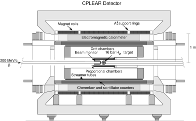
(a)

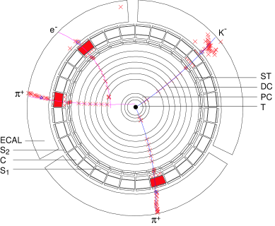
(b)

Figure 1:

(a)	(b)

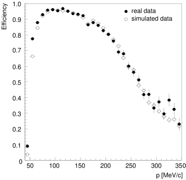
Figure 2:

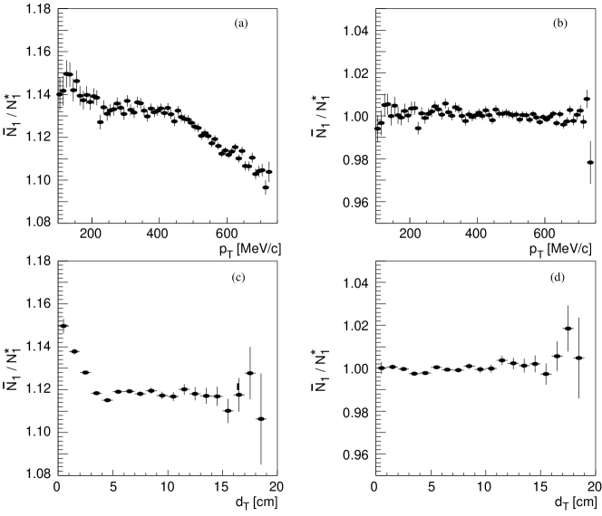
Figure 3:

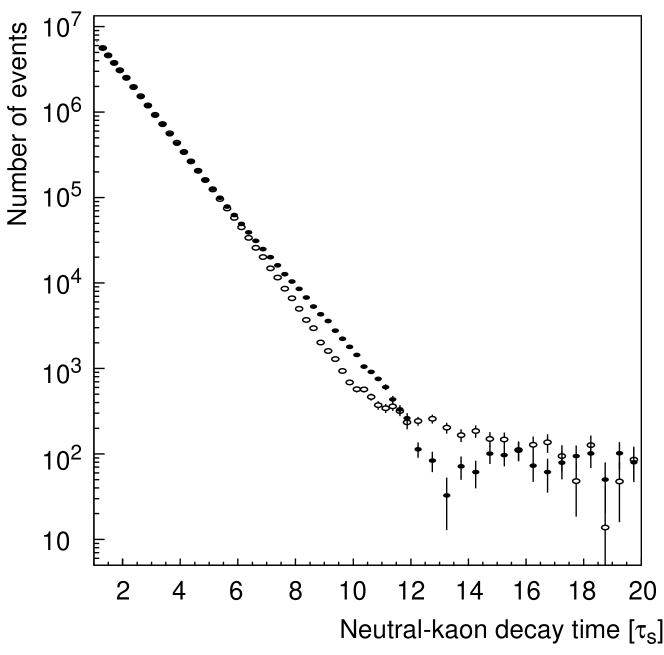
Figure 4:

Figure 5:

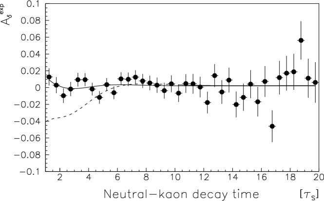
Figure 6:

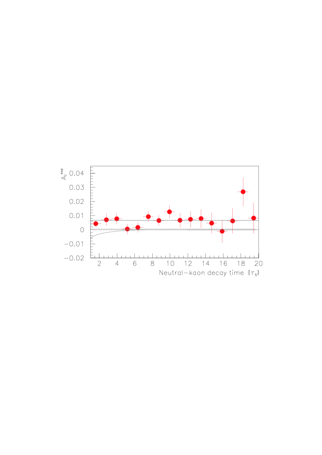
Figure 7:

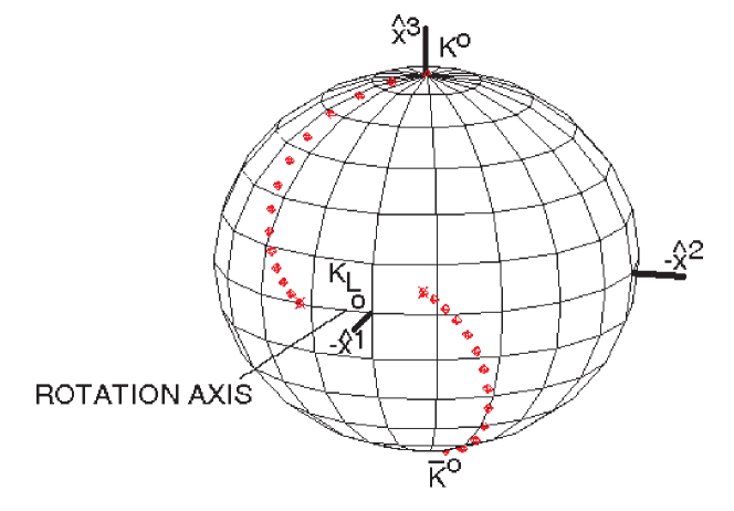
Figure 8:

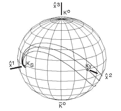
Figure 9:

Figure 10:

Figure 11:

(a)	(b)

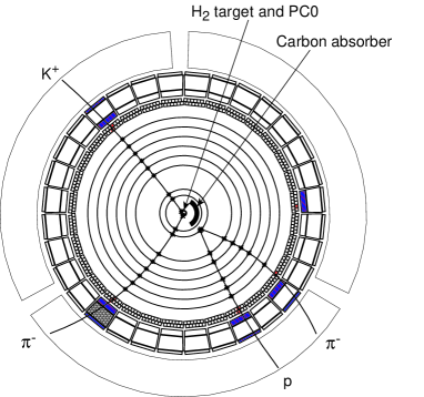
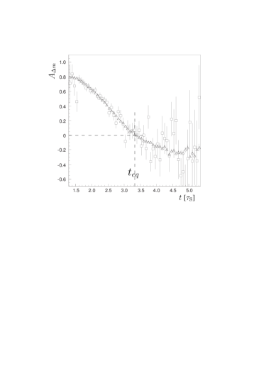
Figure 12:

Figures 1, 2, 5, 6, 7 and 12 have been reprinted with the permission of Elsevier.

Figures 3, 4 and 11 have been reprinted with the permission of Springer.

References

- [1] Jost R 1995 Symmetrie in der Physik Das Märchen vom Elfenbeinernen Turm (Lecture Notes in Physics) m 34 (Berlin: Springer) pp 189–201
- [2] Schwinger J 1951 The theory of quantized fields I Phys. Rev. 82 914–27
- [3] Lüders G L 1954 On the equivalence of invariance under time reversal and under particle-antiparticle conjugation for relativistic field theories K. Dan. Vidensk. Selsk. Mat. Fys. Medd. 28 no 5 pp 1–16
- [4] Pauli W 1955 Exclusion principle, Lorentz group and reflexion of space-time and charge Niels Bohr and the Development of Physics ed L Rosenfeld, V F Weisskopf and W Pauli (London: Pergamon) pp 30–51
- [5] Bell J S 1955 Time reversal in field theory Proc. R. Soc. A 231 479–95
- [6] Jost R 1957 Eine Bemerkung zum CTP-Theorem Helv. Phys. Acta 30 409–16
- [7] Schubert K R et al 1970 The phase of and the invariances CPT and T Phys. Lett. B 31 662–5
- [8] Angelopoulos A et al (CPLEAR collaboration) 1998 First direct observation of time-reversal non-invariance in the neutral-kaon system Phys. Lett. B 444 43–51
- [9] Adler R et al (CPLEAR collaboration) and Ellis J et al 1995 Tests of CPT symmetry and quantum mechanics with experimental data from CPLEAR Phys. Lett. B 364 239–45
- [10] Gell-Mann M and Pais A 1955 Behaviour of neutral particles under charge conjugation Phys. Rev. 97 1387–9
- [11] Pais A and Piccioni O 1955 Note on the decay and absorption of the Phys. Rev. 100 1487-9
-
[12]
Cronin J W 1981 CP symmetry violation – the search for its origin
(Nobel lecture)
Rev. Mod. Phys. 53 3753–83
Christenson J H, Cronin J W, Fitch V L and Turlay R 1964 Evidence for the decay of the K2 meson Phys. Rev. Lett. 13 138–40 - [13] Feynman R P 1961 Theory of Fundamental Processes (New York: Benjamin) ch 9–10
- [14] Kabir P K (ed) 1963 The Development of Weak Interaction Theory (New York: Gordon and Breach)
- [15] Jarlskog C (ed) 1989 CP Violation (Singapore: World Scientific)
- [16] Wolfenstein L (ed) 1989 CP Violation (Amsterdam: North Holland)
- [17] Cahn R N and Goldhaber G 1989 The Experimental Foundations of Particle Physics (Cambridge: Cambridge University Press)
- [18] Tran Thanh Van J (ed) 1990 CP Violation (Gif-sur-Yvette: Editions Frontières)
- [19] Kleinknecht K 2003 Uncovering CP violation (Springer Tracts in Modern Physics 195) (Heidelberg: Springer)
-
[20]
Weisskopf V F and Wigner E P 1930
Berechnung der natürlichen Linienbreite
auf Grund der Diracschen Lichttheorie
Z. Phys. 63 54–73
Weisskopf V F and Wigner E P 1930 Über die natürliche Linienbreite in der Strahlung des harmonischen Oszillators Z. Phys. 65 18–29 - [21] Treiman S B and Sachs R G 1956 Alternate modes of decay of neutral K mesons Phys. Rev. 103 1545–9
- [22] Lee T D, Oehme R and Yang C N 1957 Remarks on possible noninvariance under time reversal and charge conjugation Phys. Rev. 106 340–5
- [23] Lee T D 1981 Particle Physics and Introduction to Field Theory (Chur: Harwood)
- [24] Lavoura L 1991 Phenomenology of the neutral-kaon system in the presence of CPT noninvariance Ann. Phys., NY 207 428–59
- [25] Nakada T 1994 Review on CP Violation Proc. Int. Conf. on Lepton and Photon Interactions (Ithaca, NY) (AIP Conf. Proc. 302) ed P Drell and D Rubin pp 425–63
-
[26]
Lewis R R and Enz C P 1965
Further tests of the violation of CP with neutral K mesons
Phys. Lett. 16 73–5
Enz C P and Lewis R R 1965 On the phenomenological description of CP violation for K-mesons and its consequences Helv. Phys. Acta 38 860–76 Reprinted in Ref.[16] - [27] Alvarez-Gaumé L et al 1999 Violation of time-reversal invariance and CPLEAR measurements Phys. Lett. B 458 347–54
-
[28]
Kabir P K 1970
What is not invariant under time reversal?
Phys. Rev. D 2 540–2; see also:
Aharony A 1970 On separate CPT and T violation checks in the -complex Lett. Nuovo Cimento 3 791–2 - [29] Gerber H-J 2004 Evidence for time-reversal violation? Eur. Phys. J. C 35 195–6
- [30] Wolfenstein L 1999 The search for direct evidence for time reversal violation Int. J. Mod. Phys. E 8 501–11
- [31] Wolfenstein L 1999 Violation of time reversal invariance in decays Phys. Rev. Lett. 83 (1999) 911–2
- [32] Sachs R G 1963 Interference phenomena of neutral K mesons, Ann. Phys., NY 22 239–62
- [33] Lipschutz N R 1966 Invariance principles and the - propagator matrix Phys. Rev. 144 1300–4
- [34] Angelopoulos A et al (CPLEAR collaboration) 2003 Physics at CPLEAR Phys. Rep. 374 165–270
- [35] Buchanan C D et al 1992 Testing CP and CPT violation in the neutral kaon system at a factory Phys. Rev. D 45 4088–107
- [36] Miscetti S (KLOE collaboration) 2004 Highlights of the KLOE experiment at DANE hep-ex/0405040
- [37] Källén G 1964 Elementary Particle Physics (Reading, MA: Addison-Wesley) Deutsche Übersetzung 2. Auflage mit einem ergaenzenden Kapitel von J Steinberger BI, Mannheim, 1974
- [38] Barmin V V et al 1984 CPT symmetry and neutral kaons Nucl. Phys. B 247 283–312
- [39] Angelopoulos A et al (CPLEAR collaboration) 1999 - mass and decay-width differences: CPLEAR evaluation, Phys. Lett. B 471 332–338
- [40] Lai A et al NA48 collaboration) 2005 Search for CP violation in decays Phys. Lett. B 610 165–76 hep-ex/0408053
- [41] Colangelo G et al 2001 scattering, Nucl. Phys. B 603 125–79
- [42] Devlin T J and Dickey J O 1979 Weak hadronic decays: K and K Rev. Mod. Phys. 51 237–50
- [43] Bell J S and Steinberger J 1965 Weak interactions of kaons Proc.of the Oxford Int. Conf. on Elementary Particles ed R G Moorhouse et al pp 195–222
- [44] Steinberger J 1990 Current experimental status of CP violation CP Violation ed J Tran Thanh Van (Gif-sur-Yvette: Editions Frontières) pp 55–92
- [45] Apostolakis A et al (CPLEAR collaboration 1999 Determination of the - and -violation parameters in the neutral-kaon system using the Bell-Steinberger relation and data from CPLEAR Phys. Lett. B 456 297–303
- [46] Dolgov A D and Ponomarev L A 1967 On possible effects of the violation of CP invariance in the radiative decays of neutral K mesons, Sov. J. Nucl. Phys. 4 262–4
- [47] Sehgal L M and L Wolfenstein L 1967 CP-violating interference effects in radiative decays, Phys. Rev. 162 1362–8
- [48] Costa G and Kabir P K 1967 Possible CP-noninvariant effects in decay of neutral kaons Nuovo Cimento A 60 564–9
- [49] Lin Y C R and Valencia G 1988 CP violation in Phys. Rev. D 37 143–8
- [50] Dalitz R H 1951 On an alternative decay process for the neutral -meson Proc. Phys. Soc. A 64 667–9
- [51] Kroll N M and Wada W 1955 Internal pair production associated with the emission of high-energy gamma rays, Phys. Rev. 98 1355–9
- [52] Alavi-Harati A et al (KTEV collaboration) 2000 Observation of CP violation in decays Phys. Rev. Lett. 84 408–11
- [53] Lai A et al (NA48 collaboration) 2003 Investigation of decays Eur. Phys. J. C 30 33–49
- [54] Sehgal L M and van Leusen J 1999 Violation of time reversal invariance in the decays and Phys. Rev. Lett. 83 4933–6
- [55] Perricone M 1998 The Time Machine Fermi News 21 1
- [56] Ellis J and Mavromatos N 1999 Comments on CP, T and CPT violation in neutral kaon decays Phys. Rep. 320 341–54
- [57] Taureg H et al 1976 Study of the photon spectrum in the decay Phys. Lett. B 65 92–6
- [58] Low F E 1958 Bremsstrahlung of very low-energy quanta in elementary particle collisions Phys. Rev. 110 974–7
- [59] Carroll A S et al 1980 Study of the decay Phys. Rev. Lett. 44 529–32
- [60] Wald R 1980 Quantum gravity and time reversibility Phys. Rev. D 21 2742–55
- [61] Page D N 1982 Gen. Relativ. Gravit. 14 299–302
- [62] v. Neumann J 1927 Wahrscheinlichkeitstheoretischer Aufbau der Quantenmechanik Gött. Nach. 245–72
- [63] Pauli W 1990 Die allgemeinen Prinzipien der Wellenmechanik Neu hrsg. von N. Straumann (Berlin: Springer)
- [64] Fano U 1957 Description of states in quantum mechanics by density matrix and operator techniques Rev. Mod. Phys. 29 74–93.
- [65] Hawking S W 1982 The unpredictability of quantum gravity Commun. Math. Phys. 87 395–415
- [66] Ellis J, Hagelin J S, Nanopoulos D V, and Srednicki M 1984 Search for violations of quantum mechanics Nucl. Phys. B 241 381–405
- [67] Gerber H-J 1998 Searching for evolutions of pure states into mixed states in the two-state system Phys. Rev. Lett. 80 2969–71
- [68] Richtmyer R D 1981 Principles of Advanced Mathematical Physics vol 2 (Heidelberg: Springer)
- [69] Feynman R P 1951 An operator calculus having applications in quantum electrodynamics Phys. Rev. 84 108–28
- [70] Gerber H-J 2004 Searching for evolutions from pure states into mixed states with entangled neutral kaons Eur. Phys. J. C 32 229–33
- [71] Huet P and Peshkin M 1995 Violation of CPT and quantum mechanics in the system Nucl. Phys. B 434 3–38
- [72] Man-Duen Choi 1975 Completely positive linear maps on complex matrices Linear Alg. Appl. 10 285–90
- [73] Gorini V, Kossakowski A and Sudarshan E C G 1976 Completely positive dynamical semigroups of N-level systems J. Math. Phys. 17 821–5
- [74] Benatti F and Floreanini R 1997 Completely positive dynamical maps and the neutral kaon system Nucl. Phys. B 488 335–63
- [75] Benatti F, Floreanini R and Romano R 2002 Complete positivity and entangled degrees of freedom J. Phys. A: Math. Gen. 35 4955-72
- [76] Adler R et al (CPLEAR collaboration) 1997 Experimental determination of / ratio in antiproton annihilations at rest in gaseous hydrogen at 15 and 17 bar Phys. Lett. B 403 383–9
- [77] Alicki R and Lendi K 1987 Quantum Dynamical Semigroups and Applications (Lecture Notes in Physics 286) (Berlin: Springer)
- [78] Benatti F and Floreanini R 1998 Completely positive dynamics of correlated neutral kaons Nucl. Phys. B 511 550–76
- [79] Goldhaber M, Lee T D and Yang C N 1958 Decay modes of a system Phys. Rev. 112 1796–8
- [80] Lipkin H J 1968 CP violation and coherent decays of kaon pairs Phys. Rev. 176 1715–8
- [81] Maiani L 1995 CP and CPT violation in neutral kaon decays The Second DANE Physics Handbook ed L Maiani et al (Frascati: INFN) pp 3-26
- [82] Ellis J, Lopez J L, Mavromatos N E and Nanopoulos D V 1996 Precision tests of CPT symmetry and quantum mechanics in the neutral kaon system Phys. Rev. D 53 3846–70
- [83] Benatti F and Floreanini R 1997 Experimental limits on complete positivity from the system Phys. Lett. B 401 337–46
- [84] Bernabeu J, Mavromatos N E and Papavassiliou J 2004 Novel type of CPT violation for correlated Einstein-Podolsky-Rosen states of neutral mesons Phys. Rev. Lett. 92 131601-1–4 hep-ph/0310180
- [85] Good M L 1957 Relation between scattering and absorption in the Pais-Piccioni experiment Phys. Rev. 106 591–5
- [86] Kleinknecht K 1973 - regeneration Fortschritte der Physik 21 57–84
- [87] Burkhardt H et al. (NA31 collaboration) 1988 First evidence for direct CP violation Phys. Lett. B 206 169–76
- [88] Batley J R et al (NA48 collaboration) 2002 A precision measurement of direct CP violation in the decay of neutral kaons into two pions Phys. Lett. B 544 97–112
- [89] Banner D et al 1973 Experimental comparison of CP violation in and decays Phys. Rev. D 7 1989–99
- [90] Niebergall F et al 1974 Experimental study of the rule in the time-dependent rate of Phys. Lett. B 49 103–8
- [91] Apostolakis A et al (CPLEAR collaboration) 1998 An EPR experiment testing the non-separability of the wave-function Phys. Lett. B 422 339–48
- [92] Gabathuler E and Pavlopoulos P 1984 Strong and Weak CP violation at LEAR Proc. of the Workshop on Physics at LEAR with Low Energy Cooled Antiprotons (Erice 1982) (New York: Plenum) pp 747–59
- [93] Fetscher W et al 1996 Regeneration of arbitrary coherent neutral kaon states: A new method for measuring the - forward scattering amplitude Z. Phys. C 72 543–7
- [94] Adler R et al (CPLEAR collaboration) 1996 The CPLEAR detector at CERN Nucl. Instrum. Methods A 379 76–100
-
[95]
Baird S et al 1998
Overview of the recent operation of the AAC and LEAR for
the low-energy antiproton physics programme
Proc. of the 1997 Particle Accelerator Conference (Vancouver)
ed M Comyn et al (Piscataway: IEEE) pp 982–4
Koziol H and Möhl D 2004 The CERN low-energy antiproton programme: the synchrotrons Phys. Rep. 403-404 271–80 - [96] Angelopoulos A et al (CPLEAR collaboration) 1997 Measurement of neutral kaon regeneration amplitudes in carbon at momenta below 1 GeV/ Phys. Lett. B 413 422–30
- [97] Apostolakis A et al (CPLEAR collaboration) 2000 A detailed description of the analysis of the decay of neutral kaons to in the CPLEAR experiment Eur. Phys. J. C 18 41–55
- [98] Caso C et al (Particle Data Group) Eur. Phys. J. C 3 1
- [99] Angelopoulos A. et al (CPLEAR collaboration) 1998 A determination of the CPT violation parameter Re() from the semileptonic decay of strangeness-tagged neutral kaons Phys. Lett. B 444 52–60
- [100] Eidelman S et al (Particle Data Group) 2004 Phys. Lett. B 592 1
- [101] Dorfan D et al 1967 Charge asymmetry in the muonic decay of the K2 Phys. Rev. Lett. 19 987–93
- [102] Bennett S et al 1967 Measurement of the charge asymmetry in the decay Phys. Rev. Lett. 19 993–7
- [103] Alavi-Harati A et al (KTEV collaboration) 2002 Measurement of the charge asymmetry Phys. Rev. Lett. 88 181601-1–5
- [104] Ruggiero G 2003 Measurement of the charge asymmetry in the Ke3 decay of using the NA48 detector PhD Thesis Università di Firenze
- [105] Angelopoulos A et al (CPLEAR collaboration) 1998 Measurement of the - mass difference using semileptonic decays of tagged neutral kaons Phys. Lett. B 444 38–42
- [106] Angelopoulos A et al (CPLEAR collaboration) 2001 -violation and -invariance measurements in the CPLEAR experiment: a detailed description of the analysis of neutral-kaon decays to Eur. Phys. J. C 22 55–79
- [107] Alavi-Harati A et al (KTEV collaboration) 2003 Measurement of direct CP violation, CPT symmetry, and other parameters in the neutral kaon system Phys. Rev. D 67 012005-1–33 Phys. Rev. D 70 079904(E)
- [108] Wolfenstein L and Trippe T G in Ref. [100]
- [109] Geweniger G et al 1974 A new determination of the decay parameters Phys. Lett. B 48 487–91
- [110] Bell J S 1964 On the Einstein Podolski Rosen paradox Physics 1 195–200
- [111] Di Domenico A 1995 Testing quantum mechanics in the neutral kaon system at a factory Nucl. Phys. B 450 293–324
- [112] Dalitz R H and Garbarino G 2001 Local realistic theories and quantum mechanics for the two-neutral-kaon system Nucl. Phys. B 206 483–517 quant-ph/0011108
- [113] Dass G V and Grimus W 2001 Testing the Wigner-Weisskopf approximation by using neutral-meson-antimeson correlated states Phys. Lett. B 521 267–72 hep-ph/010904
- [114] Urbanowski K 2004 A new interpretation of one CPT violation test for - system Acta Physica Polonica B 35 2069–83 hep-ph/0202253
- [115] Tanner N W and Dalitz R H 1986 The determination of T- and CPT-violations for the (,) complex by /comparisons Ann. Phys., NY 171 463–88
- [116] Bjork G, Soderholm J, Trifonov A, Tsegaye T and Karlsson A 1999 Complementarity and the uncertainty relations Phys. Rev. A 60 1874–82
- [117] Bramon A, Garbarino G and Hiesmayr B C 2004 Quantitative complementarity in two-path interferometry Phys. Rev. A 69 022112-1–5 quant-ph/0311179
- [118] Bramon A, Garbarino G and Hiesmayr B C 2004 Quantum marking and quantum erasure for neutral kaons Phys. Rev. Lett. 92 020405-1–4 hep-ph/0311232
- [119] Barenboim G and Mavromatos N E 2005 CPT violating decoherence and LSND: a possible window to Planck scale physics JHEP 0501 034-1–24 hep-ph/0404014
- [120] Jauch J M and Rohrlich F 1955 The Theory of Photons and Electrons (Reading, MA: Addison-Wesley)
- [121] Angelopoulos A et al (CPLEAR collaboration) 2001 transitions monitored by strong interactions: a new determination of the - mass difference Phys. Lett. B 503 49–57