IPPP/06/15

DCPT/06/30

March 2006

Scattering amplitudes with massive fermions using BCFW recursion

K.J. Ozeren and W.J. Stirling

Institute for Particle Physics Phenomenology,

University of Durham, DH1 3LE, UK

We study the QCD scattering amplitudes for $\bar{q}q\to gg$ and $\bar{q}q\to ggg$ where $q$ is a massive fermion. Using a particular choice of massive fermion spinor we are able to derive very compact expressions for the partial spin amplitudes for the $2\to 2$ process. We then investigate the corresponding $2\to 3$ amplitudes using the BCFW recursion technique. For the helicity conserving partial amplitudes we again derive very compact expressions, but were unable to treat the helicity-flip amplitudes recursively, except for the case where all the gluon helicities are the same. We therefore evaluate the remaining partial amplitudes using standard Feynman diagram techniques.

1 Introduction

In the last two years there has been dramatic progress in the calculation of multi-particle scattering amplitudes in quantum field theory. Following Witten’s [1] discovery of a connection between QCD amplitudes and twistor string theory, a calculational technique [2] was found which has come to be known as ‘the CSW construction’. It amounts to an effective scalar perturbation theory, in which MHV amplitudes are elevated to the status of vertices, connected by scalar propagators. This scheme found wide application [3, 4, 5, 6, 7, 8], though it turned out that there was an even more efficient way to calculate scattering amplitudes. Britto, Cachazo, Feng and Witten found a recursion relation [9, 10] which, by shifting momenta, takes advantage of the analytic properites of tree amplitudes. Use of the BCFW recursion relation led easily to very compact expressions. Originally applied to purely gluonic tree amplitudes, the recursion has since been extended to include fermions [11, 12], gravitons [13] and loop amplitudes [14, 15, 16, 17]. As well as perhaps giving hints of as yet unknown mathematical structure beyond the Standard Model, these developments are potentially important for the calculation of Standard Model backgrounds at colliders such as the LHC. The more accurately the relevant cross sections are known, the higher the discovery potential of the machine will be.

One area of very recent progress is the calculation of amplitudes involving massive fermions. It was shown in Ref. [18] how to generalize Supersymmetric Ward Identities [19] to include massive particles. In this way, different amplitudes involving fields belonging to the same supersymmetric multiplet are related by a rotation. For instance [20], amplitudes involving quarks and gluons are related by SWIs to amplitudes involving scalars and gluons, and these have been calculated in Ref. [21]. The off-shell Berends-Giele [22] recursion has also proved useful [23]. Tree amplitudes with massive fermions are required as input within the unitarity [24] method to calculate one-loop amplitudes, and to this end Ref. [25] provides four- and five-point amplitudes with D-dimensional fermions, calculated using BCFW recursion.

The recursion relations were extended in Ref. [26] to include massive fermions, and in [27] four-point amplitudes involving two massive quarks and two gluons were calculated. The topic of the present work is to extend this to five-point amplitudes, using a treatment of massive fermion spinors introduced some twenty years ago in Ref. [28]. We first outline the particular spinor helicity method we will use, and then we show that $2\to 2$ scattering processes in QCD can be written in a form which is ideally suited for use in BCFW recursion. In Section 4 we use the recursion relations to derive compact expressions for certain $\bar{q}q\to ggg$ partial amplitudes. Those partial amplitudes which we could not treat recursively are evaluated using Feynman diagrams in Section 5. Finally, we present our conclusions.

2 Spinor Products

For many years amplitudes involving massless momenta $p_{i}$ and $p_{j}$ have been expressed in terms of spinor products,

$$[ij]=\bar{u}^{+}(p_{i})u^{-}(p_{j})\hskip 14.22636pt\mbox{and}\hskip 14.22636pt\langle ij\rangle=\bar{u}^{-}(p_{i})u^{+}(p_{j}).$$ (2.1)

In this way amplitudes find their simplest expression. The spinors in question can be thought of either as two-component Weyl or 4-component Dirac spinors. Numerical evaluation of such amplitudes involves the use of the standard formulae for the spinor products in terms of the momentum 4-vectors. Following [28], let us first introduce two 4-vectors $k_{0}$ and $k_{1}$ such that

$$k_{0}\cdot k_{0}=0\hskip 5.69054pt,\hskip 5.69054ptk_{1}\cdot k_{1}=-1\hskip 5.69054pt,\hskip 5.69054ptk_{0}\cdot k_{1}=0.$$ (2.2)

We now define a basic spinor $u_{-}(k_{0})$ via

$$u^{-}(k_{0})\bar{u}^{-}(k_{0})=\frac{1-\gamma^{5}}{2}{\raise 0.97221pt\hbox to5.52084pt{\hss/\hss}\hbox to0.0pt{\hss$k$}}_{0},$$ (2.3)

and choose the corresponding positive helicity state to be

$$u^{+}(k_{0})={\raise 0.97221pt\hbox to5.52084pt{\hss/\hss}\hbox to0.0pt{\hss$k$}}_{1}u^{-}(k_{0}).$$ (2.4)

Using these definitions it is possible to construct spinors for any null momentum $p$ as follows:

$$u^{\lambda}(p)=\frac{{\raise-1.31944pt\hbox to5.03125pt{\hss/\hss}\hbox to0.0pt{\hss$p$}}\ u^{-\lambda}(k_{0})}{\sqrt{2p\cdot k_{0}}},$$ (2.5)

with $\lambda=\pm$. Note that this satisfies the massless Dirac equation ${\raise-1.31944pt\hbox to5.03125pt{\hss/\hss}\hbox to0.0pt{\hss$p$}}u(p)=0$, as required. We can now simply evaluate spinor products. For example,

$$[ij] = \bar{u}^{+}(p_{i})u^{-}(p_{j})$$ (2.6)

$$= \frac{\bar{u}^{-}(k_{0})\ {\raise-1.31944pt\hbox to6.96053pt{\hss/\hss}\hbox to0.0pt{\hss$p_{i}$}}\ {\raise-1.815pt\hbox to7.65793pt{\hss/\hss}\hbox to0.0pt{\hss$p_{j}$}}\ u^{+}(k_{0})}{\sqrt{4\ (p_{i}\cdot k_{0})(p_{j}\cdot k_{0})}}$$ (2.7)

$$= \frac{\mbox{Tr}(\frac{(1-\gamma^{5})}{2}\ {\raise 0.06999pt\hbox to8.32085pt{\hss/\hss}\hbox to0.0pt{\hss$k_{0}$}}\ {\raise-1.31944pt\hbox to6.96053pt{\hss/\hss}\hbox to0.0pt{\hss$p_{i}$}}\ {\raise-1.815pt\hbox to7.65793pt{\hss/\hss}\hbox to0.0pt{\hss$p_{j}$}}\ {\raise 0.06999pt\hbox to8.32085pt{\hss/\hss}\hbox to0.0pt{\hss$k_{1}$}})}{\sqrt{4\ (p_{i}\cdot k_{0})(p_{j}\cdot k_{0})}}$$ (2.8)

$$= \frac{(p_{i}\cdot k_{0})(p_{j}\cdot k_{1})-(p_{j}\cdot k_{0})(p_{i}\cdot k_{1})-i\epsilon_{\mu\nu\rho\sigma}k_{0}^{\mu}p_{i}^{\nu}p_{j}^{\rho}k_{1}^{\sigma}}{\sqrt{(p_{i}\cdot k_{0})(p_{j}\cdot k_{0})}}.$$ (2.9)

A similar expression is obtained for the angle product $\langle ij\rangle$. The arbitrary $k_{0}$ and $k_{1}$ can now be chosen so as to yield as simple an expression for the product $[ij]$ and $\langle ij\rangle$ as possible, to facilitate numerical evaluation of the ampitudes. The choice

$$k_{0}=(1,0,0,1)$$ (2.10)

$$k_{1}=(0,0,1,0)$$ (2.11)

is a good one, giving the familiar

$$[ij]=(p_{i}^{y}+ip_{i}^{x})\left[\frac{p_{j}^{0}-p_{j}^{z}}{p_{i}^{0}-p_{i}^{z}}\right]^{\frac{1}{2}}-(p_{j}^{y}+ip_{j}^{x})\left[\frac{p_{i}^{0}-p_{i}^{z}}{p_{j}^{0}-p_{j}^{z}}\right]^{\frac{1}{2}}.$$ (2.12)

2.1 Massive spinors

To evaluate spinor products involving massive spinors, we need to find a definition analogous to (2.5). One possibility is that outlined in [28],

$$u^{\lambda}(p)=\frac{({\raise-1.31944pt\hbox to5.03125pt{\hss/\hss}\hbox to0.0pt{\hss$p$}}+m)u^{-\lambda}(k_{0})}{\sqrt{2p\cdot k_{0}}},$$ (2.13)

which satisfies the massive Dirac equation, $({\raise-1.31944pt\hbox to5.03125pt{\hss/\hss}\hbox to0.0pt{\hss$p$}}-m)u^{\lambda}(p)=0$. The $m$ in (2.13) is positive or negative when $u^{\lambda}(p)$ describes a particle or antiparticle respectively. This definition has the virtue of being smooth in the limit $m\to 0$. We will use (2.13) to evaluate products involving massive spinors.

It is easily seen that the familiar $[.\ .]$ and $\langle.\ .\rangle$ products take the same form for massive spinors as they do for massless ones. Explicit mass terms drop out due to various trace theorems. However, the product of like-helicity spinors is now non-zero:

$$(ij) = \bar{u}^{\pm}(p_{i})u^{\pm}(p_{j}),$$ (2.14)

$$= m_{i}\left(\frac{p_{j}\cdot k_{0}}{p_{i}\cdot k_{0}}\right)^{\frac{1}{2}}+i\leftrightarrow j$$ (2.15)

$$= m_{i}\left(\frac{p_{j}^{0}-p_{j}^{z}}{p_{i}^{0}-p_{i}^{z}}\right)^{\frac{1}{2}}+i\leftrightarrow j,$$ (2.16)

where in the last line we have used $k_{0}$ as given in (2.10). Note that the like-helicity product is the same whatever the helicity of the spinors involved, and that we use a round bracket as a shorthand notation for it.

We have been using the word ‘helicity’ to refer to the spin projection of massive fermions, but in fact this is only justified if the projection is onto the direction of the momentum vector, and it is not obvious that this is the case. There exists a unique polarization vector, though it depends on the arbitrary $k_{0}$,

$$\sigma^{\mu}=\frac{1}{m}\left(p^{\mu}-\frac{m^{2}}{p\cdot k_{0}}k_{0}^{\mu}\right).$$ (2.17)

The spinors (2.13) satisfy

$$\big{(}1-\lambda\gamma^{5}{\raise-0.34723pt\hbox to5.71413pt{\hss/\hss}\hbox to0.0pt{\hss$\sigma$}}\big{)}u^{\lambda}=0.$$ (2.18)

We see that besides the momentum $p$ there is an additional contribution to the polarization vector proportional to $k_{0}$. Suppose we have an anti-fermion $i$ and fermion $j$ in the initial state and they approach along the $z$ axis, in the positive and negative directions respectively. If we choose $k_{0}$ to be a unit vector in the $z$ direction, i.e.

$$k_{0}=\big{(}1,0,0,1\big{)},$$ (2.19)

then for momenta

$$p_{i} = \big{(}E,0,0,\beta E\big{)},$$ (2.20)

$$p_{j} = \big{(}E,0,0,-\beta E\big{)},$$ (2.21)

we have the following polarization vectors:

$$\sigma_{i}^{\mu} = \frac{1}{m_{i}}\big{(}-E\beta,0,0,-E\big{)},$$ (2.22)

$$\sigma_{j}^{\mu} = \frac{1}{m_{j}}\big{(}E\beta,0,0,-E\big{)}.$$ (2.23)

If we recall that $m_{i}$ is negative because $i$ is an antiparticle, then we see that each polarization vector points in the same direction as the corresponding momentum, so that the spinors $u^{\lambda}(p)$ are indeed helicity eigenstates for this choice of $k_{0}$. However, choosing $k_{0}$ to be parallel to one of the particle’s momenta results, in the massless limit, in the denominators of products such as that in (2.16) vanishing. By being careful to take the limit algebraically this does not present a problem. But it should be noted that in such cases products like $(ij)$ do not necessarily vanish in the massless limit. We can sidestep this issue by choosing a different $k_{0}$, though we could not then talk of the helicity of the fermion.

2.2 Example: $\bar{q}q\to gg$

To demonstrate the use of the massive spinor products described in the previous section we calculate the helicity amplitudes $M^{\lambda_{1}\lambda_{2}\lambda_{3}\lambda_{4}}$ for the simple QCD process $\bar{q}^{\lambda_{1}}(p_{1})\ q^{\lambda_{2}}(p_{2})\to g^{\lambda_{3}}(p_{3})\ g^{\lambda_{4}}(p_{4})$. The $\lambda_{1},\lambda_{2}=\pm$ labels on the quarks refer to their spin polarizations in the sense already indicated. If we choose $k_{0}$ appropriately then they can be thought of as helicity labels. We will evaluate the partial (colour) amplitudes for the above scattering process, i.e. we consider contributions only from those diagrams with a particular ordering of the external gluons. The full colour-summed amplitudes can then be recovered by inserting appropriate colour factors, as described in Appendix B.

We first consider the $M^{+-+-}$ partial amplitude, for which there are two Feynman diagrams, shown in Figure 1. We will express them in terms of massive spinor products. For the slashed gluon polarization vectors we use

$${\raise-0.34723pt\hbox to4.05904pt{\hss/\hss}\hbox to0.0pt{\hss$\epsilon$}}^{+}(p,k) = \sqrt{2}\ \frac{u_{+}(k)\bar{u}_{+}(p)+u_{-}(p)\bar{u}_{-}(k)}{\langle kp\rangle},$$ (2.24)

$${\raise-0.34723pt\hbox to4.05904pt{\hss/\hss}\hbox to0.0pt{\hss$\epsilon$}}^{-}(p,k) = \sqrt{2}\ \frac{u_{+}(p)\bar{u}_{+}(k)+u_{-}(k)\bar{u}_{-}(p)}{[pk]},$$ (2.25)

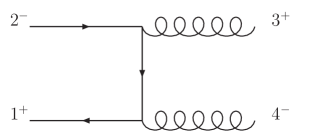
(a) Diagram A

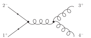
(b) Diagram B

Figure 1: Diagrams contributing to the colour-ordered partial amplitude for the process $\bar{q}^{+}(p_{1})q^{-}(p_{2})\to g^{+}(p_{3})g^{-}(p_{4})$.

where $k$ is a (null) reference vector which may be chosen separately for each gluon. Different choices of reference vector amount to working in different gauges. The choice $k_{3}=p_{4}$ and $k_{4}=p_{3}$ is particularly convenient in this context, as Diagram B vanishes in this gauge. We have for the other diagram

$$\bar{u}^{+}(p_{1})\ \frac{{\raise-0.34723pt\hbox to4.05904pt{\hss/\hss}\hbox to0.0pt{\hss$\epsilon$}}^{-}(p_{4})}{\sqrt{2}}\ \frac{{\raise-1.31944pt\hbox to7.83125pt{\hss/\hss}\hbox to0.0pt{\hss$p_{2}$}}-{\raise-1.31944pt\hbox to7.83125pt{\hss/\hss}\hbox to0.0pt{\hss$p_{3}$}}+m}{(p_{2}-p_{3})^{2}-m^{2}}\ \frac{{\raise-0.34723pt\hbox to4.05904pt{\hss/\hss}\hbox to0.0pt{\hss$\epsilon$}}^{+}(p_{3})}{\sqrt{2}}\ u^{-}(p_{2}),$$ (2.26)

which simplifies easily to

$$\bar{u}^{+}(p_{3}){\raise-1.31944pt\hbox to7.83125pt{\hss/\hss}\hbox to0.0pt{\hss$p_{2}$}}u^{+}(p_{4})\ \frac{\bar{u}^{+}(p_{1})\big{[}u^{-}(p_{3})\bar{u}^{-}(p_{4})+u^{+}(p_{4})\bar{u}^{+}(p_{3})\big{]}u^{-}(p_{2})}{4\ p_{3}\cdot p_{4}\ p_{4}\cdot p_{1}},\\$$ (2.27)

so that

$$M^{+-+-}=[3|2|4\rangle\frac{[13](42)+(14)[32]}{4\ p_{3}\cdot p_{4}\ p_{4}\cdot p_{1}}.$$ (2.28)

As promised, we are left with an expression for the amplitude in terms of vector products and massive spinor products.

We next consider the other $M^{\lambda_{1}\lambda_{2}+-}$ amplitudes. It is interesting to note that these are directly obtained from the $M^{+-+-}$ amplitude simply by changing the type of certain brackets. Thus

$$M^{+++-} = [3|2|4\rangle\frac{[13]\langle 42\rangle+(14)(32)}{4\ p_{3}\cdot p_{4}\ p_{4}\cdot p_{1}},$$ (2.29)

$$M^{--+-} = [3|2|4\rangle\frac{(13)(42)+\langle 14\rangle[32]}{4\ p_{3}\cdot p_{4}\ p_{4}\cdot p_{1}},$$ (2.30)

$$M^{-++-} = [3|2|4\rangle\frac{(13)\langle 42\rangle+\langle 14\rangle(32)}{4\ p_{3}\cdot p_{4}\ p_{4}\cdot p_{1}}.$$ (2.31)

Those amplitudes where the gluons have helicities $(-\ +)$ can be obtained directly from the ones above by complex conjugation.

Let us now examine the case where the gluons have the same helicity. By direct calculation we find

$$M^{--++}=m[43]\frac{\langle 13\rangle(42)-\langle 14\rangle(32)}{\langle 34\rangle^{2}\ 2\ p_{4}\cdot p_{1}}.$$ (2.32)

from which we deduce

$$M^{++++} = m[43]\frac{(13)\langle 42\rangle-(14)\langle 32\rangle}{\langle 34\rangle^{2}\ 2\ p_{4}\cdot p_{1}},$$ (2.33)

$$M^{+-++} = 0,$$ (2.34)

$$M^{-+++} = m[43]\frac{\langle 13\rangle\langle 42\rangle-\langle 14\rangle\langle 32\rangle}{\langle 34\rangle^{2}\ 2\ p_{4}\cdot p_{1}},$$ (2.35)

$$= \frac{m[34]\langle 12\rangle}{\langle 34\rangle\ 2\ p_{4}\cdot p_{1}},$$ (2.36)

where in the last line we have used the Schouten identity. The amplitudes with two negative helicity gluons are obtained via complex conjugation. There are several interesting things to note about these results. First, the amplitude $M^{+-++}$ vanishes (for any choice of $k_{0}$) because of the identity $(13)(42)-(14)(32)=0$. Second, when $k_{0}$ is parallel to the line of approach of the fermions (i.e. when we work in the helicity basis) then the product $\langle 12\rangle$, and hence $M^{-+++}$, vanishes.

We have verified that when squared and summed over spins and colours, the set of $2\to 2$ scattering amplitudes given above matches the well-known result (see for example Ref. [29]) calculated using Feynman diagrams and ‘trace technology’, namely

$$\sum_{\mbox{\tiny{colours}}}\sum_{\mbox{\tiny{spins}}}|M|^{2}=256\ \left(\frac{1}{6\tau_{1}\tau_{2}}-\frac{3}{8}\right)\left(\tau_{1}^{2}+\tau_{2}^{2}+\rho-\frac{\rho^{2}}{4\tau_{1}\tau_{2}}\right),$$ (2.37)

where

$$\tau_{1}=\frac{2p_{1}\cdot p_{3}}{s},\hskip 14.22636pt\tau_{2}=\frac{2p_{1}\cdot p_{4}}{s},\hskip 14.22636pt\rho=\frac{4m^{2}}{s},\hskip 14.22636pts=(p_{1}+p_{2})^{2}.$$ (2.38)

Finally, the $m\to 0$ behaviour of the spin amplitudes can easily be read off from the expressions given above. For example, if $E$ denotes the typical scale of the $2\to 2$ scattering, then in the $m/E\to 0$ limit we have

$$M^{++\pm\mp},\ M^{--\pm\mp} \sim O(1),$$

$$M^{+-\pm\mp},\ M^{-+\mp\pm} \sim O(m/E),$$

$$M^{++\pm\pm},\ M^{--\mp\mp} \sim O(m^{2}/E^{2}),$$

$$M^{+---},\ M^{-+++} \sim O(m/E),$$

$$M^{+-++},\ M^{-+--} = 0.$$ (2.39)

Note that in deriving these results we have assumed that $k_{0}$ is not directed along any of the particle momenta, so that all $(ij)$ spinor products are $O(m)$ in the $m\to 0$ limit, and $\langle ij\rangle$, $[ij]$ products are $O(E)$. If on the other hand we choose the (fermion) helicity basis by taking $k_{0}$ in the direction of (say) $p_{1}$, then (2.39) becomes

$$M^{+-\pm\mp},\ M^{-+\mp\pm} \sim O(1),$$

$$M^{+-\pm\pm},\ M^{-+\mp\mp} = 0,$$

$$M^{++\pm\mp},\ M^{--\mp\pm} \sim O(m/E),$$

$$M^{++++},\ M^{----} \sim O(m/E),$$

$$M^{--++},\ M^{++--} \sim O(m^{3}/E^{3}).$$ (2.40)

3 BCFW Recursion

In Ref. [9] Britto, Cachazo and Feng introduced new recursion relations for amplitudes involving gluons. The recursion involved on-shell amplitudes with momenta shifted by a complex amount. Later [10], the same authors with Witten gave an impressively simple and general proof of the recursion relations. They have since been successfully applied to amplitudes involving fermions [11, 12] and gravitons [13]. Risager [30] has demonstrated how they are related to the earlier ‘MHV rules’, providing a proof of the latter simply using BCF recursion. There has also been much progress at 1-loop level [14, 15, 16, 17], which has dovetailed nicely with the earlier unitarity work [24].

We begin by choosing two (massless) particles $i$ and $j$ whose slashed momenta we shift as follows,

$${\raise-1.31944pt\hbox to5.03125pt{\hss/\hss}\hbox to0.0pt{\hss$p$}}_{i}\to\hat{{\raise-1.31944pt\hbox to5.03125pt{\hss/\hss}\hbox to0.0pt{\hss$p$}}_{i}} = {\raise-1.31944pt\hbox to5.03125pt{\hss/\hss}\hbox to0.0pt{\hss$p$}}_{i}+z{\raise-1.31944pt\hbox to4.9653pt{\hss/\hss}\hbox to0.0pt{\hss$\eta$}},$$

$${\raise-1.31944pt\hbox to5.03125pt{\hss/\hss}\hbox to0.0pt{\hss$p$}}_{j}\to\hat{{\raise-1.31944pt\hbox to5.03125pt{\hss/\hss}\hbox to0.0pt{\hss$p$}}_{j}} = {\raise-1.31944pt\hbox to5.03125pt{\hss/\hss}\hbox to0.0pt{\hss$p$}}_{j}-z{\raise-1.31944pt\hbox to4.9653pt{\hss/\hss}\hbox to0.0pt{\hss$\eta$}},$$ (3.1)

where

$${\raise-1.31944pt\hbox to4.9653pt{\hss/\hss}\hbox to0.0pt{\hss$\eta$}}=u^{+}(p_{j})\bar{u}^{+}(p_{i})+u^{-}(p_{i})\bar{u}^{-}(p_{j})$$ (3.2)

is such that both $p_{i}$ and $p_{j}$ remain on-shell. Using the familiar spin-sum condition,

$$\sum_{\lambda}u^{\lambda}(p)\ \bar{u}^{\lambda}(p)={\raise-1.31944pt\hbox to5.03125pt{\hss/\hss}\hbox to0.0pt{\hss$p$}}$$ (3.3)

we can re-express the shift (3.1) as a shift of spinors:

$$u^{+}(p_{i}) \to u^{+}(\widehat{p_{i}})=u^{+}(p_{i})+z\ u^{+}(p_{j})$$ (3.4)

$$\bar{u}^{-}(p_{i}) \to \bar{u}^{-}(\widehat{p_{i}})=\bar{u}^{-}(p_{i})+z\ \bar{u}^{-}(p_{j})$$ (3.5)

$$\bar{u}^{+}(p_{j}) \to \bar{u}^{+}(\widehat{p_{j}})=\bar{u}^{+}(p_{j})-z\ u^{+}(p_{i})$$ (3.6)

$$u^{-}(p_{j}) \to u^{-}(\widehat{p_{j}})=u^{-}(p_{j})-z\ u^{-}(p_{i}).$$ (3.7)

In the Weyl spinor notation we are shifting $\lambda_{i}$ and $\tilde{\lambda}_{j}$. For massless particles, Dirac 4-spinors are effectively two copies of a Weyl 2-spinor, hence the four shifts of (3.4)–(3.7). Notice that there is no symmetry between $i$ and $j$ — they are treated differently.

The amplitude is now a complex function of the parameter $z$. What the authors of [10] showed was that we can use the analytic properties of the amplitude as a function of $z$ to glean information about the physical case $z=0$. In particular, we get a recursion relation, which can be stated as

$$A_{n}=\sum_{\mbox{\tiny{partitions}}}\sum_{\mbox{\tiny{s}}}A_{L}(\widehat{p}_{i},\widehat{P}^{-s})\ \frac{1}{P^{2}-m_{P}^{2}}\ A_{R}(-\widehat{P}^{s},\widehat{p}_{j}).$$ (3.8)

where the hatted quantities are the shifted momenta. In fact, this is only valid if the helicities of the marked particles are chosen appropriately. The crucial property which must be retained if (3.8) is to hold is that the shifted amplitude must vanish in the limit $z\to\infty$. There are rules [10, 11, 26, 27] detailing which marking prescriptions are permitted in different cases. For our purposes, we will be on safe ground if the shifted gluons have helicites $(h^{i},h^{j})=(+,-)$ or $(\pm,\pm)$.

This method of calculation is particularly efficient because much of the computational complexity encountered in a Feynman diagram calculation is avoided since the lower point amplitudes $A_{L}$ and $A_{R}$ can be maximally simplified before being inserted in (3.8).

The sum is over all partitions of the particles into a ‘left’ group and a ‘right’ group, subject to the requirement that particles $i$ and $j$ are on opposite sides of the divide. The sum over $s$ is a sum over the spins of the internal particle. Each diagram is associated with a particular value for the complex parameter $z$, which can be found via the condition that the internal momentum $\widehat{P}$ is on-shell. Note that $\widehat{P}$ is always a function of $z$ because of the restriction that the marked particles $i$ and $j$ appear on opposite sides of the divide.

One useful point to note in practice is that three-point gluon vertices vanish for certain marking choices. In particular, for the $j$ side of the diagram a gluon vertex with helicites $(++-)$ vanishes, as does the combination $(--+)$ on the $i$ side. This was pointed out in Ref. [9].

We will be concerned in this work with the process $\bar{q}q\to ggg$, and so will encounter recursive diagrams connected by an internal fermion, the propagator of which is, in this formalism, the same as that of a scalar. Following Ref. [27], we ‘strip’ fermions from the lower point amplitudes which feed the recursion and write

$$A_{n} = \sum_{\mbox{\tiny{partitions}}}\sum_{\mbox{\tiny{s}}}A_{L}(\widehat{p}_{i},\widehat{P}^{*})\ \frac{u_{s}(\widehat{P})\bar{u}_{s}(\widehat{P})}{P^{2}-m_{P}^{2}}\ A_{R}(-\widehat{P}^{*},\widehat{p}_{j}),$$ (3.9)

$$= \sum_{\mbox{\tiny{partitions}}}A_{L}(\widehat{p}_{i},\widehat{P}^{*})\ \frac{{\raise 1.11111pt\hbox to5.55557pt{\hss/\hss}\hbox to0.0pt{\hss$\widehat{P}$}}+m_{P}}{P^{2}-m_{P}^{2}}\ A_{R}(-\widehat{P}^{*},\widehat{p}_{j}).$$ (3.10)

where $P^{*}$ shows that the amplitude has been stripped of this external spinor wave-function. By way of example, let us reconsider the process $\bar{q}^{+}_{1}q^{-}_{2}\to g^{+}_{3}g^{-}_{4}$. We mark the gluons such that $i=3$ and $j=4$. Then there is one recursive diagram,

$$\bar{u}^{+}(p_{1})\frac{{\raise-0.34723pt\hbox to4.05904pt{\hss/\hss}\hbox to0.0pt{\hss$\epsilon$}}^{-}(\widehat{p_{4}})}{\sqrt{2}}\ \frac{{\raise-1.31944pt\hbox to7.83125pt{\hss/\hss}\hbox to0.0pt{\hss$p_{2}$}}-{\raise 1.11111pt\hbox to5.55557pt{\hss/\hss}\hbox to0.0pt{\hss$\widehat{p_{3}}$}}+m}{(p_{2}-p_{3})^{2}-m^{2}}\ \frac{{\raise-0.34723pt\hbox to4.05904pt{\hss/\hss}\hbox to0.0pt{\hss$\epsilon$}}^{+}(\widehat{p_{3}})}{\sqrt{2}}u^{-}(p_{2}).$$ (3.11)

With the shifts we have chosen, the hats on the polarization vectors can be removed. The shifted part of the internal propagator is killed by either of the polarization vectors. So in fact all the hats can be removed in (3.11), which is then identical to the Feynman diagram expression (2.26).

4 $\bar{q}q\to 3g$ from BCFW Recursion

The four-point amplitudes we derived in Section 2 are in such a form that it is trivial to strip a fermion off in the manner described above. This means that they are particularly convenient for use in BCFW recursion. Consider the process $\bar{q}^{+}_{1}q^{-}_{2}\to g^{+}_{3}g^{-}_{4}g^{+}_{5}$, for which there are three recursive diagrams, shown in Fig. 2. We choose the marking prescription $i=3$, $j=4$.

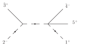
(a) Diagram A

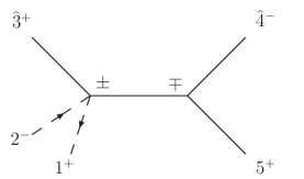
(b) Diagram B

Figure 2: Recursive diagrams contributing to $\bar{q}^{+}(p_{1})q^{-}(p_{2})\to g^{+}(p_{3})g^{-}(p_{4})g^{+}(p_{5})$.

The two diagrams with internal gluons both vanish, due to the vanishing of $M^{+-++}$ and the vanishing of the $(++-)$ gluon vertex with the shifts we have chosen. For the remaining diagram we use

$$M^{+--+}=-[4|1|3\rangle\frac{(13)[42]+[14](32)}{4\ p_{3}\cdot p_{4}\ p_{4}\cdot p_{1}},$$ (4.1)

and strip the fermion $u^{-}(p_{2})$, leaving

$$M^{+\bullet-+}=-[4|1|3\rangle\ \bar{u}^{+}(p_{1})\ \frac{u^{+}(p_{3})\bar{u}^{+}(p_{4})+u^{-}(p_{4})\bar{u}^{-}(p_{3})}{4\ p_{3}\cdot p_{4}\ p_{4}\cdot p_{1}}.$$ (4.2)

After the appropriate relabelling this can be used in Diagram A, which can then be written

$$A = -[5|1|\widehat{4}\rangle\ \bar{u}^{+}(p_{1})\ \frac{u^{+}(\widehat{p_{4}})\bar{u}^{+}(p_{5})+u^{-}(p_{5})\bar{u}^{-}(\widehat{p_{4}})}{4\ p_{5}\cdot\widehat{p_{4}}\ p_{5}\cdot p_{1}}\ \frac{({\raise-1.31944pt\hbox to5.03125pt{\hss/\hss}\hbox to0.0pt{\hss$p$}}_{2}-{\raise 1.11111pt\hbox to5.55557pt{\hss/\hss}\hbox to0.0pt{\hss$\widehat{p}$}}_{3}+m)}{(p_{2}-p_{3})^{2}-m^{2}}$$ (4.3)

$$\times \frac{{\raise-0.34723pt\hbox to4.05904pt{\hss/\hss}\hbox to0.0pt{\hss$\epsilon$}}^{+}(\widehat{p_{3}})}{\sqrt{2}}u^{-}(p_{2}).$$

Due to our choice of marking, all the hats in the numerator can be removed. The shifted part of the propagator is killed by the gluon polarization vector. We are left with

$$M^{+-+-+}=[5|1|4\rangle\left[\frac{m(14)(42)[53]+[15](42)[3|2|4\rangle-(14)[32][5|1|4\rangle}{8\ p_{5}\cdot p_{1}\ p_{2}\cdot p_{3}\ \widehat{p}_{4}\cdot p_{5}\ \langle 43\rangle}\right].$$ (4.4)

We can work out $z$ from the requirement that $\widehat{P}^{2}=(p_{2}-\widehat{p}_{3})^{2}=m^{2}$, and find

$$z=\frac{-2\ p_{2}\cdot p_{3}}{[3|2|4\rangle}.$$ (4.5)

The product $\widehat{p}_{4}\cdot p_{5}$ is then

$$\widehat{p}_{4}\cdot p_{5} = (p_{4}-z\ \eta)\cdot p_{5}$$ (4.6)

$$= p_{4}\cdot p_{5}+\frac{p_{2}\cdot p_{3}}{[3|2|4\rangle}[3|5|4\rangle.$$ (4.7)

The result (4.4) is much more compact than the expression obtained from a Feynman diagram calculation, with which it agrees. See Section 5 for the Feynman results for this process in terms of massive spinor products.

4.1 Results for Helicity Conserving Amplitudes

Here we give all the helicity conserving QCD amplitudes for $\bar{q}q\to ggg$. By helicity conserving we mean those amplitudes where the spin polarizations of the fermions are $+-$, in the sense described in Section 2. Whether these labels actually correspond physically to helicity depends on the choice of $k_{0}$. We choose to mark adjacent gluons, so that each amplitude has contributing recursive diagrams of the form of Fig. 2a and Fig. 2b, that is, we have a diagram with an internal fermion and a diagram with an internal gluon. The vanishing of the $2\to 2$ amplitude $M^{+-++}$ simplifies those cases where there is a majority of positive helicity gluons. In particular, the diagrams with an internal gluon vanish. In the remaining cases, we evaluate such diagrams in the same way as in Ref. [9], using identities such as

$$[A\widehat{P}] = \frac{[A|P|i\rangle}{\langle\widehat{P}i\rangle},$$ (4.8)

$$\langle\widehat{P}B\rangle = \frac{[j|P|B\rangle}{[j\widehat{P}]},$$ (4.9)

with $i$ and $j$ as in (3.1). These identities hold only when the marked particles $i$ and $j$ are massless.

The results presented here are valid for arbitrary spin polarizations. Choosing a polarization basis amounts to choosing the vector $k_{0}$, and when this is done the expressions below will simplify. In the helicity basis for example, in which we choose $k_{0}$ to be parallel to the line of approach of the fermions, the building block $M^{+---}$ vanishes. This causes the first term in each of the mostly-minus amplitudes below to vanish.

$$M^{+-+-+}=[5|1|4\rangle\left[\frac{m(14)(42)[53]+[15](42)[3|2|4\rangle-(14)[32][5|1|4\rangle}{8\ p_{5}\cdot p_{1}\ p_{2}\cdot p_{3}\ \widehat{p}_{4}\cdot p_{5}\ \langle 43\rangle}\right]$$ (4.10)

where $i=3$, $j=4$ and

$$\widehat{p}_{4}\cdot p_{5}=p_{4}\cdot p_{5}+\frac{p_{2}\cdot p_{3}}{[3|2|4\rangle}[3|5|4\rangle.$$

$$\begin{split}&M^{+-++-}=[\widehat{4}|1|5\rangle\times\\ &\left[\frac{m[1\widehat{4}][32]\langle 54\rangle+[1\widehat{4}](42)[3|2|5\rangle+2p_{5}\cdot p_{1}(15)[32]+m(15)(42)[43]}{8\ p_{2}\cdot p_{3}\ \widehat{p}_{4}\cdot p_{5}\ p_{5}\cdot p_{1}\langle 43\rangle}\right]\end{split}$$ (4.11)

where $i=3$, $j=4$ and

$$\widehat{p_{4}}\cdot p_{5}=p_{4}\cdot p_{5}+\frac{p_{2}\cdot p_{3}}{[3|2|4\rangle}[3|5|4\rangle,\hskip 31.29802pt|\widehat{4}]=|4]-\frac{(-2\ p_{2}\cdot p_{3})}{[3|2|4\rangle}|3].$$

$$\begin{split}&M^{+--++}=[\widehat{4}|2|3\rangle\times\\ &\left[\frac{m[\widehat{4}2][15]\langle 43\rangle-[\widehat{4}2](14)[5|1|3\rangle-2p_{2}\cdot p_{3}[15](32)+m(14)(32)[54]}{8\ p_{2}\cdot p_{3}\ p_{3}\cdot\widehat{p}_{4}\ p_{5}\cdot p_{1}\langle 54\rangle}\right]\end{split}$$ (4.12)

where $i=5$, $j=4$ and

$$p_{3}\cdot\widehat{p}_{4}=p_{3}\cdot p_{4}+\frac{p_{1}\cdot p_{5}}{[5|1|4\rangle}[5|3|4\rangle,\hskip 31.29802pt|\widehat{4}]=|4]-\frac{(-2\ p_{1}\cdot p_{5})}{[5|1|4\rangle}|5].$$

$$\begin{split}&M^{+-+--}=\frac{m[21]\langle 45\rangle^{3}}{\langle 34\rangle\big{[}\langle 35\rangle 2p_{5}\cdot p_{1}+\langle 34\rangle[4|2|5\rangle\big{]}(p_{1}+p_{2})^{2}}\ +\\ [3|2|\widehat{4}\rangle&\left[\frac{m(\widehat{4}2)(15)[43]-(\widehat{4}2)[14][3|1|5\rangle-2p_{2}\cdot p_{3}(15)[32]+m[14][32]\langle 54\rangle}{8\ p_{2}\cdot p_{3}\ p_{3}\cdot\widehat{p}_{4}\ p_{5}\cdot p_{1}[54]}\right]\end{split}$$ (4.13)

where $i=4$, $j=5$, and

$$p_{3}\cdot\widehat{p}_{4}=p_{3}\cdot p_{4}+\frac{p_{1}\cdot p_{5}}{[4|1|5\rangle}[4|3|5\rangle,\hskip 31.29802pt(\widehat{4}2)=(42)+\frac{(2p_{1}\cdot p_{5})}{[4|1|5\rangle}(52).$$

$$M^{+--+-} = \frac{m[21]\langle 53\rangle^{4}}{\sqrt{2}\ \langle 43\rangle\langle 45\rangle\big{[}\langle 53\rangle 2\ p_{2}\cdot p_{3}+\langle 54\rangle[4|2|3\rangle\big{]}(p_{1}+p_{2})^{2}}$$

$$+ [4|1|5\rangle\left[\frac{m[14][42]\langle 53\rangle+(15)[42][4|2|3\rangle-[14](32)[4|1|5\rangle}{8\ p_{5}\cdot p_{1}\ p_{2}\cdot p_{3}\ \widehat{p}_{4}\cdot p_{5}[34]}\right]$$

where $i=4$, $j=3$, and

$$\widehat{p}_{4}\cdot p_{5}=p_{4}\cdot p_{5}+\frac{p_{2}\cdot p_{3}}{[4|2|3\rangle}[4|5|3\rangle.$$

$$M^{+---+}=\frac{m[21]\langle 43\rangle^{3}}{\sqrt{2}\ \langle 45\rangle\big{[}\langle 53\rangle 2\ p_{2}\cdot p_{3}+\langle 54\rangle[4|2|3\rangle\big{]}(p_{1}+p_{2})^{2}}\ +$$ (4.15)

$$[5|1|\widehat{4}\rangle\times\left[\frac{m(1\widehat{4})(32)[54]+(1\widehat{4})[42][5|2|3\rangle+2p_{5}\cdot p_{1}[15](32)+m[15][42]\langle 43\rangle}{8\ p_{2}\cdot p_{3}\ \widehat{p}_{4}\cdot p_{5}\ p_{5}\cdot p_{1}[34]}\right]$$

where $i=4$, $j=3$, and

$$\widehat{p}_{4}\cdot p_{5} = p_{4}\cdot p_{5}+\frac{p_{2}\cdot p_{3}}{[4|2|3\rangle}[4|5|3\rangle,\hskip 31.29802pt(1\widehat{4})=(14)+\frac{(2\ p_{2}\cdot p_{3})}{[4|2|3\rangle}(13),$$

$$|\widehat{4}\rangle = |4\rangle+\frac{2\ p_{2}\cdot p_{3}}{[4|2|3\rangle}|3\rangle$$

$$M^{+----}=\frac{m\langle 5\widehat{4}\rangle[4|2|3\rangle[12][45]}{4\ [45]^{2}\ p_{5}\cdot p_{1}\ p_{2}\cdot p_{3}\ [34]}$$ (4.16)

where

$$\langle 5\widehat{4}\rangle=\langle 54\rangle+\frac{2p_{2}\cdot p_{3}}{[4|2|3\rangle}\langle 53\rangle.$$

$$M^{+-+++}=0$$ (4.17)

The amplitudes with fermion helicities $-+$ can be obtained from those above by complex conjugation.

4.2 Results for Helicity Flip Amplitudes

We now consider the helicity flip amplitudes. These have fermion spin polarization labels $\pm\pm$. In this case we are unable to evaluate diagrams with an internal gluon due to products such as $(\widehat{P}k)$ where $k$ is massive. For those amplitudes in which all gluons have the same helicity, the internal gluon diagrams vanish anyway:

$$M^{++---}=m\langle\widehat{4}3\rangle\left[\frac{m(15)(42)[43]+[14](32)[4|1|5\rangle-[14](42)[3|1|5\rangle}{-4\ p_{5}\cdot p_{1}\ p_{2}\cdot p_{3}[34]^{2}[54]}\right]$$ (4.18)

where $i=4$, $j=5$ and

$$|\widehat{4}\rangle=|4\rangle+\frac{2\ p_{5}\cdot p_{1}}{[4|1|5\rangle}|5\rangle.$$

$$M^{+++++}=m[5\widehat{4}]\left[\frac{m(14)(32)\langle 54\rangle+(14)\langle 42\rangle[3|2|5\rangle-(15)\langle 42\rangle[3|2|4\rangle}{-4\ p_{5}\cdot p_{1}\ p_{2}\cdot p_{3}\langle 45\rangle^{2}\langle 43\rangle}\right]$$ (4.19)

where $i=3$, $j=4$ and

$$|\widehat{4}]=|4]+\frac{2\ p_{2}\cdot p_{3}}{[3|2|4\rangle}|3].$$

The amplitudes $M^{--+++}$ and $M^{-----}$ are obtained from those above by complex conjugation. For the remaining amplitudes we resort to Feynman diagrams.

5 Feynman Results

Here we give results for $\bar{q}q\to ggg$ derived from Feynman rules. Note that in a given amplitude all the helicities can be flipped by complex conjugation.

$$M^{+--+-} = -[4|2|3\rangle\left[\frac{m[14][42]\langle 53\rangle+(15)[42][4|2|3\rangle-[14](32)[4|1|5\rangle}{8\ p_{5}\cdot p_{1}\ p_{2}\cdot p_{3}\ p_{3}\cdot p_{4}\ [54]}\right]$$ (5.1)

$$+ \langle 35\rangle\bigg{[}\frac{m[14][42]\langle 53\rangle+(15)[42][4|2|3\rangle-[14](32)[4|1|5\rangle}{8\ p_{2}\cdot p_{3}\ p_{3}\cdot p_{4}\ p_{4}\cdot p_{5}}\bigg{]}$$

$$+ \frac{\langle 35\rangle^{2}}{\langle 34\rangle\langle 45\rangle(p_{1}+p_{2})^{2}}\bigg{[}\frac{[14](32)+(13)[42]}{[54]}+\frac{[14](52)+(15)[42]}{[34]}\bigg{]}.$$

$$M^{+-++-} = -[4|1|5\rangle\left[\frac{-m(15)(52)[43]+(15)[32][4|1|5\rangle-[14](52)[3|2|5\rangle}{8\ p_{5}\cdot p_{1}\ p_{2}\cdot p_{3}\ p_{4}\cdot p_{5}\ \langle 53\rangle}\right]$$ (5.2)

$$+ [43][4|1|5\rangle\bigg{[}\frac{[14](52)+(15)[42]}{4\ p_{5}\cdot p_{1}\ p_{3}\cdot p_{4}\langle 53\rangle[54]}\bigg{]}$$

$$- [43]\bigg{[}\frac{[14](52)[3|1|5\rangle+(15)[32][4|1|5\rangle-m(15)(52)[43]}{4\ p_{5}\cdot p_{1}\ p_{3}\cdot p_{4}\ p_{4}\cdot p_{5}}\bigg{]}$$

$$- \frac{[43]^{2}\langle 35\rangle}{2\ p_{3}\cdot p_{4}[54](p_{1}+p_{2})^{2}}\bigg{[}\frac{[14](52)+(15)[42]}{\langle 53\rangle}+\frac{[13](52)+(15)[32]}{\langle 54\rangle]}\bigg{]}.$$

$$M^{+-+--} = [3|2|4\rangle\left[\frac{m[13][32]\langle 54\rangle-[13](42)[3|1|5\rangle+(15)[32][3|2|4\rangle}{-8\ p_{5}\cdot p_{1}\ p_{2}\cdot p_{3}\ p_{3}\cdot p_{4}\ [53]}\right]$$ (5.3)

$$+ \langle 45\rangle[3|2|4\rangle\bigg{[}\frac{[13](42)+(14)[32]}{4\ p_{2}\cdot p_{3}\ p_{4}\cdot p_{5}\langle 43\rangle[35]}\bigg{]}$$

$$+ \langle 45\rangle\bigg{[}\frac{[13](42)[3|2|5\rangle+(15)[32][3|2|4\rangle+m[13][32]\langle 54\rangle]}{8\ p_{2}\cdot p_{3}\ p_{3}\cdot p_{4}\ p_{4}\cdot p_{5}}\bigg{]}$$

$$+ \frac{\langle 45\rangle^{2}[53]}{2\ p_{4}\cdot p_{5}\langle 43\rangle(p_{1}+p_{2})^{2}}\bigg{[}\frac{[13](52)+(15)[32]}{[43]}+\frac{[13](42)+(14)[32]}{[53]}\bigg{]}.$$

The corresponding helicity flip amplitudes can be obtained from these simply by altering the types of brackets. For example, suppose we wish to extract $M^{---+-}$ from $M^{+--+-}$ given above. We can achieve this by changing brackets as follows:

$$[1k] \to (1k),$$ (5.4)

$$(1k) \to \langle 1k\rangle,$$ (5.5)

where $k$ is massless. Sandwich products such as $[4|1|5\rangle$ are not changed. This transformation results in

$$M^{---+-} = -[4|2|3\rangle\left[\frac{m(14)[42]\langle 53\rangle+\langle 15\rangle[42][4|2|3\rangle-(14)(32)[4|1|5\rangle}{8\ p_{5}\cdot p_{1}\ p_{2}\cdot p_{3}\ p_{3}\cdot p_{4}\ [54]}\right]$$ (5.6)

$$+ \langle 35\rangle\bigg{[}\frac{m(14)[42]\langle 53\rangle+\langle 15\rangle[42][4|2|3\rangle-(14)(32)[4|1|5\rangle}{8\ p_{2}\cdot p_{3}\ p_{3}\cdot p_{4}\ p_{4}\cdot p_{5}}\bigg{]}$$

$$+ \frac{\langle 35\rangle^{2}}{\langle 34\rangle\langle 45\rangle(p_{1}+p_{2})^{2}}\bigg{[}\frac{(14)(32)+\langle 13\rangle[42]}{[54]}+\frac{(14)(52)+\langle 15\rangle[42]}{[34]}\bigg{]}.$$

Other amplitudes can be found by analogous bracket alterations.

6 Summary

We have calculated all the partial spin amplitudes for the $\bar{q}q\to ggg$ scattering process where $q$ is a massive fermion. For most of the partial amplitudes we were able to use the BCFW recursion relations to obtain fairly compact expressions. This was achieved by following the idea of Ref. [27] of stripping lower point amplitudes of their external fermion wavefunctions before inserting them into the recursion. We used a particular representation of massive spinors, along the lines of the appendix of Ref. [28], to define massive spinor products. In this method information regarding the polarization of the fermion spins is contained in the definition of the spinor products, rather than explicitly in the amplitude.

We derived very compact results for the helicity conserving partial amplitudes. This simplicity can be attributed to the vanishing of certain $2\to 2$ scattering amplitudes, which meant that in some cases we were able to avoid diagrams with internal gluons. We were unable to treat the helicity flip amplitudes in the same way (except for the case where all the gluon helicities are the same), since we were unable to evaluate the corresponding recursive diagrams with internal gluons. For these amplitudes we instead provided expressions derived from Feynman diagrams, also in terms of massive spinor products.

These results represent an interesting test of the BCFW recursion relations [9, 10]. The massive spinor products we used are well suited to calculations with massive fermions. Application of these techniques to higher order processes with massive fermions, such as $\bar{q}q\to gggg$, should be possible though would be accompanied by an increase in complexity.

Acknowledgements

KJO acknowledges the award of a PPARC studentship. We are grateful to Valery Khoze for useful discussions.

Appendices

Appendix A Notation and Conventions

We have used products of Dirac spinors

$$[ij]=\bar{u}^{+}(i)u^{-}(j),\hskip 28.45274pt\langle ij\rangle=\bar{u}^{-}(i)u^{+}(j),\hskip 28.45274pt(ij)=\bar{u}^{\pm}(i)u^{\pm}(j)$$ (A.1)

with massive $p_{i}$,$p_{j}$. To evaluate these we use two arbitrary four vectors $k_{0}$ and $k_{1}$, such that

$$k_{0}^{2}=0,\hskip 28.45274ptk_{1}^{2}=-1,\hskip 28.45274ptk_{0}\cdot k_{1}=0.$$ (A.2)

Then

$$[ij] = \frac{(p_{i}\cdot k_{0})(p_{j}\cdot k_{1})-(p_{j}\cdot k_{0})(p_{i}\cdot k_{1})-i\epsilon_{\mu\nu\rho\sigma}k_{0}^{\mu}p_{i}^{\nu}p_{j}^{\rho}k_{1}^{\sigma}}{\sqrt{(p_{i}\cdot k_{0})(p_{j}\cdot k_{0})}}$$ (A.3)

$$\langle ij\rangle = \frac{(p_{j}\cdot k_{0})(p_{i}\cdot k_{1})-(p_{j}\cdot k_{1})(p_{i}\cdot k_{0})-i\epsilon_{\mu\nu\rho\sigma}k_{0}^{\mu}p_{i}^{\nu}p_{j}^{\rho}k_{1}^{\sigma}}{\sqrt{(p_{i}\cdot k_{0})(p_{j}\cdot k_{0})}}$$ (A.4)

$$(ij) = m_{i}\left(\frac{p_{j}\cdot k_{0}}{p_{i}\cdot k_{0}}\right)^{\frac{1}{2}}+i\leftrightarrow j$$ (A.5)

where $m_{i}$ is negative if $i$ is an antiparticle. Different choices of $k_{0}$ correspond to different choices of the quantization axis of a massive fermion’s spin, as described in Section 2.

We use the notation

$$\bar{u}^{+}(i)\ {\raise-1.31944pt\hbox to5.03125pt{\hss/\hss}\hbox to0.0pt{\hss$p$}}\ u^{+}(j) = [i|p|j\rangle=[ip]\langle pj\rangle+(ip)(pj),$$ (A.6)

$$\bar{u}^{-}(i)\ {\raise-1.31944pt\hbox to5.03125pt{\hss/\hss}\hbox to0.0pt{\hss$p$}}\ u^{-}(j) = \langle i|p|j]=\langle ip\rangle[pj]+(ip)(pj).$$ (A.7)

Whereas for massless vectors $k_{i}$,$k_{j}$ we have the familiar relation $2k_{i}\cdot k_{j}=\langle ij\rangle[ji]$, in the massive case this is extended to

$$2p_{i}\cdot p_{j}=\langle ij\rangle[ji]+(ij)^{2}.$$ (A.8)

For any massive $i$,$j$ and massless $k,l$ we have

$$(ik)(jl) = (il)(jk),$$ (A.9)

$$(ik)[li]+[ik](li) = m_{i}[lk],$$ (A.10)

$$\bar{u}^{\pm}(p_{k})\ {\raise-1.31944pt\hbox to6.96053pt{\hss/\hss}\hbox to0.0pt{\hss$p_{i}$}}\ u^{\mp}(p_{l}) = 0$$ (A.11)

The Schouten identity holds,

$$\langle a\ b\rangle\langle c\ d\rangle+\langle a\ c\rangle\langle d\ b\rangle+\langle a\ d\rangle\langle b\ c\rangle=0.$$ (A.12)

For gluon polarization vectors we use

$$\epsilon^{+}_{\mu}(p,k) = \frac{\bar{u}^{-}(k)\ \gamma_{\mu}\ u^{-}(p)}{\sqrt{2}\ \langle kp\rangle},$$ (A.13)

$$\epsilon^{-}_{\mu}(p,k) = \frac{\bar{u}^{+}(k)\ \gamma_{\mu}\ u^{+}(p)}{\sqrt{2}\ [pk]},$$ (A.14)

which take the slashed form

$${\raise-0.34723pt\hbox to4.05904pt{\hss/\hss}\hbox to0.0pt{\hss$\epsilon$}}^{+}(p,k) = \sqrt{2}\ \frac{u_{+}(k)\bar{u}_{+}(p)+u_{-}(p)\bar{u}_{-}(k)}{\langle kp\rangle},$$ (A.15)

$${\raise-0.34723pt\hbox to4.05904pt{\hss/\hss}\hbox to0.0pt{\hss$\epsilon$}}^{-}(p,k) = \sqrt{2}\ \frac{u_{+}(p)\bar{u}_{+}(k)+u_{-}(k)\bar{u}_{-}(p)}{[pk]}.$$ (A.16)

We use a shorthand form for the amplitude in which we display only the helicities of the particles involved. So for example,

$$M(\bar{q}^{+}_{1},q^{-}_{2}\ ;\ 3^{+},4^{-},5^{+})\sim M^{(+-+-+)}.$$ (A.17)

Appendix B Colour Decomposition

The calculation of multi-parton scattering amplitudes in perturbative QCD becomes problematic very quickly as the number of partons increases, due to the sheer number of diagrams and the complicated gluon self-interactions. One technique to circumvent this is to split the set of all Feynman diagrams contributing to a particular amplitude into gauge invariant subsets. Then different gauges can be used in the evaluation of each subset. This simplifies the overall calculation considerably. Each subset of Feynman diagrams is called a partial amplitude. We use the normalization

$$\mbox{Tr}(T^{A}T^{B})=\delta_{ab}.$$ (B.1)

where the $T^{i}$ are matrices of the fundamental representation of $SU(3)$. This convention leads to colour-ordered Feynman rules as given in [31]. The colour decomposition for processes with a pair of quarks is then

$$A(\bar{q},q\ ;\ g_{1},g_{2}\cdots g_{n})=\sum_{\sigma}\big{(}T^{a_{\sigma(1)}}\dots T^{a_{\sigma(n)}}\big{)}_{ij}M(\bar{q},q\ ;\ g_{\sigma(1)},g_{\sigma(2)}\cdots g_{\sigma(n)}).$$ (B.2)

Here $\sigma$ is the set of all distinct cyclic orderings of the gluons. The colour information in a given amplitude is contained purely in the group theoretical prefactors, while all the kinematical information is contained in the partial amplitudes $M(\sigma)$. It is useful to note that amplitudes in QED can be obtained from amplitudes in QCD by replacing all the colour matrices $T^{A}$ with the identity matrix. For references and a more detailed description of colour decomposition, the reader is directed to Ref. [31].

References

• [1] E. Witten, “Perturbative gauge theory as a string theory in twistor space”, Commun. Math. Phys.  252 (2004) 189 [arXiv:hep-th/0312171].
• [2] F. Cachazo, P. Svrcek and E. Witten, “MHV vertices and tree amplitudes in gauge theory”, JHEP 0409 (2004) 006 [arXiv:hep-th/0403047].
• [3] G. Georgiou and V. V. Khoze, “Tree amplitudes in gauge theory as scalar MHV diagrams”, JHEP 0405 (2004) 070 [arXiv:hep-th/0404072].
• [4] G. Georgiou, E. W. N. Glover and V. V. Khoze, “Non-MHV tree amplitudes in gauge theory”, JHEP 0407 (2004) 048 [arXiv:hep-th/0407027].
• [5] N. E. J. Bjerrum-Bohr, D. C. Dunbar, H. Ita, W. B. Perkins and K. Risager, “MHV-vertices for gravity amplitudes”, JHEP 0601 (2006) 009 [arXiv:hep-th/0509016].
• [6] T. G. Birthwright, E. W. N. Glover, V. V. Khoze and P. Marquard, “Collinear limits in QCD from MHV rules”, JHEP 0507 (2005) 068 [arXiv:hep-ph/0505219].
• [7] L. J. Dixon, E. W. N. Glover and V. V. Khoze, “MHV rules for Higgs plus multi-gluon amplitudes”, JHEP 0412 (2004) 015 [arXiv:hep-th/0411092].
• [8] A. Brandhuber, B. Spence and G. Travaglini, “From trees to loops and back”, JHEP 0601 (2006) 142 [arXiv:hep-th/0510253].
• [9] R. Britto, F. Cachazo and B. Feng, “New recursion relations for tree amplitudes of gluons”, Nucl. Phys. B 715 (2005) 499 [arXiv:hep-th/0412308].
• [10] R. Britto, F. Cachazo, B. Feng and E. Witten, “Direct proof of tree-level recursion relation in Yang-Mills theory”, Phys. Rev. Lett.  94 (2005) 181602 [arXiv:hep-th/0501052].
• [11] M. x. Luo and C. k. Wen, “Recursion relations for tree amplitudes in super gauge theories”, JHEP 0503 (2005) 004 [arXiv:hep-th/0501121].
• [12] K. J. Ozeren and W. J. Stirling, “MHV techniques for QED processes”, JHEP 0511 (2005) 016 [arXiv:hep-th/0509063].
• [13] J. Bedford, A. Brandhuber, B. J. Spence and G. Travaglini, “A recursion relation for gravity amplitudes”, Nucl. Phys. B 721 (2005) 98 [arXiv:hep-th/0502146].
• [14] Z. Bern, L. J. Dixon and D. A. Kosower, “Bootstrapping multi-parton loop amplitudes in QCD”, arXiv:hep-ph/0507005.
• [15] Z. Bern, L. J. Dixon and D. A. Kosower, “The last of the finite loop amplitudes in QCD”, Phys. Rev. D 72 (2005) 125003 [arXiv:hep-ph/0505055].
• [16] Z. Bern, L. J. Dixon and D. A. Kosower, “On-shell recurrence relations for one-loop QCD amplitudes”, Phys. Rev. D 71 (2005) 105013 [arXiv:hep-th/0501240].
• [17] Z. Bern, N. E. J. Bjerrum-Bohr, D. C. Dunbar and H. Ita, “Recursive calculation of one-loop QCD integral coefficients”, JHEP 0511 (2005) 027 [arXiv:hep-ph/0507019].
• [18] C. Schwinn and S. Weinzierl, “SUSY Ward identities for multi-gluon helicity amplitudes with massive quarks”, arXiv:hep-th/0602012.
• [19] M. T. Grisaru, H. N. Pendleton and P. van Nieuwenhuizen, “Supergravity And The S Matrix”, Phys. Rev. D 15 (1977) 996.
M. T. Grisaru and H. N. Pendleton, “Some Properties Of Scattering Amplitudes In Supersymmetric Theories”, Nucl. Phys. B 124 (1977) 81.
• [20] P. Ferrario, G. Rodrigo and P. Talavera, “Compact multigluonic scattering amplitudes with heavy scalars and fermions”, arXiv:hep-th/0602043.
• [21] D. Forde and D. A. Kosower, “All-multiplicity amplitudes with massive scalars”, arXiv:hep-th/0507292.
• [22] F. A. Berends and W. T. Giele, “Recursive Calculations For Processes With N Gluons”, Nucl. Phys. B 306 (1988) 759.
• [23] G. Rodrigo, “Multigluonic scattering amplitudes of heavy quarks”, JHEP 0509 (2005) 079 [arXiv:hep-ph/0508138].
• [24] Z. Bern, L. J. Dixon, D. C. Dunbar and D. A. Kosower, “One loop n point gauge theory amplitudes, unitarity and collinear limits”, Nucl. Phys. B 425 (1994) 217 [arXiv:hep-ph/9403226].
Z. Bern, L. J. Dixon, D. C. Dunbar and D. A. Kosower, “Fusing gauge theory tree amplitudes into loop amplitudes”, Nucl. Phys. B 435 (1995) 59 [arXiv:hep-ph/9409265].
• [25] C. Quigley and M. Rozali, “Recursion relations, helicity amplitudes and dimensional regularization”, arXiv:hep-ph/0510148
• [26] S. D. Badger, E. W. N. Glover, V. V. Khoze and P. Svrcek, “Recursion relations for gauge theory amplitudes with massive particles”, JHEP 0507 (2005) 025 [arXiv:hep-th/0504159].
• [27] S. D. Badger, E. W. N. Glover and V. V. Khoze, “Recursion relations for gauge theory amplitudes with massive vector bosons and fermions”, JHEP 0601 (2006) 066 [arXiv:hep-th/0507161].
• [28] R. Kleiss and W. J. Stirling, “Cross-Sections For The Production Of An Arbitrary Number Of Photons In Electron - Positron Annihilation”, Phys. Lett. B 179 (1986) 159.
• [29] R. K. Ellis, W. J. Stirling and B. R. Webber, Camb. Monogr. Part. Phys. Nucl. Phys. Cosmol.  8 (1996) 1.
• [30] K. Risager, “A direct proof of the CSW rules”, JHEP 0512 (2005) 003 [arXiv:hep-th/0508206].
• [31] L. J. Dixon, “Calculating scattering amplitudes efficiently”, arXiv:hep-ph/9601359.