A Consistent Prescription for the Production Involving Massive Quarks in Hadron Collisions

Abstract:

This paper addresses the issue of production of charm or bottom quarks in association with a high $p_{T}$ process in hadron hadron collision. These quarks can be produced either as part of the hard scattering process or as a remnant from the structure functions. The latter sums terms of the type $(\alpha_{s}log(p_{T}/m_{q}))^{n}$. If structure functions of charm or bottom quarks are used together with a hard process which also allows production of these quarks double counting occurs. This paper describes the correct procedure and provides two examples of its implimentation in single top and Drell-Yan at the LHC.

1 Introduction

The production of states by a hard scattering QCD process in hadron collision is described by the parton model which separates it into perturbative (calculable) process and a soft non-perturbative piece. Consider the production of a top quark pair via the partonic process $gg\to t\overline{t}$. There are many gluons present in the process but the only top quarks arise from the hard scatter itself. Top quarks can also be produced singly via the process $gb\to W^{-}t$. In order for this to occur the incoming bottom quark is viewed as a constituent (parton) of the incoming hadron. Alternatively one could begin with a two gluon initial state and consider the hard process as $gg\to t\overline{b}W^{-}$. These two processes cannot be added as the QCD approximation that produces the $b$ parton in the first case is partially accounted for by the latter process. A careful separation of “hard” and “soft” components is needed so that a consistent result can be obtained. The rest of this paper demonstrates such a separation. The rest of this section is concerned with introducing the formalism. Section 2 shows explicitly how to relate processes with one more (or less) parton in the hard scattering. Section 3 presents some explicit examples of the Monte-Carlo implementation of this formalism. Finally some conclusions are drawn.

The QCD-based parton model is based on the factorization theorems [1, 2, 3, 4, 5] according to which the squared amplitude for a process $\rm A,B\to X$ can be decomposed into a “hard” and “soft” (or alternatively denoted “short” and “long distance”) parts:

$$|\mathcal{M}_{AB\to X}|^{2} = \sum_{a,b}f_{a/A}\otimes H_{ab\to X}\otimes f_{b/B}$$ (1)

$$= \sum_{a,b}\int\frac{d\xi_{a}}{\xi_{a}}\int\frac{d\xi_{b}}{\xi_{b}}f_{a/A}(\xi_{a},\mu_{F})\,f_{b/B}(\xi_{b},\mu_{F})\,H_{ab\to X}(\xi_{a},\xi_{b},\mu_{F}\ldots),$$

with $\rm a,b$ labeling the incoming partons which have to be summed over and $\rm H(ab\to X)$ denoting the hard (’short time’) part of the squared amplitude. The soft contributions are absorbed into the parton distribution functions $\rm f_{i/I}(\xi_{i},\mu_{F})$ with $\rm\mu_{F}$ being the (factorization) scale at which the two parts were separated. More explicitly, the above theorem states that the collinear (mass) singularities have to be isolated/subtracted from the hard process amplitudes and reabsorbed into the parton distribution functions [3, 4, 5, 6, 7]; all other singularities (UV, soft IR) appearing in the perturbative calculation of the hard process either cancel or are handled by renormalization procedures. It has to be stressed at this point that the renormalization/regularization scheme used in subtracting the UV singularities in turn dictates the precise form of the evolution (DGLAP) equations of the parton distribution functions [1, 3]

$$\frac{d}{d\ln\mu_{F}^{2}}f_{i/I}(z,\mu_{F})=\frac{\alpha_{s}(\mu_{F})}{2\pi}\sum_{j}\int\limits_{z}^{1}\frac{d\xi}{\xi}P_{j\to i}(\frac{z}{\xi},\alpha_{s}(\mu_{F}))\,f_{j/I}(\xi,\mu_{F}),$$ (2)

where $\rm P_{j\to i}$ denote the usual DGLAP evolution kernels and $\rm I$ describes either a parton or a hadron.

An elegant way of isolating the mass singularities in perturbative calculations is found by observing that the pQCD squared amplitude $\rm|\mathcal{M}_{ab\to X}|^{2}$ involving initial state partons $\rm a,b$ is subject to the same factorization theorem:

$$|\mathcal{M}_{ab\to X}|^{2}=\sum_{c,d}f_{c/a}\otimes H_{cd\to X}\otimes f_{d/b},$$ (3)

with the $\rm f_{i/j}$ representing the distribution function of the parton $\rm i$ inside the parton $\rm j$. The above equation holds to any order in perturbation theory. Consequently, since the $|\mathcal{M}_{ab\to X}|^{2}$ can be calculated to any order by using the Feynman rules and the prescriptions for calculating the $\rm f_{i/j}$ to high orders in $\alpha_{s}$ are also well established [1, 21, 22] one can use the procedure of [5, 6, 7] to extract the $H_{cd\to X}$ to the chosen order.

At zero-th order in $\alpha_{s}$:

$$f_{i/j}^{(0)}(\xi)=\delta_{j}^{i}\delta(\xi-1)$$ (4)

and hence:

$$|\mathcal{M}_{ab\to X}^{(0)}|^{2}=H_{ab\to X}^{(0)}.$$ (5)

Subsequently, at first order in $\alpha_{s}$:

$$f_{i/j}(\xi)=f_{i/j}^{(0)}(\xi)+f_{i/j}^{(1)}(\xi),$$ (6)

and thus at this order:

$$|\mathcal{M}_{ab\to X}^{(1)}|^{2}=H_{ab\to X}^{(1)}+\sum_{c}f_{c/a}^{(1)}\otimes H_{cb\to X}^{(0)}+\sum_{d}H_{ad\to X}^{(0)}\otimes f_{d/b}^{(1)},$$ (7)

where formally the virtuality $\rm\mu^{2}$ of the particles $c$ or $d$ (which is in turn proportional to the $(p_{T})^{2}$ of the particles $\bar{c}$ or $\bar{d}$, see Fig. 1) is used as the factorization measure with the limit $\rm\mu_{F}^{2}$: The hard part $\rm H_{ab\to X}^{(1)}$ includes the cases $\rm\mu^{2}\geq\mu_{F}^{2}$ and the soft one the cases $\rm\mu^{2}\leq\mu_{F}^{2}$. Note that in the above equation, the phase space integration over $\bar{c}/\bar{d}$ particles has already been performed (resulting in the convolution integral) and thus the phase space for the final state particles for the soft part formally involves one less particle.

$+$

$+$

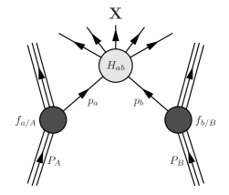
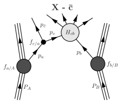
Figure 1: The diagrammatic representation of the method applied in isolating the soft (collinear) terms in propagators corresponding to virtual particles $\rm p_{c}$ and/or $\rm p_{d}$ when calculating the $|\mathcal{M}_{ab\to X}^{(1)}|^{2}$. Note that in factorization theorem the particles incoming into the hard part of the probability amplitude are considered to be on-shell.

The above equation can be inverted to give:

$$H_{ab\to X}^{(1)}=|\mathcal{M}_{ab\to X}^{(1)}|^{2}-\sum_{c}f_{c/a}^{(1)}\otimes|\mathcal{M}_{cb\to X}^{(0)}|^{2}-\sum_{d}|\mathcal{M}_{ad\to X}^{(0)}|^{2}\otimes f_{d/b}^{(1)}$$ (8)

This can be extended to higher orders in perturbation theory. It should be emphasized that the presence of the subtraction terms in the above Eq. 8 prevents double counting when performing the perturbative cross-section calculation since the collinear effects present in the $\rm|\mathcal{M}_{ab\to X}^{(1)}|^{2}$ are removed and re-summed in the parton distribution functions $\rm f_{a/A}$ of the initial hadrons.

After the perturbative expansion of $H_{ab\to X}=H_{ab\to X}^{(0)}+H_{ab\to X}^{(1)}$, given by Eq. 5 and Eq. 8, is inserted into the cross-section expression (Eq. 1) one thus obtains the formula:

$$|\mathcal{M}_{AB\to X}|^{2}=|\mathcal{M}_{AB\to X}^{(0)}|^{2}+|\mathcal{M}_{AB\to X}^{(1)}|^{2}-|\mathcal{M}_{AB\to X}|^{2}_{\mathrm{s}},$$ (9)

with the subtraction terms given by:

$$|\mathcal{M}_{AB\to X}|^{2}_{\mathrm{s}}=\sum_{a,b}f_{a/A}\otimes\sum_{c}f_{c/a}^{(1)}\otimes H_{cb\to X}^{(0)}\otimes f_{b/B}+\sum_{a,b}f_{a/A}\otimes\sum_{d}H_{ad\to X}^{(0)}\otimes f_{d/b}^{(1)}\otimes f_{b/B}.$$ (10)

For further discussion on the ’double counting’ issues it is illuminating to calculate the $f_{i/j}$ at scale $\mu_{F}$ up to the order of $\alpha_{s}$. One starts by writing down the perturbative expansion of the evolution kernels in the DGLAP equations:

$$P_{j\to i}(\xi,\alpha_{s}(\mu_{F}))\,=P_{j\to i}^{(0)}(\xi)+\left(\frac{\alpha_{s}(\mu_{F})}{2\pi}\right)P_{j\to i}^{(1)}(\xi)+\ldots$$ (11)

and observing that the evolution increases the order of $\rm f_{i/j}^{(n)}$ by one. This can explicitly be seen by inserting the zero-th order $\rm f_{i/j}^{(0)}$ of Eq. 4 into the Eq. 2, and increasing the factorization scale from the lowest kinematic limit (mass $\rm m$ of the particle $\rm i$) to the scale $\mu_{F}$, i.e. integrating over the range $\rm[m^{2},\mu_{F}^{2}]$ and keeping only the terms up to the order of $\alpha_{s}$:

$$f_{i/j}(\xi,\mu_{F})=f_{i/j}^{(0)}(\xi)+\frac{\alpha_{s}(\mu_{F})}{2\pi}P_{j\to i}^{(0)}(\xi)\ln\left(\frac{\mu_{F}^{2}}{m^{2}}\right).$$ (12)

The above expression matches the perturbative expansion given by Eq. 6 with the second term identified as the $\rm f_{i/j}^{(1)}$ parton distribution function.

While the expression of Eq. 9 can subsequently be used for estimating the total cross-section of a given process one should take further steps when dealing with the estimation of the differential cross-sections or (equivalently) Monte-Carlo simulation. In a Monte-Carlo simulation the DGLAP parton evolution, re-summed in the parton density functions $f_{i/I}$ (c.f. Eq. 2), is made explicit by evolving the factorization scale from its initial value $\rm\mu_{0}$ to the lowest kinematic limit (or an imposed cutoff). Identifying the evolving factorization scale with the virtuality $\rm\mu^{2}$ of the incoming particle $\rm c$ the probability that the particle $\rm c$ will be un-resolved into a particle $\rm a$ (or equivalently, that a particle $\rm a$ will branch and produce the particle $\rm c$ and an additional spectator particle) is given by the Sudakov term (see e.g. [15]):

$$S_{a}=\exp{\left\{-\int\limits_{\mu^{2}}^{\mu_{0}^{2}}\frac{d\mu^{\prime 2}}{\mu^{\prime 2}}\frac{\alpha_{s}(\mu^{\prime 2})}{2\pi}\times\sum\limits_{c}\int\limits_{\xi_{c}}^{1}\frac{dz}{z}P_{a\to c}(z)\frac{f_{a/I}(\frac{\xi_{c}}{z},\mu^{\prime 2})}{f_{c/I}(\xi_{c},\mu^{\prime 2})}\right\}}.$$ (13)

At each evolution step (branching) the number of particles is increased by one and its contribution to the differential cross-section in terms of $\alpha_{s}$ is also increased by one. The described procedure is commonly known as (initial state) parton showering.

The (next-to-leading order) subtraction terms of Equation 10 thus compensate for the first branching in the backward evolution of the incoming partons participating in the (leading order) term $H_{ab\to X}^{(0)}$. Note that in order to match the subtraction terms in Eq. 8 with the first–order matrix element, the fraction $\rm\xi_{c}$ (or equivalently $\rm\xi_{d}$) of the evolved parton is kept constant and the virtuality is decreased corresponding to a ’backward’ evolution in time from the starting point of virtuality $\rm\mu^{2}_{0}$ of $\rm H_{ab\to X}^{(0)}$. to the virtuality $\rm\mu^{2}$ of $\rm H_{ab\to X}^{(1)}$ (c.f. Figure 1). Writing the expressions of Equation 10 in differential form in $\rm\mu^{2}$ one thus gets for the first term:

$$|\mathcal{M}_{AB\to X}|^{2}_{\mathrm{s}}=\frac{d\mu^{2}}{\mu^{2}}\sum_{a,b,c}\int\frac{d\xi_{a}}{\xi_{a}}\int\frac{d\xi_{b}}{\xi_{b}}\int\frac{d\xi_{c}}{\xi_{c}} \Biggl{\{}f_{a/A}(\xi_{a},\mu_{0}^{2})\,\frac{\alpha_{s}(\mu^{2}_{0})}{2\pi}P_{a\to c}^{(0)}\left(\frac{\xi_{c}}{\xi_{a}}\right)\,$$ (14)

$$H_{cb\to X}^{(0)}(\xi_{c},\xi_{b})\,f_{b/B}(\xi_{b},\mu_{0}^{2})+\ldots\Biggr{\}}$$

and an equivalent expression can be obtained for the second term of Eq. 10. Using again the Eq. 5, multiplying by the flux factor ${1}/{2\sqrt{\lambda(s,m_{A}^{2},m_{B}^{2})}}$, given by the Lorentz invariant function:

$$\lambda(s,m_{1}^{2},m_{2}^{2})=(s-(m_{1}+m_{2})^{2})(s-(m_{1}-m_{2})^{2})$$ (15)

and integrating over the final state n-particle phase space denoted by $\rm\int d\Phi_{X}$, one obtains the first subtraction term:

$$\frac{d\sigma^{(0)}_{s1}(AB\to X)}{d\xi_{a}d\xi_{b}d\mu^{2}d\xi_{c}d\phi}=$$

$$\sum\limits_{a,b,c}\frac{\theta(\mu_{0}^{2}-\mu^{2})}{2\sqrt{\lambda(s,m_{A}^{2},m_{B}^{2})}\xi_{c}\xi_{b}}\frac{\alpha_{s}(\mu^{2}_{0})}{4\pi^{2}\,\mu^{2}}\frac{1}{\xi_{a}}f_{a/A}(\xi_{a},\mu_{0}^{2})\,P_{a\to c}^{(0)}\left(\frac{\xi_{c}}{\xi_{a}}\right)\,f_{b/B}(\xi_{b},\mu_{0}^{2})\times$$

$$\qquad\times\int|\mathcal{M}_{cb\to X}^{(0)}|^{2}(\xi_{c},\xi_{b})d\Phi_{X-\bar{c}}$$ (16)

and equivalently also the second subtraction term by appropriate replacements $a\to b$ and $c\to d$. The two derived equations correspond to the expressions obtained by Chen,Collins et al. [9, 10, 11, 12], derived by the Sudakov exponent expansion.

In addition to writing the cross-sections in differential form, the integration over an angle $\rm\phi$ was introduced, where the angle $\phi$ represents the azimuthal angle of the spectator particle $\rm\bar{c}$ or $\rm\bar{d}$ and is in effect a dummy quantity which nevertheless has to be sampled in a Monte–Carlo simulation procedure. The notation $\rm d\Phi_{X-\bar{c}}$ denotes that the final space integral does not contain the spectator particles $\rm\bar{c}$ or $\rm\bar{d}$ since they are already accounted for in the $\rm(d\xi/\xi)d\mu^{2}d\phi$ differential (see e.g. [1]). In contrast the first order matrix element of Equation 8 is integrated over the full phase space X:

$$\frac{d\sigma^{(1)}(AB\to X)}{dx_{a}dx_{b}}=$$

$$\sum\limits_{a,b}\frac{1}{2\sqrt{\lambda(s,m_{A}^{2},m_{B}^{2})}x_{a}x_{b}}f_{a/A}(x_{a},\mu_{0}^{2})\,f_{b/B}(x_{b},\mu_{0}^{2})\int|\mathcal{M}_{ab\to X}^{(1)}|^{2}(x_{a},x_{b})d\Phi_{X}~{},$$ (17)

whereby the outstanding issue is the kinematic translation between $\rm n-1$ ($\rm X-\bar{c}$) and $\rm n$ ($\rm X$) particle kinematics. Furthermore, one cannot simply equate the variables $\rm\xi_{a,b}$ and $\rm x_{a,b}$, since e.g. in Eq. 1 the $\rm\xi_{c,b}$ terms imply that the incoming particles $\rm c$ and $\rm b$ are on shell in the matrix element calculation while in Eq. 1 in contrast the particle $\rm a$ (as the ’parent’ of particle $\rm c$) is the on-shell one.

The mapping of the kinematic quantities between between the expressions of order $\rm\alpha_{S}$ (i.e. the pQCD derived expression of Eq. 1 and the (showering) subtraction terms of Eq. 1 ) needs a consistent and possibly a formally correct definition. In order to achieve this the prescription developed by Collins et al. of how to merge non-perturbative (parton-shower) calculations with the leading order perturbative pQCD calculations on the level of Monte-Carlo simulations [9, 10, 11, 12] was implemented, which has been explicitly shown to reproduce the NLO $\rm\bar{MS}$ result for a set of processes.

Another outstanding issue is that in case of heavy quarks participating as the initial state partons the (commonly used) approximation of treating the incoming particles as massless can lead to a significant error. This fact, as well as the the solution in terms of consistent treatment of the kinematics in terms of light-cone variables, has been demonstrated in the ACOT prescriptons of how to consistently introduce the factorization in case of non-negligible masses of the colliding partons (e.g. heavy quarks)[6, 7]. The ACOT prescription has in this paper been introduced in the formalism of Monte-Carlo simulation by modifying the prescription of Collins et al. accordingly.

In the Monte–Carlo generation steps one thus has to produce two classes of events; one class is derived from the leading order process with one branching produced by Sudakov parton showering and the second class are events produced from the next-to-leading order hard process calculation (i.e. the pQCD calculation with the appropriate subtraction terms).

2 Kinematic Issues

2.1 Phase-Space Transformation

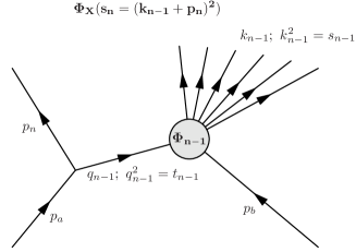
Figure 2: The diagrammatic representation of the method applied in translating a t-channel (space-like) split going from $n$ to $n-1$ particle phase space.

The aim of this section is to derive generic expressions that transform the kinematics from the ’hard’ to the ’soft’ (or showering) n-particle system, i.e. split the ’hard’ $\rm n$-particle phase space involving heavy quarks into $\rm n-1$ ’hard’ $\oplus 1$ ’soft’ particle phase space in order to perform appropriate MC simulation (c.f. Figure 2). As already stated the existing prescriptions deal either with massive particles [6, 7] on the level of integrated cross-sections or with explicit Monte-Carlo algorithms involving light ($\sim$ massless) particles (e.g. [25, 15, 11, 13, 14] ) while no generic combination of the two algorithms is available.

In order to accommodate the particle masses it is convenient to work in light-cone coordinates $p^{\mu}=(p^{+},\vec{p}^{T},p^{-})$ where $\rm p^{\pm}=\frac{1}{\sqrt{2}}(p^{0}\pm p^{3})$ and the remaining two coordinates are considered ’transverse’ $\vec{p}^{T}$. The kinematic prescription of relating the hard $\rm n$-particle kinematics to the soft $\rm n-1$ case is as follows:

1. Incoming hadron A is moving in the $\rm z$ direction and hadron B in the $\rm-z$ direction, carrying momenta $\rm P_{A}$ and $\rm P_{B}$ with the center-of-mass energy $\rm\sqrt{s}$, whereby one can neglect the hadron masses at LHC energies.

2. The incoming partons with momenta $\rm p_{a}$ and $\rm p_{b}$ have the momentum fractions $\rm p_{a}^{+}=x_{a}P_{A}^{+}$ and $\rm p_{b}^{-}=x_{b}P_{B}^{-}$ relative to the parent hadrons and the center-of-mass energy $\sqrt{s_{n}}$.

3. The split propagator (i.e. particle $\rm c$) virtuality $p_{c}^{2}=(p_{a}-p_{\bar{c}})^{2}=t_{n-1}$ (c.f. Fig. 2) gives the $\rm\mu^{2}$ value from $t_{n-1}-m_{\bar{c}}^{2}=-\mu^{2}$. (c.f. Eq. 1).

4. The scale correspondence is given by $\rm s_{n-1}=\mu_{0}^{2}$ (c.f. Eq. 1).

5. All incoming and outgoing particles (partons) are on mass shell.

6. The splitting parameter of the evolution kernel is $\rm z=\frac{\xi_{c}}{\xi_{a}}$ (already used in Eq. 1).

7. The rapidity $\rm y=\frac{1}{2}\ln\left(\frac{k_{n-1}^{+}}{k_{n-1}^{-}}\right)$ of the subsystem (c.f. Figure 2) is preserved in the translation.

In order to further relate the $\rm n$ and $\rm n-1$ particle phase space for hard and soft interpretation one can use the recursive t-channel splitting relation [16, 18]:

$$\Phi_{n}(s_{n},m_{1},m_{2},\ldots,m_{n})=$$

$$=\int\limits_{(\sum_{i=1}^{n-1}m_{i})^{2}}^{(\sqrt{s_{n}}-m_{n})^{2}}\frac{ds_{n-1}}{4\sqrt{\lambda(s_{n},m_{a}^{2},m_{b}^{2})}}\int\limits_{0}^{2\pi}d\varphi_{n}^{*}\int\limits_{t_{n-1}^{-}}^{t_{n-1}^{+}}dt_{n-1}\>\Phi_{n-1}(s_{n-1},m_{1},m_{2},\ldots,m_{n-1}),$$ (18)

where $\rm\varphi_{n}^{*}\equiv\phi$ of Eq. 1 and the limits $t_{n-1}^{\pm}$ are given by analytic, albeit complex expressions [16, 18]. Using the above relation one can introduce the $\rm X-\bar{c}$ particle phase space split into Equation 1 by identifying $\rm p_{\bar{c}}\equiv p_{n}$ :

$$\frac{d\sigma^{(1)}(AB\to X)}{dx_{a}dx_{b}dt_{n-1}ds_{n-1}d\varphi^{*}}=$$

$$\sum\limits_{a,b}\frac{1}{2\sqrt{\lambda(s,m_{A}^{2},m_{B}^{2})}x_{a}x_{b}}f_{a/A}(x_{a},s_{n-1})\,f_{b/B}(x_{b},s_{n-1})\times$$

$$\qquad\times\int|\mathcal{M}_{ab\to X}^{(1)}|^{2}(x_{a},x_{b})\frac{1}{4\sqrt{\lambda(s_{n},m_{a}^{2},m_{b}^{2})}}d\Phi_{X-\bar{c}}~{},$$ (19)

Using the translation prescriptions introduced above, the remaining issue is the relation of the variables $\rm\xi_{a},\xi_{c},\xi_{b}$ with the variables $x_{a},x_{b},s_{n-1}$. The requirement (2) in the list above ensures $\rm\xi_{a}\equiv x_{a}$ since both particles in question are incoming partons originating in hadron A. The remaining relations between $\rm\xi_{c},\xi_{b}$ and $x_{b},s_{n-1}$ are then given by energy and rapidity conservation requirements. The derived relations are explicitly listed in Appendix A.

Combining all the derived rules for kinematic translation one finally obtains a transformation of Eq. 1:

$$\frac{d\sigma^{(0)}_{s1}(AB\to X)}{dx_{a}dx_{b}dt_{n-1}ds_{n-1}d\varphi^{*}}=$$

$$=\mathcal{J}\frac{(\xi_{c},\xi_{b})}{(s_{n-1},x_{b})}\left.\frac{d\sigma^{(0)}_{s1}(AB\to X)}{d\xi_{a}d\xi_{b}d\mu^{2}d\xi_{c}d\phi}\right|_{\xi_{a}\to x_{a},\,\mu^{2}\to-(t_{n-1}-m_{\bar{c}}^{2}),\,\phi\to\varphi^{*},\,(\xi_{c},\xi_{b})\to(s_{n-1},x_{b})},$$ (20)

where $\mathcal{J}\frac{(\bar{\tau},\bar{y})}{(s_{n-1},x_{b})}$ is the Jacobian of the transformation derived in the Appendix A.

An issue which deserves special consideration is the prescribed substitution $t_{n-1}-m_{\bar{c}}^{2}=-\mu^{2}$, where the split particle virtuality $\mu^{2}$ is the propagator virtuality shifted by the spectator mass $m_{\bar{c}}^{2}$. This prescription differs from the one of Collins [9], where the relation is directly $t_{n-1}=-\mu^{2}$ and the spectator (propagator) mass shift is omitted. The reason for this modification is clear when one notes that the phase space limits $[t_{n-1}^{-},t_{n-1}^{+}]$ of the $t_{n-1}$ parameter are functions of $s_{n}$ and invariant masses of the objects (particles) participating in a t-channel split of Equation 2.1 [16, 18] and thus do not match the simple limits $[m_{\bar{c}}^{2},s_{n-1}]$ of the virtuality $\mu^{2}$ in the equation 1. Indeed, studies have shown that the presence of the cutoff $\theta(s_{n-1}+t_{n-1})$ does not provide a sufficient solution since it only sets the upper integration limit to $t_{n-1}^{+}\to-s_{n-1}$ while the lower limit $t_{n-1}^{-}$ can in certain instances be even smaller than $m_{\bar{c}}^{2}$. The reproduction of a logarithmic term of the collinear singularity $\ln\left(\frac{\mu_{F}^{2}}{m^{2}}\right)$ (Eq. 12) with $\mu_{F}^{2}=\mu_{0}^{2}=s_{n-1}$:

$$\int\limits_{t_{n-1}^{-}}^{t_{n-1}^{+}}\frac{\theta(s_{n-1}+t_{n-1})}{t_{n-1}}dt_{n-1}\>=\ln\left(\frac{-s_{n-1}}{t_{n-1}^{-}}\right)\neq\ln\left(\frac{s_{n-1}}{m_{\bar{c}}^{2}}\right)$$ (21)

is thus not satisfied in when using $t_{n-1}=-\mu^{2}$. In order to resolve this issue one needs to return to the basics of the factorization procedure, where the actual collinear singularity (i.e.   the corresponding logarithmic term) is isolated from the (integrated) hard process cross-section (for a nice example with massive particles see e.g. [7]) and these logarithmic terms match with the required collinear logarithm $\ln\left(\frac{\mu_{F}^{2}}{m^{2}}\right)$ only in the high $s_{n}$ (hard center-of-mass) limit. The logarithmic collinear terms can subsequently be traced back to the propagator integral:

$$\int\limits_{t_{n-1}^{-}}^{t_{n-1}^{+}}\frac{dt_{n-1}}{t_{n-1}-m_{\bar{c}}^{2}}=\ln\left(\frac{t_{n-1}^{+}-m_{\bar{c}}^{2}}{t_{n-1}^{-}-m_{\bar{c}}^{2}}\right)~{}~{}~{}\underrightarrow{s_{n}\to\infty}~{}~{}~{}\ln\left(\frac{s_{n-1}}{m_{\bar{c}}^{2}}\right).$$ (22)

The expression of Eq. 22 is indeed found to match the logarithmic terms of [7] exactly. In order to reproduce the collinear cutoff one thus has to put $-\mu^{2}=t_{n-1}-m_{\bar{c}}^{2}$ which, combined with the factorization cutoff $\theta(\mu_{F}^{2}-\mu^{2})=\theta(s_{n-1}-\mu^{2})$, reproduces the required logarithm in the high $s_{n}$ limit:

$$\int\limits_{-(t_{n-1}^{-}-m_{\bar{c}}^{2})}^{-(t_{n-1}^{+}-m_{\bar{c}}^{2})}\frac{\theta(s_{n-1}-\mu^{2})}{\mu^{2}}d\mu^{2}\>=\ln\left(\frac{s_{n-1}}{-(t_{n-1}^{-}-m_{\bar{c}}^{2})}\right)~{}~{}~{}\underrightarrow{s_{n}\to\infty}~{}~{}~{}\ln\left(\frac{s_{n-1}}{m_{\bar{c}}^{2}}\right).$$ (23)

2.2 Monte-Carlo Generation Steps

Figure 3: The definition of the reference Collins-Soper frame as the rest frame of the subsystem $\rm s_{n-1}$ with the transverse component $\vec{k}^{T}_{n-1}$ oriented in the $x^{\prime}-axis$ direction.

A full Monte–Carlo event generation results using the following prescription:

1. Generate the particle momenta and corresponding phase space weight for the n-particle final state $\rm X$ and compute the full weight corresponding to the process of Eq. 1.

2. Re-calculate the kinematic quantities of the $\rm n\to(n-1)\oplus 1$ transformation as described above.

3. Boost the whole system into the Collins-Soper frame [2] of the $\rm n-1$ subsystem, i.e. the $s_{n-1}$ center of mass frame where the angle between the boosted hadron momenta $P_{A}^{\prime}$ or $-P_{B}^{\prime}$ and $\rm z^{\prime}$-axis now equals

   $\tan(\frac{1}{2}\theta_{AB})=|\vec{k}^{T}_{n-1}|/{\sqrt{s_{n-1}}}=|\vec{p}^{T}_{\bar{c}}|/{\sqrt{s_{n-1}}}$ (c.f. Fig. 3). In other words, this transformation manifestly puts the transverse contribution due to the induced virtuality into the hadron momenta directed perpendicularly to the $\rm z^{\prime}$-axis. One can thus eliminate this virtuality by shifting the hadron momenta to the $\rm z^{\prime}$-axis while preserving the center-of mass energy $s_{n-1}$.

4. The $n-1$ (hard) system corresponding to the Eq. 1 is then achieved by eliminating the particle $\bar{c}$ and boosting the remaining particles in the $\rm z$-axis direction with the boost value of:

   $$\beta=\frac{\xi_{c}(\xi_{c}\xi_{b}s+m_{b}^{2})-\xi_{b}(\xi_{c}\xi_{b}s+m_{c}^{2})}{\xi_{c}(\xi_{c}\xi_{b}s+m_{b}^{2})+\xi_{b}(\xi_{c}\xi_{b}s+m_{c}^{2})}$$ (24)

   in order to restore the sub-system rapidity $\rm y$.

5. Since boosts do not change the phase space weight the necessary modification consists of multiplying the phase space weight by:

   $$4\sqrt{\lambda(s_{n},m_{a}^{2},m_{b}^{2})}\theta(s_{n-1}+t_{n-1})\mathcal{J}\frac{(\xi_{c},\xi_{b})}{(s_{n-1},x_{b})}$$ (25)

   and then obtaining the first subtraction weight by putting the reconstructed momenta into the Eq. 1.

6. An analogous procedure can be repeated to obtain the alternate kinematic configuration (with the parton evolution of the other incoming particle) and the second subtraction weight.

7. The final weight, after performing both subtractions is then passed to the event unweighting procedure.

As Chen, Collins et al. pointed out, [9, 10, 11, 12], the described procedure of subtraction is not equivalent to the standard subtraction schemes (e.g. $\rm\overline{MS}$) used to obtain the cross-sections for specific processes (see e.g. [23, 19]) and hence the data-fitted parton distribution functions with the corresponding evolution kernels (for example the widely used CTEQ5 PDF-s [26]). The relation between the procedure applied derived by Chen, Collins et al. for the massless case and (with inclusion of parton masses) applied above states that the correspondence between the $\rm\overline{MS}$ scheme and the applied $\rm JCC$ scheme is given by relatively simple relations; an example for the expression of the quark $\rm i$ distribution function involves a convolution of the gluon $g$ distribution function and the $g\to i\bar{i}$ splitting kernel $P_{g\to i\bar{i}}(z)$:

$$z\,f^{\mathrm{JCC}}_{i/I}(z,\mu^{2}) = z\,f^{\mathrm{\overline{MS}}}_{i/I}(z,\mu^{2})$$

$$+ \frac{\alpha_{s}(\mu^{2})}{2\pi}\int\limits_{z}^{1}\,d\xi\frac{z}{\xi}f^{\mathrm{\overline{MS}}}_{g/I}(\xi,\mu^{2})\left[P_{g\to i\bar{i}}(\frac{z}{\xi})\ln\left(1-\frac{z}{\xi}\right)+\frac{z}{\xi}\left(1-\frac{z}{\xi}\right)\right]$$

$$+ \mathcal{O}\mathrm{(\text{first-order quark terms})}~{}+\mathcal{O}(\alpha_{s}^{2})$$

These new distributions can in a reasonably straightforward manner be obtained by numerical integration.

In order to complement the subtracted process one also has to generate a parton-shower evolved zero-th order process with $\rm(n-1)$ particles participating in the hard process and an additional particle added by ’soft’ evolution of the incoming particles. Since one is interested in the heavy initial state quarks this implies that one has to ’unresolve’ one of the initial quarks back to a gluon, whereby an additional (anti) quark is added. The procedure to achieve this is straightforward [9, 10, 11, 12] and complementary to the procedure described above, i.e.  one has to perform the following steps in the Monte-Carlo algorithm:

1. Generate the particles corresponding to the $\rm(n-1)$ phase space topology, along with the momentum fractions $\xi_{c}$ and $\xi_{b}$ of the incoming particles in the sense of light-cone components. Consequently, the invariant mass of the hard system is $s_{n-1}$ and the rapidity $y$ is given by Equation 31.

2. Generate a virtuality $\rm\mu^{2}$ of the incoming heavy quark $c$, a longitudinal splitting fraction $\rm z$ for the branching of gluon $a$ into the $c\bar{c}$ pair and an azimuthal angle $\rm\phi$ of the branching system. All the values are sampled from the Sudakov-type distribution:

   $$S_{a}=\exp{\left\{-\int\limits_{\mu^{2}}^{\mu_{0}^{2}}\frac{d\mu^{\prime 2}}{\mu^{\prime 2}}\frac{\alpha_{s}(\mu^{\prime 2})}{2\pi}\times\int\limits_{\xi_{c}}^{1}\frac{dz}{z}P_{a\to c}(z)\frac{f_{a/I}(\frac{\xi_{c}}{z},\mu^{\prime 2})}{f_{c/I}(\xi_{c},\mu^{\prime 2})}\right\}}.$$ (27)

   In case there are two quarks in the initial state that can evolve back to gluon and give the contribution of the same order (like e.g. $\rm b\bar{b}\to Z^{0}$ process) both virtualities are sampled and the quark with the higher one is chosen to evolve.

Subsequently, the four-momenta of the participating particles are reconstructed requiring that the subsystem invariant mass $s_{n-1}$ and the rapidity $y$ are preserved; the construction is of course identical to the one used in the $\rm n\to(n-1)\oplus 1$ transformation given in Section 2.1. A point to stress is that a kinematic limitation arises on the allowed $\rm x_{a}$ and thus $\rm z=\frac{\xi_{c}}{x_{a}}$ values due to the requirement $|\vec{p}_{\bar{c}}^{T}|^{2}\geq 0$. The latter condition gives the minimal value of the invariant mass of the n-particle system $\rm s_{n}=x_{a}x_{b}s+m_{b}^{2}$ (taking into account that one of the incoming particles is a gluon, $m_{a}=0$) with:

$$\left(x_{a}x_{b}s\right)_{\mathrm{min}}=\frac{(m_{c}^{2}+\mu^{2})}{2}\left(\frac{(s_{n-1}+\mu^{2}-m_{b}^{2})}{\mu^{2}}+\sqrt{\frac{(s_{n-1}+\mu^{2}-m_{b}^{2})^{2}}{\mu^{4}}+\frac{4m_{b}^{2}}{\mu^{2}}}\right),$$ (28)

which combines with the rapidity $\rm y$ conservation requirement into:

$$x_{a}^{2}\geq\frac{\left(x_{a}x_{b}s\right)_{\mathrm{min}}^{2}\left(\left(x_{a}x_{b}s\right)_{\mathrm{min}}-(m_{c}^{2}+\mu^{2})\right)}{s\left[(s_{n-1}+\mu^{2})e^{-2y}\left(x_{a}x_{b}s\right)_{\mathrm{min}}-m_{b}^{2}(m_{c}^{2}+\mu^{2})\right]}.$$ (29)

In the massless limit the above expression translates back into the requirement $x_{a}\geq\xi_{c}$ or equivalently $z\leq 1$. In practice (i.e. Monte-Carlo generation) this thus means that a certain fraction of generated topologies have to be rejected and/or re-generated until the above conditions are met (or equivalently, that the $z$ (or $\rm x_{a}$) sampling limits have to be shifted).

3 Examples of the Algorithm Implementation

Three examples of the procedure described in this paper have been developed: The associated $Z^{0}b$ production process and the ’t-channel’ and ’tW-channel’ single top production processes, both expected to be observed at the LHC. The processes were implemented in the AcerMC Monte-Carlo generator [17]. Due to the subtraction terms a fraction of event candidates achieve negative sampling weights and unweighted events are produced with weight values of $\pm 1$ using the standard unweighing procedures.

3.1 Associated Drell-Yan and b-quark Production

The (Drell-Yan) lepton pair production associated with one or more heavy quarks represents an important irreducible background component in the Higgs boson searches at the LHC. If the Higgs mass is around 130 GeV, then a promising decay channel is $H\to ZZ^{*}\to 4\ell$ where $Z*$ represents an off shell $Z$. The production of a lepton pair with one or more heavy quarks is a background if the heavy quarks decay leptonically. Fig. 4 shows the relavent diagrams through order $\alpha_{s}$; in each case there is a $b$ and $\overline{b}$ in the event, at order $\alpha_{s}^{0}$ both arise as fragements of the incoming beams.

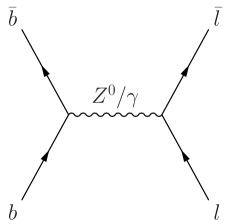
$\oplus$

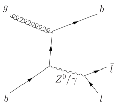
$\ominus$

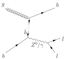
Figure 4: Representative Feynman diagrams for the Drell-Yan with associated b-quark production process for (from left to right): Order $\rm\alpha_{s}^{(0)}$, order $\rm\alpha_{s}^{(1)}$ and order $\rm\alpha_{s}^{(1)}$ subtraction term.

Table 1: The process cross-sections for the leading order process $b\bar{b}\to Z\to\mu^{+}\mu^{-}$, next-to-leading order process $gb\to Zb\to\mu^{+}\mu^{-}b$ and the subtraction process $(g\to b\bar{b})b\to Zb\to\mu^{+}\mu^{-}b$ in the LHC environment (proton-proton collisions at $\rm\sqrt{s}$ = 14 TeV) are listed. The b-quark mass is set to $m_{b}=4.8$ GeV and the factorization and renormalization scales are set to the $Z^{0}$ invariant mass squared. In addition, the order $\rm\alpha_{s}^{(2)}$ $gg\to Zb\bar{b}\to\mu^{+}\mu^{-}b\bar{b}$ process cross-section is shown for comparison. The cross-sections are given for the LO CTEQ5L [26] and the derived JCC PDFs. In the Monte-Carlo procedure the next-to-leading process weights are combined with the subtraction weights on the event-by-event basis as described in the text.

Process	$\sigma_{\mathrm{CTEQ5L,\mu_{0}=m_{Z}}}$ $\rm[pb]$	$\sigma_{\mathrm{JCC,\mu_{0}=m_{Z}}}$ $\rm[pb]$
$b\bar{b}\to Z\to\mu^{+}\mu^{-}$	57.9	39.9
$gb\to Zb\to\mu^{+}\mu^{-}b$	72.1	60.0
$(g\to b\bar{b})b\to Zb\to\mu^{+}\mu^{-}b$	73.3	60.9
$\Sigma$	56.7	39.0
$gg\to Zb\bar{b}\to\mu^{+}\mu^{-}b\bar{b}$	22.8	22.8

The cross-sections obtained for the leading order process $b\bar{b}\to Z\to\mu^{+}\mu^{-}$, next-to-leading order process $gb\to Zb\to\mu^{+}\mu^{-}b$ and the subtraction process $(g\to b\bar{b})b\to Zb\to\mu^{+}\mu^{-}b$ in the LHC environment (proton-proton collisions at $\rm\sqrt{s}$ = 14 TeV) are given in the Table 1, both for leading order PDF (CTEQ5L [26] was used) and the PDF-s evolved according to the Collins prescription (c.f. Equation 2.2, labeled JCC), along with the cross-section for the order $\rm\alpha_{s}^{(2)}$ $gg\to Zb\bar{b}\to\mu^{+}\mu^{-}b\bar{b}$ process. Separate cross-section contributions for the next-to-leading order process and the subtraction term are given for convenience; in the Monte-Carlo procedure developed in this paper the events are generated according to the differential cross-section corresponding to the ’hard’ order $\alpha_{s}^{(1)}$ process, i.e. the next-to-leading calculation with the subtraction terms subtracted on an event-by-event basis.

The differential distributions of the virtuality $\rm\mu$ and the transverse momentum ($p_{T}$) distribution of the b-quark with the highest $p_{T}$ of the two (produced either in the hard process or in the subsequent Sudakov showering) are shown in Figure 5, whereby also the $p_{T}$ distribution of the b-quark with the highest $p_{T}$ from the order $\rm\alpha_{s}^{(2)}$ $gg\to Zb\bar{b}\to\mu^{+}\mu^{-}b\bar{b}$ process is shown.

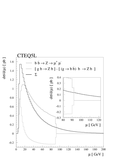
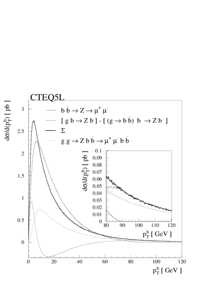
Figure 5: The differential distributions of the virtuality $\rm\mu$ and the transverse momentum ($p_{T}$) distribution of the b-quark with the higher virtuality (produced either in the hard process or in the subsequent Sudakov showering) are shown for the calculations using the LO CTEQ5L parton density functions. The next-to-leading order process entries contain the subtraction terms as calculated on event-by event basis.

In the results in Fig. 5 one can observe a smooth distribution of the virtuality $\rm\mu$ over the full kinematic range as the result of the implemented matching procedure. It is manifest that the cutoff on the b-quark virtuality $\mu$ and the resulting subtraction contribution do not map to the $p_{T}$ distribution in a simple way. An interesting result is that the order $\rm\alpha_{s}^{(2)}$ $gg\to Zb\bar{b}\to\mu^{+}\mu^{-}b\bar{b}$ process $p_{T}$ distribution of the b-quark seems to be quite close to the result of the merging procedure in the high kinematic range as one could indeed expect if the perturbative calculations are to be consistent in the perturbative regime. In the low $p_{T}$ region the $gg\to Zb\bar{b}\to\mu^{+}\mu^{-}b\bar{b}$ process undershoots the expected distribution of the merged $\rm\alpha_{s}^{(0)}\oplus\rm\alpha_{s}^{(1)}$ processes which is to be expected since in this case the non-perturbative contributions prevail. One has to keep in mind when comparing the two results results that in the derived $\rm\alpha_{s}^{(1)}$ calculation the other incoming b-quark is still effectively on-shell, i.e. its virtuality and branchings are obtained solely from the Sudakov showering, where as in the $\rm\alpha_{s}^{(2)}$ process both incoming b-quarks are treated as propagators in the full perturbative calculation. A further improvement would certainly be to repeat and extend the procedures derived in this paper to include the full order $\rm\alpha_{s}^{(2)}$ calculation.

From the results one can also see that the use of JCC evolved PDF-s significantly reduces the cross-section of the leading-order process with respect to the values obtained using the CTEQ5L [26] PDFs and to a lesser extent the cross-sections of the next-to-leading and the subtraction contribution, since the latter two include only one b-quark and one gluon in the initial state and are thus less affected by the change in the b-quark PDF evolution.

3.2 The ’t-channel’ Single Top Production Process

The ’t-channel’ single top production mechanism is of importance at the LHC since it provides a clean signal for top quark and W boson polarization studies. The final state consist of a $t,W$, and $\overline{b}$ as illustrated in Fig. 6

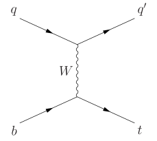
$\oplus$

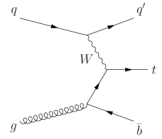
$\ominus$

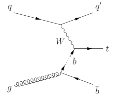
Figure 6: Representative Feynman diagrams for the ’t-channel’ single top production process for (from left to right): Order $\rm\alpha_{s}^{(0)}$, order $\rm\alpha_{s}^{(1)}$ and order $\rm\alpha_{s}^{(1)}$ subtraction term.

The cross-sections obtained for the leading order process $bq\to tq^{\prime}$, next-to-leading order process $gq\to tq^{\prime}\bar{b}$ and the subtraction process $(g\to b\bar{b})q\to tq^{\prime}\bar{b}$ (and charge conjugates) in the LHC environment (proton-proton collisions at $\rm\sqrt{s}$ = 14 TeV) are given in the Table 2, both for leading order PDF (CTEQ5L [26] was used) and the PDF-s evolved according to the Collins prescription (c.f. Equation 2.2, labeled JCC) for the scale choices $\rm\mu_{0}=m_{t}$ and $\rm\mu_{0}=60~{}GeV$. The differential distributions of the virtuality $\rm\mu$ and the transverse momentum ($p_{T}$) distribution of the b-quark (produced either in the hard process or in the subsequent Sudakov showering) are shown in Figures 7 and 8. Separate cross-section contributions are given for convenience; in the Monte-Carlo procedure developed in this paper the $gq\to tq^{\prime}\bar{b}$ events are generated according to the differential cross-section corresponding to the ’hard’ order $\alpha_{s}^{(1)}$ process, i.e. the next-to-leading calculation with the subtraction terms subtracted on an event-by-event basis.

Table 2: The process cross-sections for the leading order process $bq\to tq^{\prime}$, next-to-leading order process $gq\to tq^{\prime}\bar{b}$ and the subtraction process $(g\to b\bar{b})q\to tq^{\prime}\bar{b}$ (including the charge conjugates) in the LHC environment (proton-proton collisions at $\rm\sqrt{s}$ = 14 TeV) are listed. These inclusive cross-sections include all top (and $W^{\pm}$) decay channels, the b-quark mass is set to $m_{b}=4.8$ GeV and top-quark mass to $m_{t}=175$ GeV with the factorization and renormalization scales set to the top mass values $\rm\mu_{0}=m_{t}$ and $\rm\mu_{0}=60~{}GeV$. The cross-sections are given for the LO CTEQ5L and JCC PDFs. In the Monte-Carlo procedure the next-to-leading process weights are combined with the subtraction weights on the event-by-event basis as described in the text.

Process	$\sigma_{\mathrm{CTEQ5L,\atop\mu_{0}=m_{t}}}$ $\rm[pb]$	$\sigma_{\mathrm{JCC,\atop\mu_{0}=m_{t}}}$ $\rm[pb]$	$\sigma_{\mathrm{CTEQ5L,\atop\mu_{0}=60~{}GeV}}$ $\rm[pb]$	$\sigma_{\mathrm{JCC,\atop\mu_{0}=60~{}GeV}}$ $\rm[pb]$
$bq\to tq^{\prime}$	222.2	187.8	178.1	138.7
$gq\to tq^{\prime}\bar{b}$	156.2	154.2	188.2	184.4
$(g\to b\bar{b})q\to tq^{\prime}\bar{b}$	140.1	138.2	102.8	100.5
$\Sigma$	238.3	203.8	263.5	222.6

From the results in Fig. 7 and Fig. 8 one can observe that the applied procedure produces a very good match of the processes in the combined distribution of the b-quark virtuality $\mu$ resulting in a smooth (almost seamless) transition in the vicinity of the cutoff. As one can also observe the cutoff on the b-quark virtuality $\mu$ and the resulting subtraction contribution do not map to the $p_{T}$ distribution in a trivial manner; hence one can surmise that the simple methods involving adding of the processes based on $p_{T}$ distribution cuts probably give erroneous predictions.

This procedure can in unmodified form be applied to the full $2\to 4$ and $2\to 4$ matrix elements $bq\to tq^{\prime}\to Wbq^{\prime}\to f\bar{f}^{\prime}bq$ and $gq\to tq^{\prime}\bar{b}\to Wbq^{\prime}\bar{b}\to f\bar{f}^{\prime}bq\bar{b}$ including top quark decays and has as such also been implemented in the AcerMC Monte-Carlo generator.

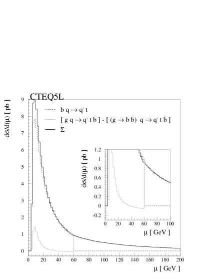
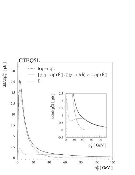
Figure 7: The differential distributions of the virtuality $\rm\mu$ and the transverse momentum ($p_{T}$) distribution of the b-quark (produced either in the hard process or in the subsequent Sudakov showering) are shown for the calculations using the LO CTEQ5L PDFs and the showering (factorization) scale set to $\rm\mu_{0}=60~{}GeV$. The next-to-leading order process entries contain the subtraction terms as calculated on event-by event basis.

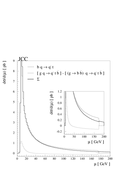
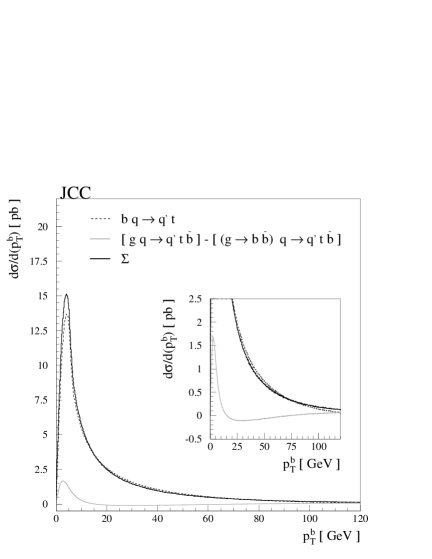
Figure 8: The differential distributions of the virtuality $\rm\mu$ and the transverse momentum ($p_{T}$) distribution of the b-quark (produced either in the hard process or in the subsequent Sudakov showering) are shown for the calculations using the JCC PDFs and the showering (factorization) scale set to $\rm\mu_{0}=m_{t}$. The next-to-leading order process entries contain the subtraction terms as calculated on event-by event basis.

One of the interesting results is that the use of JCC evolved PDF-s significantly reduces the cross-section of the $bq\to tq^{\prime}$ process with respect to the values obtained using the CTEQ5L PDFs and to a lesser extent the cross-sections of the $gq\to tq^{\prime}\bar{b}$ and the subtraction contribution, since the latter two contain only the light quarks and gluons which are less (or in case of gluons not at all) affected by the change in PDF evolution compared to the b-quark PDF.

A somewhat cruder method of merging different order processes has for the ’t-channel’ single top production already been implemented a while ago in the program ONETOP[27]; the results from the two methods are compatible within the differences of the methods used in both implementations. It is instructive to understand where the differences between the two procedures originate. Specifically, in ONETOP the subtraction term is higher than the cross-section of the $(2\to 3)$ $gq\to tq^{\prime}\bar{b}$ process; from the Fig. 3.6 in [27] the subtraction cross-section of the process $(g\to b\bar{b})q\to tq^{\prime}\bar{b}$ is of the order of about 190 pb compared to the 140 pb one gets using the procedures described in this paper. The difference originates in part in the massless approximation of the participating particles implemented in ONETOP and can be traced back to the fact that the subtraction term in ONETOP (as given in Appendix D in [27]) is calculated from the integrated parton density function correction (the first-order term in Eq. 12 of this paper) coupled to the zero-th order $bq\to tq^{\prime}$ cross-section, since the virtuality is already integrated over into the $\log\frac{\mu^{2}}{m_{b}^{2}}$. In contrast, in the present work the procedure is more complex and requires identifying the virtuality of the $2\to 3$ process in the massive calculation. In addition, in ONETOP the spectator energy fraction is kept unchanged whereas in the new procedure only the rapidity constraint is used instead. The ONETOP calculation using the integrated PDF correction has been repeated as a check and gives a subtraction term with the value of about 185 pb which is consistent with the ONETOP results.

3.3 The ’tW channel’ Single Top Production Process

The ’tW-channel’ single top production mechanism is also of importance at the LHC since it provides a clean signal for top quark and W boson polarization studies. The process is illustrated in Fig. 9.

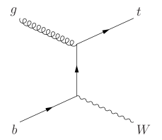
$\oplus$

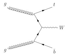
$\ominus$

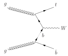
Figure 9: Representative Feynman diagrams for the ’tW-channel’ single top production process for (from left to right): Order $\rm\alpha_{s}^{(0)}$, order $\rm\alpha_{s}^{(1)}$ and order $\rm\alpha_{s}^{(1)}$ subtraction term.

The cross-sections obtained for the leading order process $gb\to t(W\to)f\bar{f}^{\prime}$, next-to-leading order process $gg\to t(W\to)f\bar{f}^{\prime}\bar{b}$ and the subtraction process $(g\to b\bar{b})g\to t(W\to)f\bar{f}^{\prime}\bar{b}$ (and charge conjugates) at the LHC. are given in the Table 3, both for leading order PDF (CTEQ5L [26] was used) and the PDF-s evolved according to the Collins prescription (c.f. Equation 2.2, labeled JCC) for the scale choice $\rm\mu_{0}=60~{}GeV$. The differential distributions of the virtuality $\rm\mu$ and the transverse momentum ($p_{T}$) distribution of the b-quark (produced either in the hard process or in the subsequent Sudakov showering) are shown in the Figure 10 . Separate cross-section contributions are given for convenience; in the Monte-Carlo procedure developed in this paper the $gg\to t(W\to)f\bar{f}^{\prime}\bar{b}$ events are generated according to the differential cross-section corresponding to the ’hard’ order $\alpha_{s}^{(1)}$ process, i.e.   the next-to-leading calculation with the subtraction terms subtracted on an event-by-event basis. Note also that in this case there are indeed two subtraction terms, one for each incoming gluon.

From the results in Fig. 10 one can again observe that the applied procedure produces a very good match of the processes in the combined distribution of the b-quark virtuality $\mu$ resulting in a smooth (almost seamless) transition in the vicinity of the cutoff. As one can also observe the cutoff on the b-quark virtuality $\mu$ and the resulting subtraction contribution do again not map to the $p_{T}$ distribution in a trivial manner; again therefore one expects that the simple gluing methods of the processes based on $p_{T}$ distribution cuts most probably give erroneous predictions.

Table 3: The process cross-sections for the leading order process $gb\to t(W\to)f\bar{f}^{\prime}$ , next-to-leading order process $gg\to t(W\to)f\bar{f}^{\prime}\bar{b}$ and the subtraction process $(g\to b\bar{b})g\to t(W\to)f\bar{f}^{\prime}\bar{b}$ (including the charge conjugates) in the LHC environment (proton-proton collisions at $\rm\sqrt{s}$ = 14 TeV) are listed. These inclusive cross-sections include all top decay channels, the associated $W^{\pm}$ decays into muon and neutrino and the b-quark mass is set to $m_{b}=4.8$ GeV and top-quark mass to $m_{t}=175$ GeV with the factorization and renormalization scales set to the $\rm\mu_{0}=60~{}GeV$. The cross-sections are given for the LO CTEQ5L and JCC PDFs. In the Monte-Carlo procedure the next-to-leading process weights are combined with the subtraction weights on the event-by-event basis as described in the text.

Process	$\sigma_{\mathrm{CTEQ5L,\mu_{0}=60~{}GeV}}$ $\rm[pb]$	$\sigma_{\mathrm{JCC,\mu_{0}=60~{}GeV}}$ $\rm[pb]$
$gb\to t(W\to)\mu\bar{\nu}_{\mu}$	5.9	4.7
$gg\to t(W\to)\mu\bar{\nu}_{\mu}\bar{b}$	6.0	6.0
$(g\to b\bar{b})g\to t(W\to)\mu\bar{\nu}_{\mu}\bar{b}$	3.1	3.1
$\Sigma$	8.8	7.6

The diagrams of the process $gg\to tWb\to WWb\bar{b}\to ffffb\bar{b}$ are in fact just a subset of 31 Feynman diagrams which have a $WWb\bar{b}$ intermediate state (and which also include the $t\bar{t}$ production). Accordingly, the derived subtraction procedure has in, AcerMC, been applied to the processes having the full set of Feynman diagrams and the above plots and values should be considered only as the validation of the procedure in case of the ’tW channel’ single top production.

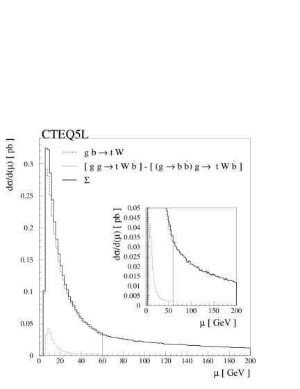
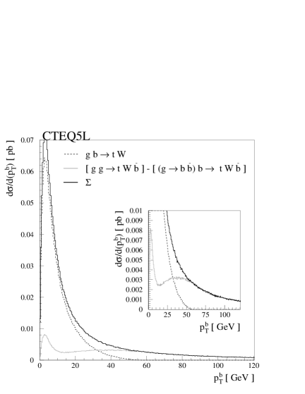
Figure 10: The differential distributions of the virtuality $\rm\mu$ and the transverse momentum ($p_{T}$) distribution of the b-quark (produced either in the hard process or in the subsequent Sudakov showering) are shown for the calculations using the LO CTEQ5L PDFs and the showering (factorization) scale set to $\rm\mu_{0}=60~{}GeV$. The next-to-leading order process entries contain the subtraction terms as calculated on event-by event basis.

4 Conclusion

It has been demonstrated explicitly how to deal with the case where a particle of interest can be produced from a partonic hard scattering process or as a remnant of an incoming hadron beam. Examples of the proceedure have been provided and contrasted with the more ad-hoc proceedures used previously to prevent double counting.

Appendix A Kinematic Relations

The requirement (2) in the list of Subsection 2.1 gives the equivalence $\rm\xi_{a}\equiv x_{a}$. The remaining relations between $\rm\xi_{c},\xi_{b}$ and $x_{b},s_{n-1}$ are then given by energy and rapidity conservation requirements and are thus given by the conditions:

$$s_{n-1}=(p_{c}+p_{b})^{2}=m_{c}^{2}+m_{b}^{2}+2(p_{c}^{+}p_{b}^{-}+p_{c}^{-}p_{b}^{+})=m_{c}^{2}+m_{b}^{2}+\xi_{c}\xi_{b}s+\frac{m_{c}^{2}m_{b}^{2}}{\xi_{c}\xi_{b}s}$$ (30)

where $p_{c}=(p_{c}^{+},\vec{0}^{T},p_{c}^{-})=(\xi_{c}P_{A}^{+},\vec{0}^{T},\frac{m_{c}^{2}}{2\xi_{c}P_{A}^{+}})$ and $p_{b}=(p_{b}^{+},\vec{0}^{T},p_{b}^{-})=(\frac{m_{b}^{2}}{2\xi_{b}P_{B}^{-}},\vec{0}^{T},\xi_{b}P_{B}^{-})$ and:

$$y=\frac{1}{2}\ln\left(\frac{k_{n-1}^{+}}{k_{n-1}^{-}}\right)=\frac{1}{2}\ln\left(\frac{\xi_{c}}{\xi_{b}}\right)+\frac{1}{2}\ln\left(\frac{\xi_{c}\xi_{b}s+m_{b}^{2}}{\xi_{c}\xi_{b}s+m_{c}^{2}}\right)$$ (31)

with:

$$\frac{k_{n-1}^{+}}{k_{n-1}^{-}}=\left(\frac{1+\beta}{1-\beta}\right)\left(\frac{k_{n-1}^{+*}}{k_{n-1}^{-*}}\right)~{}~{}~{}~{}~{}~{}~{}\left(\frac{1+\beta}{1-\beta}\right)=\frac{x_{a}(x_{a}x_{b}s+m_{b}^{2})}{x_{b}(x_{a}x_{b}s+m_{a}^{2})}$$ (32)

and:

$$k_{n-1}^{\pm\star}=\frac{1}{\sqrt{2}}\left[\frac{s_{n}+s_{n-1}-m_{\bar{c}}^{2}}{2\sqrt{s_{n}}}\mp\frac{t_{n-1}-m_{b}^{2}-s_{n-1}+2\left(\frac{s_{n}+m_{b}^{2}-m_{a}^{2}}{2\sqrt{s_{n}}}\right)\left(\frac{s_{n}+s_{n-1}-m_{\bar{c}}^{2}}{2\sqrt{s_{n}}}\right)}{2\left(\frac{\sqrt{\lambda(s_{n},m_{a}^{2},m_{b}^{2})}}{2\sqrt{s_{n}}}\right)}\right]$$ (33)

which can be inverted to give the expressions for $\xi_{c}$ and $\xi_{b}$ as functions of $s_{n},x_{b},\ldots$ A further simplification in derivation can be achieved by introducing another set of variables $\bar{\tau}=\xi_{c}\cdot\xi_{b}$ and $\bar{y}=1/2\ln(\xi_{c}/\xi_{b})$ with the Jacobian of the transformation $\mathcal{J}\frac{(\xi_{c},\xi_{b})}{(\bar{\tau},\bar{y})}=1$ and subsequently:

$$\bar{\tau} = \frac{1}{2s}\left\{\left(s_{n-1}-(m_{c}^{2}+m_{b}^{2})\right)+\sqrt{\lambda(s_{n-1},m_{c}^{2},m_{b}^{2})}\right\},$$ (34)

$$\bar{y} = \frac{1}{2}\ln\left(\frac{k_{n-1}^{+}}{k_{n-1}^{-}}\right)-\frac{1}{2}\ln\left(\frac{\bar{\tau}s+m_{b}^{2}}{\bar{\tau}s+m_{c}^{2}}\right).$$ (35)

As one can observe the $\bar{\tau}$ is only a function of $s_{n-1}$ so the only remaining term to compute in the Jacobian of the transformation $\mathcal{J}\frac{(\bar{\tau},\bar{y})}{(s_{n-1},x_{b})}$ is $d\bar{y}/dx_{b}$:

$$\mathcal{J}\frac{(\bar{\tau},\bar{y})}{(s_{n-1},x_{b})}=\left|\frac{d\bar{\tau}}{ds_{n-1}}\right|\cdot\left|\frac{d\bar{y}}{dx_{b}}\right|=\mathcal{F}(s_{n},s_{n-1},t_{n-1},x_{a},x_{b},m_{a},m_{b},m_{\bar{c}})$$ (36)

with $\mathcal{F}$ being a lengthy function of the listed parameters and therefore omitted. In the massless approximation the above expression reduces to:

$$\mathcal{J}\frac{(\xi_{c},\xi_{b})}{(s_{n-1},x_{b})}_{m\to 0}=\left|\frac{x_{a}}{2(x_{a}x_{b}s+t_{n-1})}+\frac{1}{2x_{b}s}\right|$$ (37)

which is in agreement with the expressions derived by Chen, Collins et al. [9, 10, 11, 12]. Analogous expressions can trivially be obtained also for the split of the other parton.

References

- [1] G. Altarelli and G. Parisi, Nucl. Phys. B 126 (1977) 298
- [2] J. C. Collins and D. E. Soper, Phys. Rev. D 16 (1977) 2219
- [3] J. C. Collins and D. E. Soper, Nucl. Phys. B 194 (1982) 445
- [4] J. C. Collins, Phys. Rev. D 58 (1998) 094002 [hep-ph/9806259].
- [5] F. I. Olness and W. K. Tung, OITS-426 Published in Proc. of 12th Warsaw Symp. on Elementary Particle Physics, Kazimierz, Poland, May 29 - Jun 2, 1989
- [6] M. A. G. Aivazis, F. I. Olness and W. K. Tung, Phys. Rev. D 50 (1994) 3085 [hep-ph/9312318].
- [7] M. A. G. Aivazis, J. C. Collins, F. I. Olness and W. K. Tung, Phys. Rev. D 50 (1994) 3102 [hep-ph/9312319].
- [8] F. I. Olness, R. J. Scalise and W. K. Tung, Phys. Rev. D 59 (1999) 014506 [hep-ph/9712494].
- [9] J. C. Collins, J. High Energy Phys. 0005 (2000) 004 [hep-ph/0001040].
- [10] Y. j. Chen, J. Collins and X. m. Zu, J. High Energy Phys. 0204 (2002) 041 [hep-ph/0110257].
- [11] Y. Chen, J. C. Collins and N. Tkachuk, J. High Energy Phys. 0106 (2001) 015 [hep-ph/0105291].
- [12] J. C. Collins and X. m. Zu, J. High Energy Phys. 0206 (2002) 018 [hep-ph/0204127].
- [13] S. Catani, F. Krauss, R. Kuhn and B. R. Webber, J. High Energy Phys. 0111 (2001) 063 [hep-ph/0109231].
- [14] S. Mrenna and P. Richardson, J. High Energy Phys. 0405 (2004) 040 [hep-ph/0312274].
- [15] T. Sjostrand, L. Lonnblad and S. Mrenna, [hepph0108264].
- [16] B. P. Kersevan and E. Richter-Was, Eur. Phys. J. C 39 (2005) 439 [hep-ph/0405248].
- [17] B. P. Kersevan and E. Richter-Was, Comput. Phys. Commun. 149 (2003) 142 [hep-ph/0201302].
- [18] E. Byckling and K. Kajantie, Nucl. Phys. B 9 (1969) 568 E. Byckling and K. Kajantie, “Particle Kinematics”, Wiley & Sons. , London (1973) 328p.
- [19] P. J. Sutton, A. D. Martin, R. G. Roberts and W. J. Stirling, Phys. Rev. D 45 (1992) 2349
- [20] P. J. Rijken and W. L. van Neerven, Phys. Rev. D 52 (1995) 149 [hep-ph/9501373].
- [21] D. A. Kosower and P. Uwer, Nucl. Phys. B 674 (2003) 365 [hep-ph/0307031].
- [22] S. Moch, J. A. M. Vermaseren and A. Vogt, Nucl. Phys. B 646 (2002) 181 [hep-ph/0209100].
- [23] P. J. Rijken and W. L. van Neerven, Phys. Rev. D 51 (1995) 44 [hep-ph/9408366].
- [24] W. K. Tung, S. Kretzer and C. Schmidt, J. Phys. G 28 (2002) 983 [hep-ph/0110247].
- [25] M. Bengtsson and T. Sjostrand, Z. Physik C 37 (1988) 465
- [26] H. L. Lai et al. [CTEQ Collaboration], Eur. Phys. J. C 12 (2000) 375 [hep-ph/9903282].
- [27] D. O. Carlson, [hep-ph/9508278].