Key words: $\pi K$ scatterings, Unitarity, Dispersion relations
PACS number: 14.40.Ev, 13.85.Dz, 11.55.Bq, 11.30.Rd

The debate on whether there exists a $\kappa$ meson in the I,J=1/2,0 channel $\pi K$ scattering process has a rather long history. [2, 3] In a previous paper [4] we studied the problem on the existence of the $\kappa$ resonance and have concluded, based on the LASS phase shift data on $\pi K$ scatterings, [1] that the $\kappa$ resonance should exist if the scattering lengths are close to those predicted by $\chi$PT. [5] The conclusion is obtained using a new parametrization form for the elastic scattering amplitude respecting unitarity and analyticity. [4] It should be emphasized that one only needs to assume the validity of Mandelstam representation in order to establish the parametrization form (herewith called the PKU parametrization form). One of the most remarkable advantages of the PKU form is that the effects of the elastic unitarity cut are dissolved into (2nd sheet) pole contributions and more distant cut contributions. It can still keep track of contributions from distant cuts which is of great help in stablizing the fit $\kappa$ pole location, [6] comparing with the conventional $K$–matrix approach. Meanwhile the pole location is not sensitive to the details of the input left hand cut (in Ref. [4] 1–loop $\chi$PT estimates on the left hand cut was used) and hence the theoretical uncertainties are severely suppressed. The PKU parametrization form is found to be sensitive to low lying isolated singularities not too far away from the elastic threshold and hence provides a powerful tool especially in exploring those light and broad resonances.

The PKU parametrization form for the partial wave elastic scattering $S$ matrix is, [4]

$$S^{phy.}=\prod_{i}S^{R_{i}}\times S^{cut}\ ,$$ (1)

where $S^{R_{i}}$ denotes the (second sheet) pole contribution, since there are no bound state poles in $\pi K$ scatterings. $S^{cut}=e^{2i\rho f(s)}$ represents the cut contribution and $f(s)$ can be expressed as

$$f(s) = f(s_{0})+{(s-s_{0})\over 2\pi i}{\int_{C}}{{\mathrm{disc}f(z)\over{(z-s)(z-s_{0})}}dz}+{(s-s_{0})\over\pi}{\int_{L_{1}+L_{2}}}{{\mathrm{Im_{L}}f(z)\over{(z-s)(z-s_{0})}}dz}$$ (2)

$$+ {(s-s_{0})\over\pi}{\int_{R}}{{\mathrm{Im_{R}}f(z)\over{(z-s)(z-s_{0})}}dz}\ ,$$

where $L_{1}$ denotes the left hand cut on the real axis from -$\infty$ to $-(m_{K}^{2}-m_{\pi}^{2})$, $L_{2}$ denotes the left hand cut from $-(m_{K}^{2}-m_{\pi}^{2})$ to $(m_{K}-m_{\pi})^{2}$, $C$ is the circular cut, and $R$ denotes cuts from the first inelastic threshold to $+\infty$. See Fig. 1 for explanation.

Figure 1: The left hand cut, circular cut and the right hand cut of partial wave $\pi K$ scattering amplitudes.

The discontinuity of $f$ on each cut obeys the following formula,

$$\mbox{disc}f(s)=\mbox{disc}\{\frac{1}{2i\rho(s)}\log[S^{phy}(s)]\}\ .$$ (3)

The cut structure of function $f(s)$ as depicted in Fig. 1 is generated by the partial wave projection of the un-equal mass elastic scatterings: [7]

$$T^{I}_{J}(s)={1\over 32\pi}\int_{-1}^{1}d({\mathrm{cos}\theta})P_{J}(\mathrm{cos}\theta)T^{I}(s,t,u)\ ,$$ (4)

where

$$\mathrm{cos}\theta = 1+{{t}\over{2{q_{s}}^{2}}}\ ,$$

$$q_{s} = ({(s-(m_{K}+m_{\pi})^{2})(s-(m_{K}-m_{\pi})^{2})\over{4s}})^{1/2}\ ,$$

$$u = 2m_{K}^{2}+2m_{\pi}^{2}-s-t\ .$$ (5)

For the convenience of further discussions Eq. (4) is rewritten as

$$T^{I}_{J}(s) = {1\over 32\pi}{1\over 2{q_{s}}^{2}}\int_{-4{q_{s}}^{2}}^{0}dtP_{J}(1+{{t}\over{2{q_{s}}^{2}}})T^{I}(s,t,u)\ .$$ (6)

In Eq. (2) there is an arbitrary subtraction constant $f(s_{0})$. In Ref. [8] when discussing $\pi\pi$ scatterings it was observed that if taking the subtraction at $s=0$ then one can use the property $T^{I}_{J}(0)=const$ to fix the arbitrary subtraction constant: $f(0)=0$. For unequal mass scatterings, however, the situation becomes more complicated. The simple argument given in Ref. [8] which led to $f(0)=0$ has to be modified here. It is easy to understand this when looking at Eq. (6): when taking for example the $s\to 0$ limit one has

$$q_{s}^{2}\to\frac{(M_{K}^{2}-m_{\pi}^{2})^{2}}{4}s^{-1}\to\infty\ .$$ (7)

Therefore in order to reveal the singularity structure of $T^{I}_{J}(s)$ when $s\to 0$ one has to evaluate the integral in Eq. (4) which has to be performed from $t=0$ to $-\infty$. Hence the asymptotic behavior of $T^{I}_{J}(s)$ when $s\to 0$ depends on the asymptotic behavior of the isospin amplitude $T^{I}(s,t)$ when $s\to 0$, $t\to\infty$, and the latter is the energy region governed by Regge model. In Ref. [9] a similar problem for $\pi N$ scattering has been studied by assuming a high energy Regge behavior of $T^{I}(s,t)$ and it is obtained that $T^{I}_{J}\to s^{-|const|}$ when $s\to 0$, depending on the leading Regge exchanges in crossed channels. Nevertheless it is not clear whether the low partial wave projections of Regge amplitudes should be totally trustworthy [10] and therefore we will not adopt such an analysis here. We simply point out here that if assuming the polynomial boundedness of the isospin amplitude: $|T^{I}(s,t)|<|t|^{n}$ when $|t|\to\infty$ and $s$ fixed (which is a consequence of Mandelstam analyticity), then $T^{I}_{J}(0)$ will be singular at most of order $s^{-n}$. The latter is enough for the purpose to fix the subtraction constant in the present problem. To see this, we evaluate the asymptotic behavior of

$$\frac{1}{2i\rho(s)}\log(1+2i\rho(s)T^{phy}(s))=\frac{1}{2i\rho(s)}\sum_{i}\log(S^{R_{i}}(s))+f(s)\ .$$ (8)

When $s\rightarrow 0$, $\rho(s)=2q_{s}/\sqrt{s}\sim s^{-1}$. Now if $T^{phy}(s)\sim O(s^{-n})$, the left hand side vanishes when $s\rightarrow 0$, and it leads to

$$f(0)=0\ ,\\$$ (9)

on the $r.h.s.$. The condition Eq. (9) should be true at least for finite number of poles, as a self-consistency requirement of our approximation scheme. Thus the dispersion relation Eq. (2) is simplified as,

$$f(s) = {s\over 2\pi i}{\int_{C}}{{\mathrm{disc}f(z)\over{(z-s)z}}dz}+{s\over\pi}{\int_{L_{1}+L_{2}}}{{\mathrm{Im_{L}}f(z)\over{(z-s)z}}dz}+{s\over\pi}{\int_{R}}{{\mathrm{Im_{R}}f(z)\over{(z-s)z}}dz}\ .$$ (10)

Since there is no bound state pole in $\pi K$ scatterings Eq. (10) can be recasted as a more compact form,

$$f(s) = {s\over 2\pi i}{\int_{C_{o}}}{{f(z)\over{(z-s)z}}dz}+{s\over\pi}{\int_{L_{1}}}{{\mathrm{Im_{L}}f(z)\over{(z-s)z}}dz}+{s\over\pi}{\int_{R}}{{\mathrm{Im_{R}}f(z)\over{(z-s)z}}dz}$$ (11)

when $s$ lies outside the circular cut. Different from conventional dispersion relations, the integrand appeared in Eq. (11) is logarithmic. This is a remarkable property when we use chiral perturbation theory results to approximate $S^{phy}$ in Eq. (3), since the bad high energy behavior of chiral expansions is severely suppressed. As a consequence, in the I=1/2 channel it is found that [4] the physical outputs are not sensitive to the details of the left hand cut contribution at all. Similar situation happens in the studies of the I=0, J=0 channel $\pi\pi$ scattering. [8] What is truly important to introduce the estimation on the left hand cut when studying the low lying broad resonance is, as revealed in Ref. [11], that the left hand cut contribution to the phase shift is negative and concave, hence the $\kappa$ ($\sigma$) pole has to be introduced in order to saturate the experimental data. The observation that the background contributions are negative and concave as obtained by using chiral perturbation theory may be doubtful as the latter does not work at high energies. Nevertheless we believe that the observed qualitative behavior of the background contribution has little to do with the bad high energy behavior of chiral amplitudes. There are two reasons: first of all, as can be verified from Eqs. (11) and (3), as long as $|S^{phy}|>1$, the left hand cut contribution to the phase shift is always negative and concave. But elastic scattering amplitudes are dominated by pomeron exchanges at high energies which naturally satisfy $|S^{phy}|>1$. The second reason is that, at moderately high energies on the left side, one may expect that results from chiral perturbation theory are not as bad as it behaves on the right hand side. Because there is no unitarity constraints on the left. Also the left hand side is further away from resonance (which is one of the main reason for chiral perturbation theory to break down) region and on the left side pole singularities are converted to much mild cut singularities.

In Ref. [4] a fit to the LASS data up to 1.43 GeV was performed with seven parameters. Six of them are used by MINUIT: two for the $\kappa$ pole, two for $K_{0}^{*}(1430)$ pole and two scattering lengths (or equivalently the two subtraction constants), $a^{1/2}_{0}$ and $a^{3/2}_{0}$. In addition there is another manually tuned cutoff parameter $\Lambda_{L}^{2}$ being responsible for the truncation of the left hand cut integral, chosen at $\Lambda^{2}_{L}\simeq 1.5$GeV². The cutoff parameters in the I=1/2 channel and in the I=3/2 channel were chosen to be equal, and the value was fixed for getting a minimal $\chi^{2}$ in Eq. (48) of Ref. [4]. The two scattering lengths are free parameters in Ref. [4]. In here according to previous discussions, the scattering lengths are no longer free. In the following we present the numerical fit results with six parameters: two for the $\kappa$ pole, two for the $K_{0}^{*}(1430)$ pole, one cutoff parameter in the I=1/2 channel and one in the I=3/2 channel. Other conditions are the same as those led to Eq. (48) of Ref. [4] for convenience of comparison, but remembering that now we use instead Eq. (11). The results are listed below:

$$\chi^{2}_{d.o.f.}=80.3/(60-6)\ ;$$

$$M_{\kappa}=694\pm 53MeV\ ,\,\,\,\Gamma_{\kappa}=606\pm 59MeV\ ;$$

$$M_{K^{II}_{0}(1430)}=1443\pm 15MeV\ ,\,\,\,\Gamma_{K^{II}_{0}(1430)}=199\pm 35MeV\ ;$$ (12)

with $\Lambda_{1/2}^{2}=-13.6\pm 40.0$GeV², $\Lambda_{3/2}^{2}=-11.4\pm 1.7$Gev². Also a calculation gives

$$a^{1/2}_{0}=0.219\pm 0.034\ ,\,\,\,a^{3/2}_{0}=-0.042\pm 0.002\ .$$ (13)

From the above results we observe that, first of all, unlike Ref. [4] where one finds, if taking the scattering lengths to be totally free, a much better $\chi^{2}$ fit to the data can be gained with considerably larger (in magnitude) scattering length parameters, at the cost of introducing an essential singularity at $s=0$. The better use of the analyticity property seems to further suggest that the low energy LASS data, to some extent, conflict other results based on chiral symmetry and $S$ matrix theory. Nevertheless the existence of $\kappa$ resonance is undoubted within the present scheme. For example, if freezing one pole the fit gives $\chi^{2}_{d.o.f.}=1055.0/(60-4)$. It is worth emphasizing again that the present scheme indicates, even using the LASS data, that the threshold parameters are in good agreement with results obtained using chiral symmetry and $S$ matrix theory properties, for example, the Roy–Steiner equations [13] and also the dispersive approach of Ref. [14]. The effective range parameters are found to be $b^{1/2}_{0}=0.075\pm 0.023$ and $b^{3/2}_{0}=-0.027$, which also agree fairly well with the results given in Ref. [13], despite that the present $b^{3/2}_{0}$ contains a too small error bar. It is also worth pointing out that the large error bar of $\Lambda_{1/2}^{2}$ indicates that our results are not sensitive to the details of the left hand cut contribution in the I=1/2 channel. The qualitative behavior of the background contribution in the I=1/2, J=0 channel does play a crucial role as discussed previously. Imagine that if the background contributions in this channel were estimated to be positive and convex. Then the existence of the $\kappa$ pole would be severely doubted.

The exotic I=3/2, J=0 channel deserves more discussions. The numerical fit indicates a large $\Lambda_{3/2}^{2}$ with a small error bar and hence one may doubt that our numerical outputs are not trustworthy since the left hand cut effects in the large $|s|$ region are simply not calculable by $\chi$PT. Indeed the underestimated error bars for $a_{0}^{3/2}$ and $b_{0}^{3/2}$ may already imply that the chiral estimation on left cuts encounter problems. We will find the reason why MINUIT chooses such a large cutoff in the exotic channel a short while later. The concrete number of $\Lambda_{3/2}^{2}$ itself is governed by the bad high energy behavior of chiral amplitudes and should not be trustworthy, but one may think of it in another way: it is data to choose an appropriate cutoff value to parameterize itself. In this way the obtained threshold parameters are found to be in fair agreement with results obtained from other methods. Notice that here we manage to fit many data using only a single parameter, and still manage to get a fairly good result. We also point out that in Ref. [4] very careful analyses are made on the influence of the exotic channel to the determination of the $\kappa$ pole and the conclusion is that uncertainties in the exotic channel has only minor effects on outputs in the non-exotic channel.

Nevertheless, the appearance of a large $\Lambda_{3/2}^{2}$ in Eq. (S0.Ex4) may be unpleasant. It is therefore worthwhile to reexamine in the present scheme how the $\kappa$ pole relies on the cutoff parameter in the exotic channel. To do this, we make a test by fixing the two cutoff parameters both at -1.5GeV² and fit the LASS data up to 1510MeV with two poles. The results follow:

$$\chi^{2}_{d.o.f.}=623.6/(68-4)\ ;$$

$$M_{\kappa}=651\pm 20MeV\ ,\,\,\,\Gamma_{\kappa}=685\pm 13MeV\ ;$$

$$M_{K^{II}_{0}(1430)}=1491\pm 7MeV\ ,\,\,\,\Gamma_{K^{II}_{0}(1430)}=346\pm 14MeV\ .$$ (14)

The central value of the scattering lengths are found to be $a^{1/2}_{0}=0.259$, $a^{3/2}_{0}=0.006$. Notice that $a^{3/2}_{0}$ has a wrong sign here. It is not a surprise that the $\chi^{2}_{d.o.f.}$ is much worse comparing with Eq. (S0.Ex4). Nevertheless the large $\chi^{2}_{d.o.f.}$ has little to do with the I=1/2 channel, rather it is not difficult to ascribe this fault to the disaster, as it should, happened in the I=3/2 channel. This excuse is not difficult to accept when comparing the phase shift curves with the data from Ref. [15], see Fig. 2. As has already been emphasized in Ref. [4], our scheme can rather clearly separate different channels’ effects from the mixed LASS data.

     

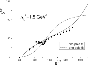
Figure 2: Phase shifts obtained from the fit to LASS data up to 1510MeV, to be compared with the data from Ref. [15]. For $\delta^{1/2}_{0}$, solid line: two–pole fit, dashed line: one pole fit.

The $K^{*}_{0}(1430)$ pole outputs in Eq. (S0.Ex6) should not be taken seriously since the couple channel effects already become important at 1500MeV. We will improve our program by incorporating the inelasticity effects later in this paper. What is really surprising and remarkable here is that outputs in the I=1/2, J=0 channel are affected very little considering the magnificent change of $\chi^{2}_{d.o.f.}$. Furthermore the existence of $\kappa$ can still be verified by eliminating $\kappa$ in the fit, which results in $\chi^{2}_{d.o.f.}=3726/(68-2)$ and $a^{1/2}_{0}=0.008$, which are certainly un-acceptable.

It is also noticed that $a^{3/2}_{0}$ is small and $positive$ when taking $\Lambda_{L}^{2}=1.5$GeV². A careful check reveals that in the I=3/2,J=0 channel the circular cut contributes $positively$ to the scattering length, contrary to what happens in the I=1/2, J=0 channel. It is now clear why in Eq. (S0.Ex4) $\Lambda_{3/2}^{2}$ takes a large value: the left hand cut on the real axis has to take a large cutoff to counteract the positive contribution from the circular cut. Whether a NNLO $\chi$PT calculation to the background contribution can reduce such a large $\Lambda_{3/2}^{2}$ remains open. But from the experience in $\pi\pi$ scatterings one may bet that certain improvement is within expectation. Furthermore the present investigation strongly suggests that the high energy contributions are non-negligible in the exotic channel, irrespective to the fact that it cannot be reliably estimated by $\chi$PT. Before any further progress can be made on the exotic channel it is desirable in the following discussions to proceed along with the philosophy adopted when deriving Eq. (S0.Ex4). That is to think the large $\Lambda_{3/2}^{2}$ provides an effective parametrization and is appropriate to separate the exotic channel contribution from LASS data, since the threshold parameters extracted are in agreement with other theoretical estimates, and especially, the $\kappa$ pole is influenced rather little with respect to the uncertainties in the exotic channel.

The Eq. (S0.Ex4) indicates a $\kappa$ pole mass at about $M_{\kappa}\simeq 700$MeV, $\Gamma_{\kappa}\simeq 600$MeV, which agrees with Ref. [16], and is closer to the recent results from production experiments, [17] comparing with Eq. (48) of Ref. [4]. Also it is not strange that the present results are fully compatible with the results of Eqs. (51), (52) and (54) of Ref. [4] since the latter are obtained by imposing the constraints of scattering lengths from chiral estimates.

In the following we also try to extend the data fit range from 1.43GeV to 2.1GeV. The parametrization of inelasticity plays an important role in the attempt to include the region above the inelastic threshold:

$$\mathrm{Im}_{R}f(s)=-{1\over{2\rho(s)}}\log|S^{phy}(s)|$$

$$=-\frac{1}{4\rho}\log\left[1-4\rho\mathrm{Im}_{R}T+4\rho^{2}|T(s)|^{2}\right]\,$$

$$=-\frac{1}{4\rho}\log\left[1-4\rho(\sum_{n}\rho_{n}|T_{1n}(s)|^{2}+\cdots)\right]\ .$$ (15)

The approximation we adopt for the right hand cut are from Ref. [18]. When third-sheet or higher sheet pole contributions dominate inelasticity, we have[10]

$$T_{1n}=\frac{1}{\sqrt{\rho_{1}(s)\rho_{n}(s)}}\sum_{r}{{\cal M}_{r}(\Gamma_{r1}\Gamma_{rn})^{\frac{1}{2}}\over{\cal M}_{r}^{2}-s-i{\cal M}_{r}\Gamma_{r}}\,,$$ (16)

with $\Gamma_{rn}$ the partial width, $\Gamma_{r}$ the total width.

The $K\pi$ scatterings in both $I=1/2$ and $I=3/2$ channels are inelastic when $K\eta^{\prime}$ channel opens above roughly 1.4 GeV. Actually, a $K_{0}^{*}(1950)$ resonance was observed by LASS experiment [1]. Assuming inelasticity in I=1/2 channel is contributed solely from $K_{0}^{*}(1950)$, the right hand cut integral is evaluated by using Eq. (S0.Ex8) and Eq. (16). As for the I=3/2 channel, it is thought to be elastic below 1.5 GeV according to its small cross section. Above 1.5GeV the phase shift begin to rise slowly according to the analysis given in Ref. [15]. It should be noticed that within the present approximation scheme it is impossible to explain such a rise of phase shift. Because the J=0, I=3/2 channel is exotic and what we have to use in Eq. (16) is the resonance dominance approximation. What we assume here is that the inelasticity in the exotic channel solely comes from the left hand cut approximated by $\chi$PT results and the contribution coming from the right hand cut is negligible. This may be considered as a drawback of the present approach but hopefully its influence to the determination of the $K_{0}(1950)$ pole location is not large.

There are two solutions of data in Ref. [1]. They are the same below 1.8 GeV, but different above 1.8 GeV due to Barrelet ambiguity. The data in the energy region roughly between 1.6 to 1.8 GeV should not be trusted. The reason is very simple,[16]

$$a_{0}e^{i\phi_{0}} = {1\over 4}[(2\eta_{1/2}\sin 2\delta_{1/2}+\eta_{3/2}\sin 2\delta_{3/2})\ ;$$ (17)

$$+ i(3-2\eta_{1/2}\cos 2\delta_{1/2}-\eta_{3/2}\cos 2\delta_{3/2})]$$

where $a_{0}$ and $\phi_{0}$ are the quantities LASS experimental group measured. Unitarity demands that the imaginary part of the $r.h.s.$ of the above equation be positive definite, so it is impossible for $\phi_{0}$ to be larger than $180^{\circ}$. For the same reason, we give up fit to the solution B of Ref. [1].

In the J=0, I=1/2 channel there are contributions from the left hand cut; 3 second sheet poles, $\kappa$, $K^{II}_{0}(1430)$ and one to be determined; two third sheet poles $K_{0}^{III}(1430)$ and $K^{III}_{0}(1950)$ through the right hand cut integrals. The fit results up to 2.1GeV are shown below,

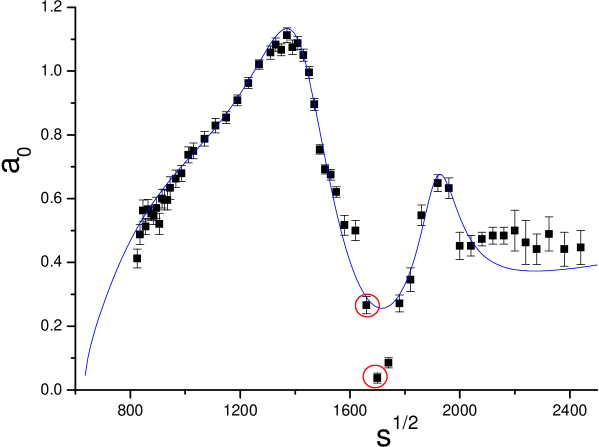
Figure 3: Fit to $a_{0}$ of LASS data up to 2.1GeV (data points encircled violate unitarity and are not used in the fit).

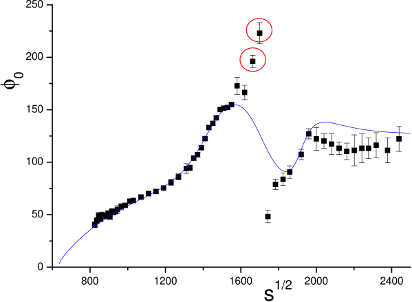
Figure 4: Fit to $\phi_{0}$ of LASS data up to 2.1GeV (data points marked by red circles violate unitarity)

$$\chi^{2}_{d.o.f.}=229.5/(96-14)\ ;$$

$$M_{\kappa}=649\pm 63MeV\ ,\,\,\,\Gamma_{\kappa}=602\pm 22MeV\ ;$$

$$M_{K^{II}_{0}(1430)}=1435\pm 6MeV\ ,\,\,\,\Gamma_{K^{II}_{0}(1430)}=288\pm 22MeV\;$$

$$M_{K_{0}^{*}(1950)}=1917\pm 12MeV\ ,\,\,\,\Gamma_{K_{0}^{*}(1950)}^{tot}=145\pm 38MeV\ ;$$

$$\Gamma_{K_{0}^{*}(1950)}^{K\pi}=87\pm 14MeV\ .$$ (18)

Notice that the encircled data points as depicted in Figs. 2 and 3 are subtracted when making the fit. The threshold parameters are also consistent with the previous results, though $a_{0}^{1/2}$ and $b_{0}^{1/2}$ are increased by roughly 1$\sigma$ error bar. Not listed in above results are $K_{0}^{III}(1430)$ and the additional second sheet pole (which simulates the possible second sheet $K_{0}^{*}(1950)$ pole) except the $\kappa$ and $K_{0}^{II}(1430)$. Because it is found that these two poles (contributing 5 additional parameters together) only reduce the total $\chi^{2}$ roughly by 2, hence their existence is not apparent at all. Without them in the fit only makes tiny changes to other physical outputs. We will discuss again related topics later in this paper. Before that we want to check the cutoff dependence of the above outputs. If fixing the two cutoff parameters at for example $\Lambda_{L}^{2}=1.5$GeV² and let other conditions being the same as in deriving Eq. (S0.Ex11), then one finds $\chi^{2}_{d.o.f.}=777/(96-12)$, and the $\kappa$ pole’s mass and width are both further decreased by roughly 100MeV comparing with Eq. (S0.Ex11) but with ridiculously small error bars. Hence the results are un-trustworthy. For the case without $\kappa$ the output is rather similar at low energies to the situation of the one pole fit as depicted by Fig. 2, which is apparently un-physical.

The $\kappa$ resonance pole position determined in Eq. (S0.Ex11) agrees within 1$\sigma$ with that of Eq. (S0.Ex4). The third sheet $K_{0}^{*}(1950)$’s mass, total width and its partial decay width into $K\pi$ are found in good agreement with the results obtained by the LASS Collaboration [1] and that of Anisovich and Sarentsev [19]. The major difference between Eq. (S0.Ex11) and Eq. (S0.Ex4) is the decay width of $K^{{II}}_{0}(1430)$. In Eq. (S0.Ex4) the $K^{{II}}_{0}(1430)$ pole is determined by fitting data only up to 1430MeV and hence the outputs on $K^{{II}}_{0}(1430)$ parameters given by Eq. (S0.Ex11) may be more preferable. Furthermore, unlike the situation of $f_{2}(1270)$ [8] where the twin pole structure of $f_{2}(1270)$ is clearly identified, here we are lacking of the separate data of the inelasticity parameter in the I=1/2 channel. Hence the observation on the absence of $K^{III}_{0}(1430)$ from the analysis in Eq. (S0.Ex11) only provides a possibility, but not a definite conclusion. On the other side, the analysis on the unitarized scattering amplitudes from resonance chiral lagrangian model do generate a typical couple channel Breit–Wigner resonance structure for $K_{0}^{*}(1430)$. [16] The PKU parametrization form, which makes clear distinction between the second sheet pole and the third sheet pole, is more sensitive to the second sheet pole rather than the third sheet pole in the absence of the data of inelasticity parameter. Different from the $K_{0}^{*}(1430)$ pole, for the $K_{0}(1950)$ resonance on the third sheet, our analysis definitely confirms its existence. However, in disagreement with Ref. [16], we did $not$ find evidences in support of its counterpart on the second sheet. A narrow second sheet pole around 1950MeV, according to Eq. (1), will provide a rapid phase motion for $\delta$ and also for $\phi_{0}$ around 1950MeV. Nevertheless it is seen from fig. 4 that the major part of the enhancement of $\phi_{0}$ around 1950MeV may already be explained by $K^{III}_{0}(1950)$ combined with other background contributions. If our observation is correct it would suggest that the $K_{0}^{*}(1950)$ may not be a typical Breit–Wigner resonance. But of course, more careful analysis on more accurate data is needed to clarify this issue.

The stability of our fit results on the 3rd sheet $K_{0}^{*}(1950)$ pole can be further investigated. In getting Eq. (S0.Ex11) the fit is performed up to 2.1GeV. The effects from possible higher resonances were not considered. In order to check the stability of the results we also made the fit up to 2.5GeV using the same parameter set as Eq. (S0.Ex11) is obtained, and bare in mind that the two additional 2nd sheet and 3rd sheet poles now may effectively simulate effects from higher energies. Indeed, the fit indicates these additional poles now locate at around 3GeV with sizable error bars. Of course these additional outputs themselves are of no value to mention. The major concern is the stability of the $K_{0}^{*}(1950)$ pole. It turns out that the rest of the fit results are very similar to that of Eq. (S0.Ex11) except that the total width of the 3rd sheet $K_{0}^{*}(1950)$ pole is now reduced by less than 20MeV (with the branching ratio almost unchanged). Such a reduction in total width is acceptable since it’s within the error as given in Eq. (S0.Ex11).

To conclude, comparing with Ref. [4] the correct use of analyticity led us to have stronger confidence on the existence of the $\kappa$ resonance, based on the LASS data. Scattering length parameters are also found to be, naturally, in agreement with chiral theory results. The pole mass and width for the low lying $\kappa$ resonance are found to be $M_{\kappa}=694\pm 53MeV$, $\Gamma_{\kappa}=606\pm 59MeV$, respectively. The $K_{0}^{*}(1430)$ and $K_{0}^{*}(1950)$ resonances are also studied by fitting the LASS data up to 2.1GeV and the result is given in Eq. (S0.Ex11). Finally, according to the LASS data we did not find it necessary to introduce the $K_{0}^{*}(1430)$ pole on the third sheet and the $K_{0}^{*}(1950)$ pole on the second sheet, since they do not contribute to the decreasing of total $\chi^{2}$.

In recent few years considerable progresses have been made in studying the low lying scalar resonances in hadron spectrum. For the $\sigma$ meson, it is demonstrated that the $\sigma$ is crucial for chiral perturbation theory to accommodate for the CERN–Munich I,J=0,0 $\pi\pi$ scattering phase sheet data. [11] A rather precise determination to the $\sigma$ pole location can be obtained. [20, 8] The situation for the $\kappa$ resonance is less clear, due to the flawed data as well as that crossing symmetry is not yet used in the determination of the $\kappa$ pole. Though the current study confirms the existence of the $\kappa$ resonance, more efforts have to be made in order to get a precise understanding to the $\kappa$ pole location.

Acknowledgement: We thank one referee’s stimulating remarks which are helpful in formulating the discussions in its present form. This work is support in part by National Nature Science Foundations of China under contract number 10575002,10421503and 10491306.

Appendix

Here we present the proof of the statement that if the full scattering amplitude is polynomial bounded then $f(0)=0$. In order to achieve this, according to the previous text in this paper, one only needs to prove $T^{I}_{J}(s\to 0)$ is no more singular than $O(s^{-n})$ where $n$ is an arbitrary but finite constant.

The proof can be made following the method of Ref. [9], but in the present case the situation is simpler. From partial wave projection formula,

$$T^{I}_{J}(s) = {1\over 32\pi}{1\over 2{q_{s}}^{2}}\int_{-4{q_{s}}^{2}}^{0}dtP_{J}(1+{{t}\over{2{q_{s}}^{2}}})T^{I}(s,t,u)\ ,$$ (19)

and Eq. (S0.Ex2) we see that,

$$q_{s}^{2}\to\frac{(m_{K}^{2}-m_{\pi}^{2})^{2}}{4}s^{-1}\to+\infty\,\,\,\,\,(\mbox{when}\,\,\,s\to 0_{+})\ .$$ (20)

Hence the asymptotic limit of $T^{I}_{J}(s)$ when $s\to 0_{+}$ is governed by the asymptotic behavior of $T^{I}(s,t)$ when $s\to 0_{+}$ and $t\to-\infty$, through Eq. (19). On the other side, the asymptotic behavior of $T(s\to 0_{-})$ is governed by the asymptotic behavior of $T^{I}(s,t)$ when $s\to 0_{-}$ and $t\to+\infty$. The physical region of $\pi K\to\pi K$ is given by $t=0$ and the hyperbola $su=(m_{K}^{2}-m_{\pi}^{2})$. The boundaries of the double spectral regions can be found in, for example, Ref. [21]. It is noticed that $T^{I}(s,t)$ is a regular function of $s$ at $s=0$ for any fixed $t$, since on the Mandelstam plot the line $s=0$ does not touch any of the double spectral region. Hence we only need to discuss the $t\to\pm\infty$ limit of $T^{I}(s,t)$ for fixed small positive $s$. In such a situation, one can prove the following relation,

$$\lim_{t\to+\infty}T^{I}(s,t)=\lim_{t\to-\infty}T^{I}(s,t)\$$ (21)

using a mathematical theorem which states that: a function which is analytic in the upper half of the complex $z$ plane and does not increase exponentially for $|z|\to\infty$ along any ray in the upper half of $z$ plane, cannot tend to different limits along the positive and negative real axis (of course only along the upper edge). The conditions for this theorem to hold are no more than the Mandelstam analyticity assumption.

Therefore we consider the $s\to 0_{+}$ limit of Eq. (19), taking $J=0$ only for simplicity. Assuming $|T(s,t)|<|t|^{n}$ for any fixed $s$ and large $|t|$, we have

$$\lim_{s\to+0}|T^{I}_{0}(s)| < \lim_{s\to 0_{+}}{1\over 32\pi}{1\over 2{q_{s}}^{2}}\int_{-4{q_{s}}^{2}}^{0}dt|T^{I}(s,t)|$$ (22)

$$< \lim_{s\to 0_{+}}{1\over 32\pi}{1\over 2{q_{s}}^{2}}\int_{-4{q_{s}}^{2}}^{0}dt|t|^{n}$$

$$\sim O(s^{-n})\ .$$

Hence we complete the proof.

If higher partial waves are considered, each term of the Legendre polynomial in Eq. (19) contributes at the same order when $s\to 0$ and the sum results only in an additional coefficient in front of $O(s^{-n})$. See Ref. [9] for details.

References

- [1] D. Aston (LASS Collaboration), Nucl. Phys. B296(1988)493.
- [2] Here we are only able to provide a few previous publications on this issue: E. van Beveren , Z. Phys. C30(1986)615; N. A. Tornqvist, Z. Phys. C68(1995)647; S. Ishida , Prog. Theor. Phys. 98(1997)621; D. Black , Phys. Rev. D58(1998)054012. F. K. Guo , hep-ph/0509050.
- [3] S. N. Cherry and M. R. Pennington, Nucl. Phys. A688(2001)823.
- [4] H. Q. Zheng , Nucl. Phys. A733(2004)235.
- [5] V. Bernard, N. Kaiser and Ulf-G. Meissner, Nucl. Phys. B357(1991)129.
- [6] Similar opinion is also emphasized by David Bugg: private communications.
- [7] J. Kennedy and T. D Spearman, Phys. Rev. 126(1962)1956.
- [8] Z. Y. Zhou et al., JHEP0502(2005)043.
- [9] H.-P. Jakob and F. Steiner, Z. Physik 228(1969)353.
- [10] P. D. B. Collins, An Introduction to Regge Theory and High Energy Physics, Cambridge University Press, 1977.
- [11] Z. G. Xiao and H. Q. Zheng, Nucl. Phys. A695(2001)273; Z. G. Xiao and H. Q. Zheng, talk given at International Conference on Flavor Physics (ICFP 2001), Zhang-Jia-Jie City, Hunan, China, 31 May - 6 Jun 2001, hep-ph/0107188.
- [12] J. Y. He, Z. G. Xiao and H. Q. Zheng, Phys. Lett. B536(2002)59; Erratum-ibid. B549(2002)362.
- [13] P. Büttiker, S. Descotes-Genon and B. Moussallam, Eur. Phys. J. C33(2004)409.
- [14] M. Krivoruchenko, Z. Phys. A350(1995)343.
- [15] P. Estabrooks , Nucl. Phys. B133(1978)490.
- [16] M. Jamin, J. A. Oller and A. Pich, Nucl. Phys. B587(2000)331.
- [17] M. Ablikim et al. (BES Collaboration), Phys. Lett. B633(2006)681; D. Bugg, Eur. Phys. J. A25(2005)107, Erratum-ibid. A26(2005)151; E. M. Aitala et al. (E791 Collaboration), Phys. Rev. Lett. 89(2002)121801.
- [18] J. J. Wang, Z. Y. Zhou and H. Q. Zheng, JHEP 0512(2005)019.
- [19] A. V. Anisovich and A. V. Sarantsev, Phys. Lett. B413(1997)137.
- [20] I. Caprini, G. Colangelo and H. Leutwyler, Phys. Rev. Lett. 96(2006)132001.
- [21] C. B. Lang, Fortschritte der Physik, 26(1978)509.