Yukawa and Tri-scalar Processes
in Electroweak Baryogenesis

Abstract

We derive the contributions to the quantum transport equations for electroweak baryogenesis due to decays and inverse decays induced by tri-scalar and Yukawa interactions. In the Minimal Supersymmetric Standard Model (MSSM), these contributions give rise to couplings between Higgs and fermion supermultiplet densities, thereby communicating the effects of CP-violation in the Higgs sector to the baryon sector. We show that the decay and inverse decay-induced contributions that arise at zeroth order in the strong coupling, $\alpha_{s}$, can be substantially larger than the ${\cal O}(\alpha_{s})$ terms that are generated by scattering processes and that are usually assumed to dominate. We revisit the often-used approximation of fast Yukawa-induced processes and show that for realistic parameter choices it is not justified. We solve the resulting quantum transport equations numerically with special attention to the impact of Yukawa rates and study the dependence of the baryon-to-entropy ratio $Y_{B}$ on MSSM parameters.

I Introduction

The origin of the baryon asymmetry of the universe (BAU) remains an open question for particle physics, nuclear physics, and cosmology. Although the size of the BAU cannot be explained within the framework of the Standard Model (SM), there exist a variety of SM extensions that may allow for successful baryogenesis. Scenarios in which the BAU is produced at the electroweak phase transition are particularly attractive since they can be tested with laboratory experiments. To the extent that the masses of the particles responsible for baryogenesis are not too different from the weak scale, their dynamics can be studied using a combination of collider experiments, precision electroweak measurements, and CP-violation studies.

In order to carry out robust tests of electroweak baryogenesis (EWB), it is necessary to delineate systematically the quantitative relationship between EWB and experimentally accessible observables. The motivation for doing so has been heightened by the prospect of significant new experimental information in the near term. Studies at the Large Hadron Collider will search for the existence of new particles at the TeV scale. At the same time, a new generation of searches for permanent electric dipole moments of the electron, neutron, and neutral atoms will look for the effects of “new” CP-violation with several orders of magnitude better sensitivity than given by current experimental limits (see, e.g., Refs. Erler:2004cx ; Pospelov:2005pr and references therein). Should either the LHC or EDM searches discover evidence for new physics at the electroweak scale, then precision studies at both the International Linear Collider and low-energy facilities should provide detailed information about the structure of the new physics. To the extent that the theoretical treatment of EWB is on sufficiently firm ground, these experimental efforts may either confirm or rule out this paradigm for the BAU.

The basic physical picture of EWB was developed over a decade ago Cohen:1994ss ; HN ; Joyce:1994fu ; Joyce:1994zn (see Trodden:1998ym for a review). The elements include a first-order electroweak phase transition, in which bubbles of broken electroweak symmetry expand and fill the universe as it cools through the transition temperature. CP- and C-violating interactions between fields in the plasma at the phase boundary create a net chiral charge that is injected into the region of unbroken electroweak symmetry, driving the weak sphaleron processes that create non-zero baryon number density, $n_{B}$. The expanding bubbles then capture the non-zero $n_{B}$ in the region of broken electroweak symmetry, where weak sphaleron processes are highly suppressed and unable to affect $n_{B}$ appreciably. It is crucial that the first-order phase transition be sufficiently strong in order to preclude “wash out” of non-zero baryon number.

The earliest analyses based on this picture employed conventional transport theory to compute the production, diffusion, and relaxation of chiral charge at the phase boundary. Several groups have subsequently endeavored to put these computations on a more sophisticated footing by using non-equilibrium quantum field theory techniques. As first pointed out by Riotto riotto0 ; riotto , only a non-equilibrium field-theoretic formulation can properly account for the quantum nature of CP violation as well as the decoherence effects due to the presence of spacetime-varying background fields and the thermal bath of particles at the phase boundary. Using these methods Riotto riotto observed that conventional treatments may overlook significant enhancement of the CP-violating source terms in the transport equations associated with memory effects in the plasma. The presence of such enhancements could relax the requirements on new CP-violation needed for successful EWB, thereby allowing for consistency between the BAU and considerably smaller EDMs than previously thought. This work was followed by the authors of Refs. Carena:2000id ; Carena:2002ss , who adopted a similar approach to that of Ref. riotto in computing the CP-violating source terms while carrying out a more comprehensive phenomenology. The analyses of both groups were performed within the Minimal Supersymmetric Standard Model (MSSM). The non-equilibrium approach has also been pursued in Refs. Konstandin:2004gy ; Konstandin:2003dx ; Konstandin:2005cd .

Recently, we investigated the CP-conserving terms as well as the CP-violating sources in the transport equations using non-equilibrium field theory methods us . We found that there exists a hierarchy of physical scales associated with the electroweak phase transition dynamics that allows one to derive the transport equations from the Closed Time Path Schwinger-Dyson equations using a systematic expansion in scale ratios. Again in the MSSM, we computed the CP-violating sources and leading CP-conserving chiral relaxation terms associated with interactions of fermion and Higgs superfields with the spacetime-varying Higgs vacuum expectation values (vevs). Our results for the sources were consistent with those obtained in previous work Carena:1997gx ; riotto ; Carena:2000id ; Carena:2002ss ; Balazs:2004ae , but we also found that enhancements in the relaxation rates could mitigate the effect of enhancements in the sources.

A number of other contributions to the transport equations remain to be analyzed using non-equilibrium methods. Here, we focus on terms that link the dynamics of the quark supermultiplets with those of the Higgs scalars and their Higgsino superpartners. Importantly, these terms are responsible for communicating CP-violating effects in the Higgs supermultiplet densities to the quark supermultiplet densities, thereby allowing CP-violating interactions in the Higgs sector to contribute to baryogenesis. In the MSSM, the requirement of a strong first-order phase transition (shown in Laine to occur in the presence of a light right-handed stop) and constraints from precision electroweak data (requiring the left-handed stop to be heavy Carena:2000id ) imply that it is the CP-violating interactions of the Higgs superfields – rather than those directly involving the squarks – that drives baryogenesis via this coupling between the two sectors. In extensions of the MSSM, such as the NMSSM or U(1)^′ models, the phenomenological requirements that preclude large effects from CP-violation in the squark sector can be relaxed nonminimal , and in this case it is important to know the relative importance of Higgs sector CP-violation. In either case, an analysis of the dynamics whereby the baryon and Higgs sectors communicate is an important component of a systematic, quantitative treatment of EWB.

Before providing the details of our study, we summarize the primary results, using the transport equation for the Higgs $+$ Higgsino densities for illustration:

$$\partial^{\mu}H_{\mu}=-\Gamma_{H}\frac{H}{k_{H}}-\Gamma_{Y}\biggl{(}\frac{Q}{k_{Q}}-\frac{T}{k_{T}}+\frac{H}{k_{H}}\biggr{)}-{\tilde{\Gamma}}_{Y}\biggl{(}\frac{B}{k_{B}}-\frac{Q}{k_{Q}}+\frac{H}{k_{H}}\biggr{)}+\bar{\Gamma}_{Y}\frac{h}{k_{h}}+S_{\tilde{H}}^{CP\!\!\!\!\!\!\!\!\raisebox{0.0pt}{\small$\diagup$}}\ \ \ .$$ (1)

Here, $H$ and $h$ are number densities associated various combinations of the up- and down-type Higgs supermultiplets in the MSSM (defined below); $H_{\mu}$ is the corresponding vector current density; $Q$ and ($B$,$T$) are the number densities of particles in the third generation left- and right-handed quark supermultiplets, respectively; the $k_{H,h,Q,T,B}$ are statistical weights; $S_{\tilde{H}}^{CP\!\!\!\!\!\!\!\!\raisebox{0.0pt}{\small$\diagup$}}$ is a CP-violating source; and $\Gamma_{H}$, $\Gamma_{Y}$, ${\tilde{\Gamma}}_{Y}$, and $\bar{\Gamma}_{Y}$ are transport coefficients.

Physically, the presence of $S_{\tilde{H}}^{CP\!\!\!\!\!\!\!\!\raisebox{0.0pt}{\small$\diagup$}}$ results from an imbalance between the rates for particle and antiparticle scattering off the bubble wall, favoring the generation of non-vanishing supermultiplet densities $H$ and $h$. In contrast, the terms proportional to $\Gamma_{H}$ and $\bar{\Gamma}_{Y}$ cause these densities to relax to zero. The terms containing $\Gamma_{Y}$ and ${\tilde{\Gamma}}_{Y}$ favor chemical equilibrium between Higgs superfield densities and those associated with quark supermultiplets. To the extent that the rates $\Gamma_{Y}$ and ${\tilde{\Gamma}}_{Y}$ are fast compared to the rate of relaxation, any non-vanishing Higgs supermultiplet density quickly induces non-vanishing densities for quark supermultiplets, thereby facilitating EWB. Understanding the microscopic dynamics of this competition between CP-violating sources, relaxation terms, and Higgs-baryon sector couplings is essential to achieving a quantitative description of EWB.

In previous work, we computed $\Gamma_{H}$ and $S_{\tilde{H}}^{CP\!\!\!\!\!\!\!\!\raisebox{0.0pt}{\small$\diagup$}}$ using the Closed Time Path Schwinger-Dyson equations and considering the lowest-order couplings between superfields and the spacetime varying Higgs vevs. Here, we focus on the terms proportional to $\Gamma_{Y}$, $\bar{\Gamma}_{Y}$, $\tilde{\Gamma}_{Y}$ that are generated by $Hqq$ Yukawa couplings, the corresponding supersymmetric interactions, and the SUSY-breaking triscalar couplings. We make several observations regarding these terms:

• In previous treatments, $\Gamma_{Y}$ and ${\bar{\Gamma}}_{Y}$ were estimated from scattering processes such as $t_{R}+g\to t_{L}+H_{u}^{0}$, making them proportional to one power of the strong coupling, $\alpha_{s}$. We find, however, that there exist contributions to $\Gamma_{Y}$ occurring at zeroth order in $\alpha_{s}$ that are generated by decay and inverse decay processes such as $t_{R}+t_{L}\leftrightarrow H_{u}^{0}$. To the extent that the three-body processes are kinematically allowed, their contribution to $\Gamma_{Y}$ can be considerably larger than those generated by scattering. We also show that $|{\bar{\Gamma}}_{Y}/\Gamma_{Y}|$ is typically $<1/2$ for MSSM parameters consistent with precision electroweak data and the existence of a strong first order phase transition. (The authors of Ref. Carena:2000id argued that $|{\bar{\Gamma}}_{Y}|=|\Gamma_{Y}|$.) We solve the transport equations numerically and find that inclusion of the three-body contributions affects the baryon-to-entropy ratio $Y_{B}$ at the $10-20\%$ level for realistic choices of the MSSM parameters. We provide a detailed analysis of the dependence of $Y_{B}$ on $\Gamma_{Y}$ and the MSSM parameters that determine it.

• In most of the early studies of EWB in the MSSM, it was assumed that the rate $\Gamma_{Y}$ of Yukawa-induced processes is “fast” compared to all other relevant time-scales, implying that the Yukawa-induced transfer of non-zero Higgs/Higgsino density to non-vanishing chiral charge density is more efficient than relaxation. This assumption has motivated an expansion in powers of $1/\Gamma_{Y}$. We show that there exist corrections to the Higgs density at linear order in this expansion that have not been included in previous treatments. After including these terms, we find that the expansion itself breaks down – even for the enhanced values of $\Gamma_{Y}$ that result from inclusion of the three-body contributions – due to the presence of chirality-changing processes in the bubble wall whose rates $\Gamma_{H}$ and $\Gamma_{M}$ can be larger than $\Gamma_{Y}$. We study numerically the impact of keeping a finite $\Gamma_{Y}$: we find that the corrections to the $\Gamma_{Y}\to\infty$ limit of $Y_{B}$ range between $20\%$ and $100\%$, depending on the values of the other rates.

• The terms containing $\Gamma_{Y}$ and $\bar{\Gamma}_{Y}$ have been included in the earlier studies of Refs. Cline:2000kb ; Cline:2000nw ; Carena:2000id ; Carena:2002ss , whereas the one involving $\tilde{\Gamma}_{Y}$ is new. In the MSSM, one often assumes that the triscalar coupling involving the down-type Higgs scalars, the doublet scalars ${\tilde{Q}}$, and the right handed scalars $\tilde{b}$ is proportional to the bottom Yukawa coupling, $y_{b}$. For $\tan\beta\sim{\cal O}(1)$, one has $y_{b}/y_{t}\ll 1$ and the impact of the $\tilde{\Gamma}_{Y}$ term is relatively minor. For scenarios with large $\tan\beta$, however, $y_{b}$ need not be small compared to $y_{t}$. In this case the transport coefficient ${\tilde{\Gamma}}_{Y}$ and other terms (not shown) that couple to the $B$ supermultiplet need not be suppressed, and the coupled set of transport equations must be augmented to include dynamical $b$-quarks and their superpartners. Although in the present study we do not consider this large $\tan\beta$ scenario, we provide the general formulas that allow one compute ${\tilde{\Gamma}}_{Y}$.

In the remainder of the paper, we discuss our detailed analysis of the $\Gamma_{Y}$-type terms that lead to these observations. In Section II, we consider these terms for generic Yukawa and tri-scalar interactions and analyze their dependence on the relevant mass parameters. In Section III we specify to the MSSM, including detailed analytic and numerical studies. Here, we include contributions from both SM particles and their superpartners (in contrast to previous anlayses that included only SM scattering terms), and note that the superpartner contributions tend to increase the magnitude of $\Gamma_{Y}$. In Section IV we solve the coupled transport equations to obtain the baryon-to-entropy ratio, and show why one would not expect an expansion in $1/\Gamma_{Y}$ to yield a reasonable approximation to the exact solution. We summarize this work in Section V. Various technical points are discussed in the Appendices.

II Three-body source terms: building blocks

Our approach for deriving the source terms in the quantum transport equations is based on the Closed Time Path Schwinger-Dyson equations. An extensive discussion of this framework is given in our earlier work us . Here, we give a brief summary of our method and use it to derive the source terms generated by supersymmetric Yukawa and SUSY-breaking tri-scalar interactions to leading order in the loop expansion.

II.1 Formalism and method

Ordinary quantum field theory is not appropriate for treating the microscopic dynamics of the electroweak phase transition (EWPT), since the non-adiabatic evolution of states and the presence of degeneracies in the spectrum break the zero-temperature, equilibrium relation between the in- and out-states. The non-adiabaticity arises because particle interactions occur against a spacetime-varying background field (the Higgs vevs), while thermal effects associated with non-zero temperature introduce degeneracies in the spectrum. The impact of non-adiabaticity and degeneracies on quantum evolution can be treated systematically using the Closed Time Path (CTP) formalism CTP . In this formulation the time arguments of all fields and composite operators lie on a path ${\cal P}$ that consists of a positive branch ${\cal P}_{+}$ from $-\infty$ to $+\infty$ and a negative branch ${\cal P}_{-}$ running back from $+\infty$ to $-\infty$. Fields whose arguments lie on ${\cal P}_{+}$ precede those on ${\cal P}_{-}$ along the path ${\cal P}$. Moreover, those lying on ${\cal P}_{+}$ are time-ordered while those on ${\cal P}_{-}$ are anti-time-ordered.

With this prescription the standard time-ordering operator $T$ is replaced by the path-ordering operator $T_{\cal P}$ and the perturbative expansion is formally identical to the equilibrium case. In applying Wick’s theorem, however, one must allow for contractions involving all possible combinations of fields taken from either ${\cal P}_{+}$ and ${\cal P}_{-}$, leading to a generalized Green’s function that accounts for path-ordering. Specifically, the bosonic and fermionic Green functions are given by

$$G(x,y) = \langle T_{\cal P}\,\left[\phi(x)\phi^{\dagger}(y)\right]\rangle$$ (2)

$$S(x,y) = \langle T_{\cal P}\,\left[\psi(x)\overline{\psi}(y)\right]\rangle$$ (3)

where $\langle...\rangle$ denotes an average over the physical state of the system, which may be described by an appropriate density matrix. In practical applications it is convenient to use ordinary time arguments, in terms of which each of Eq. (2) and (3) represents four Green functions and decomposes in various components. To establish the notation we recall here explicitly the bosonic Green functions:

$$G^{++}(x,y) \equiv G^{t}(x,y)=\langle T\,\left[\phi(x)\phi^{\dagger}(y)\right]\rangle$$ (4)

$$G^{+-}(x,y) \equiv G^{<}(x,y)=\langle\phi^{\dagger}(y)\phi(x)\rangle$$ (5)

$$G^{-+}(x,y) \equiv G^{>}(x,y)=\langle\phi(x)\phi^{\dagger}(y)\rangle$$ (6)

$$G^{--}(x,y) \equiv G^{\bar{t}}(x,y)=\langle\bar{T}\,\left[\phi(x)\phi^{\dagger}(y)\right]\rangle\ \ \ ,$$ (7)

where the superscripts “$a$” and “$b$” in $G^{ab}(x,y)$ indicate the branch ${\cal P}_{\pm}$ on which the time components of $x$ and $y$ lie, respectively and where ${\bar{T}}$ is the anti-time-ordering operator.

The equations governing the spacetime dependence of number densities of a given bosonic or fermionic species can be derived from the Schwinger-Dyson equations for the generalized Green’s functions $G(x,y)$ and $S(x,y)$ and have the following form kadanoff-baym ; riotto :

$$\begin{split}\frac{\partial n_{B}}{\partial X_{0}}(X)+{\mbox{\boldmath$\nabla$}}\!\cdot\!\mathbf{j}_{B}(X)=\int d^{3}z\int_{-\infty}^{X_{0}}dz_{0}\ \Bigl{[}\Sigma_{B}^{>}(X,z)G^{<}(z,X)&-G^{>}(X,z)\Sigma_{B}^{<}(z,X)\\ +G^{<}(X,z)\Sigma_{B}^{>}(z,X)&-\Sigma_{B}^{<}(X,z)G^{>}(z,X)\Bigr{]}\,.\end{split}$$ (8)

$$\begin{split}\frac{\partial n_{F}}{\partial X_{0}}(X)+{\mbox{\boldmath$\nabla$}}\!\cdot\!\mathbf{j}_{F}(X)=-\int d^{3}z\int_{-\infty}^{X_{0}}dz_{0}\ {\rm Tr}\Bigl{[}\Sigma_{F}^{>}(X,z)S^{<}(z,X)&-S^{>}(X,z)\Sigma_{F}^{<}(z,X)\\ +S^{<}(X,z)\Sigma_{F}^{>}(z,X)&-\Sigma_{F}^{<}(X,z)S^{>}(z,X)\Bigr{]}\,.\end{split}$$ (9)

The RHS involves a causal time integral over the system’s history and is expressed in terms of the Green functions (2), (3) and self energies $\Sigma_{B,F}$ that encode all the information about particle interactions. This feature allows for a consistent treatment of both CP-violating terms “sourcing” a given particle density as well as CP-conserving interactions that tend to transfer this density to other species or cause it to relax away. Previously, the leading CP-violating contributions to $\Sigma_{B,F}$ generated by scattering from the Higgs vevs (see Fig. 1) were computed in Refs. riotto ; Carena:2002ss ; Carena:2000id ; Balazs:2004ae ; us while the corresponding CP-conserving relaxation terms generated by the same processes were derived in Ref. us . Here, we extend these analyses to include the three-body source terms that arise from Yukawa and tri-scalar interactions at one-loop order (see Fig. 2).

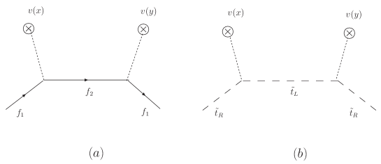
Figure 1: Leading contributions to the self-energies $\Sigma_{B,F}$ generated by scattering from Higgs vevs.

In general, the Green’s functions (2), (3) are dynamical objects that can be obtained by solving the transport equations (8) and (9). However, the hierarchy of time and energy scales present during the electroweak phase transition allow for simplifications in treating the transport equations us . The time scales are a decoherence time, $\tau_{\rm d}$, associated with the departure from adiabatic evolution; a “plasma” time, $\tau_{\rm p}$, associated with mixing between degenerate states in the finite temperature spectrum; and the “intrinsic” quasiparticle evolution time, $\tau_{\rm int}$, associated with time evolution of a state of definite energy. In terms of physical parameters associated with the plasma, one has $\tau_{\rm d}\sim 1/(v_{w}k_{\rm eff})$, $\tau_{\rm p}\sim 1/\Gamma_{p}$, and $\tau_{\rm int}\sim 1/\omega$, where $v_{w}$ is the velocity of expansion of the bubble wall; $k_{\rm eff}$ is an effective wave number that in general depends on the quasiparticle wave number and wall thickness, $L_{w}$; $\Gamma_{p}$ is the thermal width of the quasiparticle; and $\omega$ is the quasiparticle frequency that depends on both the particle momentum and thermal mass. For the EWPT, one has that $\varepsilon_{\rm d}=\tau_{\rm int}/\tau_{\rm d}\ll 1$; $\varepsilon_{\rm p}=\tau_{\rm int}/\tau_{\rm p}\ll 1$; and $\varepsilon_{\rm d}/\varepsilon_{\rm p}=\tau_{\rm p}/\tau_{\rm d}\ll 1$. In addition, the small densities present at the EWPT imply a hierarchy of energy scales: $\varepsilon_{\mu}=\mu/T\ll 1$, where $\mu$ refers to the chemical potential of any particle species. The existence of these hierarchies allows for a number of simplifying approximations in solving the transport equations:

• Use of the quasiparticle ansatz for the $G_{i}(x,y)$. This relies on $\varepsilon_{\rm p}\ll 1$, that is, that the damping rates $\Gamma_{p}$ that broaden the spectrum of excitations are typically suppressed when compared with the excitation frequencies ($\Gamma_{i}/\omega_{i}\ll 1$).

• Working near kinetic and chemical equilibrium. This approximation relies on $\tau_{\rm p}/\tau_{\rm d}\ll 1$, that is, the plasma interactions among quasiparticles are fast compared to the decoherence time, thereby leading to approximate, local equilibrium among quasiparticle species. Consequently, one may approximate quasiparticle distribution functions appearing in the Green functions by their equilibrium forms and track quasiparticle densities with local chemical potentials. The error engendered by doing so is ${\cal O}(\varepsilon_{\rm d}/\varepsilon_{\rm p})$ and is, thus, negligible.

Motivated by these considerations we evaluate the source terms on the RHS of the transport equations (8) and (9) using the free-particle form of the Green functions. For example, for the boson Green functions, we have

$$G_{i}^{>}(x,y) = \int\frac{d^{4}k}{(2\pi)^{4}}e^{-ik\cdot(x-y)}\Bigl{[}1+f_{B}(k_{0},\mu_{i})\Bigr{]}\ \rho_{i}(k_{0},{\bf k})$$ (10)

$$G_{i}^{<}(x,y) = \int\frac{d^{4}k}{(2\pi)^{4}}e^{-ik\cdot(x-y)}f_{B}(k_{0},\mu_{i})\ \rho_{i}(k_{0},{\bf k})$$ (11)

with spectral functions $\rho_{i}(k_{0},{\bf k})=\pi/\omega_{\bf k}\left[\delta(k^{0}-\omega_{\bf k})-\delta(k^{0}+\omega_{\bf k})\right]$ ($\omega_{\bf k}=\sqrt{{\bf k}^{2}+m^{2}}$) that can be appropriately modified to take into account collision-broadening and thermal masses, and distribution functions close to the equilibrium form

$$f_{B}(k_{0},\mu_{i})=n_{B}(k_{0},\mu_{i})+{\cal O}(\varepsilon_{\rm d}/\varepsilon_{\rm p})\ \ \ ,$$ (12)

where $n_{B}(k_{0},\mu_{i})=1/[e^{(k_{0}-\mu_{i})/T}-1]$ and $\mu_{i}$ is a local chemical potential .

Upon expanding the source terms to lowest non-trivial order in the $\varepsilon_{{\rm d},{\rm p},\mu}$ and relating current and chemical potential to local densities through

$${\bf j}_{i}(X)=-D_{i}\,\nabla n_{i}(X)\qquad\qquad n_{i}(X)=\frac{T^{2}}{6}\,k_{i}(m_{i}/T)\,\mu_{i}(X),$$ (13)

where $k_{i}(m_{i}/T)$ is a statistical factor (see, e.g. us ), we obtain the quantum transport equations

$$\dot{n}_{i}-D_{i}\nabla^{2}n_{i}=S_{i}[\{n_{j}\}]\ .$$ (14)

In Eq. (14) both CP-violating effects and relaxation rates are encoded in the quantum mechanical sources $S_{i}[\{n_{j}\}]$.

II.2 Results for generic tri-scalar and supersymmetric Yukawa interactions

Let us consider now the generic three-scalar interaction,

$$\mathcal{L}_{\text{int}}=\lambda_{s}A_{s}\phi_{L}\phi_{R}^{*}\phi_{H}+\text{h.c.}\,,$$ (15)

where $\lambda_{s}$ is a dimensionless coupling and $A_{s}$ is a mass scale. This interaction generates contributions to the self-energy appearing on the RHS of Eq. (8) through the one-loop diagram depicted in Fig. 2(c). As an example, we give the self-energy for the complex scalar $\phi_{R}$,

$$\Sigma_{R}^{>,<}(x,y)=-|\lambda_{s}A_{s}|^{2}\,G_{L}^{>,<}(x,y)\,G_{H}^{>,<}(x,y)\ ,$$ (16)

Importantly, the RHS of Eq. (16) is manifestly independent of possible CP-violating phases appearing in the coupling $\lambda_{s}A_{s}$ and therefore does not contribute to the CP-violating source. We obtain similar results for the self-energies of $\phi_{L}$ and $\phi_{H}$. This situation contrasts with that for the Higgs vev scattering contributions derived from Fig. 1, where interference terms involving the up- and down-type Higgs vevs at the different vertices contain CP-violating phase effects.

Inserting Eq. (16) into Eq. (8), using the Green Functions of Eqs. (10,11,12), and expanding to first order in $\varepsilon_{\mu}$ and zeroth order in $\varepsilon_{\rm d,p}$ (setting the thermal widths to zero), we obtain the leading, three-body contribution to $S_{R}$ on the RHS of Eq. (14). We find that the three-body sources for the particle number densities of the complex scalars $\phi_{L}$, $\phi_{R}$ and $\phi_{H}$ are related to each other and are given by

$$\begin{split}S_{R}(X)&=-S_{L}(X)=-S_{H}(X)\\ &=-\left(\mu_{R}-\mu_{L}-\mu_{H}\right)(X)\ \left\lvert\lambda_{s}\right\rvert^{2}\ \mathcal{I}_{B}(A_{s}\,;\,m_{R},m_{L},m_{H})\ ,\end{split}$$ (17)

in terms of the function

$$\begin{split}&\mathcal{I}_{B}(A_{s}\,;\,m_{R},m_{L},m_{H})=-\frac{\left\lvert A_{s}\right\rvert^{2}}{16\pi^{3}T}\,\int_{m_{R}}^{\infty}d\omega_{R}\int_{\omega_{L}^{-}}^{\omega_{L}^{+}}d\omega_{L}\\ &\ \ \ \times\biggl{\{}n_{B}(\omega_{R})\bigl{[}1+n_{B}(\omega_{L})\bigr{]}n_{B}(\omega_{L}-\omega_{R})\bigl{[}\theta(m_{R}-m_{L}-m_{H})-\theta(m_{L}-m_{R}-m_{H})\bigr{]}\\ &\qquad-n_{B}(\omega_{R})n_{B}(\omega_{L})\bigl{[}1+n_{B}(\omega_{L}+\omega_{R})\bigr{]}\theta(m_{H}-m_{R}-m_{L})\biggr{\}},\end{split}$$ (18)

with integration limits given by:

$$\begin{split}\omega_{L}^{\pm}=\frac{1}{2m_{R}^{2}}\Bigl{\{}&\omega_{R}\left\lvert m_{R}^{2}+m_{L}^{2}-m_{H}^{2}\right\rvert\\ &\pm\bigl{[}(\omega_{R}^{2}-m_{R}^{2})\bigl{(}m_{R}^{2}-(m_{L}+m_{H})^{2}\bigr{)}\bigl{(}m_{R}^{2}-(m_{L}-m_{H})^{2}\bigr{)}\bigr{]}^{1/2}\Bigl{\}}.\end{split}$$ (19)

The presence of mass thresholds and combinations of Bose distributions in Eq. (18) makes clear its interpretation in terms of physical processes in the plasma: decay $R\to L+H$ and all possible emission/absorption channels that are kinematically allowed. It is straightforward to integrate over $\omega_{L}$ and obtain a representation of the source in terms of one-dimensional integrals. We give this formula in Appendix A. Finally, we note that $S_{R,L,H}$ are of first order in the $\varepsilon$ counting discussed above, whereas the leading CP-violating sources and CP-conserving relaxation terms generated from the tree-level graphs of Fig. 1 are ${\cal O}(\varepsilon_{\rm d}\varepsilon_{\rm p})$ and ${\cal O}(\varepsilon_{\rm p}\varepsilon_{\mu})$, respectively. Nonetheless, they can be similar in magnitude to $S_{R,L,H}$ since the latter contain additional phase-space suppression factors $\sim 16\pi$ associated with the absorptive part of one-loop graphs.

Figure 2: Self energies for scalar and fermion fields induced by the Yukawa and triscalar interaction lagrangians of Eqs. (15) and (20).

We now consider contributions from a generic Yukawa interaction

$$\mathcal{L}_{\text{int}}=\lambda_{f}(\phi\bar{\psi}_{1}P_{L}\psi_{2}+\phi^{*}\bar{\psi}_{2}P_{R}\psi_{1})$$ (20)

that generates contributions to both scalar and fermionic self-energies on the RHS of Eqs. (8) and (9) through the diagrams depicted in Fig. 2(a),(b). The resulting source for particle number densities associated with the complex scalar $\phi$ and Dirac fermions $\psi_{1}$ and $\psi_{2}$ are related to each other and read:

$$\begin{split}S_{\phi}(X)&=-S_{\psi_{1}}(X)=S_{\psi_{2}}(X)\\ &=-\left(\mu_{\phi}-\mu_{1}+\mu_{2}\right)(X)\ \left\lvert\lambda_{f}\right\rvert^{2}\ \mathcal{I}_{F}(m_{1},m_{2},m_{\phi})\ ,\end{split}$$ (21)

where

$$\begin{split}&\mathcal{I}_{F}(m_{1},m_{2},m_{\phi})=\frac{1}{16\pi^{3}T}\,\left(m_{1}^{2}+m_{2}^{2}-m_{\phi}^{2}\right)\,\int_{m_{1}}^{\infty}d\omega_{1}\int_{\omega_{\phi}^{-}}^{\omega_{\phi}^{+}}d\omega_{\phi}\\ &\quad\times\biggl{\{}n_{B}(\omega_{\phi})\bigl{[}1-n_{F}(\omega_{1})\bigr{]}n_{F}(\omega_{1}-\omega_{\phi})\bigl{[}\theta(m_{1}-m_{2}-m_{\phi})-\theta(m_{\phi}-m_{1}-m_{2})\bigr{]}\\ &\qquad+n_{B}(\omega_{\phi})n_{F}(\omega_{1})\bigl{[}1-n_{F}(\omega_{1}+\omega_{\phi})\bigr{]}\theta(m_{2}-m_{1}-m_{\phi})\biggr{\}}\end{split}$$ (22)

with integration limits on $\omega_{\phi}$ given by:

$$\begin{split}\omega_{\phi}^{\pm}=\frac{1}{2m_{1}^{2}}\Bigl{\{}&\omega_{1}\left\lvert m_{\phi}^{2}+m_{1}^{2}-m_{2}^{2}\right\rvert\\ &\pm\bigl{[}(\omega_{1}^{2}-m_{1}^{2})\bigl{(}m_{1}^{2}-(m_{2}+m_{\phi})^{2}\bigr{)}\bigl{(}m_{1}^{2}-(m_{2}-m_{\phi})^{2}\bigr{)}\bigr{]}^{1/2}\Bigl{\}}.\end{split}$$ (23)

As in the bosonic case, Eq. (22) has a direct interpretation in terms of decay, emission and absorption of $\phi$, $\psi_{1}$ and $\psi_{2}$ in the plasma. The integration over $\omega_{\phi}$ is straightforward and we report its result in Appendix A.

Figure 3: Left panel: $\mathcal{I}_{F}/T^{3}$ as a function of $m_{\phi}/T$ for $m_{1}/T=1$ and $m_{2}/T=1,2,5$. Right panel: $\mathcal{I}_{B}/T^{3}$ as a function of $m_{H}/T$ for $A_{s}/T=1$, $m_{L}/T=1$ and $m_{R}/T=1,2,5$.

Eqs. (17-18) and (21-22) are central new results of this paper and represent the building blocks out of which we can construct the three-body physical sources in the MSSM (Section III). In order to identify the dominant contributions to the MSSM sources, where many individual building blocks contribute, it is instructive to characterize the behavior of $\mathcal{I}_{B,F}$ as function of the masses of the interacting particles. The main features are:

• Symmetry properties under exchanges $m_{L}\leftrightarrow m_{R}\leftrightarrow m_{H}$ and $m_{1}\leftrightarrow m_{2}$:

  $$\mathcal{I}_{B}(A_{s}\,;\,m_{R},m_{L},m_{H})=\mathcal{I}_{B}(A_{s}\,;\,m_{L},m_{R},m_{H})\qquad\mathcal{I}_{F}(m_{1},m_{2},m_{\phi})=\mathcal{I}_{F}(m_{2},m_{1},m_{\phi})$$

• There are threshold effects which can be read off via the explicit $\theta$-functions. In order for the rate to be non-zero, the mass arguments have to be such that at least one of the two body decays $a\to b+c$ is kinematically allowed.

• $\mathcal{I}_{B}(A_{s}\,;\,m_{R},m_{L},m_{H})$ and $\mathcal{I}_{F}(m_{1},m_{2},m_{\phi})$ are largest when the three masses are such that the largest mass is slightly greater than the sum of the two smaller ones (just above threshold).

• $\mathcal{I}_{B}(A_{s}\,;\,m_{R},m_{L},m_{H})$ and $\mathcal{I}_{F}(m_{1},m_{2},m_{\phi})$ become vanishingly small as any of the masses becomes much larger than the temperature. This reflects Boltzmann suppression of the thermally averaged rate. Moreover, $\mathcal{I}_{F}(m_{1},m_{2},m_{\phi})$ vanishes as all the masses become much smaller than the temperature.

The above properties are illustrated in Fig. 3, where we plot $\mathcal{I}_{F}/T^{3}$ as a function of $m_{\phi}/T$ for representative choices of $m_{1}$ and $m_{2}$ (left panel) and similarly $\mathcal{I}_{B}/T^{3}$ as a function of $m_{H}/T$ for representative choices of $m_{L}$, $m_{R}$, and $A_{s}$ (right panel).

III Three-body source terms in the MSSM

The results of Sec. II allow us to calculate the sources for quark, squark, Higgs, and Higgsino particle densities generated by the supersymmetric Yukawa and SUSY-breaking triscalar interactions in the MSSM. We focus on those involving the third-generation quark supermultiplets whose interactions generally depend on the large Yukawa coupling $y_{t}$. As noted in the Introduction, these interactions dominate for $\tan\beta\sim{\cal O}(1)$, whereas interactions proportional to $y_{b}$ can be important for large $\tan\beta$. While the results in the previous section would allow us to compute these $y_{b}$ effects – such as the transport coefficient ${\tilde{\Gamma}}_{Y}$ appearing in Eq. (1) – including them would lead to a more complex set of coupled transport equations. For simplicity, we focus here on the smaller $\tan\beta$ case with $a_{f}\propto y_{f}$ – wherein interactions involving $y_{t}$ dominate – and defer a more general treatment to a future study.

III.1 Interactions in the MSSM

The terms in the MSSM superpotential generating interactions proportional to $y_{t}$ are:

$$W=y_{t}Q_{3}H_{u}\bar{t}_{R}+\mu H_{u}H_{d},$$ (24)

where the weak doublets are defined $Q_{3}=(t_{L},b_{L})$, $H_{u}=(H_{u}^{+},H_{u}^{0})$, and $H_{d}=(H_{d}^{0},H_{d}^{-})$ In addition the soft SUSY-breaking Lagrangian contains the terms:

$$\mathcal{L}_{\text{soft}}=-a_{t}\tilde{Q}_{3}H_{u}\tilde{t}_{R}^{*}+\text{h.c.}$$ (25)

In the minimal supergravity (mSUGRA) scenario for SUSY breaking, the $a$-parameters are proportional to the Yukawa couplings, e.g. $a_{t}=y_{t}A_{t}$ for some mass parameter $A_{t}$. Thus this part of $\mathcal{L}_{\text{soft}}$ also generates contributions to the top three-body source that are proportional to $y_{t}$.

From both the supersymmetric and soft SUSY-breaking sectors, we obtain the tri-scalar interactions

$$\mathcal{L}_{\text{scalar}}^{Y}=-y_{t}\tilde{t}_{R}^{*}\tilde{t}_{L}(A_{t}H_{u}^{0}+\mu^{*}H_{d}^{0*})+y_{t}\tilde{t}_{R}^{*}\tilde{b}_{L}(A_{t}H_{u}^{+}-\mu^{*}H_{d}^{-*})+\text{h.c.},$$ (26)

and the supersymmetric Yukawa interactions

$$\begin{split}\mathcal{L}^{Y}_{\text{fermion}}&=y_{t}(-H_{u}^{0}t_{R}^{\dagger}t_{L}+H_{u}^{+}t_{R}^{\dagger}b_{L})+y_{t}(-\tilde{t}_{R}t_{L}^{\dagger}\tilde{H}_{u}^{0{\dagger}}+\tilde{t}_{R}b_{L}^{\dagger}\tilde{H}_{u}^{+{\dagger}})\\ &\quad+y_{t}(-\tilde{t}_{L}t_{R}^{\dagger}\tilde{H}_{u}^{0}+\tilde{b}_{L}t_{R}^{\dagger}\tilde{H}_{u}^{+})+\text{h.c.}\end{split}$$ (27)

In order to write this Lagrangian in the form appearing in Eq. (20), we combine the two-component Higgsino spinors into four-component Dirac spinors, which is sensible in the unbroken electroweak phase where the mass terms for Higgsinos are simply:

$$\mathcal{L}^{\tilde{H}}_{\text{mass}}=-\mu\tilde{H}_{u}^{+}\tilde{H}_{d}^{-}+\mu\tilde{H}_{u}^{0}\tilde{H}_{d}^{0}+\text{h.c.}$$ (28)

First rotating the fields ${\tilde{H}}_{u}^{0,+}\rightarrow e^{-i\phi_{\mu}}{\tilde{H}}_{u}^{0,+}$ to remove the complex phase from $\mu$, we define the Dirac spinors

$$\Psi_{\tilde{H}^{+}}=\begin{pmatrix}\tilde{H}_{u}^{+}\\ \tilde{H}_{d}^{-{\dagger}}\end{pmatrix}\qquad\Psi_{\tilde{H}^{0}}=\begin{pmatrix}-\tilde{H}_{u}^{0}\\ \tilde{H}_{d}^{0{\dagger}}\end{pmatrix},$$ (29)

which have Dirac mass $\left\lvert\mu\right\rvert$. We define chemical potentials $\mu_{\tilde{H}^{+}},\mu_{\tilde{H}^{0}}$ corresponding to the vector charge densities $\bar{\Psi}\gamma^{0}\Psi$ for these Dirac fields. In terms of these fields, the Yukawa interaction terms are:

$$\begin{split}\mathcal{L}^{Y}_{\text{fermion}}=&y_{t}(-H_{u}^{0}\bar{t}_{R}P_{L}t_{L}+H_{u}^{+}\bar{t}_{R}P_{L}b_{L})\\ &+y_{t}e^{i\phi_{\mu}}(\tilde{t}_{R}\bar{t}_{L}P_{R}\Psi_{\tilde{H}^{0}}^{C}+\tilde{t}_{R}\bar{b}_{L}P_{R}\Psi_{\tilde{H}^{+}}^{C})\\ &+y_{t}e^{-i\phi_{\mu}}(\tilde{t}_{L}\bar{t}_{R}P_{L}\Psi_{\tilde{H}^{0}}+\tilde{b}_{L}\bar{t}_{R}P_{L}\Psi_{\tilde{H}^{+}})+\text{h.c.},\end{split}$$ (30)

making use also of the charge-conjugated fields:

$$\Psi_{\tilde{H}^{\pm}}^{C}=\begin{pmatrix}\tilde{H}_{d}^{-}\\ \tilde{H}_{u}^{+{\dagger}}\end{pmatrix}\qquad\Psi_{\tilde{H}^{0}}^{C}=\begin{pmatrix}\tilde{H}_{d}^{0}\\ -\tilde{H}_{u}^{0{\dagger}}\end{pmatrix},$$ (31)

where $\Psi^{C}=C\bar{\Psi}^{T}$, with $C=i\gamma^{2}\gamma^{0}$.

III.2 Source Terms in the MSSM

Having identified the relevant interactions in the MSSM Lagrangian proportional to $y_{t}$ in Eqs. (26) and (30), we can write the sources for the densities of the particles appearing in these interactions using the general results of Eqs. (17,21).

To be concrete, let us focus on the right-handed top squark and quark densities. Similar formulas will hold for the left-handed squarks and quarks, and the Higgs and Higgsinos. The source for the right-handed top squark number density $n_{\tilde{t}_{R}}$ is:

$$\begin{split}S^{Y}_{\tilde{t}_{R}}(X)=-N_{C}y_{t}^{2}\Bigl{[}&(\mu_{\tilde{t}_{R}}-\mu_{\tilde{t}_{L}}-\mu_{H_{u}^{0}})\mathcal{I}_{B}(A_{t};m_{\tilde{t}_{R}},m_{\tilde{t}_{L}},m_{H_{u}^{0}})\\ +&(\mu_{\tilde{t}_{R}}-\mu_{\tilde{b}_{L}}-\mu_{H_{u}^{+}})\mathcal{I}_{B}(A_{t};m_{\tilde{t}_{R}},m_{\tilde{b}_{L}},m_{H_{u}^{+}})\\ +&(\mu_{\tilde{t}_{R}}-\mu_{\tilde{t}_{L}}+\mu_{H_{d}^{0}})\mathcal{I}_{B}(\mu;m_{\tilde{t}_{R}},m_{\tilde{t}_{L}},m_{H_{d}^{0}})\\ +&(\mu_{\tilde{t}_{R}}-\mu_{\tilde{b}_{L}}+\mu_{H_{d}^{-}})\mathcal{I}_{B}(\mu;m_{\tilde{t}_{R}},m_{\tilde{b}_{L}},m_{H_{d}^{-}})\\ +&(\mu_{\tilde{t}_{R}}-\mu_{t_{L}}-\mu_{\tilde{H}^{0}})\mathcal{I}_{F}(m_{\tilde{H}^{+}},m_{t_{L}},m_{\tilde{t}_{R}})\\ +&(\mu_{\tilde{t}_{R}}-\mu_{b_{L}}-\mu_{\tilde{H}^{+}})\mathcal{I}_{F}(m_{\tilde{H}^{0}},m_{b_{L}},m_{\tilde{t}_{R}})\Bigr{]},\end{split}$$ (32)

and for the quark density $n_{t_{R}}$:

$$\begin{split}S^{Y}_{t_{R}}(X)=-N_{C}y_{t}^{2}\Bigl{[}&(\mu_{t_{R}}-\mu_{t_{L}}-\mu_{H_{u}^{0}})\mathcal{I}_{F}(m_{t_{R}},m_{t_{L}},m_{H_{u}^{0}})\\ +&(\mu_{t_{R}}-\mu_{b_{L}}-\mu_{H_{u}^{+}})\mathcal{I}_{F}(m_{t_{R}},m_{b_{L}},m_{H_{u}^{+}})\\ +&(\mu_{t_{R}}-\mu_{\tilde{t}_{L}}-\mu_{\tilde{H}^{0}})\mathcal{I}_{F}(m_{t_{R}},m_{\tilde{H}^{0}},m_{\tilde{t}_{L}})\\ +&(\mu_{t_{R}}-\mu_{\tilde{b}_{L}}-\mu_{\tilde{H}^{+}})\mathcal{I}_{F}(m_{t_{R}},m_{\tilde{H}^{+}},m_{\tilde{b}_{L}})\Bigr{]}\end{split}$$ (33)

The various chemical potentials appearing in the source can be related by making the assumption, first introduced in Ref. HN , of fast gauge and gaugino interactions and zero density of gauge bosons or gauginos ($\mu_{V}=\mu_{\tilde{V}}=0$). In this case, pairs of superpartner densities are in chemical equilibrium, as are members of the same gauge multiplet. Thus,

$$\mu_{t_{R}} =\mu_{\tilde{t}_{R}}\equiv\mu_{T}$$ (34a)

$$\mu_{t_{L}} =\mu_{\tilde{t}_{L}}=\mu_{b_{L}}=\mu_{\tilde{b}_{L}}\equiv\mu_{Q}$$ (34b)

$$\mu_{H_{u}^{0}} =\mu_{H_{u}^{+}}\equiv\mu_{H_{u}}$$ (34c)

$$\mu_{H_{d}^{0}} =\mu_{H_{d}^{-}}\equiv\mu_{H_{d}}$$ (34d)

$$\mu_{\tilde{H}^{+}} =\mu_{\tilde{H}^{0}}\equiv\mu_{\tilde{H}}$$ (34e)

Relating the scalar Higgs chemical potentials $\mu_{H_{u,d}}$ to the Higgsino chemical potential $\mu_{\tilde{H}}$ is somewhat more subtle and we refer to Appendix B for a derivation. Defining the combinations,

$$\mu_{H} \equiv \frac{1}{2}\left(\mu_{H_{u}}-\mu_{H_{d}}\right)$$ (35)

$$\mu_{h} \equiv \frac{1}{2}\left(\mu_{H_{u}}+\mu_{H_{d}}\right),$$ (36)

the supergauge equilibrium condition reads:

$$\mu_{H}=\mu_{\tilde{H}}~{}.$$ (37)

As noted in previous work, the assumption of supergauge equilibrium – together with the relations (34, 37) – suggest combining the various particle densities in equilibrium with one another into:

$$T \equiv n_{t_{R}}+n_{\tilde{t}_{R}}$$ (38a)

$$Q \equiv n_{t_{L}}+n_{b_{L}}+n_{\tilde{t}_{L}}+n_{\tilde{b}_{L}}$$ (38b)

$$H \equiv n_{H_{u}^{+}}+n_{H_{u}^{0}}-n_{H_{d}^{-}}-n_{H_{d}^{0}}+n_{\tilde{H}^{+}}+n_{\tilde{H}^{0}}$$ (38c)

$$h \equiv n_{H_{u}^{+}}+n_{H_{u}^{0}}+n_{H_{d}^{-}}+n_{H_{d}^{0}}$$ (38d)

Adding together the top and stop sources in Eq. (32,33) and using the relations among chemical potentials (34, 35, 37) leads to the Yukawa source for the density $T$ reported in Eq. (61) of Appendix B. Finally, by noting that the masses of weak doublet partners are the same (see Eq. (62)) and converting the chemical potentials to densities using Eq. (13) we obtain

$$S_{T}^{Y}(X)=-\Gamma_{Y}\biggl{(}\frac{T}{k_{T}}-\frac{Q}{k_{Q}}-\frac{H}{k_{H}}\biggr{)}-\bar{\Gamma}_{Y}\frac{h}{k_{h}},$$ (39)

where

$$\begin{split}\Gamma_{Y}=\frac{12N_{C}y_{t}^{2}}{T^{2}}\Bigl{[}&\mathcal{I}_{B}(A_{t};m_{\tilde{t}_{R}},m_{\tilde{Q}},m_{H_{u}})+\mathcal{I}_{B}(\mu;m_{\tilde{t}_{R}},m_{\tilde{Q}},m_{H_{d}})\\ +&\mathcal{I}_{F}(\mu,m_{Q},m_{\tilde{t}_{R}})+\mathcal{I}_{F}(m_{t_{R}},m_{Q},m_{H_{u}})+\mathcal{I}_{F}(m_{t_{R}},\mu,m_{\tilde{Q}})\Bigr{]}\end{split}$$ (40a)

$$\bar{\Gamma}_{Y}=\frac{12N_{C}y_{t}^{2}}{T^{2}}\Bigl{[} \mathcal{I}_{B}(\mu;m_{\tilde{t}_{R}},m_{\tilde{Q}},m_{H_{d}})-\mathcal{I}_{B}(A_{t};m_{\tilde{t}_{R}},m_{\tilde{Q}},m_{H_{u}})-\mathcal{I}_{F}(m_{t_{R}},m_{Q},m_{H_{u}})\Bigr{]}$$ (40b)

Similar formulas hold for the sources $S_{Q,H,h}^{Y}$.

III.3 Transport Equations and study of Yukawa rates

Incorporating the Yukawa contributions to the sources into the full set of transport equations for the densities $T,Q,H$ derived in Ref. us , we obtain

$$\begin{split}\partial^{\mu}T_{\mu}=&-\Gamma_{M}^{-}\biggl{(}\frac{T}{k_{T}}-\frac{Q}{k_{Q}}\biggr{)}+\Gamma_{M}^{+}\biggl{(}\frac{T}{k_{T}}+\frac{Q}{k_{Q}}\biggr{)}+S_{\tilde{t}}^{CP\!\!\!\!\!\!\!\!\raisebox{0.0pt}{\small$\diagup$}}\\ &-\Gamma_{Y}\biggl{(}\frac{T}{k_{T}}-\frac{Q}{k_{Q}}-\frac{H}{k_{H}}\biggr{)}-\bar{\Gamma}_{Y}\frac{h}{k_{h}}+\Gamma_{ss}\biggl{(}\frac{2Q}{k_{Q}}-\frac{T}{k_{T}}+\frac{9(Q+T)}{k_{B}}\biggr{)}\end{split}$$ (41a)

$$\begin{split}\partial^{\mu}Q_{\mu}=&-\Gamma_{M}^{-}\biggl{(}\frac{Q}{k_{Q}}-\frac{T}{k_{T}}\biggr{)}-\Gamma_{M}^{+}\biggl{(}\frac{T}{k_{T}}+\frac{Q}{k_{Q}}\biggr{)}-S_{\tilde{t}}^{CP\!\!\!\!\!\!\!\!\raisebox{0.0pt}{\small$\diagup$}}\\ &-\Gamma_{Y}\biggl{(}\frac{Q}{k_{Q}}-\frac{T}{k_{T}}+\frac{H}{k_{H}}\biggr{)}+\bar{\Gamma}_{Y}\frac{h}{k_{h}}-2\Gamma_{ss}\biggl{(}\frac{2Q}{k_{Q}}-\frac{T}{k_{T}}+\frac{9(Q+T)}{k_{B}}\biggr{)}\end{split}$$ (41b)

$$\partial^{\mu}H_{\mu}= -\Gamma_{H}\frac{H}{k_{H}}-\Gamma_{Y}\biggl{(}\frac{Q}{k_{Q}}-\frac{T}{k_{T}}+\frac{H}{k_{H}}\biggr{)}+\bar{\Gamma}_{Y}\frac{h}{k_{h}}+S_{\tilde{H}}^{CP\!\!\!\!\!\!\!\!\raisebox{0.0pt}{\small$\diagup$}}$$ (41c)

In addition, there should be one more equation for $\partial^{\mu}h_{\mu}$, but we have left for future work the calculation of the $CP$-violating contribution, $S_{\tilde{h}}^{CP\!\!\!\!\!\!\!\!\raisebox{0.0pt}{\small$\diagup$}}$ to its source, as well as its relaxation coefficient $\Gamma_{h}$.

The structure of the transport equations (41) is similar to that of the equations derived in the treatment of Ref. HN ; Carena:2000id ; Carena:2002ss . However, use of the CTP framework leads to a number of new features that we highlight:

• The appearance of new combinations of densities that do not arise in earlier treatments – such as those involving $\Gamma_{M}^{+}$ – follows from a systematic treatment of the CTP Schwinger-Dyson equations.

• The Yukawa rates $\Gamma_{Y}$ and ${\bar{\Gamma}}_{Y}$ arise at lower-order in $\alpha_{s}$ than the corresponding terms in previous treatments. As indicated in the Introduction, these rates were calculated to ${\cal O}(\alpha_{s})$ from scattering processes such as $t_{R}+g\to t_{L}+H_{u}^{0}$ and only the contributions from Standard Model particles were included. We have included here the ${\cal O}(\alpha_{s}^{0})$ contributions generated by decays and inverse decays within the plasma, which – when not vanishing due to threshold effects – can be of comparable size or larger than the ${\cal O}(\alpha_{s})$ scattering terms. This can be appreciated by comparing the behavior of $\Gamma_{Y}$ from decays (Eq. (40)) and from scattering (see Ref. Joyce:1994fu ; Joyce:1994zn ):

  $$\Gamma_{Y}^{\rm decays} = \frac{1}{8\pi^{3}}\,y_{t}^{2}\,\frac{\tilde{M}^{2}}{T}\times\mathcal{O}(1)\ ,$$ (42)

  $$\Gamma_{Y}^{\rm scattering} = \frac{\zeta_{3}}{6\pi^{3}}\,g_{s}^{2}y_{t}^{2}T\ \log\left(\frac{8T^{2}}{m_{q}^{2}(T)}\right)\simeq\frac{\zeta_{3}}{6\pi^{3}}\,y_{t}^{2}T\times\mathcal{O}(1)~{},$$ (43)

  where $\tilde{M}$ is a typical (thermal) mass of the order of the electroweak scale (could be a soft SUSY breaking mass term), $m_{q}(T)$ is the quark thermal mass, and $\zeta_{3}=1.202$.

• Because we have included both SM particle and superpartner contributions, $\Gamma_{Y}$ and ${\bar{\Gamma}}_{Y}$ display a non-trivial dependence on the MSSM parameters. Similar observations have been made about the CP-violating sources riotto ; Carena:2000id ; us and leading chiral relaxation terms us , for which the possibility of resonant enhancements have been observed. We note that the enhancements of the CP-violating sources and chiral relaxation are generally not accompanied by resonant enhancements of the $\Gamma_{Y}$ and ${\bar{\Gamma}}_{Y}$ terms, thereby leading to a more subtle competition between the effects of CP-violation, chiral relaxation, and density transfer.

A quantitative illustration of the above points ii) and iii) is given in Fig. 4, where we plot $\Gamma_{Y}$ and $\bar{\Gamma}_{Y}$ versus the MSSM parameter $|\mu|$ for $T=100$ GeV. In the numerical evaluation we include thermal masses as calculated in Enqvist:1997ff and, for illustrative purposes, we use the weak-scale SUSY parameters given in Table 1 consistent with electroweak symmetry breaking, a strongly first-order electroweak phase transition and electroweak precision tests. The non-trivial $\mu$ dependence displayed by $\Gamma_{Y}^{\rm decay}$ is due to threshold effects in the functions ${\mathcal{I}}_{B,F}$. The dashed straight line in Fig. 4 represents $\Gamma_{Y}^{\rm scattering}$. In large regions of parameter space we find $\Gamma_{Y}^{\rm decay}>\Gamma_{Y}^{\rm scattering}$.

We conclude this Section by noting that for typical values of SUSY parameters, the chiral relaxation rates $\Gamma_{M,H}$ (active only in the broken electroweak phase) are of comparable size or larger than $\Gamma_{Y}$. All of these rates, in turn, are much larger than the diffusion rates $v_{w}^{2}/D_{i}$, which for typical values of the diffusion constants Joyce:1994fu ; Joyce:1994zn and wall velocity vary in the range $10^{-3}-10^{-2}$ GeV. We discuss the consequence of this when solving the diffusion equations in the following Section.

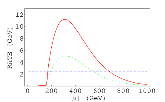
Figure 4: $\Gamma_{Y}$ (solid red line), $\bar{\Gamma}_{Y}$ (dashed green line), and $\Gamma_{Y}^{\rm scattering}$ (dashed straight blue line) in units of GeV as a function of $\mu$ (GeV), for $T=100$ GeV and SUSY mass parameters as described in the text. In large regions of parameter space we find $\Gamma_{Y}^{\rm decay}>\Gamma_{Y}^{\rm scattering}$.

IV Solving the Transport Equations and Phenomenology

The baryon asymmetry is seeded by the density of left-handed weak isodoublets $n_{L}=5Q+4T$ Cohen:1994ss ; HN , which we obtain by solving the transport equations (41). In this section we study the impact of $\Gamma_{Y}$ on the solution of the system (41) and on the overall baryon-to-entropy ratio $Y_{B}\equiv n_{B}/s$.

Before entering the details of our analysis, let us shortly recall the basic notation (see us and references therein) and describe the input MSSM parameters which will be used in the subsequent numerical explorations. The baryon-to-entropy ratio can be expressed as an integral of $n_{L}=5Q+4T$ in the unbroken phase:

$$Y_{B}=-\frac{n_{F}\Gamma_{\rm ws}}{2s}\,\frac{1}{D_{q}\lambda_{+}}\int_{-\infty}^{0}\ n_{L}(x)\,e^{-\lambda_{-}\,x}dx\ .$$ (44)

where $\Gamma_{\rm ws}$ is the weak sphaleron rate $\Gamma_{\rm ws}=6\kappa\alpha_{w}^{5}T$ (with $\kappa\simeq 20$ wsrate ), $n_{F}$ is the number of fermion families, $D_{q}$ is the quark diffusion constant, $v_{w}$ is the wall velocity and

$$\lambda_{\pm} = \frac{1}{2D_{q}}\,\left(v_{w}\pm\sqrt{v_{w}^{2}+4D_{q}{\cal R}}\right)$$

$${\cal R} = \Gamma_{\rm ws}\,\left[\frac{9}{4}\,\left(1+\frac{n_{\rm squark}}{6}\right)^{-1}+\frac{3}{2}\right]~{},$$ (45)

where $n_{\text{squark}}$ is the number of flavors of light squarks. Isolating the dependence on the CP-violating phases $\phi_{\mu}$ and $\phi_{A}$, $Y_{B}$ is conveniently parameterized as follows us :

$$Y_{B}=F_{1}\,\sin\phi_{\mu}\ +\ F_{2}\,\sin\left(\phi_{\mu}+\phi_{A}\right)\ ,$$ (46)

in terms of $F_{1}$ (arising from the Higgsino source) and $F_{2}$ (arising from the squark source).

In all the plots reported in this section, we adopt for the weak-scale SUSY parameters the reference values reported in Table 1, which are consistent with a strongly first-order electroweak phase transition and the constraints from precision electroweak physics as well as direct searches.

$\tan\beta=10$

$M_{\tilde{t}_{R}}=0$

$M_{\tilde{Q}}=1$ TeV

$M_{2}=A_{t}=200$ GeV

$m_{H_{u}}^{2}=-(100\,{\rm GeV})^{2}$

$m_{H_{d}}^{2}=0$

$m_{A}=150$ GeV

$100\ {\rm GeV}<|\mu|<400\ {\rm GeV}$

Table 1: Reference values of weak-scale SUSY parameters.

Note that a CP-odd Higgs mass $m_{A}=150$ GeV translates into $\Delta\beta\sim 0.015$ bubble . From the reference values of Table 1 one can derive typical values for the bubble wall velocity and thickness, for which we use $v_{w}=0.05$  John:2000zq and $L_{w}=25/T$  bubble . With this choice of parameters one has $F_{2}\sim 10^{-3}F_{1}$.

We now discuss in greater detail the role of Yukawa-induced rates on the transport equations.

IV.1 Revisiting the approximation of fast $\mathbf{\Gamma_{Y}}$: need for numerical solution

Starting with the work HN , the conventional practice has been to solve the system of transport equations (41) under the assumption that the rate $\Gamma_{Y}$ of Yukawa-induced processes  is “fast” compared to all other relevant time-scales, thereby ensuring a chemical equilibrium condition among $H$, $Q$, and $T$. Doing so allows one to obtain analytic expressions for $Y_{B}$. The assumption of fast Yukawa interactions is well justified in the unbroken phase ahead of the advancing bubble wall, where a particle may diffuse for a period characterized by the the inverse of the diffusion rate $\Gamma_{\rm diff}=v_{w}^{2}/D$ before the bubble wall catches it. In order for Yukawa processes to be effective in this region, they must act quickly on the time scale $\Gamma_{\rm diff}^{-1}$, and one, indeed, finds that $\Gamma_{Y}\gg\Gamma_{\rm diff}$ for typical values of the diffusion constants Joyce:1994fu ; Joyce:1994zn and wall velocity. In the broken electroweak phase, however, $\Gamma_{\rm diff}^{-1}$ is no longer the only relevant time scale. In addition, Yukawa processes must compete with scattering from the spacetime-varying Higgs vevs that leads to relaxation of chiral charge and Higgs supermultiplet densities. Importantly, the corresponding rates ($\Gamma_{M}$ and $\Gamma_{H}$, respectively) are as large as or larger than $\Gamma_{Y}$ – even after including the ${\cal O}(\alpha_{s}^{0})$ contributions to $\Gamma_{Y}$. As a result, the interplay of these competing processes within the bubble wall is significant, and imposing the condition of $\Gamma_{Y}$-induced chemical equilibrium is not justified.

To make this key point more explicit, we have solved the transport equations in powers of $1/\Gamma_{Y,ss}$ and analyzed the magnitude of the corrections to the $\Gamma_{Y,ss}\to\infty$ limit. Explicit details are given in Appendix C, where we point out that the most important correction was missed in previous analytic approaches to this problem – namely the correction to the $H$ density induced by an effective shift in the source $S_{\tilde{H}}^{CP\!\!\!\!\!\!\!\!\raisebox{0.0pt}{\small$\diagup$}}$. The analysis of Appendix C implies that fractional corrections to the baryon asymmetry to first order in $1/\Gamma_{Y}$ read

$$\frac{\delta Y_{B}}{Y_{B}}\sim\left(\frac{\Gamma_{H}}{\Gamma_{Y}}\right)\frac{\sqrt{r_{\Gamma}}\,\Gamma_{M}^{-}\,L_{w}}{\sqrt{\bar{D}(\Gamma_{M}^{-}+\Gamma_{H})}}$$ (47)

where $r_{\Gamma}\sim 0.07$ . Substituting the earlier estimates of $\Gamma_{H}$ and $\Gamma_{M}^{-}$ HN into this expression, we find $\delta Y_{B}/Y_{B}\sim 0.1$ – indeed a small correction. However, when using $\Gamma_{H}$, $\Gamma_{M}^{-}$ and $\Gamma_{Y}$ as calculated in Ref. us and the present work within the CTP framework, we find much larger corrections: $\delta Y_{B}/Y_{B}\sim\mathcal{O}(1)$. This difference is due primarily to the larger values of $\Gamma_{H}$ and $\Gamma_{M}$ obtained in our framework us (even off resonance) compared to previous calculations Joyce:1994fu ; Joyce:1994zn ; HN .

Figure 5: We plot here the ratio $F_{1}/Y_{B}^{\rm WMAP}$ versus $\Gamma_{Y}$ for two values of the SUSY $\mu$ parameter: $|\mu|=200$ GeV (solid line) and $|\mu|=250$ GeV (dashed line), corresponding to on-resonance and off-resonance baryogenesis, respectively. All other parameters are fixed at the reference values of Table 1. We use the central value $Y_{B}^{\rm WMAP}=9.2\times 10^{-11}$ wmap .

The above considerations imply that in order to avoid $\mathcal{O}(1)$ uncertainties in the calculation of $Y_{B}$, one requires a full numerical solution of the system (41). In order to quantify the effect, we plot in Fig. 5 the ratio $F_{1}/Y_{B}^{\rm WMAP}$ versus $\Gamma_{Y}$ for two values of the SUSY $\mu$ parameter: $|\mu|=200$ GeV (solid line) and $|\mu|=250$ GeV (dashed line), corresponding to on-resonance and off-resonance baryogenesis, respectively. All other parameters are fixed as in Table 1. Typical values of $\Gamma_{Y}$ lie in the range $5-10$ GeV (see Fig. 4). The curves in Fig. 5 illustrate two key points of the Yukawa-induced dynamics:

• Efficient chargino/neutralino-mediated baryogenesis occurs for $\Gamma_{Y}\gg v_{w}^{2}/D_{h}\sim 0.0025$ GeV, as the Higgs supermultiplet density $H$ injected in the unbroken phase is efficiently converted into LH top-quark density (fueling sphaleron processes) before the bubble catches up. Inclusion of the $\mathcal{O}(\alpha_{s}^{0})$ terms in $\Gamma_{Y}$ affects $Y_{B}$ at the $10-20\%$ level, as one is already in the plateau region in Fig. 5.

• As $\Gamma_{Y}$ increases (keeping all other rates fixed) the baryon asymmetry reaches a maximum and then starts decreasing towards its asymptotic value. This behavior can be understood qualitatively as follows. In the non-resonant case (dashed line), as $\Gamma_{Y}$ increases, Yukawa induced processes start to complete with $\Gamma_{H}$ inside the bubble wall, thereby transferring $H$ density to $Q,T$ densities. The latter subsequently relax away due to $\Gamma_{M}^{-}$ processes or diffuse very inefficiently into the unbroken phase. This effect is less pronounced in the resonant case (solid line), where $Y_{B}$ first grows as $\Gamma_{Y}$ becomes more efficient compared to diffusion ahead of the bubble wall, but then saturates due to the presence of resonantly-enhanced Higgs supermultiplet relaxation within the plasma.

Summarizing, the main message emerging from Fig. 5 is the following: keeping $\Gamma_{Y}$ finite and in the realistic range (few GeV) can increase $Y_{B}$ by a factor between $20\%$ (resonant case) and $100\%$ (nonresonant case) compared to the $\Gamma_{Y}\to\infty$ limit.

IV.2 Phenomenology update

Figure 6: $F_{1}$ (solid line) and $F_{2}$ (dashed line) versus $|\mu|$ with all other parameters fixed at the reference values of Table 1.

In a consistent analysis $\Gamma_{Y}$ should not be treated as an independent quantity (as we did in the last section for illustrative purposes) but rather as a function of the MSSM parameters (as we did in Section III). Doing so after numerically solving the transport equations, we study the behavior of $F_{1,2}$ (Eq. (46)) as a function of the MSSM parameters. For illustration, we show in Fig. 6 the dependence of $F_{1}$ (solid line) and $F_{2}$ (dashed line) on $|\mu|$, with all other input as in Table 1. The plot highlights the resonant behavior of $F_{1}$ discussed in Carena:1997gx ; riotto ; us . The behavior of $F_{2}$ follows from the fact that $F_{2}$ is proportional to $|\mu|(\Gamma_{H}+\Gamma_{M}^{-})^{-1/2}$: the dip at $|\mu|\sim M_{2}\sim 200$ GeV reflects the resonant enhancement of $\Gamma_{H}$. The overall scale of $F_{1,2}$ is set by $\Delta\beta$ which in turn depends crucially on the CP-odd Higgs mass $m_{A}$ bubble : here we use $m_{A}=150$ GeV but one should keep in mind that higher values of $m_{A}$ can lead to sizable suppression of $F_{1,2}$.

Finally, we investigate the impact of electric dipole moment (EDM) searches on this particular EWB scenario. It has long been recognized that, given the spectrum of supersymmetric particles, constraints from the electron Regan:2002ta , neutron neutron , and nuclear Romalis:2000mg EDMs pose tight limits on the size of CP-violating phases (for a review see Pospelov:2005pr ). These could ultimately enter in conflict with the requirement of successful baryon asymmetry generation, making EDM searches a great discriminating tool among theories of baryogenesis.

Figure 7: Allowed bands in the $\phi_{\mu}$–$\phi_{A}$ plane implied by consistency with the $95\%$ C.L. limits on electron and neutron EDMs and baryogenesis. The solid lines correspond to the constraint from the electron EDM ($|d_{e}|<1.9\times 10^{-27}e\cdot{\rm cm}$ Regan:2002ta ), and the dashed lines correspond to the neutron EDM ($|d_{n}|<3.6\times 10^{-26}e\cdot{\rm cm}$ neutron ). These EDM constraints correspond to sfermion masses ($m_{\tilde{f}}$) fixed at 1 TeV. The shaded EWB band is the region consistent with $Y_{B}$ from BBN PDG at 95$\%$ C.L. (which includes the $Y_{B}$ range from WMAP wmap ). In the left-hand panel we use $|\mu|=M_{2}=200$ GeV (resonance peak), while in the right-hand panel we use $M_{2}=200$ GeV and $|\mu|=250$ GeV (off resonance). The other supersymmetric masses are as specified in the text.

To illustrate this point we plot in Fig. 7 the allowed bands in the $\phi_{\mu}$–$\phi_{A}$ plane resulting from present limits on electron and neutron EDMs and successful baryogenesis, for a given choice of the SUSY mass parameters. Here, we have employed one-loop SUSY contributions Ibrahim:1997gj . We take the first- and second-generation sfermions, as well as the gluinos, all degenerate at 1 TeV, while all other input is fixed as in Table 1. In the left-hand panel we use $M_{2}=|\mu|=200$ GeV (resonance peak), while in the right we use $M_{2}=200$ GeV, $|\mu|=250$ GeV.

Figure 7 illustrates the complementarity of various EDM measurements in constraining the new CP-violating phases in general. It also shows that in this particular scenario it is the electron EDM that poses the strongest constraints on electroweak baryogenesis. In order to quantify the dependence of the EDM constraints on the heavy sfermion masses, we plot in Fig. 8 the region in the $|\phi_{\mu}|$-$|\mu|$ plane that is consistent with EWB (gray shaded band) along with the $|d_{e}^{\text{1-loop}}|=1.9\times 10^{-27}\,{\rm e}\cdot\,{\rm cm}$ (95 $\%$ C.L. limit) curves for various values of the first generation slepton masses (assumed degenerate). For a given slepton mass, the region in the $|\phi_{\mu}|$-$|\mu|$ plane consistent with EDM constraints lies below the dashed line. In the same figure, we also plot the $\left\lvert d_{e}^{\text{2-loop}}\right\rvert=1.9\times 10^{-27}\,\text{e}\cdot\text{cm}$ curve (solid red line) from two-loop SUSY contributions 2-loop .

Figure 8: We plot in the $|\phi_{\mu}|$-$|\mu|$ plane the region consistent with EWB (gray shaded band), the $|d_{e}^{\text{1-loop}}|=1.9\times 10^{-27}\,{\rm e}\cdot\,{\rm cm}$ (95 $\%$ C.L. limit) curves for various values of the first-generation slepton masses (dashed horizontal lines), and the $|d_{e}^{\text{2-loop}}|=1.9\times 10^{-27}\,{\rm e}\cdot\,{\rm cm}$ curve. For a given choice of mass parameters, the allowed parameter region lies below the EDM curves. The baryon-to-entropy ratio is required to be in the range $4.8\times 10^{-11}<Y_{B}<9.8\times 10^{-11}$ PDG , and the SUSY parameters are as in Table 1.

Several key features emerge from Figs. 7 and 8:

• In the range of $\mu$ and $M_{2}$ we are considering, $\left\lvert d_{e}\right\rvert$ is dominated by the one-loop contributions for slepton masses below 1–2 TeV, while the two-loop effects become dominant for slepton masses larger than 2–3 TeV.

• In the case of resonant EWB, which requires the smallest amount of CP violation, the electron EDM constraint requires slepton masses to be heavier than 1 TeV.

• Two-loop contributions to $d_{e}$ imply that EWB cannot occur too far off resonance (see Fig. 8), even in the limit of very heavy sleptons.

Additional constraints on higgsino-mediated electroweak baryogenesis do arise from the phenomenology of indirect dark matter detection in the MSSM, and they are investigated in Ref. profumoetal .

Before concluding, we emphasize that the constraints implied by Figs. 7 and 8 are specific to the MSSM, and that the extensions of the MSSM discussed in Ref. nonminimal and elsewhere can lead to different phenomenological conclusions. In particular, extended Higgs sector models with additional scalar degrees of freedom can give rise to a strong, first-order electroweak phase transition without requiring a light ${\tilde{t}}_{R}$. In this case, resonances in the stop sector may enhance the importance of CP-violation associated with the tri-scalar terms (e.g., $\phi_{A}$), and the information provided by the neutron and neutral atom EDM searches would become more important than for the MSSM scenario considered here. In addition, we also note that there could exist additional, $\mathcal{O}(1)$ corrections to $Y_{B}$ associated with computations of the sphaleron rates, bubble profile, and Majorana gaugino transport that we have not addressed here.

V Conclusions

The present work is part of a broader program initiated in us whose goal is to systematically reduce uncertainties in EWB calculations induced by transport phenomena. The main new results of this work are:

• We have calculated the contribution to the quantum Boltzmann equations due to decays and inverse decays induced by tri-scalar and Yukawa-type interactions. We have performed the calculation in the Closed Time Path formalism to leading non-trivial order in the ratios $\varepsilon_{\mu}=\mu/T$, $\varepsilon_{p}=\Gamma/\omega$, $\varepsilon_{d}=v_{w}k_{\rm eff}/\omega$.

• Specializing to the case of MSSM, we have derived the (inverse) decay rate due to top-quark Yukawa interactions, their supersymmetric tri-scalar counterparts, and the soft SUSY-breaking tri-scalar interactions proportional to $y_{t}$. These rates are of ${\cal O}(\alpha_{s}^{0})$, and – when not vanishing due to threshold effects – they can be of comparable size or larger than the ${\cal O}(\alpha_{s})$ contributions from scattering processes.

• We have revisited the fast-$\Gamma_{Y}$ approximation HN , which consists in taking the rate $\Gamma_{Y}$ of Yukawa-induced processes as large compared to all other relevant time-scales. We have found previously-unnoticed corrections to the baryon density that enter at linear order in the $1/\Gamma_{Y}$-expansion, whose inclusion shows that this expansion in fact breaks down. The approximation is sound in the unbroken phase, where Yukawa processes are, indeed, fast on the scale of diffusion processes. But in the broken phase, the rates $\Gamma_{M}$, $\Gamma_{H}$ associated with relaxation processes can be as large as or larger than $\Gamma_{Y}$, even after including the ${\cal O}(\alpha_{s}^{0})$ contributions to $\Gamma_{Y}$. The interplay of these competing processes is quite significant, and a quantitative analysis requires performing a numerical solution to the transport equations for realistic, finite values of $\Gamma_{Y}$. For the parameter choices we considered, keeping $\Gamma_{Y}$ finite can increase $Y_{B}$ by a factor between $20\%$ and $100\%$ compared to the $\Gamma_{Y}\to\infty$ limit.

• We have updated our previous us analysis of the connection between EDM constraints and EWB. Even within present uncertainties, the simultaneous requirement of successful EWB and consistency with EDM upper limits, poses stringent constraints on the size of SUSY CP violating phases and mass spectrum. For example, for any value of the CP violating phases, successful baryogenesis and one-loop EDM constraints force the slepton masses to be heavier than $\sim 1$ TeV. Bounds of this type will be sharpened by future EDM experiments and can be tested at future collider experiments.

Appendix A $\mathcal{I}_{B}$ and $\mathcal{I}_{F}$ in terms of one-dimensional integrals

Performing the $\omega_{L}$ integral in Eq. (18) and the $\omega_{\phi}$ integral in Eq. (22) yields

$$\begin{split}&\mathcal{I}_{B}(A_{s}\,;\,m_{R},m_{L},m_{H})=\frac{\left\lvert A_{s}\right\rvert^{2}}{16\pi^{3}}\,\int_{m_{R}}^{\infty}d\omega_{R}\,h_{B}(\omega_{R})\\ &\ \ \ \times\biggl{\{}\log\left(\frac{e^{\omega_{R}/T}-e^{\omega_{L}^{+}/T}}{e^{\omega_{R}/T}-e^{\omega_{L}^{-}/T}}\frac{e^{\omega_{L}^{-}/T}-1}{e^{\omega_{L}^{+}/T}-1}\right)\bigl{[}\theta(m_{R}-m_{L}-m_{H})-\theta(m_{L}-m_{R}-m_{H})\bigr{]}\\ &\qquad\qquad\qquad\qquad\quad+\log\left(\frac{e^{-\omega_{R}/T}-e^{\omega_{L}^{+}/T}}{e^{-\omega_{R}/T}-e^{\omega_{L}^{-}/T}}\frac{e^{\omega_{L}^{-}/T}-1}{e^{\omega_{L}^{+}/T}-1}\right)\theta(m_{H}-m_{R}-m_{L})\biggr{\}}\end{split}$$ (48)

and

$$\begin{split}&\mathcal{I}_{F}(m_{1},m_{2},m_{\phi})=-\frac{1}{16\pi^{3}}\,\left(m_{1}^{2}+m_{2}^{2}-m_{\phi}^{2}\right)\,\int_{m_{1}}^{\infty}d\omega_{1}h_{F}(\omega_{1})\\ &\ \ \ \times\biggl{\{}\log\left(\frac{e^{\omega_{\phi}^{+}/T}-1}{e^{\omega_{\phi}^{-}/T}-1}\frac{e^{\omega_{\phi}^{-}/T}+e^{\omega_{1}/T}}{e^{\omega_{\phi}^{+}/T}+e^{\omega_{1}/T}}\right)[\theta(m_{1}-m_{2}-m_{\phi})-\theta(m_{\phi}-m_{1}-m_{2})\bigr{]}\\ &\qquad\qquad\qquad\quad+\log\left(\frac{e^{\omega_{\phi}^{+}/T}-1}{e^{\omega_{\phi}^{-}/T}-1}\frac{e^{\omega_{\phi}^{-}/T}+e^{-\omega_{1}/T}}{e^{\omega_{\phi}^{+}/T}+e^{-\omega_{1}/T}}\right)\theta(m_{2}-m_{1}-m_{\phi})\biggr{\}}\end{split}$$ (49)

where

$$h_{F,B}(x)=-\frac{e^{x/T}}{(e^{x/T}\pm 1)^{2}}\ .$$ (50)

Appendix B Details of the source derivation

In this Appendix we give some details of the derivation of the source terms reported in Section III. We first relate the scalar Higgs chemical potentials $\mu_{H_{u,d}}$ to the Higgsino chemical potential $\mu_{\tilde{H}}$ and then show how to further simplify the final expression by use of mass relations among weak doublet partners.

Recall that the Higgsino chemical potential $\mu_{\tilde{H}}$ corresponds to the vector charges, $n_{\tilde{H}^{+,0}}=\bar{\Psi}_{\tilde{H}^{+,0}}\gamma^{0}\Psi_{\tilde{H}^{+,0}}$, for the Dirac fields introduced in Eq. (29), which combine $u$- and $d$-type Higgsino densities. To determine the scalar Higgs density that is kept in equilibrium with the Higgsino vector charge density via gaugino interactions, we examine their interactions in the MSSM Lagrangian, written in terms of the Dirac fields $\Psi_{\tilde{H}^{+,0}}$, and the four-component gaugino fields:

$$\Psi_{\tilde{W}^{+}}=\begin{pmatrix}\tilde{W}^{+}\\ \tilde{W}^{-{\dagger}}\end{pmatrix},\qquad\Psi_{\tilde{W}^{0}}=\begin{pmatrix}\tilde{W}_{3}\\ \tilde{W}_{3}^{\dagger}\end{pmatrix},\qquad\Psi_{\tilde{B}}=\begin{pmatrix}\tilde{B}\\ \tilde{B}^{\dagger}\end{pmatrix}.$$ (51)

The charged wino field $\Psi_{\tilde{W}^{+}}$ is a Dirac spinor, for which a vector charge density can also be defined, while the neutral fields $\Psi_{\tilde{W}^{0},\tilde{B}}$ are Majorana spinors, whose vector charge density is zero. In terms of these fields, the Higgs-Higgsino-gaugino interactions are:

$$\begin{split}\mathcal{L}_{H\tilde{H}\tilde{V}}=&-\frac{g_{1}}{\sqrt{2}}\Bigl{[}\bar{\Psi}_{\tilde{H}^{+}}(H_{d}^{-*}P_{L}+e^{i\phi_{\mu}}H_{u}^{+}P_{R})\Psi_{\tilde{B}}+\bar{\Psi}_{\tilde{H}^{0}}(H_{d}^{0*}P_{L}-e^{i\phi_{\mu}}H_{u}^{0}P_{R})\Psi_{\tilde{B}}\Bigr{]}\\ &-\frac{g_{2}}{\sqrt{2}}\Bigl{[}\bar{\Psi}_{\tilde{H}^{+}}(-H_{d}^{-*}P_{L}+e^{i\phi_{\mu}}H_{u}^{+}P_{R})\Psi_{\tilde{W}^{0}}+\bar{\Psi}_{\tilde{H}^{0}}(H_{d}^{0*}P_{L}+e^{i\phi_{\mu}}H_{u}^{0}P_{R})\Psi_{\tilde{W}^{0}}\Bigr{]}\\ &-g_{2}\Bigl{[}\bar{\Psi}_{\tilde{H}^{+}}(H_{d}^{0*}P_{L}+e^{i\phi_{\mu}}H_{u}^{0}P_{R})\Psi_{\tilde{W}^{+}}+\bar{\Psi}_{\tilde{W}^{+}}(H_{d}^{-*}P_{L}-e^{i\phi_{\mu}}H_{u}^{+}P_{R})\Psi_{\tilde{H}^{0}}^{C}\Bigr{]}\\ &+\text{h.c.}\end{split}$$ (52)

The combinations of scalar fields appearing in each term of Eq. (52) tell us which densities are kept in equilibrium with the Higgsino densities by fast gaugino interactions. To illustrate, consider the second term on the RHS that couples the ${\tilde{H}}_{0}$ and ${\tilde{B}}_{0}$ fields to the neutral Higgs fields. Using $\mu_{\tilde{B}}=0$ we see from Eqs. (20,21) that this term in $\mathcal{L}_{H\tilde{H}\tilde{V}}$ will generate source terms for ${\tilde{H}}_{0}$ given by

$$S_{\tilde{H}^{0}} = -\frac{g_{1}^{2}}{2}\left[(\mu_{{\tilde{H}}^{0}}-\mu_{H_{u}^{0}})\mathcal{I}_{F}(m_{\tilde{H}^{0}},m_{\tilde{B}},m_{H_{u}^{0}})+(\mu_{{\tilde{H}}^{0}}+\mu_{H_{d}^{0}})\mathcal{I}_{F}(m_{\tilde{H}^{0}},m_{\tilde{B}},m_{H_{d}^{0}})\right]$$ (53)

$$= \quad\frac{g_{1}^{2}}{2}\left[(\mu_{H^{0}}-\mu_{{\tilde{H}}^{0}})\mathcal{I}_{F,\,H}^{(+)}+\mu_{h^{0}}\mathcal{I}_{F,\,H}^{(-)}\right]\ \ \ ,$$ (54)

where

$$\mu_{H^{0}} \equiv =\frac{1}{2}\left(\mu_{H_{u}^{0}}-\mu_{H_{d}^{0}}\right)$$ (55)

$$\mu_{h^{0}} \equiv =\frac{1}{2}\left(\mu_{H_{u}^{0}}+\mu_{H_{d}^{0}}\right)$$ (56)

$$\mathcal{I}_{F,\,H}^{(\pm)} = \mathcal{I}_{F}(m_{\tilde{H}^{0}},m_{\tilde{B}},m_{H_{u}^{0}})\pm\mathcal{I}_{F}(m_{\tilde{H}^{0}},m_{\tilde{B}},m_{H_{d}^{0}})\ \ \ .$$ (57)

Similar expressions follow from the other terms in Eq. (52) (assuming the ${\tilde{W}}$ densities vanish). The assumption of “fast” supergauge interactions then leads to:

$$\mu_{H} \equiv \frac{1}{2}\left(\mu_{H_{u}}-\mu_{H_{d}}\right)=\mu_{\tilde{H}}$$ (58)

$$\mu_{h} \equiv \frac{1}{2}\left(\mu_{H_{u}}+\mu_{H_{d}}\right)$$ (59)

and

$$\mu_{H_{u}}=\mu_{H}+\mu_{h}\qquad\mu_{H_{d}}=\mu_{h}-\mu_{H}\ \ \ ,$$ (60)

where $\mu_{H}$ and $\mu_{h}$ refer to the common chemical potentials for the charged and neutral Higgs scalars. Adding together the top and stop sources in Eq. (32,33) and using the relations (34,58,60) gives for the Yukawa source for the density $T$:

$$\begin{split}S_{T}^{Y}=-N_{C}y_{t}^{2}\biggl{\{}(\mu_{T}-\mu_{Q}-\mu_{H})\Bigl{[}&\mathcal{I}_{B}(A_{t};m_{\tilde{t}_{R}},m_{\tilde{t}_{L}},m_{H_{u}^{0}})+\mathcal{I}_{B}(A_{t};m_{\tilde{t}_{R}},m_{\tilde{b}_{L}},m_{H_{u}^{+}})\\ +&\mathcal{I}_{B}(\mu;m_{\tilde{t}_{R}},m_{\tilde{t}_{L}},m_{H_{d}^{0}})+\mathcal{I}_{B}(\mu;m_{\tilde{t}_{R}},m_{\tilde{b}_{L}},m_{H_{d}^{-}})\\ +&\mathcal{I}_{F}(m_{\tilde{H}^{+}},m_{t_{L}},m_{\tilde{t}_{R}})+\mathcal{I}_{F}(m_{\tilde{H}^{0}},m_{b_{L}},m_{\tilde{t}_{R}})\\ +&\mathcal{I}_{F}(m_{t_{R}},m_{t_{L}},m_{H_{u}^{0}})+\mathcal{I}_{F}(m_{t_{R}},m_{b_{L}},m_{H_{u}^{+}})\\ +&\mathcal{I}_{F}(m_{t_{R}},m_{\tilde{H}^{0}},m_{\tilde{t}_{L}})+\mathcal{I}_{F}(m_{t_{R}},m_{\tilde{H}^{+}},m_{\tilde{b}_{L}})\Bigr{]}\\ +\mu_{h}\Bigl{[}&\mathcal{I}_{B}(\mu;m_{\tilde{t}_{R}},m_{\tilde{t}_{L}},m_{H_{d}^{0}})+\mathcal{I}_{B}(\mu;m_{\tilde{t}_{R}},m_{\tilde{t}_{L}},m_{H_{d}^{-}})\\ -&\mathcal{I}_{B}(A_{t};m_{\tilde{t}_{R}},m_{\tilde{t}_{L}},m_{H_{u}^{0}})-\mathcal{I}_{B}(A_{t};m_{\tilde{t}_{R}},m_{\tilde{b}_{L}},m_{H_{u}^{+}})\\ -&\mathcal{I}_{F}(m_{t_{R}},m_{t_{L}},m_{H_{u}^{0}})-\mathcal{I}_{F}(m_{t_{R}},m_{b_{L}},m_{H_{u}^{+}})\Bigr{]}\biggr{\}}\end{split}$$ (61)

We can simplify further by noting that the masses of weak doublet partners are the same:

$$m_{t_{L}} =m_{b_{L}}\equiv m_{Q}$$ (62a)

$$m_{\tilde{t}_{L}} =m_{\tilde{b}_{L}}\equiv m_{\tilde{Q}}$$ (62b)

$$m_{H_{u}^{+}} =m_{H_{u}^{0}}\equiv m_{H_{u}}$$ (62c)

$$m_{H_{d}^{-}} =m_{H_{d}^{0}}\equiv m_{H_{d}}$$ (62d)

$$m_{\tilde{H}^{+}} =m_{\tilde{H}^{0}}=\left\lvert\mu\right\rvert~{}.$$ (62e)

With the notation for the masses introduced here we arrive at our final result of Eq. (40).

Appendix C Analytic corrections of $\mathcal{O}(1/\Gamma_{Y,ss})$

In this Appendix we solve the transport equations in powers of $1/\Gamma_{Y,ss}$ and show that the analytic solutions obtained in the $\Gamma_{Y}\to\infty$ limit can receive $\mathcal{O}(1)$ corrections for realistic choices of all the competing rates ($\Gamma_{Y,H,M}$).

The zeroth-order solution in $1/\Gamma_{Y,ss}$ is obtained by considering the combination of Eqs. (41) that is independent of $\Gamma_{Y}$ and $\Gamma_{ss}$. Letting $D_{h}$ and $D_{q}$ be the diffusion constants for Higgs and quark superfields, respectively [see Eq. (13)], letting the densities be a function of ${\bar{z}}=\left\lvert\mathbf{x}+\mathbf{v}_{w}t\right\rvert$ (the co-moving distance from the bubble surface along its normal), and neglecting small corrections proportional to $\Gamma_{M}^{+}$ for simplicity, we obtain:

$$\begin{split}D_{q}[2T^{\prime\prime}(\bar{z})+Q^{\prime\prime}(\bar{z})]+D_{h}H^{\prime\prime}(\bar{z})&-v_{w}[2T^{\prime}(\bar{z})+Q^{\prime}(\bar{z})+H^{\prime}(\bar{z})]\\ =&\Gamma_{M}^{-}(\bar{z})\biggl{[}\frac{T(\bar{z})}{k_{T}}-\frac{Q(\bar{z})}{k_{Q}}\biggr{]}+\Gamma_{h}(\bar{z})\frac{H(\bar{z})}{k_{H}}-S_{TOT}^{CP\!\!\!\!\!\!\!\!\raisebox{0.0pt}{\small$\diagup$}}(\bar{z})\end{split}$$ (63)

where $S_{TOT}^{CP\!\!\!\!\!\!\!\!\raisebox{0.0pt}{\small$\diagup$}}=S_{\tilde{H}}^{CP\!\!\!\!\!\!\!\!\raisebox{0.0pt}{\small$\diagup$}}+S_{\tilde{t}}^{CP\!\!\!\!\!\!\!\!\raisebox{0.0pt}{\small$\diagup$}}$ and $f^{\prime}=\partial f/\partial{\bar{z}}$. The approximate chemical equilibrium enforced by Yukawa and strong sphaleron processes implies that the combinations

$$\delta_{Y} = \frac{T}{k_{T}}-\frac{Q}{k_{Q}}-\frac{H}{k_{H}}$$ (64)

$$\delta_{ss} = -\left(\frac{2Q}{k_{Q}}-\frac{T}{k_{T}}+\frac{9(Q+T)}{k_{B}}\right)$$

tend to zero in the limit $\Gamma_{Y,ss}\to\infty$, so that we can formally expand in $1/\Gamma_{Y,ss}$ and treat for bookkeeping purposes $\delta_{Y}\sim 1/\Gamma_{Y}$ and $\delta_{ss}\sim 1/\Gamma_{ss}$. The relations between the $Q$, $T$, and $H$ densities, up to order $1/\Gamma_{Y,ss}$ are then:

$$Q = \frac{k_{Q}(k_{B}-9k_{T})}{k_{H}(9k_{T}+9k_{Q}+k_{B})}\,\left(H+k_{H}\delta_{Y}\right)-\frac{k_{B}k_{Q}}{(9k_{T}+9k_{Q}+k_{B})}\,\delta_{ss}$$ (65)

$$T = \frac{k_{T}(2k_{B}+9k_{Q})}{k_{H}(9k_{T}+9k_{Q}+k_{B})}\,\left(H+k_{H}\delta_{Y}\right)-\frac{k_{B}k_{T}}{(9k_{T}+9k_{Q}+k_{B})}\,\delta_{ss}~{}.$$

Substituting these expressions back into Eq. (63), we obtain the equation for $H$:

$$v_{w}H^{\prime}(\bar{z})-{\bar{D}}H^{\prime\prime}(\bar{z})=-{\bar{\Gamma}}H(\bar{z})+{\bar{S}}(\bar{z})+\delta{\bar{S}}(\bar{z})$$ (66)

where

$${\bar{D}} = \frac{D_{h}\Delta+D_{q}K}{(K+\Delta)}$$

$${\bar{\Gamma}} = \frac{\Delta}{k_{H}(K+\Delta)}\left(\Gamma_{M}^{-}+\Gamma_{H}\right)$$

$${\bar{S}} = \frac{\Delta}{(K+\Delta)}S_{TOT}^{CP\!\!\!\!\!\!\!\!\raisebox{0.0pt}{\small$\diagup$}}$$ (67)

$$K = 9k_{T}k_{Q}+k_{B}k_{Q}+4k_{T}k_{B}$$

$$\Delta = k_{H}\left(9k_{T}+9k_{Q}+k_{B}\right)\ \ \ ,$$

and

$$\delta{\bar{S}}=\frac{k_{H}}{(K+\Delta)}\biggl{[}k_{B}(2k_{T}+k_{Q})(v_{w}\delta_{ss}^{\prime}-D_{q}\delta_{ss}^{\prime\prime})-K(v_{w}\delta_{Y}^{\prime}-D_{q}\delta_{Y}^{\prime\prime})-(\Delta/k_{H})\Gamma_{M}^{-}\delta_{Y}\biggr{]}$$ (68)

represents a correction to the effective source $\bar{S}$ for the Higgs density $H$. The functions $\delta_{Y}$ and $\delta_{ss}$ appearing in Eq. (68) are determined by substituting the lowest order solution $H_{0}$ into Eqs. (41) and read:

$$\delta_{Y}(\bar{z}) =-\frac{1}{\Gamma_{Y}}\biggl{[}D_{h}H_{0}^{\prime\prime}(\bar{z})-v_{w}H_{0}^{\prime}(\bar{z})-\Gamma_{H}(\bar{z})\frac{H_{0}(\bar{z})}{k_{H}}+S_{\tilde{h}}(\bar{z})\biggr{]}$$ (69a)

$$\delta_{ss}(\bar{z}) =-\frac{1}{\Gamma_{ss}}\frac{k_{B}}{k_{H}}\frac{k_{Q}+2k_{T}}{k_{B}+9k_{T}+9k_{Q}}\bigl{[}D_{q}H_{0}^{\prime\prime}(\bar{z})-v_{w}H_{0}^{\prime}(\bar{z})\bigr{]}.$$ (69b)

Although in the unbroken phase $\delta_{Y,ss}\sim\Gamma_{\rm diff}/\Gamma_{Y,ss}\times H_{0}\ll H_{0}$, in the broken phase, they can be sizable, with $\delta_{Y}\gg\delta_{ss}$.

All previous treatments have neglected the $\delta\bar{S}$ term in Eq. (66) and thus find only the leading-order solution for $H$. Then the only $1/\Gamma_{Y,ss}$ effects appear to be the $\delta_{Y,ss}$ terms in Eqs. (65). However, $\delta\bar{S}$ induces $\mathcal{O}(1/\Gamma_{Y,ss})$ corrections to the density $H$ obtained by solving Eq. (66), which must be substituted back into Eqs. (65) to give the full $Q,T$ densities to order $1/\Gamma_{Y,ss}$. Using the simplified bubble wall profile as in Ref. us (with constant sources in the region $0<{\bar{z}}<L_{w}$), the explicit solution to Eq. (66) in the region of unbroken electroweak symmetry (${\bar{z}}<0$), that drives the weak sphaleron processes, reads

$$H_{<}({\bar{z}})=\left[\frac{1}{{\bar{D}}\kappa_{+}}\,\int_{0}^{\infty}dy\,e^{\rm-\kappa_{+}y}\,\left({\bar{S}}(y)+\delta{\bar{S}}(y)\right)+\frac{\delta{\bar{S}}_{<}(0)}{v_{w}}\left(\frac{1}{\kappa_{+}}-{\bar{z}}\right)\right]e^{v_{w}{\bar{z}}/{\bar{D}}}\ \ \ ,$$ (70)

with

$$\kappa_{\pm}=\frac{1}{2}\left(v_{w}\pm\sqrt{v_{w}^{2}+4{\bar{\Gamma}}{\bar{D}}}\right)\ ,$$ (71)

and $\delta\bar{S}_{<}(0)$ is the value that $\delta\bar{S}$ takes at $\bar{z}=0$ approaching from the left. The ${\cal O}(1/\Gamma_{Y,ss})$ contributions to $H$ live in the terms containing $\delta{\bar{S}}$. The largest effect arises from the presence of $\delta{\bar{S}}(y)$ inside the integral. The overall size of $\delta\bar{S}$ is dominated by the term in Eq. (68) proportional to $\delta_{Y}\Gamma_{M}^{-}$. Moreover, the typical size of $\delta_{Y}$ is set by $(\Gamma_{H}/\Gamma_{Y})\cdot(H_{0}/k_{H})$, leading to:

$$\frac{\delta{\bar{S}}}{{\bar{S}}}\sim\left(\frac{\Gamma_{H}}{\Gamma_{Y}}\right)\frac{\sqrt{r_{\Gamma}}\,\Gamma_{M}^{-}\,L_{w}}{\sqrt{\bar{D}(\Gamma_{M}^{-}+\Gamma_{H})}}$$ (72)

with $r_{\Gamma}=\Delta/[k_{H}(K+\Delta)]\sim 0.07$ . Using earlier estimates of $\Gamma_{H}$ and $\Gamma_{M}^{-}$ HN , we find $\delta\bar{S}/\bar{S}\sim 0.1$, indeed a small correction. However, when using $\Gamma_{H}$, $\Gamma_{M}^{-}$ and $\Gamma_{Y}$ as calculated in Ref. us and the present work within the CTP framework, we find $\delta{\bar{S}}/{\bar{S}}\sim 1$, thus invalidating the assumption of fast $\Gamma_{Y}$ rates.

In conclusion, the large $\delta_{Y,ss}$ corrections in the broken phase induce large corrections to the effective source for the Higgs density, which in turn induce large corrections to $Q,T$ themselves. What past treatments have derived correctly are the $1/\Gamma_{Y,ss}$ corrections to the relation between $Q,T$, and $H$ (that is, Eq. (65)), but not the corrections to $H$ itself. Yet this correction, it turns out, is the biggest piece of all.

References

• (1) J. Erler and M. J. Ramsey-Musolf, Prog. Part. Nucl. Phys.  54, 351 (2005) [arXiv:hep-ph/0404291].
• (2) M. Pospelov and A. Ritz, Annals Phys.  318, 119 (2005) [arXiv:hep-ph/0504231].
• (3) A. G. Cohen, D. B. Kaplan and A. E. Nelson, Phys. Lett. B 336, 41 (1994) [arXiv:hep-ph/9406345].
• (4) P. Huet and A. E. Nelson, Phys. Rev. D 53, 4578 (1996) [arXiv:hep-ph/9506477].
• (5) M. Joyce, T. Prokopec and N. Turok, Phys. Rev. Lett.  75, 1695 (1995) [Erratum-ibid.  75, 3375 (1995)] [arXiv:hep-ph/9408339].
• (6) M. Joyce, T. Prokopec and N. Turok, Phys. Rev. D 53, 2930 (1996) [arXiv:hep-ph/9410281].
• (7) M. Trodden, Rev. Mod. Phys.  71, 1463 (1999) [arXiv:hep-ph/9803479].
• (8) A. Riotto, Phys. Rev. D 53, 5834 (1996) [arXiv:hep-ph/9510271].
• (9) A. Riotto, Phys. Rev. D 58, 095009 (1998) [arXiv:hep-ph/9803357].
• (10) M. Carena, J. M. Moreno, M. Quiros, M. Seco and C. E. M. Wagner, Nucl. Phys. B 599, 158 (2001) [arXiv:hep-ph/0011055].
• (11) M. Carena, M. Quiros, M. Seco and C. E. M. Wagner, Nucl. Phys. B 650, 24 (2003) [arXiv:hep-ph/0208043].
• (12) T. Konstandin, T. Prokopec and M. G. Schmidt, Nucl. Phys. B 716, 373 (2005) [arXiv:hep-ph/0410135].
• (13) T. Konstandin, T. Prokopec and M. G. Schmidt, Nucl. Phys. B 679, 246 (2004) [arXiv:hep-ph/0309291].
• (14) T. Konstandin, T. Prokopec, M. G. Schmidt and M. Seco, Nucl. Phys. B 738, 1 (2006) [arXiv:hep-ph/0505103].
• (15) C. Lee, V. Cirigliano and M. J. Ramsey-Musolf, Phys. Rev. D 71, 075010 (2005) [arXiv:hep-ph/0412354].
• (16) M. Carena, M. Quiros, A. Riotto, I. Vilja and C. E. M. Wagner, Nucl. Phys. B 503, 387 (1997) [arXiv:hep-ph/9702409].
• (17) C. Balazs, M. Carena, A. Menon, D. E. Morrissey and C. E. M. Wagner, Phys. Rev. D 71, 075002 (2005) [arXiv:hep-ph/0412264].
• (18) M. Laine and K. Rummukainen, Nucl. Phys. B 535, 423 (1998) [arXiv:hep-lat/9804019]; M. Laine and K. Rummukainen, Nucl. Phys. B 597, 23 (2001) [arXiv:hep-lat/0009025]; M. Laine, arXiv:hep-ph/0010275.
• (19) M. Pietroni, Nucl. Phys. B 402 (1993) 27 [arXiv:hep-ph/9207227], A. T. Davies, C. D. Froggatt and R. G. Moorhouse, Phys. Lett. B 372 (1996) 88 [arXiv:hep-ph/9603388], S. J. Huber and M. G. Schmidt, Nucl. Phys. B 606 (2001) 183 [arXiv:hep-ph/0003122], M. Bastero-Gil, C. Hugonie, S. F. King, D. P. Roy and S. Vempati, Phys. Lett. B 489, 359 (2000) [arXiv:hep-ph/0006198], J. Kang, P. Langacker, T. j. Li and T. Liu, Phys. Rev. Lett.  94, 061801 (2005) [arXiv:hep-ph/0402086], A. Menon, D. E. Morrissey and C. E. M. Wagner, Phys. Rev. D 70, 035005 (2004) [arXiv:hep-ph/0404184], C. Grojean, G. Servant and J. D. Wells, Phys. Rev. D 71, 036001 (2005) [arXiv:hep-ph/0407019], M. Carena, A. Megevand, M. Quiros and C. E. M. Wagner, Nucl. Phys. B 716, 319 (2005) [arXiv:hep-ph/0410352].
• (20) J. M. Cline and K. Kainulainen, Phys. Rev. Lett.  85, 5519 (2000) [arXiv:hep-ph/0002272].
• (21) J. M. Cline, M. Joyce and K. Kainulainen, JHEP 0007, 018 (2000) [arXiv:hep-ph/0006119] (Erratum, arXiv:hep-ph/0110031).
• (22) J. Schwinger, J. Math. Phys. 2, 407 (1961);
K. T. Mahanthappa, Phys. Rev. D 126, 329 (1962);
P. M. Bakshi and K. T. Mahanthappa, J. Math. Phys. 4, 1 (1963); 4, 12 (1963);
L. V. Keldysh, Zh. Eksp. Teor. Fiz.  47, 1515 (1964) [Sov. Phys. JETP 20, 1018 (1965)];
R. A. Craig, J. Math. Phys. 9, 605 (1968);
K. c. Chou, Z. b. Su, B. l. Hao and L. Yu, Phys. Rept.  118, 1 (1985).
• (23) L. P. Kadanoff and G. Baym, Quantum Statistical Mechanics, Benjamin 1962.
• (24) K. Enqvist, A. Riotto and I. Vilja, Phys. Lett. B 438, 273 (1998) [arXiv:hep-ph/9710373].
• (25) D. Bodeker, G. D. Moore and K. Rummukainen, Phys. Rev. D 61, 056003 (2000) [arXiv:hep-ph/9907545]; G. D. Moore and K. Rummukainen, Phys. Rev. D 61, 105008 (2000) [arXiv:hep-ph/9906259] ; G. D. Moore, Phys. Rev. D 62, 085011 (2000) [arXiv:hep-ph/0001216].
• (26) J. M. Moreno, M. Quiros and M. Seco, Nucl. Phys. B 526, 489 (1998) [arXiv:hep-ph/9801272].
• (27) P. John and M. G. Schmidt, Nucl. Phys. B 598, 291 (2001) [Erratum-ibid. B 648, 449 (2003)] [arXiv:hep-ph/0002050].
• (28) D. N. Spergel et al. [WMAP Collaboration], Astrophys. J. Suppl.  148, 175 (2003) [arXiv:astro-ph/0302209].
• (29) B. C. Regan, E. D. Commins, C. J. Schmidt and D. DeMille, Phys. Rev. Lett.  88, 071805 (2002).
• (30) C. A. Baker et al., arXiv:hep-ex/0602020.
• (31) M. V. Romalis, W. C. Griffith, J. P. Jacobs and E. N. Fortson, Phys. Rev. Lett.  86, 2505 (2001) [arXiv:hep-ex/0012001].
• (32) T. Ibrahim and P. Nath, Phys. Rev. D 57, 478 (1998) [Erratum-ibid. D 58, 019901(1998), D 60, 079903 (1999), D 60, 119901 (1999)] [arXiv:hep-ph/9708456].
• (33) D. Chang, W. Y. Keung and A. Pilaftsis, Phys. Rev. Lett.  82, 900 (1999) [Erratum-ibid.  83, 3972 (1999)] [arXiv:hep-ph/9811202]; D. Chang, W. F. Chang and W. Y. Keung, Phys. Rev. D 66, 116008 (2002) [arXiv:hep-ph/0205084]; A. Pilaftsis, Nucl. Phys. B 644, 263 (2002) [arXiv:hep-ph/0207277].
• (34) S. Eidelman et al. [Particle Data Group Collaboration], Phys. Lett. B 592, 1 (2004).
• (35) V. Cirigliano, S. Profumo, M. J. Ramsey-Musolf, in preparation.