Production of $q$$\bar{q}$ Pairs in Proton–Nucleus Collisions
at High Energies

Abstract

We calculate production of quark-antiquark pairs in high energy proton-nucleus collisions both in the quasi-classical approximation of McLerran-Venugopalan model and including quantum small-$x$ evolution. The resulting production cross section is explicitly expressed in terms of Glauber-Mueller multiple rescatterings in the classical case and in terms of dipole-nucleus scattering amplitude in the quantum evolution case. We generalize the result of Tuchin:2004rb beyond the aligned jet configurations. We expand on the earlier results of Blaizot, Gelis and Venugopalan Blaizot:2004wv by deriving quark production cross section including quantum evolution corrections in rapidity intervals both between the quarks and the target and between the quarks and the projectile.

I Introduction

Heavy quark production in hadronic collisions in high energy QCD is one of the most interesting and difficult problems. It is characterized by two hard scales: heavy quark mass $m$ and the saturation scale $Q_{s}$. The threshold for the invariant mass of the quark $q$ and antiquark $\bar{q}$ production is $2m$. Therefore, if $m$ is much larger than the confinement scale $\Lambda_{QCD}$, it guarantees that a non-perturbative long distance physics has little impact on the quark production Appelquist:tg making perturbative calculations possible collcharm (for a review see Brambilla:2004wf ).

Unlike the quark mass, which is a property of the produced quantum state, the saturation scale $Q_{s}^{2}$ characterizes the density of color charges in the wave function of each of the colliding hadrons GLR ; Mueller:wy ; Blaizot:nc ; MV . It increases as a power of energy and a power of atomic weight $A$ IV ; Heri . At high energies and especially in reactions with heavy nuclei it becomes significantly larger than the confinement scale. It is the saturation scale which makes the strong coupling constant small, $\alpha_{s}(Q_{s})\ll 1$, insuring applicability of the perturbative approach to all high energy scattering problems MV . For all processes involving heavy quarks with momentum transfer of the order of $Q_{s}^{2}\sim m^{2}$ large saturation scale implies breakdown of the collinear factorization approach. The factorization approach may be extended by allowing the incoming partons to be off-mass-shell. This results in conjectured $k_{T}$-factorization LRSS ; CCH ; CE . Although the phenomenological applications of the $k_{T}$-factorization approach seem to be numerically reasonable already at not very high energies Fujii:2005vj its theoretical status is not completely justified. Like collinear factorization it is based on the leading twist approximation. However, at sufficiently high energies, higher twist contributions proportional to $(Q_{s}/m)^{2n}$ become important in the kinematic region of small quark’s transverse momentum, indicating a breakdown of factorization approaches.

The fact that the saturation scale at high enough energies and for large nuclei is large, $Q_{s}\gg\Lambda_{QCD}$, combined with the observation that the typical transverse momentum of particles produced in $pA$ scattering is of the order of that saturation scale, leads to the conclusion that $Q_{s}$ sets the scale for the coupling constant, making it small. This allows one to perform calculations for, say, gluon production cross section in $pA$ collisions using the small coupling approach KT . The same line of reasoning can be applied to heavy quark production considered here: the saturation scale $Q_{s}$ is the important hard scale making the coupling weak even if the quark mass $m$ was small. Having the quark mass $m$ as another large momentum scale in the problem only strengthens the case for applicability of perturbative approach.

Resummation of leading higher twist corrections to all orders have been performed before in the Color Glass Condensate (CGC)/saturation framework for other observables not involving heavy quarks. The problem of gluon production in $pA$ collisions at high energies was solved by resuming the contributions which are enhanced by factors of $\alpha_{s}^{2}A^{1/3}\sim 1$ and $\alpha_{s}y\sim 1$, where $A$ is the atomic number of the nucleus, and $y$ is the rapidity variable KT . Surprisingly, after resuming all such contributions to the single inclusive gluon production one recovers the $k_{T}$-factorization formula KT first suggested for the high parton density systems in GLR . Indeed, for large transverse momenta of the produced gluons, $k_{T}\gg Q_{s}$, after neglecting all higher twist $(Q_{s}/k_{T})^{n}$ corrections, one recovers the usual leading twist $k_{T}$-factorization. It was quite amazing that $k_{T}$-factorization for gluon production survived after resumming all twists KT . However, $k_{T}$-factorization fails for the double inclusive gluon production cross section JMK1 , as well as for the inclusive quark production Fujii:2005vj . Instead a more complicated factorization picture emerges.

Indeed the fact that the produced gluon transverse momentum spectrum in $pA$ collisions obtained in KT still diverges proportional to $\sim 1/k_{T}^{2}$ in the infrared introduces logarithmic dependence of total gluon multiplicity $dN/dy$ (integrated over all transverse momenta) on the infrared cutoff, raising questions about the applicability of the perturbative approach for calculation of that observable. However, while it is likely that $Q_{s}$ sets the scale for the running coupling even in $dN/dy$, a formal analysis of the scale of the running coupling is beyond the scope of this paper and is left for future research. Similarly, if one is interested in obtaining total quark multiplicity $dN_{q}/dy$ from the results presented below, one should strictly speaking view them as derived for quark production in deep inelastic scattering (DIS) (where the photon’s virtuality $Q$ plays a role of the infrared cutoff keeping the physics perturbative), which may also be applicable to $pA$ collisions.

Our goal in this paper is to calculate production of quark-antiquark pairs in high energy proton-nucleus collisions and in DIS both in the quasi-classical approximation of McLerran-Venugopalan model MV (summing powers of $\alpha_{s}^{2}A^{1/3}$) and including quantum small-$x$ evolution (summing powers of $\alpha_{s}y$). We generalize the result of Tuchin:2004rb for the single inclusive quark production beyond the aligned jet configuration. We derive the double inclusive quark and antiquark production. We expand on the earlier results of Blaizot, Gelis and Venugopalan Gelis:2003vh ; Blaizot:2004wv by deriving a cross section that includes quantum corrections in the rapidity intervals between the quarks and the target (powers of $\alpha_{s}y$) and between the quarks and the projectile (powers of $\alpha_{s}(Y-y)$). (Here $Y$ is the total rapidity interval, and $y$ is the rapidity of the produced $q\bar{q}$ pair, with $0$ being the rapidity of the target.) We generalize the approach of KopTar by taking into account valence quark rescatterings in the nucleus in the quasi-classical approximation, and also by including the quantum evolution corrections. In the quasi-classical limit our result should be equivalent to solution of the Dirac equation in the background of classical fields, similar to the one performed numerically in Gelis:2004jp for a collision of two nuclei.

The paper is structured as follows. We will first derive the $q\bar{q}$ production cross section in the quasi-classical approximation in Sect. II. We will proceed by including quantum evolution corrections in the obtained cross section in Sect. III. We will conclude in sect. IV by discussing phenomenological applications of the obtained results.

II Inclusive Cross Section in the Quasi-Classical Approximation

The diagrams contributing to quark-antiquark pair production in the quasi-classical approximation are shown in Fig. 1. The graphs shown in Fig. 1 are dominant in the light-cone gauge of the proton. The first diagram corresponds to incoming valence quark emitting a gluon, which splits into a quark-antiquark pair before the system hits the target. The second diagram corresponds to the case when the valence quark first emits a gluon, after which the system rescatters on the target nucleus, and later the gluon splits into a quark-antiquark pair. The third diagram corresponds to valence quark rescattering on the target nucleus, after which it produces a gluon which splits into a quark-antiquark pair.

The calculation of the diagrams in Fig. 1 will proceed along the lines outlined in KoM ; KM (see JMK for a review) using light cone perturbation theory BL . In coordinate space the diagram contributions factorize into a convolution of Glauber-Mueller multiple rescattering with the “wave function” parts, which include splittings $q_{v}\rightarrow q_{v}\,G$ and $G\rightarrow q\,\bar{q}$.

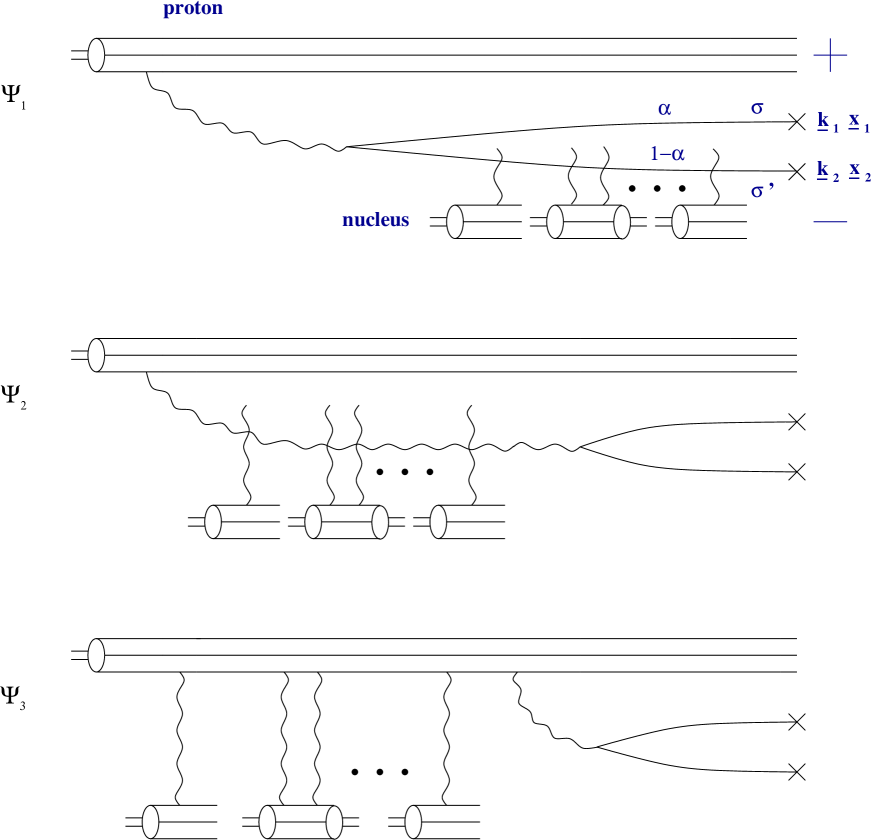
Figure 1: Three main contributions to quark-antiquark production in the quasi-classical approximation.

We begin by calculating the “wave-function” parts. In each of the diagrams in Fig. 1 they correspond to the two-step splitting $q_{v}\rightarrow q_{v}\,G\rightarrow q_{v}\,q\,\bar{q}$. However, the fact that the splittings take place either in initial or final states depending on the diagram modifies the energy denominators, making the “wave-function” parts different in all three graphs. We will denote these “wave-function” parts $\Psi_{1}$, $\Psi_{2}$ and $\Psi_{3}$ correspondingly, as shown in Fig. 1. The calculation of $\Psi_{1}$, $\Psi_{2}$ and $\Psi_{3}$ proceeds according to the rules of light cone perturbation theory (LCPT) BL in the light cone gauge of the proton, which we choose as moving in the light-cone “plus” direction (see Fig. 1). Calculations are first performed in momentum space, after which the “wave-functions” are Fourier-transformed into coordinate space.

The important subtlety of calculating final-state splittings is that the light cone denominator for such splittings should be calculated subtracting the light cone energy (the “minus” momentum component) of the outgoing final state. Indeed the light cone energies of incoming and outgoing states are equal to each other: therefore, in calculating final state splittings one can still subtract the incoming energy in the denominators. However, in doing so one has to keep track of a change in the minus component of the target’s momentum, which could be a bit tedious. For details on calculations of final state emissions in the LCPT formalism see KT ; JMK1 .

Since eikonal multiple rescatterings do not change the transverse coordinates of the incoming quarks and the gluon, we can calculate $\Psi_{1}$, $\Psi_{2}$ and $\Psi_{3}$ in transverse coordinate space by calculating the diagrams in Fig. 1 without interactions. We assume that the outgoing quark and anti-quark have momenta $k_{1}$ and $k_{2}$ correspondingly. The “plus” components of the momenta, $k_{1+}$ and $k_{2+}$ are conserved in the interactions with the target. Therefore, the “plus” component of the gluon’s momentum is equal to $k_{1+}+k_{2+}$. Here, for simplicity, we assume that $k_{1+},k_{2+}\ll p_{+}$, where $p_{+}$ is the typical light cone momentum of the valence quarks in the proton. This implies that $k_{1+}+k_{2+}\ll p_{+}$, i.e., that the gluon is also much softer than the proton. In this kinematics the “wave-functions” in momentum space are

$$\Psi^{(1)}_{\sigma,\,\sigma^{\prime}}(k_{1},k_{2}) = 2\,g\,T_{a}\,\sum_{\lambda}\,\frac{\underline{\epsilon}^{*\lambda}\cdot(\underline{k}_{1}+\underline{k}_{2})}{(\underline{k}_{1}+\underline{k}_{2})^{2}}\,g\,T_{b}\,\frac{1}{\frac{\underline{k}_{1}^{2}+m^{2}}{k_{1+}}+\frac{\underline{k}_{2}^{2}+m^{2}}{k_{2+}}}\,\frac{\bar{u}_{\sigma}(k_{1})}{\sqrt{k_{1+}}}\gamma\cdot\epsilon^{\lambda}\frac{v_{\sigma^{\prime}}(k_{2})}{\sqrt{k_{2+}}}$$ (1a)

$$- 2\,g^{2}\,T_{a}\,T_{b}\,\frac{1}{k_{1+}+k_{2+}}\,\frac{1}{\frac{\underline{k}_{1}^{2}+m^{2}}{k_{1+}}+\frac{\underline{k}_{2}^{2}+m^{2}}{k_{2+}}}\,\frac{\bar{u}_{\sigma}(k_{1})}{\sqrt{k_{1+}}}\gamma_{+}\frac{v_{\sigma^{\prime}}(k_{2})}{\sqrt{k_{2+}}}$$

$$= 2\,g\,T_{a}\,\sum_{\lambda}\,\frac{\underline{\epsilon}^{*\lambda}\cdot(\underline{k}_{1}+\underline{k}_{2})}{(\underline{k}_{1}+\underline{k}_{2})^{2}}\,g\,T_{b}\,\frac{L^{\lambda}_{\sigma,\,\sigma^{\prime}}(\underline{k}_{1}\,(1-\alpha)-\underline{k}_{2}\,\alpha;\alpha)}{{\underline{k}}_{1}^{2}\,(1-\alpha)+{\underline{k}}_{2}^{2}\,\alpha+m^{2}}\,$$

$$- 4\,g^{2}\,T_{a}\,T_{b}\,\frac{\delta_{\sigma,\,\sigma^{\prime}}\,\alpha\,(1-\alpha)}{{\underline{k}}_{1}^{2}\,(1-\alpha)+{\underline{k}}_{2}^{2}\,\alpha+m^{2}},$$

$$\Psi^{(2)}_{\sigma,\,\sigma^{\prime}}(k_{1},k_{2}) = 2\,g\,T_{a}\,\sum_{\lambda}\,\frac{\underline{\epsilon}^{*\lambda}\cdot(\underline{k}_{1}+\underline{k}_{2})}{(\underline{k}_{1}+\underline{k}_{2})^{2}}\,g\,T_{b}\,\frac{1}{\frac{(\underline{k}_{1}+\underline{k}_{2})^{2}}{k_{1+}+k_{2+}}-\frac{\underline{k}_{1}^{2}+m^{2}}{k_{1+}}-\frac{\underline{k}_{2}^{2}+m^{2}}{k_{2+}}}\,\frac{\bar{u}_{\sigma}(k_{1})}{\sqrt{k_{1+}}}\gamma\cdot\epsilon^{\lambda}\frac{v_{\sigma^{\prime}}(k_{2})}{\sqrt{k_{2+}}}$$ (1b)

$$= -2\,g\,T_{a}\,\sum_{\lambda}\,\frac{\underline{\epsilon}^{*\lambda}\cdot(\underline{k}_{1}+\underline{k}_{2})}{(\underline{k}_{1}+\underline{k}_{2})^{2}}\,g\,T_{b}\,\frac{L^{\lambda}_{\sigma,\,\sigma^{\prime}}(\underline{k}_{1}\,(1-\alpha)-\underline{k}_{2}\,\alpha;\alpha)}{[\underline{k}_{1}\,(1-\alpha)-\underline{k}_{2}\,\alpha]^{2}+m^{2}}\,,$$

$$\Psi^{(3)}_{\sigma,\,\sigma^{\prime}}(k_{1},k_{2}) = 2\,g\,T_{a}\sum_{\lambda}\frac{\underline{\epsilon}^{*\lambda}\cdot(\underline{k}_{1}+\underline{k}_{2})}{-\frac{\underline{k}_{1}^{2}+m^{2}}{k_{1+}}-\frac{\underline{k}_{2}^{2}+m^{2}}{k_{2+}}}\,g\,T_{b}\,\frac{(k_{1+}+k_{2+})^{-1}}{\frac{(\underline{k}_{1}+\underline{k}_{2})^{2}}{k_{1+}+k_{2+}}-\frac{\underline{k}_{1}^{2}+m^{2}}{k_{1+}}-\frac{\underline{k}_{2}^{2}+m^{2}}{k_{2+}}}\frac{\bar{u}_{\sigma}(k_{1})}{\sqrt{k_{1+}}}\,\gamma\cdot\epsilon^{\lambda}\frac{v_{\sigma^{\prime}}(k_{2})}{\sqrt{k_{2+}}}$$ (1c)

$$+ 2\,g^{2}\,T_{a}\,T_{b}\,\frac{1}{k_{1+}+k_{2+}}\,\frac{1}{\frac{\underline{k}_{1}^{2}+m^{2}}{k_{1+}}+\frac{\underline{k}_{2}^{2}+m^{2}}{k_{2+}}}\,\frac{\bar{u}_{\sigma}(k_{1})}{\sqrt{k_{1+}}}\gamma_{+}\frac{v_{\sigma^{\prime}}(k_{2})}{\sqrt{k_{2+}}}$$

$$= 2\,g\,T_{a}\sum_{\lambda}\frac{\underline{\epsilon}^{*\lambda}\cdot(\underline{k}_{1}+\underline{k}_{2})\,\alpha\,(1-\alpha)}{{\underline{k}}_{1}^{2}\,(1-\alpha)+{\underline{k}}_{2}^{2}\,\alpha+m^{2}}\,g\,T_{b}\,\frac{L^{\lambda}_{\sigma,\,\sigma^{\prime}}(\underline{k}_{1}\,(1-\alpha)-\underline{k}_{2}\,\alpha;\alpha)}{[\underline{k}_{1}\,(1-\alpha)-\underline{k}_{2}\,\alpha]^{2}+m^{2}}$$

$$+ 4\,g^{2}\,T_{a}\,T_{b}\,\frac{\delta_{\sigma,\,\sigma^{\prime}}\,\alpha\,(1-\alpha)}{{\underline{k}}_{1}^{2}\,(1-\alpha)+{\underline{k}}_{2}^{2}\,\alpha+m^{2}},$$

where KM

$$L^{\lambda}_{\sigma,\,\sigma^{\prime}}(\underline{k}_{1}\,(1-\alpha)-\underline{k}_{2}\,\alpha;\alpha)\,=\,-\underline{\epsilon}^{\lambda}\cdot[\underline{k}_{1}\,(1-\alpha)-\underline{k}_{2}\,\alpha]\,(1-2\,\alpha+\lambda\,\sigma)\,\delta_{\sigma,\,\sigma^{\prime}}\,-\,\frac{1}{\sqrt{2}}\,\sigma\,m\,(1-\lambda\,\sigma)\,\delta_{\sigma,-\sigma^{\prime}},$$ (2)

$\lambda=\pm 1$ is the gluon’s polarization (which also does not change under eikonal rescatterings), $\sigma=\pm 1$ and $\sigma^{\prime}=\pm 1$ are quark and anti-quark helicities correspondingly (see Fig. 1, $\sigma^{\prime}$ is defined with respect to $-\vec{k}_{2}$), $m$ is the mass of the quarks, and the colors of the gluon immediately after emission ($a$) and just before splitting into $q\bar{q}$ pair ($b$) are kept different since the color of the gluon is likely to change in interaction (for $\Psi_{2}$), due to which the color factors will be calculated separately. Gluon polarization vector for transverse gluons is given by $\epsilon_{\mu}^{\lambda}=(0,0,\underline{\epsilon}^{\lambda})$, with $\underline{\epsilon}^{\lambda}=(1+i\,\lambda)/\sqrt{2}$. The fraction of gluon’s “plus” momentum carried by the quark is denoted by $\alpha\equiv k_{1+}/(k_{1+}+k_{2+})$. The gluon ”propagators” in diagrams $\Psi_{1}$ and $\Psi_{3}$ of Fig. 1 have instantaneous (longitudinal) parts BL , which account for the second (additive) terms in Eqs. (1a) and (1c).

Note that, as can be checked explicitly using (1),

$$\Psi^{(1)}_{\sigma,\,\sigma^{\prime}}(k_{1},k_{2})+\Psi^{(2)}_{\sigma,\,\sigma^{\prime}}(k_{1},k_{2})+\Psi^{(3)}_{\sigma,\,\sigma^{\prime}}(k_{1},k_{2})\,=\,0,$$ (3)

indicating, of course, that there can be no emission without interaction.

One may worry that since the gluon in the second graph of Fig. 1 interacts with the target, and, therefore the interaction will depend on the transverse coordinate of this gluon, instead of calculating $\Psi^{(2)}_{\sigma,\,\sigma^{\prime}}(k_{1},k_{2})$ as shown above in (1b), one should separately calculate $q_{v}\rightarrow q_{v}G$ and $G\rightarrow q\,\bar{q}$ transitions in momentum space, and then separately Fourier-transform each of the results into coordinate space. However, this is not necessary, since the gluon’s transverse coordinate is uniquely fixed by the transverse coordinates of the quark $\underline{x}_{1}$ and the anti-quark $\underline{x}_{2}$ and by $\alpha$ (see e.g. KopTar ; KNST ; IKMT ). The gluon’s transverse coordinate is

$$\underline{u}\,=\,\alpha\,\underline{x}_{1}+(1-\alpha)\,\underline{x}_{2}.$$ (4)

If we perform the calculations for $q_{v}\rightarrow q_{v}G$ and $G\rightarrow q\,\bar{q}$ splittings independently, and Fourier-transform each of them into coordinate space, the $G\rightarrow q\,\bar{q}$ component will come with a delta-function $\delta^{2}(\underline{u}-\alpha\,\underline{x}_{1}+(1-\alpha)\,\underline{x}_{2})$, which vanishes after integration over $\underline{u}$ (which is an internal variable and has to be integrated over) fixing $\underline{u}$ at the value given by (4). The result of this procedure is equivalent to a simple Fourier-transform of $\Psi^{(2)}_{\sigma,\,\sigma^{\prime}}(k_{1},k_{2})$ from (1b) into coordinate space.

The light cone “wave-functions” in transverse coordinate space are defined as

$$\Psi^{(i)}_{\sigma,\,\sigma^{\prime}}(\underline{x}_{1},\underline{x}_{2};\alpha)\,=\,\int\frac{d^{2}k_{1}}{(2\pi)^{2}}\frac{d^{2}k_{2}}{(2\pi)^{2}}\,e^{-i\underline{k}_{1}\cdot\underline{x}_{1}-i\underline{k}_{2}\cdot\underline{x}_{2}}\,\Psi^{(i)}_{\sigma,\,\sigma^{\prime}}(k_{1},k_{2})\,,\quad i=1,2,3\,.$$ (5)

Here we assume that the transverse coordinate of the valence quark which emits the gluon (which splits into a $q\bar{q}$ pair) is $\underline{0}$.

To perform the Fourier transform of (5) it is convenient to introduce the following auxiliary functions

$$F_{2}(\underline{x}_{1},\underline{x}_{2};\alpha) = \int_{0}^{\infty}dq\,J_{1}(q\,u)\,K_{1}\bigg{(}x_{12}\,\sqrt{m^{2}+q^{2}\,\alpha(1-\alpha)}\bigg{)}\,\sqrt{m^{2}+q^{2}\,\alpha(1-\alpha)}\,,$$ (6)

$$F_{1}(\underline{x}_{1},\underline{x}_{2};\alpha) = \int_{0}^{\infty}dq\,J_{1}(q\,u)\,K_{0}\bigg{(}x_{12}\,\sqrt{m^{2}+q^{2}\,\alpha(1-\alpha)}\bigg{)}\,,$$ (7)

$$F_{0}(\underline{x}_{1},\underline{x}_{2};\alpha) = \int_{0}^{\infty}dq\,q\,J_{0}(q\,u)\,K_{0}\bigg{(}x_{12}\,\sqrt{m^{2}+q^{2}\,\alpha(1-\alpha)}\bigg{)}\,,$$ (8)

where $u=|\underline{u}|$, $\underline{x}_{12}=\underline{x}_{1}-\underline{x}_{2}$, $x_{12}=|\underline{x}_{12}|$, and $\underline{q}=\underline{k}_{1}+\underline{k}_{2}$. In terms of the functions defined in (6), (7) and (8) we obtain

$$\Psi^{(1)}_{\sigma,\,\sigma^{\prime}}(\underline{x}_{1},\underline{x}_{2};\alpha) = \frac{2\,g^{2}\,T_{a}\,T_{b}}{(2\pi)^{2}}\,\bigg{\{}\,\sum_{\lambda}\,\bigg{[}F_{2}(\underline{x}_{1},\underline{x}_{2};\alpha)\,\frac{\underline{x}_{12}\cdot\underline{\epsilon}^{\lambda}}{x_{12}}\,(1-2\,\alpha+\lambda\,\sigma)\,\delta_{\sigma,\sigma^{\prime}}$$

$$+ \,F_{1}(\underline{x}_{1},\underline{x}_{2};\alpha)\,\frac{i}{\sqrt{2}}\,\sigma\,m\,(1-\lambda\,\sigma)\,\delta_{\sigma,-\sigma^{\prime}}\bigg{]}\,\frac{\underline{u}\cdot\underline{\epsilon}^{*\lambda}}{u}\,$$ (9a)

$$- 2\,\delta_{\sigma,\,\sigma^{\prime}}\,\alpha\,(1-\alpha)\,F_{0}(\underline{x}_{1},\underline{x}_{2};\alpha)\,\bigg{\}},$$

$$\Psi^{(2)}_{\sigma,\,\sigma^{\prime}}(\underline{x}_{1},\underline{x}_{2};\alpha) = -\frac{2\,g^{2}\,T_{a}\,T_{b}}{(2\pi)^{2}}\,\sum_{\lambda}\,\bigg{[}\frac{\underline{x}_{12}\cdot\underline{\epsilon}^{\lambda}}{x_{12}}\,m\,K_{1}(m\,x_{12})\,(1-2\,\alpha+\lambda\,\sigma)\,\delta_{\sigma,\sigma^{\prime}}$$ (9b)

$$+\,K_{0}(m\,x_{12})\,\frac{i}{\sqrt{2}}\,\sigma\,m\,(1-\lambda\,\sigma)\,\delta_{\sigma,-\sigma^{\prime}}\bigg{]}\,\frac{\underline{u}\cdot\underline{\epsilon}^{*\lambda}}{u^{2}}\,,$$

$$\Psi^{(3)}_{\sigma,\,\sigma^{\prime}}(\underline{x}_{1},\underline{x}_{2};\alpha) = -\Psi^{(1)}_{\sigma,\,\sigma^{\prime}}(\underline{x}_{1},\underline{x}_{2};\alpha)-\Psi^{(2)}_{\sigma,\,\sigma^{\prime}}(\underline{x}_{1},\underline{x}_{2};\alpha)\,.$$ (9c)

The last relation (9c) follows from (3).

Summation over $\lambda$ yields

$$\Psi^{(1)}_{\sigma,\,\sigma^{\prime}}(\underline{x}_{1},\underline{x}_{2};\alpha) = \frac{2\,g^{2}\,T_{a}\,T_{b}}{(2\pi)^{2}}\,\bigg{[}F_{2}(\underline{x}_{1},\underline{x}_{2};\alpha)\,\frac{1}{x_{12}\,u}\,[(1-2\,\alpha)\,\underline{x}_{12}\cdot\underline{u}+i\,\sigma\,\epsilon_{ij}\,u_{i}\,x_{12\,j}]\,\delta_{\sigma,\sigma^{\prime}}$$ (10a)

$$\,+\,F_{1}(\underline{x}_{1},\underline{x}_{2};\alpha)\,\frac{i}{u}\,\sigma\,m\,(u_{x}+i\,\sigma\,u_{y})\,\delta_{\sigma,-\sigma^{\prime}}\,$$

$$- 2\,\delta_{\sigma,\,\sigma^{\prime}}\,\alpha\,(1-\alpha)\,F_{0}(\underline{x}_{1},\underline{x}_{2};\alpha)\,\bigg{]},$$

$$\Psi^{(2)}_{\sigma,\,\sigma^{\prime}}(\underline{x}_{1},\underline{x}_{2};\alpha) = -\frac{2\,g^{2}\,T_{a}\,T_{b}}{(2\pi)^{2}}\,\bigg{[}m\,K_{1}(m\,x_{12})\,\frac{1}{x_{12}\,u^{2}}\,[(1-2\,\alpha)\,\underline{x}_{12}\cdot\underline{u}+i\,\sigma\,\epsilon_{ij}\,u_{i}\,x_{12\,j}]\,\delta_{\sigma,\sigma^{\prime}}$$ (10b)

$$+\,K_{0}(m\,x_{12})\,\frac{i}{u^{2}}\,\sigma\,m\,(u_{x}+i\,\sigma\,u_{y})\,\delta_{\sigma,-\sigma^{\prime}}\bigg{]}\,,$$

$$\Psi^{(3)}_{\sigma,\,\sigma^{\prime}}(\underline{x}_{1},\underline{x}_{2};\alpha) = -\Psi^{(1)}_{\sigma,\,\sigma^{\prime}}(\underline{x}_{1},\underline{x}_{2};\alpha)-\Psi^{(2)}_{\sigma,\,\sigma^{\prime}}(\underline{x}_{1},\underline{x}_{2};\alpha)\,,$$ (10c)

where $\epsilon_{12}=1=-\epsilon_{21}$, $\epsilon_{11}=\epsilon_{22}=0$, and, assuming summation over repeating indices, $\epsilon_{ij}\,u_{i}\,v_{j}=u_{x}\,v_{y}-u_{y}\,v_{x}$. Also $x_{12\,j}$ denotes the $j$th component of the vector $\underline{x}_{12}$.

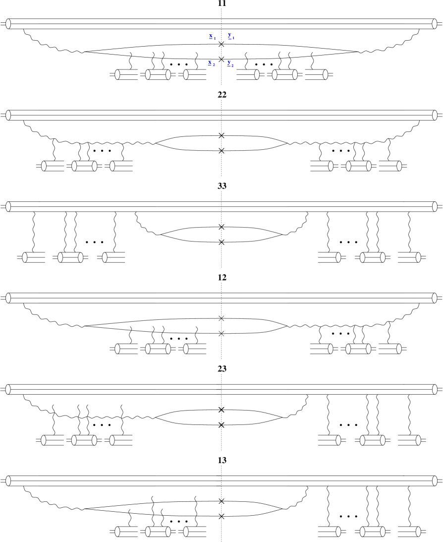
Figure 2: Diagrams contributing to quark–anti-quark pair production in the quasi-classical approximation. Disconnected $t$-channel gluon lines imply summation over all possible connections to the adjacent $s$-channel quark and gluon lines.

Now that we have calculated the “wave-functions” in (10), we can proceed by calculating the $q\bar{q}$ production cross-section. The relevant diagrams are shown in Fig. 2 and are obtained by squaring the sum of contributions from Fig. 1. We will first calculate the parts of the diagrams in Fig. 2 which are due to the squares of the “wave-functions” from (10). The resulting expressions will then be convoluted with the multiple rescattering parts of the diagrams.

The $q\bar{q}$ radiation kernel is obtained by averaging the square of the sum of the “wave functions” from (10) over the quantum numbers of the initial valence quark and summing over the quantum numbers of the final state quarks. Since we are interested, first of all, in the $q\bar{q}$ inclusive production cross section, where the transverse momenta of both the quark $\underline{k}_{1}$ and anti-quark $\underline{k}_{2}$ are fixed, in anticipation of a Fourier transform to transverse momentum space, we will keep the transverse coordinates of the quarks different in the amplitude and in the complex conjugate amplitude. Therefore, if the transverse coordinates of the quarks are $\underline{x}_{1}$ and $\underline{x}_{2}$ in the amplitude, we will denote them by $\underline{y}_{1}$ and $\underline{y}_{2}$ in the complex conjugate amplitude, as shown in the first graph of Fig. 2. The result for the squares of the “wave-functions” is

$$\Phi_{ij}(\underline{x}_{1},\underline{x}_{2};\underline{y}_{1},\underline{y}_{2};\alpha)\,=\,\frac{1}{N_{c}}\sum_{\sigma,\sigma^{\prime},a,b}\,\Psi^{(i)}_{\sigma,\,\sigma^{\prime}}(\underline{x}_{1},\underline{x}_{2};\alpha)\,\Psi^{(j)*}_{\sigma,\,\sigma^{\prime}}(\underline{y}_{1},\underline{y}_{2};\alpha)\,,\quad i,j=1,2,3\,.$$ (11)

Here the sum over gluons’ colors $a$ and $b$ simply implies a calculation of the color factors of the relevant diagrams, including traces over fermion loops. Indeed these color factors, while calculable in principle, are rather sophisticated, especially if we are interested in the double-inclusive $q\bar{q}$ production cross section. Therefore, to simplify the already quite involved calculations, we will calculate the diagrams in Fig. 2 in the large-$N_{c}$ limit. The other reason for doing this is that, even though it is clear how to improve on the large-$N_{c}$ approximation in the classical limit, inclusion of quantum evolution beyond the large-$N_{c}$ approximation would involve the functional JIMWLK JIMWLK evolution equation, a numerical solution of which is rather involved. Therefore, in the calculations of “wave-functions” squared below, the color factors will be calculated in the large-$N_{c}$ limit.

After a straightforward calculation we derive (we introduce the gluon’s transverse coordinate in the complex conjugate amplitude $\underline{v}\,\equiv\,\alpha\,\underline{y}_{1}+(1-\alpha)\,\underline{y}_{2}$ with $v=|\underline{v}|$ and $\underline{y}_{12}=\underline{y}_{1}-\underline{y}_{2}$, $y_{12}=|\underline{y}_{12}|$)

$$\Phi_{11}(\underline{x}_{1},\underline{x}_{2};\underline{y}_{1},\underline{y}_{2};\alpha)\,=\,4\,C_{F}\,\bigg{(}\frac{\alpha_{s}}{\pi}\bigg{)}^{2}\,\bigg{\{}F_{2}(\underline{x}_{1},\underline{x}_{2};\alpha)\,F_{2}(\underline{y}_{1},\underline{y}_{2};\alpha)\,\frac{1}{x_{12}\,y_{12}\,u\,v}\,[(1-2\,\alpha)^{2}$$

$$\times\,(\underline{x}_{12}\cdot\underline{u})\,(\underline{y}_{12}\cdot\underline{v})+(\epsilon_{ij}\,u_{i}\,x_{12\,j})\,(\epsilon_{kl}\,v_{k}\,y_{12\,l})]+F_{1}(\underline{x}_{1},\underline{x}_{2};\alpha)\,F_{1}(\underline{y}_{1},\underline{y}_{2};\alpha)\,m^{2}\,\frac{\underline{u}\cdot\underline{v}}{u\,v}$$

$$+4\,\alpha^{2}\,(1-\alpha)^{2}\,F_{0}(\underline{x}_{1},\underline{x}_{2};\alpha)\,F_{0}(\underline{y}_{1},\underline{y}_{2};\alpha)-2\,\alpha\,(1-\alpha)\,(1-2\,\alpha)\,\bigg{[}\frac{\underline{x}_{12}\cdot\underline{u}}{x_{12}\,u}\,F_{2}(\underline{x}_{1},\underline{x}_{2};\alpha)$$

$$\times\,F_{0}(\underline{y}_{1},\underline{y}_{2};\alpha)+\frac{\underline{y}_{12}\cdot\underline{v}}{y_{12}\,v}\,F_{2}(\underline{y}_{1},\underline{y}_{2};\alpha)\,F_{0}(\underline{x}_{1},\underline{x}_{2};\alpha)\bigg{]}\,\bigg{\}}\,,$$ (12a)

$$\Phi_{22}(\underline{x}_{1},\underline{x}_{2};\underline{y}_{1},\underline{y}_{2};\alpha)\,=\,4\,C_{F}\,\bigg{(}\frac{\alpha_{s}}{\pi}\bigg{)}^{2}\,m^{2}\,\bigg{\{}K_{1}(m\,x_{12})\,K_{1}(m\,y_{12})\,\frac{1}{x_{12}\,y_{12}\,u^{2}\,v^{2}}\,[(1-2\,\alpha)^{2}$$

$$\times\,(\underline{x}_{12}\cdot\underline{u})\,(\underline{y}_{12}\cdot\underline{v})+(\epsilon_{ij}\,u_{i}\,x_{12\,j})\,(\epsilon_{kl}\,v_{k}\,y_{12\,l})]+K_{0}(m\,x_{12})\,K_{0}(m\,y_{12})\,\frac{\underline{u}\cdot\underline{v}}{u^{2}\,v^{2}}\bigg{\}}\,,$$ (12b)

$$\Phi_{12}(\underline{x}_{1},\underline{x}_{2};\underline{y}_{1},\underline{y}_{2};\alpha)=-4\,C_{F}\,\bigg{(}\frac{\alpha_{s}}{\pi}\bigg{)}^{2}\,m\,\bigg{\{}F_{2}(\underline{x}_{1},\underline{x}_{2};\alpha)\,K_{1}(m\,y_{12})\,\frac{1}{x_{12}\,y_{12}\,u\,v^{2}}\,[(1-2\,\alpha)^{2}$$

$$\times\,(\underline{x}_{12}\cdot\underline{u})\,(\underline{y}_{12}\cdot\underline{v})+(\epsilon_{ij}\,u_{i}\,x_{12\,j})\,(\epsilon_{kl}\,v_{k}\,y_{12\,l})]+m\,F_{1}(\underline{x}_{1},\underline{x}_{2};\alpha)\,K_{0}(m\,y_{12})\,\frac{\underline{u}\cdot\underline{v}}{u\,v^{2}}$$

$$-2\,\alpha\,(1-\alpha)\,(1-2\,\alpha)\,\frac{\underline{y}_{12}\cdot\underline{v}}{y_{12}\,v^{2}}\,F_{0}(\underline{x}_{1},\underline{x}_{2};\alpha)\,K_{1}(m\,y_{12})\bigg{\}}\,,$$ (12c)

$$\Phi_{33}(\underline{x}_{1},\underline{x}_{2};\underline{y}_{1},\underline{y}_{2};\alpha)\,=\,\Phi_{11}(\underline{x}_{1},\underline{x}_{2};\underline{y}_{1},\underline{y}_{2};\alpha)+\Phi_{22}(\underline{x}_{1},\underline{x}_{2};\underline{y}_{1},\underline{y}_{2};\alpha)+\Phi_{12}(\underline{x}_{1},\underline{x}_{2};\underline{y}_{1},\underline{y}_{2};\alpha)$$

$$+\Phi_{21}(\underline{x}_{1},\underline{x}_{2};\underline{y}_{1},\underline{y}_{2};\alpha)$$ (12d)

$$\Phi_{13}(\underline{x}_{1},\underline{x}_{2};\underline{y}_{1},\underline{y}_{2};\alpha)\,=\,-\Phi_{11}(\underline{x}_{1},\underline{x}_{2};\underline{y}_{1},\underline{y}_{2};\alpha)-\Phi_{12}(\underline{x}_{1},\underline{x}_{2};\underline{y}_{1},\underline{y}_{2};\alpha)$$ (12e)

$$\Phi_{23}(\underline{x}_{1},\underline{x}_{2};\underline{y}_{1},\underline{y}_{2};\alpha)\,=\,-\Phi_{21}(\underline{x}_{1},\underline{x}_{2};\underline{y}_{1},\underline{y}_{2};\alpha)-\Phi_{22}(\underline{x}_{1},\underline{x}_{2};\underline{y}_{1},\underline{y}_{2};\alpha)$$ (12f)

$$\Phi_{ij}(\underline{x}_{1},\underline{x}_{2};\underline{y}_{1},\underline{y}_{2};\alpha)\,=\,\Phi_{ji}^{*}(\underline{y}_{1},\underline{y}_{2};\underline{x}_{1},\underline{x}_{2};\alpha).$$ (12g)

Here Eqs. (12d,12e,12f) follow from (10c). (12g) allows one to obtain $\Phi_{21}$, $\Phi_{31}$ and $\Phi_{32}$ from (12c), (12e) and (12f).

Rescattering of $q_{v}$, $q_{v}\,G$ and $q_{v}\,q\,\bar{q}$ configurations on a large nucleus brings in different factors, which we label $\Xi_{ij}$ depending on the diagram shown in Fig. 2. For the case of single-quark inclusive production cross section (when transverse momentum of one of the quarks is integrated over) they were calculated in Tuchin:2004rb . As we mentioned above, the calculations complicate tremendously for the double-inclusive $q\bar{q}$ production cross section we are interested in calculating here. We will, therefore, perform our calculations on the large-$N_{c}$ limit. Introducing quark saturation scale KM ; JMK

$$Q_{s}^{2}\,=\,\frac{4\,\pi\,\alpha_{s}^{2}\,C_{F}}{N_{c}}\,\rho\,T(\underline{b})\,\approx\,2\,\pi\,\alpha_{s}^{2}\,N_{c}\,\rho\,T(\underline{b})$$ (13)

with $\rho$ the nucleon number density in the nucleus and $T(\underline{b})$ the nuclear profile function, we write

$$\Xi_{11}(\underline{x}_{1},\underline{x}_{2};\underline{y}_{1},\underline{y}_{2};\alpha) = e^{-\frac{1}{4}\,(\underline{x}_{1}-\underline{y}_{1})^{2}\,Q_{s}^{2}\,\ln(1/|\underline{x}_{1}-\underline{y}_{1}|\,\Lambda)-\frac{1}{4}\,(\underline{x}_{2}-\underline{y}_{2})^{2}\,Q_{s}^{2}\,\ln(1/|\underline{x}_{2}-\underline{y}_{2}|\,\Lambda)}\,,$$ (14a)

$$\Xi_{22}(\underline{x}_{1},\underline{x}_{2};\underline{y}_{1},\underline{y}_{2};\alpha) = e^{-\frac{1}{2}\,(\underline{u}-\underline{v})^{2}\,Q_{s}^{2}\,\ln(1/|\underline{u}-\underline{v}|\,\Lambda)}\,,$$ (14b)

$$\Xi_{33}(\underline{x}_{1},\underline{x}_{2};\underline{y}_{1},\underline{y}_{2};\alpha) = 1\,,$$ (14c)

$$\Xi_{12}(\underline{x}_{1},\underline{x}_{2};\underline{y}_{1},\underline{y}_{2};\alpha) = e^{-\frac{1}{4}\,(\underline{x}_{1}-\underline{v})^{2}\,Q_{s}^{2}\,\ln(1/|\underline{x}_{1}-\underline{v}|\,\Lambda)-\frac{1}{4}\,(\underline{x}_{2}-\underline{v})^{2}\,Q_{s}^{2}\,\ln(1/|\underline{x}_{2}-\underline{v}|\,\Lambda)}\,,$$ (14d)

$$\Xi_{23}(\underline{x}_{1},\underline{x}_{2};\underline{y}_{1},\underline{y}_{2};\alpha) = e^{-\frac{1}{2}\,u^{2}\,Q_{s}^{2}\,\ln(1/u\,\Lambda)}\,,$$ (14e)

$$\Xi_{13}(\underline{x}_{1},\underline{x}_{2};\underline{y}_{1},\underline{y}_{2};\alpha) = e^{-\frac{1}{4}\,x_{1}^{2}\,Q_{s}^{2}\,\ln(1/x_{1}\Lambda)-\frac{1}{4}\,x_{2}^{2}\,Q_{s}^{2}\,\ln(1/x_{2}\Lambda)}\,$$ (14f)

with $\Lambda$ some infrared cutoff. All other $\Xi_{ij}$’s can be found from the components listed in (14) using

$$\Xi_{ij}(\underline{x}_{1},\underline{x}_{2};\underline{y}_{1},\underline{y}_{2};\alpha)\,=\,\Xi_{ji}(\underline{y}_{1},\underline{y}_{2};\underline{x}_{1},\underline{x}_{2};\alpha)$$ (15)

similar to (12g). Note that in arriving at equations (14) we have used the fact that the valence quark rescatterings on the target cancel due to real-virtual cancellations in the first four graphs in Fig. 2 KoM . Such cancellations do not happen completely for a projectile dipole, as we will see in Section III.

Using Eqs. (12) and (14) we derive the double-inclusive quark–anti-quark production cross section in $pA$ collisions in the quasi-classical approximation

$$\frac{d\,\sigma}{d^{2}k_{1}\,d^{2}k_{2}\,dy\,d\alpha\,d^{2}b}\,=\,\frac{1}{4\,(2\,\pi)^{6}}\,\int d^{2}x_{1}\,d^{2}x_{2}\,d^{2}y_{1}\,d^{2}y_{2}\,e^{-i\,\underline{k}_{1}\cdot(\underline{x}_{1}-\underline{y}_{1})-i\,\underline{k}_{2}\cdot(\underline{x}_{2}-\underline{y}_{2})}$$

$$\times\,\sum_{i,j=1}^{3}\,\Phi_{ij}(\underline{x}_{1},\underline{x}_{2};\underline{y}_{1},\underline{y}_{2};\alpha)\ \Xi_{ij}(\underline{x}_{1},\underline{x}_{2};\underline{y}_{1},\underline{y}_{2};\alpha).$$ (16)

Here $y$ is the rapidity of the $s$-channel gluon, which splits into the $q\bar{q}$ pair. Since the quark and the anti-quark are most likely to be produced close to each other in rapidity, one can think of $y$ as the rapidity of the quarks. $\underline{b}$ is the impact parameter of the proton with respect to the nucleus.

The single inclusive quark production cross section is easily obtained from (16) by integrating over one of the quark’s momenta

$$\frac{d\,\sigma}{d^{2}k\,dy\,d^{2}b}\,=\,\frac{1}{2\,(2\,\pi)^{4}}\,\int d^{2}x_{1}\,d^{2}x_{2}\,d^{2}y_{1}\,\int_{0}^{1}d\alpha\,e^{-i\,\underline{k}\cdot(\underline{x}_{1}-\underline{y}_{1})}\,\sum_{i,j=1}^{3}\,\Phi_{ij}\,(\underline{x}_{1},\underline{x}_{2};\underline{y}_{1},\underline{x}_{2};\alpha)$$

$$\times\,\Xi_{ij}(\underline{x}_{1},\underline{x}_{2};\underline{y}_{1},\underline{x}_{2};\alpha)\,,$$ (17)

where we inserted an overall factor of $2$ to account for both quarks and anti-quarks. In (17) $y$ is the rapidity of the produced (anti-)quark.

III Including Quantum Evolution

Here we are going to include small-$x$ nonlinear quantum evolution of BK into the cross sections from Eqs. (16) and (17). Since the evolution equations in BK are written for the forward amplitude of a quark dipole on a nucleus, we have to first generalize (16) to the case of $q\bar{q}$ production in dipole-nucleus scattering. Indeed, strictly speaking our results would then only be applicable to particle production in deep inelastic scattering. However, our results below may still serve as a good approximation for gluon production in $pA$ collisions KT . The generalization of Eqs. (16) and (17) to dipole-nucleus scattering is easily done by including emissions of the $s$-channel gluon in Fig. 2 by the quark and anti-quark in the incoming dipole. If the transverse coordinates of the quark and anti-quark in the incoming dipole are denoted by $\underline{z}_{0}$ and $\underline{z}_{1}$ correspondingly with $\underline{z}_{01}=\underline{z}_{0}-\underline{z}_{1}$, we write

$$\frac{d\,\sigma}{d^{2}k_{1}\,d^{2}k_{2}\,dy\,d\alpha\,d^{2}b}(\underline{z}_{01})\,=\,\frac{1}{4\,(2\,\pi)^{6}}\,\int d^{2}x_{1}\,d^{2}x_{2}\,d^{2}y_{1}\,d^{2}y_{2}\,e^{-i\,\underline{k}_{1}\cdot(\underline{x}_{1}-\underline{y}_{1})-i\,\underline{k}_{2}\cdot(\underline{x}_{2}-\underline{y}_{2})}$$

$$\times\,\sum_{i,j=1}^{3}\,\sum_{k,l=0}^{1}\,(-1)^{k+l}\,\Phi_{ij}(\underline{x}_{1}-\underline{z}_{k},\underline{x}_{2}-\underline{z}_{k};\underline{y}_{1}-\underline{z}_{l},\underline{y}_{2}-\underline{z}_{l};\alpha)\ \Xi_{ij}(\underline{x}_{1},\underline{x}_{2},\underline{z}_{k};\underline{y}_{1},\underline{y}_{2},\underline{z}_{l};\alpha),$$ (18)

where now we have

$$\Xi_{11}(\underline{x}_{1},\underline{x}_{2},\underline{z}_{k};\underline{y}_{1},\underline{y}_{2},\underline{z}_{l};\alpha) = e^{-\frac{1}{4}\,(\underline{x}_{1}-\underline{y}_{1})^{2}\,Q_{s}^{2}\,\ln(1/|\underline{x}_{1}-\underline{y}_{1}|\,\Lambda)-\frac{1}{4}\,(\underline{x}_{2}-\underline{y}_{2})^{2}\,Q_{s}^{2}\,\ln(1/|\underline{x}_{2}-\underline{y}_{2}|\,\Lambda)}\,,$$ (19a)

$$\Xi_{22}(\underline{x}_{1},\underline{x}_{2},\underline{z}_{k};\underline{y}_{1},\underline{y}_{2},\underline{z}_{l};\alpha) = e^{-\frac{1}{2}\,(\underline{u}-\underline{v})^{2}\,Q_{s}^{2}\,\ln(1/|\underline{u}-\underline{v}|\,\Lambda)}\,,$$ (19b)

$$\Xi_{33}(\underline{x}_{1},\underline{x}_{2},\underline{z}_{k};\underline{y}_{1},\underline{y}_{2},\underline{z}_{l};\alpha) = e^{-\frac{1}{2}z_{kl}^{2}Q_{s}^{2}\,\ln(1/z_{kl}\,\Lambda)}\,,$$ (19c)

$$\Xi_{12}(\underline{x}_{1},\underline{x}_{2},\underline{z}_{k};\underline{y}_{1},\underline{y}_{2},\underline{z}_{l};\alpha) = e^{-\frac{1}{4}\,(\underline{x}_{1}-\underline{v})^{2}\,Q_{s}^{2}\,\ln(1/|\underline{x}_{1}-\underline{v}|\,\Lambda)-\frac{1}{4}\,(\underline{x}_{2}-\underline{v})^{2}\,Q_{s}^{2}\,\ln(1/|\underline{x}_{2}-\underline{v}|\,\Lambda)}\,,$$ (19d)

$$\Xi_{23}(\underline{x}_{1},\underline{x}_{2},\underline{z}_{k};\underline{y}_{1},\underline{y}_{2},\underline{z}_{l};\alpha) = e^{-\frac{1}{2}\,(\underline{u}-\underline{z}_{l})^{2}\,Q_{s}^{2}\,\ln(1/|\underline{u}-\underline{z}_{l}|\,\Lambda)}\,,$$ (19e)

$$\Xi_{13}(\underline{x}_{1},\underline{x}_{2},\underline{z}_{k};\underline{y}_{1},\underline{y}_{2},\underline{z}_{l};\alpha) = e^{-\frac{1}{4}\,(\underline{x}_{1}-\underline{z}_{l})^{2}\,Q_{s}^{2}\,\ln(1/|\underline{x}_{1}-\underline{z}_{l}|\,\Lambda)-\frac{1}{4}\,(\underline{x}_{2}-\underline{z}_{l})^{2}\,Q_{s}^{2}\,\ln(1/|\underline{x}_{2}-\underline{z}_{l}|\,\Lambda)}\,.$$ (19f)

Again, all other $\Xi_{ij}$’s can be found from the components listed in (19) using

$$\Xi_{ij}(\underline{x}_{1},\underline{x}_{2},\underline{z}_{k};\underline{y}_{1},\underline{y}_{2},\underline{z}_{l};\alpha)\,=\,\Xi_{ji}(\underline{y}_{1},\underline{y}_{2},\underline{z}_{l};\underline{x}_{1},\underline{x}_{2},\underline{z}_{k};\alpha).$$ (20)

The inclusion of quantum corrections due to leading logarithmic (resumming powers of $\alpha_{s}\,y$) approximation in the large-$N_{c}$ limit is done along the lines of KT (see also JMK1 ; Marquet ; yuri05 and JMK for a review) using Mueller’s dipole model formalism dipole . Since the integration over rapidity interval separating the quark and the anti-quark in the pair does not generate a factor of the total rapidity interval $Y$ of the collision (i.e., does not give a leading logarithm of energy), the prescription for inclusion of quantum evolution is identical to the single gluon production case. We first define the quantity $n_{1}({\underline{z}}_{0},\underline{z}_{1};{\underline{w}}_{0},\underline{w}_{1};Y-y)$, which has the meaning of the number of dipoles with transverse coordinates ${\underline{w}}_{0},\underline{w}_{1}$ at rapidity $y$ generated by the evolution from the original dipole ${\underline{z}}_{0},\underline{z}_{1}$ having rapidity $Y$. It obeys the dipole equivalent of the BFKL evolution equation dipole ; BFKL

$$\frac{\partial n_{1}({\underline{z}}_{0},\underline{z}_{1};{\underline{w}}_{0},\underline{w}_{1};y)}{\partial y}\,=\,\frac{\alpha_{s}\,N_{c}}{2\,\pi^{2}}\,\int d^{2}z_{2}\,\frac{z_{01}^{2}}{z_{20}^{2}\,z_{21}^{2}}\,\bigg{[}n_{1}({\underline{z}}_{0},\underline{z}_{2};{\underline{w}}_{0},\underline{w}_{1};y)+n_{1}({\underline{z}}_{2},\underline{z}_{1};{\underline{w}}_{0},\underline{w}_{1};y)$$

$$-n_{1}({\underline{z}}_{0},\underline{z}_{1};{\underline{w}}_{0},\underline{w}_{1};y)\bigg{]}$$ (21)

with the initial condition

$$n_{1}({\underline{z}}_{0},\underline{z}_{1};{\underline{w}}_{0},\underline{w}_{1};y=0)\,=\,\delta(\underline{z}_{0}-\underline{w}_{0})\,\delta(\underline{z}_{1}-\underline{w}_{1}).$$ (22)

If the target nucleus has rapidity $0$, the incoming dipole has rapidity $Y$, and the produced quarks have rapidity $y$, the inclusion of small-$x$ evolution in the rapidity interval $Y-y$ is accomplished by replacing the cross section from (18) by KT ; Marquet ; JMK

$$\frac{d\,\sigma}{d^{2}k_{1}\,d^{2}k_{2}\,dy\,d\alpha\,d^{2}b}(\underline{z}_{01})\rightarrow\int d^{2}w_{0}\,d^{2}w_{1}\,n_{1}({\underline{z}}_{0},\underline{z}_{1};{\underline{w}}_{0},\underline{w}_{1};Y-y)\,\frac{d\,\sigma}{d^{2}k_{1}\,d^{2}k_{2}\,dy\,d\alpha\,d^{2}b}(\underline{w}_{01}).$$ (23)

Note that while the substitution in (23) includes only linear evolution, it results from analyzing all the possible non-linear evolution corrections including all possible pomeron splittings between the projectile and the produced $q\bar{q}$ pair. As was originally shown in KT the pomeron splittings cancel in the rapidity interval between $y$ and $Y$, leaving only the linear evolution contribution included in (23).

Inclusion of evolution in the interval between $0$ and $y$ is accomplished by replacing the Mueller-Glauber rescattering exponents according to the following rule KT

$$e^{-\frac{1}{4}\,(\underline{x}_{0}-\underline{x}_{1})^{2}\,Q_{s}^{2}\,\ln(1/|\underline{x}_{0}-\underline{x}_{1}|\,\Lambda)}\,\rightarrow\,1-N(\underline{x}_{0},\underline{x}_{1},Y)$$ (24)

where $N(\underline{x}_{0},\underline{x}_{1},Y)$ is the forward amplitude for a quark dipole $\underline{x}_{0},\underline{x}_{1}$ scattering on a target with rapidity interval $Y$ between the dipole and the target. It obeys the following evolution equation BK

$$\frac{\partial N({\underline{x}}_{0},{\underline{x}}_{1},Y)}{\partial Y}\,=\,\frac{\alpha_{s}\,N_{c}}{2\,\pi^{2}}\,\int d^{2}x_{2}\,\frac{x_{01}^{2}}{x_{20}^{2}\,x_{21}^{2}}\,\left[N({\underline{x}}_{0},{\underline{x}}_{2},Y)+N({\underline{x}}_{2},{\underline{x}}_{1},Y)-N({\underline{x}}_{0},{\underline{x}}_{1},Y)\right.$$

$$-\left.N({\underline{x}}_{0},{\underline{x}}_{2},Y)\,N({\underline{x}}_{2},{\underline{x}}_{1},Y)\right]$$ (25)

with the initial condition

$$N({\underline{x}}_{0},{\underline{x}}_{1},Y=0)\,=\,1-e^{-\frac{1}{4}\,(\underline{x}_{0}-\underline{x}_{1})^{2}\,Q_{s}^{2}\,\ln(1/|\underline{x}_{0}-\underline{x}_{1}|\,\Lambda)}.$$ (26)

Performing the substitution from (24) in (19) yields

$$\Xi_{11}(\underline{x}_{1},\underline{x}_{2},\underline{z}_{k};\underline{y}_{1},\underline{y}_{2},\underline{z}_{l};\alpha,Y) = -N(\underline{x}_{1},\underline{y}_{1},Y)-N(\underline{x}_{2},\underline{y}_{2},Y)$$ (27a)

$$+N(\underline{x}_{1},\underline{y}_{1},Y)\,N(\underline{x}_{2},\underline{y}_{2},Y)\,,$$

$$\Xi_{22}(\underline{x}_{1},\underline{x}_{2},\underline{z}_{k};\underline{y}_{1},\underline{y}_{2},\underline{z}_{l};\alpha,Y) = -2\,N(\underline{u},\underline{v},Y)+N(\underline{u},\underline{v},Y)^{2}\,,$$ (27b)

$$\Xi_{33}(\underline{x}_{1},\underline{x}_{2},\underline{z}_{k};\underline{y}_{1},\underline{y}_{2},\underline{z}_{l};\alpha,Y) = -2\,N(\underline{z}_{k},\underline{z}_{l},Y)+N(\underline{z}_{k},\underline{z}_{l},Y)^{2}\,,$$ (27c)

$$\Xi_{12}(\underline{x}_{1},\underline{x}_{2},\underline{z}_{k};\underline{y}_{1},\underline{y}_{2},\underline{z}_{l};\alpha,Y) = -N(\underline{x}_{1},\underline{v},Y)-N(\underline{x}_{2},\underline{v},Y)$$ (27d)

$$+N(\underline{x}_{1},\underline{v},Y)\,N(\underline{x}_{2},\underline{v},Y)\,,$$

$$\Xi_{23}(\underline{x}_{1},\underline{x}_{2},\underline{z}_{k};\underline{y}_{1},\underline{y}_{2},\underline{z}_{l};\alpha,Y) = -2\,N(\underline{u},\underline{z}_{l},Y)+N(\underline{u},\underline{z}_{l},Y)^{2}\,,$$ (27e)

$$\Xi_{13}(\underline{x}_{1},\underline{x}_{2},\underline{z}_{k};\underline{y}_{1},\underline{y}_{2},\underline{z}_{l};\alpha,Y) = -N(\underline{x}_{1},\underline{z}_{l},Y)-N(\underline{x}_{2},\underline{z}_{l},Y)$$ (27f)

$$+N(\underline{x}_{1},\underline{z}_{l},Y)\,N(\underline{x}_{2},\underline{z}_{l},Y)\,,$$

with

$$\Xi_{ij}(\underline{x}_{1},\underline{x}_{2},\underline{z}_{k};\underline{y}_{1},\underline{y}_{2},\underline{z}_{l};\alpha,Y)\,=\,\Xi_{ji}(\underline{y}_{1},\underline{y}_{2},\underline{z}_{l};\underline{x}_{1},\underline{x}_{2},\underline{z}_{k};\alpha,Y).$$ (28)

In arriving at (27) we have dropped additive unit terms which do not contribute to the cross-section due to (3) leading to $\sum_{ij=1}^{3}\Phi_{ij}=0$.

With the definition of Eqs. (27) we write the following answer for the double inclusive $q\bar{q}$ production cross section including small-$x$ evolution effects

$$\frac{d\,\sigma}{d^{2}k_{1}\,d^{2}k_{2}\,dy\,d\alpha\,d^{2}b}(\underline{z}_{01})\,=\,\frac{1}{4\,(2\,\pi)^{6}}\,\int d^{2}w_{0}\,d^{2}w_{1}\,n_{1}({\underline{z}}_{0},\underline{z}_{1};{\underline{w}}_{0},\underline{w}_{1};Y-y)\,$$

$$\times\,d^{2}x_{1}\,d^{2}x_{2}\,d^{2}y_{1}\,d^{2}y_{2}\,e^{-i\,\underline{k}_{1}\cdot(\underline{x}_{1}-\underline{y}_{1})-i\,\underline{k}_{2}\cdot(\underline{x}_{2}-\underline{y}_{2})}$$

$$\times\,\sum_{i,j=1}^{3}\,\sum_{k,l=0}^{1}\,(-1)^{k+l}\,\Phi_{ij}(\underline{x}_{1}-\underline{w}_{k},\underline{x}_{2}-\underline{w}_{k};\underline{y}_{1}-\underline{w}_{l},\underline{y}_{2}-\underline{w}_{l};\alpha)\ \Xi_{ij}(\underline{x}_{1},\underline{x}_{2},\underline{w}_{k};\underline{y}_{1},\underline{y}_{2},\underline{w}_{l};\alpha,y).$$ (29)

Similar to how we arrived at (17), we integrate over one of the quarks’ transverse momenta to obtain the single inclusive quark production cross section

$$\frac{d\,\sigma}{d^{2}k\,\,dy\,d^{2}b}(\underline{z}_{01})\,=\,\frac{1}{2\,(2\,\pi)^{4}}\,\int d^{2}w_{0}\,d^{2}w_{1}\,n_{1}({\underline{z}}_{0},\underline{z}_{1};{\underline{w}}_{0},\underline{w}_{1};Y-y)\,d^{2}x_{1}\,d^{2}x_{2}\,d^{2}y_{1}\,e^{-i\,\underline{k}\cdot(\underline{x}_{1}-\underline{y}_{1})}$$

$$\times\int_{0}^{1}d\alpha\sum_{i,j=1}^{3}\sum_{k,l=0}^{1}(-1)^{k+l}\,\Phi_{ij}(\underline{x}_{1}-\underline{w}_{k},\underline{x}_{2}-\underline{w}_{k};\underline{y}_{1}-\underline{w}_{l},\underline{x}_{2}-\underline{w}_{l};\alpha)\ \Xi_{ij}(\underline{x}_{1},\underline{x}_{2},\underline{w}_{k};\underline{y}_{1},\underline{x}_{2},\underline{w}_{l};\alpha,y).$$ (30)

Equations (29) and (30) are the central results of this paper.

An example of the pomeron fan diagram contributing to the obtained cross sections is shown in Fig. 3. There the proton or $q\bar{q}$ dipole in DIS is shown on top of the figure. The nucleus is represented by the straight lines at the bottom of the figure. As usual each ladder represents a BFKL pomeron. Fig. 3 reflects the main features of equations (29) and (30): it contains a linear evolution between the produced $q\bar{q}$ pair and the projectile, and the non-linear evolution between the $q\bar{q}$ pair and the target. Indeed a relatively simple diagram in Fig. 3 does not include all the complexity of the nonlinear interactions in (27) and of the emission wave functions in (12).

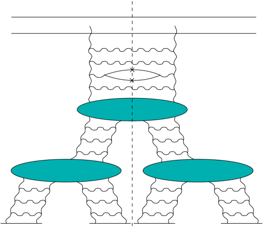
Figure 3: An example of a pomeron fan diagram contributing to the $q\bar{q}$ production cross section in proton-nucleus collisions or in DIS as calculated in equations (29) and (30). The produced quark and anti-quark are marked by crosses.

IV Summary

Expressions (29) and (30) for the single and double inclusive quark production have been derived by summing perturbation series in the coupling constant $\alpha_{s}$. In that sense our result is perturbative. It was pointed out in Kharzeev:2005iz ; Kharzeev:2006zm ; Gelis:2005gs that there can be a significant non-perturbative contribution to particle production in high energy QCD. The investigation of this effect is beyond the scope of the present paper: however it certainly deserves further study.

Equations (29) and (30) have important phenomenological applications for studying the dense partonic system in p(d)A and eA collisions. Observation of hadron suppression in the nuclear modification factor measured in dA collisions at forward rapidities at Relativistic Heavy Ion Collider (RHIC) dAdata signals the onset of the nonlinear evolution of the scattering amplitude for light hadrons KLM ; Kharzeev:2003wz ; KW . Due to a large mass, the impact of nonlinear evolution effects on the heavy quark production is shifted to higher energy and/or rapidity. It was estimated in KhT using the $k_{T}$-factorization approach that one can expect a significant deviation of the open charm production cross section from the perturbative behavior already at pseudo-rapidity $\eta\simeq 2$ at RHIC. Due to the heavy quark production threshold one expects that the total multiplicity of open charm scales as $N_{\mathrm{coll}}$ at lower energy and/or rapidity whereas at higher energies and/or rapidities the scaling law should coincide with that for lighter hadrons KhT , i. e. open charm multiplicity should scale as $N_{\mathrm{part}}$ KL due to high parton density effects. Therefore, to be able to compare predictions of CGC with the data reported by RHIC experiments and to make predictions for the possible upcoming $pA$ run at the Large Hadron Collider (LHC), it is important to perform a calculation of an open charm production within the more general approach developed in this paper. Our final results (29) and (30) allow one to describe open charm transverse momentum spectra at different rapidities and center-of-mass energies, allowing for a complete description of RHIC and LHC data. Since the saturation scale $Q_{s}$ is expected to be even higher at LHC than it was at RHIC, the CGC effects on heavy quark production at LHC should be even more significant.

Acknowledgments

The work of Yu. K. is supported in part by the U.S. Department of Energy under Grant No. DE-FG02-05ER41377. K. T. would like to thank RIKEN, BNL and the U.S. Department of Energy (Contract No. DE-AC02-98CH10886) for providing the facilities essential for the completion of this work.

References

• (1) K. Tuchin, Phys. Lett. B 593, 66 (2004) [arXiv:hep-ph/0401022].
• (2) J. P. Blaizot, F. Gelis and R. Venugopalan, Nucl. Phys. A 743, 57 (2004) [arXiv:hep-ph/0402257].
• (3) T. Appelquist and J. Carazzone, Phys. Rev. D 11, 2856 (1975).
• (4) P. Nason, S. Dawson and R. K. Ellis, Nucl. Phys. B 327, 49 (1989) [Erratum-ibid. B 335, 260 (1990)]; P. Nason, S. Dawson and R. K. Ellis, Nucl. Phys. B 303, 607 (1988).
• (5) N. Brambilla et al., arXiv:hep-ph/0412158.
• (6) L. V. Gribov, E. M.  and M. G. Ryskin, Phys. Rept.  100, 1 (1983).
• (7) A. H. Mueller and J. w. Qiu, Nucl. Phys. B 268, 427 (1986).
• (8) J. P. Blaizot and A. H. Mueller, Nucl. Phys. B 289, 847 (1987).
• (9) L. D. McLerran and R. Venugopalan, Phys. Rev. D 49, 2233 (1994) [arXiv:hep-ph/9309289], Phys. Rev. D 49, 3352 (1994) [arXiv:hep-ph/9311205], Phys. Rev. D 50, 2225 (1994) [arXiv:hep-ph/9402335], Phys. Rev. D 59, 094002 (1999) [arXiv:hep-ph/9809427]. A. Ayala, J. Jalilian-Marian, L. D. McLerran and R. Venugopalan, Phys. Rev. D 53, 458 (1996) [arXiv:hep-ph/9508302].
• (10) E. Iancu and R. Venugopalan, arXiv:hep-ph/0303204.
• (11) H. Weigert, Prog. Part. Nucl. Phys.  55, 461 (2005) [arXiv:hep-ph/0501087].
• (12) E. M. Levin, M. G. Ryskin, Y. M. Shabelski and A. G. Shuvaev, Sov. J. Nucl. Phys.  53, 657 (1991) [Yad. Fiz.  53, 1059 (1991)]. M. G. Ryskin, Y. M. Shabelski and A. G. Shuvaev, Z. Phys. C 69, 269 (1996) [Yad. Fiz.  59, 521 (1996 PANUE,59,493-500.1996)] [arXiv:hep-ph/9506338].
• (13) S. Catani, M. Ciafaloni and F. Hautmann, Nucl. Phys. B 366, 135 (1991).
• (14) J. C. Collins and R. K. Ellis, Nucl. Phys. B 360, 3 (1991).
• (15) H. Fujii, F. Gelis and R. Venugopalan, Phys. Rev. Lett.  95, 162002 (2005) [arXiv:hep-ph/0504047].
• (16) Y. V. Kovchegov and K. Tuchin, Phys. Rev. D 65, 074026 (2002) [arXiv:hep-ph/0111362].
• (17) J. Jalilian-Marian and Y. V. Kovchegov, Phys. Rev. D 70, 114017 (2004) [Erratum-ibid. D 71, 079901 (2005)] [arXiv:hep-ph/0405266].
• (18) F. Gelis and R. Venugopalan, Phys. Rev. D 69, 014019 (2004) [arXiv:hep-ph/0310090].
• (19) D. Kharzeev and K. Tuchin, arXiv:hep-ph/0310358.
• (20) B. Z. Kopeliovich and A. V. Tarasov, Nucl. Phys. A 710, 180 (2002) [arXiv:hep-ph/0205151].
• (21) F. Gelis, K. Kajantie and T. Lappi, Phys. Rev. C 71, 024904 (2005) [arXiv:hep-ph/0409058].
• (22) Y. V. Kovchegov and A. H. Mueller, Nucl. Phys. B 529, 451 (1998) [arXiv:hep-ph/9802440].
• (23) Y. V. Kovchegov and L. D. McLerran, Phys. Rev. D 60, 054025 (1999) [Erratum-ibid. D 62, 019901 (2000)] [arXiv:hep-ph/9903246].
• (24) J. Jalilian-Marian and Y. V. Kovchegov, Prog. Part. Nucl. Phys.  56, 104 (2006) [arXiv:hep-ph/0505052].
• (25) G. P. Lepage and S. J. Brodsky, Phys. Rev. D 22, 2157 (1980).
• (26) J. Jalilian-Marian, A. Kovner, A. Leonidov and H. Weigert, Phys. Rev.  D59 (1999) 014014 [arXiv:hep-ph/9706377];   Nucl. Phys. B504 (1997) 415 [arXiv:hep-ph/9701284];
E. Iancu, A. Leonidov and L. D. McLerran, Phys. Lett.  B510 (2001) 133 [arXiv:hep-ph/0102009];   Nucl. Phys.  A692 (2001) 583 [arXiv:hep-ph/0011241];
H. Weigert, Nucl. Phys.  A703 (2002) 823 [arXiv:hep-ph/0004044].
• (27) B. Z. Kopeliovich, J. Nemchik, A. Schafer and A. V. Tarasov, Phys. Rev. Lett.  88, 232303 (2002) [arXiv:hep-ph/0201010].
• (28) K. Itakura, Y. V. Kovchegov, L. McLerran and D. Teaney, Nucl. Phys. A 730, 160 (2004) [arXiv:hep-ph/0305332].
• (29) I. Balitsky, Nucl. Phys. B 463, 99 (1996) [arXiv:hep-ph/9509348]; Y. V. Kovchegov, Phys. Rev. D 60, 034008 (1999) [arXiv:hep-ph/9901281].
• (30) C. Marquet, Nucl. Phys. B 705, 319 (2005) [arXiv:hep-ph/0409023].
• (31) Y. V. Kovchegov, Phys. Rev. D 72, 094009 (2005) [arXiv:hep-ph/0508276].
• (32) A. H. Mueller, Nucl. Phys. B 335, 115 (1990); Nucl. Phys. B 415, 373 (1994); A. H. Mueller and B. Patel, Nucl. Phys. B 425, 471 (1994) [arXiv:hep-ph/9403256]; A. H. Mueller, Nucl. Phys. B 437, 107 (1995) [arXiv:hep-ph/9408245].
• (33) E. A. Kuraev, L. N. Lipatov and V. S. Fadin, Sov. Phys. JETP 45, 199 (1977) [Zh. Eksp. Teor. Fiz.  72, 377 (1977)]. I. I. Balitsky and L. N. Lipatov, Sov. J. Nucl. Phys.  28, 822 (1978) [Yad. Fiz.  28, 1597 (1978)].
• (34) I. Arsene et al. [BRAHMS Collaboration], Phys. Rev. Lett.  91, 072305 (2003) [arXiv:nucl-ex/0307003]; S. S. Adler et al. [PHENIX Collaboration], Phys. Rev. Lett.  91, 072303 (2003) [arXiv:nucl-ex/0306021]. B. B. Back et al. [PHOBOS Collaboration], Phys. Rev. Lett.  91, 072302 (2003) [arXiv:nucl-ex/0306025]. J. Adams et al. [STAR Collaboration], Phys. Rev. Lett.  91, 072304 (2003) [arXiv:nucl-ex/0306024].
• (35) D. Kharzeev, E. Levin and L. McLerran, Phys. Lett. B 561, 93 (2003) [arXiv:hep-ph/0210332].
• (36) D. Kharzeev, Y. V. Kovchegov and K. Tuchin, Phys. Rev. D 68, 094013 (2003) [arXiv:hep-ph/0307037]; D. Kharzeev, Y. V. Kovchegov and K. Tuchin, Phys. Lett. B 599, 23 (2004) [arXiv:hep-ph/0405045].
• (37) J. L. Albacete, N. Armesto, A. Kovner, C. A. Salgado and U. A. Wiedemann, arXiv:hep-ph/0307179; R. Baier, A. Kovner and U. A. Wiedemann, Phys. Rev. D 68, 054009 (2003) [arXiv:hep-ph/0305265].
• (38) D. Kharzeev and E. Levin, Phys. Lett. B 523, 79 (2001) [arXiv:nucl-th/0108006]; D. Kharzeev and M. Nardi, Phys. Lett. B 507, 121 (2001) [arXiv:nucl-th/0012025]; D. Kharzeev, E. Levin and M. Nardi, Phys. Rev. C 71 (2005) 054903 [arXiv:hep-ph/0111315]; D. Kharzeev, E. Levin and M. Nardi, Nucl. Phys. A 730, 448 (2004) [Erratum-ibid. A 743, 329 (2004)] [arXiv:hep-ph/0212316].
• (39) D. Kharzeev and K. Tuchin, Nucl. Phys. A 753, 316 (2005) [arXiv:hep-ph/0501234].
• (40) D. Kharzeev, E. Levin and K. Tuchin, arXiv:hep-ph/0602063.
• (41) F. Gelis, K. Kajantie and T. Lappi, arXiv:hep-ph/0509343.