Susceptibilities and speed of sound from PNJL model

Abstract

We present the Taylor expansion coefficients of the pressure in quark number chemical potential $\mu_{0}=\mu_{B}/3=\mu_{u}=\mu_{d}$, for the strongly interacting matter as described by the PNJL model for two light degenerate flavours of quarks $u$ and $d$. The expansion has been done upto eighth order in $\mu_{0}$, and the results are consistent with recent estimates from Lattice. We have further obtained the specific heat $C_{V}$, squared speed of sound $v_{s}^{2}$ and the conformal measure ${\cal C}$.

I Introduction

Strongly interacting matter at non-zero baryon density and high temperature is a subject of great interest for a wide spectrum of physicists. A deep understanding of the different facets of strongly interacting matter, especially, the physics of colour deconfinement might help us to get a better picture of various astrophysical and cosmological phenomena. Huge accelerators have been built at CERN, Geneva lhc and at RHIC, Brookhaven rhic to collide beams of heavy nuclei at relativistic energies to recreate the matter in such extreme conditions. The focus of the heavy-ion physics program is to study and understand properties like the emergence of macroscopic collective phenomenon and their role on the evolution of a strongly interacting system. The analysis of data so obtained requires a proper understanding of Quantum Chromodynamics (QCD), the theory of strong interactions. The thermodynamic properties are obtained from the QCD equation of state (EOS) and various transport coefficients.

The weak coupling expansion of the free energy within perturbative QCD (pQCD), is presently known pqcd to order $\alpha_{s}^{5/2}$ or $g^{5}$. However, in spite of the higher order, the series show a deceptively poor convergence except for coupling constants as low as $\alpha_{s}<0.05$, corresponding to temperature as high as $10^{5}~{}T_{c}$.

There has been significant recent activity to improve on this convergence by Hard Thermal Loop (HTL) re-summation schemes htl which give a description of the plasma in terms of weakly interacting hard and soft quasi-particles qs1 ; qs2 ; qs3 . The former are massive excitations with masses $m_{D}\sim gT$, while latter are either on-shell collective excitations or virtual quanta exchange in the interactions between hard particles. In contrast to ordinary perturbation theory, the HTL and its next-to-leading order approximations are well controlled in the regime above $5T_{c}$, which is however, much higher than the temperature range in present day heavy-ion collisions. In addition the different approaches within the same general framework of HTL approximations lead to different predictions htl1 ; htl2 ; htl3 ; htl4 ; htl5 ; htl6 ; htl7 , and cannot be made fully systematic when applied to thermodynamics. At the same time, this approach lacks a reliable and comprehensive description below $5T_{c}$ due to their stronger sensitivity to non-perturbative collective phenomena.

There is also a non-perturbative first principle method to compute the contribution of the soft fields to the thermodynamics. At high temperatures the hard modes get large temperature dependent masses, which are then integrated out leaving a three-dimensional effective theory. This method is known as dimensional reduction dmr0 ; dmr1 ; dmr2 . However, as expected, this method is not well-suited for lower temperature and the susceptibilities calculated from these method dmr3 do not agree with those of Lattice QCD computations below $\sim 2T_{c}$.

Exploring the qualitative features of strongly interacting matter and making quantitative predictions of its properties from first principles is the central goal of numerical studies of equilibrium thermodynamics of QCD within the framework of Lattice regularization. Over the years this formulation has given us a wealth of information (for a review see Ref.laer ). It has now been established that there is only a crossover of normal hadronic matter to a state of deconfined quarks and gluons at temperature $T_{c}\sim 200~{}\rm{MeV}$. At this temperature, deconfinement of color charge and restoration of chiral symmetry is found to occur simultaneously. Moreover, the equation of state, various susceptibilities and transport coefficients have been obtained. To perform Lattice QCD computations at non-zero chemical potential however is still a non-trivial task due to the complex fermion determinant. Recently though, there have been various new developments to tackle this problem for small chemical potentials smalmu1 ; smalmu2 ; smalmu3 ; smalmu4 ; smalmu5 ; eight ; sixx .

Generally the QCD inspired phenomenological models are much easier to handle compared to Lattice or the perturbative QCD calculations. But in all these models despite their simplicity, the absence of a proper order parameter for deconfinement transition adds to the uncertainties inherent in such studies and hence reduces the predictive power of such models.

The thermal average of the Polyakov loop can be considered to be the order parameter for deconfinement transition polyl . Hence a judicious use of the Polyakov loop in effective models may prove to be of great advantage. Some important developments have taken place in obtaining effective theories for Polyakov loop from that of the temporal background gauge field polyd1 ; polyd2 ; polyd3 . It is expected that such an effective theory for the Polyakov loop should work at least near the phase transition where long distance physics become important. More recently, the parameters in these effective theories have been fixed pisarski1 ; pisarski2 using the Lattice data (similar comparisons of perturbative effects on Polyakov loop with Lattice data above the deconfinement transition was studied in salcd ). These Polyakov loop models have been applied in the context of cosmology ajit .

For non-zero chemical potential there are various QCD inspired models which indicate (see e.g. Refs.qcdpd1 ; qcdpd2 ; qcdpd3 ; qcdpd4 ; qcdpd5 ) that at low temperatures there is a possibility of first order phase transition for a large baryon chemical potential $\mu_{B_{c}}$. This $\mu_{B_{c}}$ is supposed to decrease with increasing temperature. Thus there is a first order phase transition line starting from ($T=0$, $\mu_{B}=\mu_{B_{c}}$) on the $\mu_{B}$ axis in the ($T$,$\mu_{B}$) phase diagram which steadily bends towards the ($T=T_{c}$, $\mu_{B}=0$) point and may actually terminate at a critical end point (CEP) characterized by ($T=T_{E}$, $\mu_{B}=\mu_{B_{E}}$), which can be detected via enhanced critical fluctuations in heavy-ion reactions rajag1 . The location of this CEP has become a topic of major importance in effective model studies (see e.g. Ref.njltype ). Also on the Lattice the CEP was located for the physical fdkz1 and for somewhat larger fdkz2 quark masses using the reweighting technique of smalmu1 , and for Taylor expansion method in eight .

Thus the broad picture of QCD thermodynamics is becoming more transparent with the combination of research in the areas of perturbative QCD, effective models and Lattice computations. In this paper we study some of the thermodynamic properties of strongly interacting matter using the Polyakov loop $+$ Nambu-Jona-Lasinio (PNJL) model pnjl0 . The motivation behind the PNJL model is to couple the chiral and deconfinement order parameters inside a single framework. Similar approach to understand QCD thermodynamics is being actively pursued by various authors (see e.g. Ref.enrique and references therein). Here we shall first compute the EOS and the quark number susceptibilities. Susceptibilities in general, are related to fluctuations via the fluctuation-dissipation theorem. The difference in fluctuations of various conserved quantities like baryon number, electric charge etc. in the hadronic and deconfined phases is supposed to signal the phase transition between these two phases in heavy-ion reactions flucth . Measurements of these fluctuations have taken a central place in the heavy-ion collisions flucex2 . Recently, computations on the Lattice have obtained many of these susceptibilities at zero chemical potential eight ; sixx , and our first aim would be to compare the corresponding quantities extracted from the PNJL model. As we shall show here that the agreement of the values obtained from the PNJL model is quite satisfactory with the Lattice data.

Subsequently we have studied few more quantities of interest. One such quantity is the specific heat $C_{V}$, which is related to the event-by-event temperature fluctuations ebe1 , and mean transverse momentum fluctuations ebe2 in heavy-ion reactions. These fluctuations should show a diverging behaviour near the CEP. Next, we obtain the speed of sound (basically its square, $v_{s}^{2}$), which determines the flow properties in heavy-ion reactions elp1 ; elp2 ; elp3 ; elp4 . Using the proper hydrodynamic equations including the speed of sound it is possible to analyze the rapidity distribution of secondary particles in collision experiments beda . Finally we obtain the conformal measure ${\cal C}=\Delta/\epsilon$, where $\Delta=\epsilon-3P$ is the interaction measure and $\epsilon$ and $P$ are respectively the energy density and pressure of strongly interacting matter. As has been pointed out in swa1 ; swa2 , the conformal measure seems to be emerging as an important measure to draw similarities between long distance physics of QCD and conformal field theory, with results coming from both the areas of AdS/CFT correspondence adscft , RHIC data adsrhic and Lattice computations adslat .

The plan of the paper is as follows. In section 2, we discuss the PNJL model briefly. In section 3, we present the formalisms. The EOS has been obtained from the Lagrangian of PNJL model in mean-field approximation. The Taylor expansion coefficients of pressure with respect to the quark number chemical potential $\mu_{0}$, is written down. We also present the various formulae for $C_{V}$, $v_{s}$ and ${\cal C}$. In section 4, we present our results and comparisons with Lattice data. Finally we conclude with a discussion in section 5.

II PNJL Model

The PNJL model was first introduced in Ref.pnjl0 to couple the Nambu-Jona-Lasinio (NJL) model njl1 (see Ref.njls for most recent developments), with the Polyakov loop. Recently, this has been extended in Refs.pnjl1 ; pnjl2 to include the Polyakov loop effective potential polyd1 ; polyd2 ; pisarski1 ; pisarski2 . While the NJL part is supposed to give the correct chiral properties, the Polyakov loop part should simulate the deconfinement physics. Indeed such a synthesis worked well to firstly confirm the ”coincidence” of onset of chiral restoration and deconfinement as observed in Lattice simulations (see discussions in Ref.digal ) in the PNJL model pnjl1 . Secondly, the pressure, scaled pressure difference, number density and the interaction measure were computed in Ref.pnjl2 for two quark flavours, and all the quantities compared well with the lattice data. This model is supposed to work upto an upper limit of temperature, because here the gluon physics is contained only in a static background field that comes in the Polyakov loop. However, transverse degrees of freedom will be important for $T>2.5T_{c}$ tranv .

For the details of the PNJL model parameterization, the reader is referred to Ref.pnjl2 . Our starting point is the thermodynamic potential per unit volume given by,

$$\Omega = {\cal U}\left(\Phi,\bar{\Phi},T\right)+\frac{\sigma^{2}}{2G}-2N_{f}\,T\int\frac{\mathrm{d}^{3}p}{\left(2\pi\right)^{3}}\left\{\ln\left[1+3\left(\Phi+\bar{\Phi}\mathrm{e}^{-\left(E_{p}-\mu_{0}\right)/T}\right)\mathrm{e}^{-\left(E_{p}-\mu_{0}\right)/T}+\mathrm{e}^{-3\left(E_{p}-\mu_{0}\right)/T}\right]\right.$$ (1)

$$+ \left.\ln\left[1+3\left(\bar{\Phi}+\Phi\mathrm{e}^{-\left(E_{p}+\mu_{0}\right)/T}\right)\mathrm{e}^{-\left(E_{p}+\mu_{0}\right)/T}+\mathrm{e}^{-3\left(E_{p}+\mu_{0}\right)/T}\right]\right\}-6N_{f}\int\frac{\mathrm{d}^{3}p}{\left(2\pi\right)^{3}}{E_{p}}\theta\left(\Lambda^{2}-\vec{p}^{~{}2}\right)~{}~{}~{}.$$

Here, ${\cal U}\left(\Phi,\bar{\Phi},T\right)$ is the effective potential for the traced Polyakov loop $\Phi$ and its conjugate $\bar{\Phi}$, and $T$ is the temperature. The functional form of the potential is,

$${\mathcal{U}\left(\Phi,\bar{\Phi},T\right)\over T^{4}}=-{b_{2}\left(T\right)\over 2}\bar{\Phi}\Phi-{b_{3}\over 6}\left(\Phi^{3}+{\bar{\Phi}}^{3}\right)+{b_{4}\over 4}\left(\bar{\Phi}\Phi\right)^{2}~{}~{}~{},$$ (2)

with

$$b_{2}\left(T\right)=a_{0}+a_{1}\left(\frac{T_{0}}{T}\right)+a_{2}\left(\frac{T_{0}}{T}\right)^{2}+a_{3}\left(\frac{T_{0}}{T}\right)^{3}~{}~{}~{}.$$ (3)

The coefficients $a_{i}$ and $b_{i}$ were fitted from Lattice data of pure gauge theory. The parameter $T_{0}$ is precisely the transition temperature for this theory, and as indicated by Lattice data its value was chosen to be 270 MeV tcpg1 ; tcpg2 ; tcpg3 . With the coupling to NJL model the transition doesn’t remain first order. In this case from the peak in $d\Phi/dT$ the transition (or crossover) temperature $T_{c}$ comes around 230 MeV. The authors in Ref.pnjl2 then reduce the $T_{0}$ to 190 MeV such that the $T_{c}$ becomes about 180 MeV, commensurate with Lattice data with two flavours of dynamical fermions tcdyn . However, we shall keep using $T_{0}=\rm{270~{}MeV}$, since for $T_{0}=\rm{190~{}MeV}$, there is about 25 MeV shift in the chiral and deconfinement transitions with all other model parameters remaining fixed, as compared to less than 5 MeV shift for $T_{0}=\rm{270~{}MeV}$. We have checked that for both the values of $T_{0}$, the susceptibilities we measure, when plotted against $T/T_{c}$ show very little dependence on $T_{0}$.

The other notations in (1) are as follows. $\sigma$ is the auxiliary field introduced via bosonization techniques in the PNJL Lagrangian. $<\sigma>=G<\bar{\psi}\psi>$ is the chiral condensate. $G$ is the effective coupling strength of a local, chiral symmetric four-point interaction. $N_{f}$ denotes number of flavours. $E_{p}=\sqrt{\vec{p}^{~{}2}+m^{2}}$, where $m=m_{0}-\langle\sigma\rangle=m_{0}-G\langle\bar{\psi}\psi\rangle$, with $m_{0}=m_{u}=m_{d}$ being the value of current quark mass. $\Lambda$ is the 3-momentum cutoff in the NJL model. $\mu_{0}$ is the quark number chemical potential.

Given the thermodynamic potential, our job is to minimize it with respect to the fields $\sigma$, $\Phi$ and $\bar{\Phi}$, and calculate the necessary quantities with the values of the fields so obtained.

III Formalism

Here we give the details of the methods by which we have obtained the various thermodynamic quantities from the PNJL model.

III.1 Taylor expansion of Pressure

The pressure as a function of temperature $T$ and baryon chemical potential $\mu_{0}$ is given by,

$$P(T,\mu_{0})=-\Omega(T,\mu_{0})~{}~{}~{}.$$ (4)

The first derivative of pressure with respect to $\mu_{0}$ gives the quark number density. The second derivative is the quark number susceptibility (QNS), which should show a power law divergence close to the CEP. On the Lattice where direct simulation for non-zero $\mu_{0}$ is not possible, the QNS and higher order derivatives (HODs) computed at $\mu_{0}=0$ are used as Taylor expansion coefficients to extract chemical potential dependence of pressure. In fact the convergence of such an expansion has been tested with the HODs to obtain the CEP. At this point we should mention that in the present model the isospin chemical potential $\mu_{I}$ has not been included, which will be necessary to study the isospin asymmetric QCD matter. Also, the presence of diquark physics needs to be incorporated in the model to have a complete study of PNJL model for large $\mu_{0}$.

So, given $\Omega$ as in the PNJL model we first solve numerically for $\sigma$, $\Phi$ and $\bar{\Phi}$ using the following set of equations,

$${\partial\Omega\over\partial\sigma}=0~{},~{}~{}~{}~{}~{}{\partial\Omega\over\partial\Phi}=0~{},~{}~{}~{}~{}~{}{\partial\Omega\over\partial\bar{\Phi}}=0~{}.$$ (5)

The values of the fields so obtained can then be used to evaluate all the thermodynamic quantities in mean-field approximation. To obtain the transition point we need to look at the behaviour of the temperature derivatives of the fields. The method used here to obtain the quantities $\partial\Phi/\partial T$ and $\partial\sigma/\partial T$ is as follows. First we numerically solve Eqn. (5) for each value of temperature $T$ for $\mu_{0}=0$. The temperature difference between consecutive data is 0.1 MeV. Then we obtain the slope of the ($T,\Phi(T)$) and the ($T,\sigma(T)$) curves. However, instead of using the difference method of extracting the slope, we do a fit to a Taylor expansion of the fields as a function of $T$, around the point where the slopes of the fields are required. We used a quadratic fitting function and the first order coefficient then gives us the required slope. We did the analysis more carefully near the transition where the slopes were obtained for every 1 MeV difference. Our results are identical to that obtained in Ref.pnjl2 .

The field values obtain from Eqn.(5) are then put back into $\Omega$ to obtain pressure from (4). We can then expand the scaled pressure as,

$${P(T,\mu_{0})\over T^{4}}=\sum^{\infty}_{n=0}c_{n}(T)\left({\mu_{0}\over T}\right)^{n}~{}~{}~{},$$ (6)

where,

$$c_{n}(T)={1\over n!}{\partial^{n}\left({P(T,\mu_{0})/T^{4}}\right)\over\partial\left({\mu_{0}\over T}\right)^{n}}\Big{|}_{\mu_{0}=0}~{}~{}~{}.$$ (7)

We shall use the expansion around $\mu_{0}=0$. In this expansion, the odd terms vanish due to CP symmetry. We extract the expansion coefficients upto eight order. This has been motivated by the fact that on the Lattice the most recent results are also obtained upto this order.

In general, to obtain the Taylor coefficients of pressure, one can use either of the two methods:

Method $(a)$: First the pressure is obtained as a function of $\mu_{0}$ for each value of $T$, and then fitted to a polynomial in $\mu_{0}$. The quark number susceptibility (QNS) and all other higher order derivatives (HODs) are then obtained from the coefficients of the polynomial extracted from the fit.

Method $(b)$: First obtaining the expressions for the derivatives of the pressure with respect to $\mu_{0}$ for the Taylor coefficients and then use the values of $\sigma$, $\Phi$ and $\bar{\Phi}$ at zero chemical potential into these expressions.

In any exact computation, these two methods should yield identical results. The Lattice however at present cannot use method $(a)$ due to the complex determinant problem. On the other hand since we are using the mean field analysis, method $(b)$ would give us wrong results as the mean fields used would be insensitive to $\mu_{0}$. In this work we have computed all the observables using method $(a)$. We have expanded the pressure in an eighth order polynomial in $\mu_{0}$ with even terms only (the odd terms should be zero due to CP symmetry).

III.2 $C_{V}$, $v_{s}^{2}$ and ${\cal C}$

Given the thermodynamic potential $\Omega$, the energy density $\epsilon$ is obtained from the relation,

$$\epsilon=-T^{2}\left.{\partial(\Omega/T)\over\partial T}\right|_{V}=-T\left.{\partial\Omega\over\partial T}\right|_{V}+\Omega~{}~{}~{}.$$ (8)

The rate of change of energy density $\epsilon$ with temperature at constant volume is the specific heat $C_{V}$ which is given as,

$$C_{V}=\left.{\partial\epsilon\over\partial T}\right|_{V}=-\left.T{\partial^{2}\Omega\over\partial T^{2}}\right|_{V}~{}~{}~{}.$$ (9)

For a continuous phase transition one expects a divergence in $C_{V}$, which, as discussed earlier, will translate into highly enhanced transverse momentum fluctuations or highly suppressed temperature fluctuations if the dynamics in relativistic heavy-ion collisions is such that the system passes close to the CEP.

The square of velocity of sound at constant entropy $S$ is given by,

$$v_{s}^{2}=\left.{\partial P\over\partial\epsilon}\right|_{S}=\left.{\partial P\over\partial T}\right|_{V}\left/\left.{\partial\epsilon\over\partial T}\right|_{V}\right.=\left.{\partial\Omega\over\partial T}\right|_{V}\left/\left.T{\partial^{2}\Omega\over\partial T^{2}}\right|_{V}\right.~{}~{}~{}.$$ (10)

Since the denominator is nothing but the $C_{V}$, a divergence in specific heat would mean the velocity of sound going to zero at the CEP.

The conformal measure ${\cal C}$ is given by,

$${\cal C}={\Delta\over\epsilon}={\epsilon-3P\over\epsilon}\simeq 1-3v_{s}^{2}~{}~{}~{}.$$ (11)

Thus, a minima in the velocity of sound as expected near a phase transition or crossover may translate to a maxima of ${\cal C}$. Considering the last relation we see that at asymptotic temperatures where the $v_{s}^{2}$ goes to the ideal gas value of 1/3, the conformal measure should go to the conformal limit ${\cal C}=0$.

Given the relations (9), (10) and (11) we perform the same exercise of obtaining the $\Omega(T,\mu_{0}=0)$ from the PNJL model. We then obtain the Taylor expansion coefficient of $\Omega(T,\mu_{0}=0)$ around the temperatures at which we wish to obtain the values of $C_{V}$, $v_{s}^{2}$ and ${\cal C}$. The expansion is done upto second order and fitted with the numerical values. From the first and second coefficients of this expansion we obtain $\partial\Omega/\partial T$ and $\partial^{2}\Omega/\partial T^{2}$. These are then put into the corresponding expressions for the thermodynamic quantities.

IV Results

Figure 1: $\partial\Phi/\partial T$ and $\partial\sigma/\partial T$ as a function of temperature T (GeV) (also obtained in pnjl2 Fig.4b).The symbols show our data, the lines are spline fitting.

$T$	Range of	Order of	$c_{0}$	$c_{2}$	$c_{4}$	Reduced
(MeV)	$\mu_{0}$ (MeV)	Polynomial				$\chi^{2}$
120	0 – 200	8	0.0050743(8)	0.001450(6)	0.00125(1)	2.08836e-10
		4	0.00540(1)	-0.00080(3)	0.00325(1)	1.0377e-07
	0 – 100	8	0.005069(1)	0.00162(3)	0.0004(2)	1.96592e-10
		4	0.0050741(9)	0.001422(8)	0.00145(1)	2.12054e-10
180	0 – 170	8	0.0691975(2)	0.032304(4)	0.02599(2)	9.14908e-12
		4	0.069407(9)	0.02766(6)	0.03972(8)	4.05665e-08
	0 – 100	8	0.0691960(2)	0.03240(1)	0.0251(2)	7.32281e-12
		4	0.0692026(4)	0.031951(8)	0.02934(3)	4.2536e-11
227	0 – 100	8	0.3890060(1)	0.317329(9)	0.2775(2)	1.22448e-12
($T_{c}$)		4	0.3889960(7)	0.31812(2)	0.2730(1)	1.39197e-10
	0 – 50	8	0.3890060(1)	0.31732(5)	0.278(5)	1.22912e-12
		4	0.3890060(1)	0.31731(1)	0.2802(3)	1.22551e-12
350	0 – 200	8	2.380420(0)	0.7585680(6)	0.103069(9)	3.67489e-14
		4	2.380410(0)	0.759109(6)	0.09791(2)	5.0959e-11
	0 – 100	8	2.380420(0)	0.758570(4)	0.1029(2)	3.77728e-14
		4	2.380420(0)	0.758605(1)	0.10169(1)	5.44908e-14
450	0 – 200	8	3.120020(0)	0.8244970(4)	0.094363(10)	4.99485e-15
		4	3.120010(0)	0.824656(2)	0.091886(10)	1.68283e-12
	0 – 100	8	3.120020(0)	0.824497(2)	0.0944(2)	5.02939e-15
		4	3.120020(0)	0.8245070(5)	0.09372(1)	5.36979e-15

Table 1: Representative values of fitted Taylor coefficients to show the quality of fit. For each temperature, data in first line is used for the figures. (Here $\chi^{2}$ is same as least square.)

As mentioned earlier we use the parameterization of the PNJL model as given in Ref.pnjl2 and reproduced the behaviour of $\partial\Phi/\partial T$ and $\partial\sigma/\partial T$ as shown in Fig.1. For $\mu_{0}=0$, the transition is quite sharp at $T_{chiral}\simeq\rm{229~{}MeV}$ and $T_{deconfinement}\simeq\rm{225~{}MeV}$. For our subsequent results we shall present the quantities as a function of temperature in units of a cross-over temperature which is taken to be $T_{c}=\rm{227~{}MeV}$. In view of the limitations of the model at high temperatures as mentioned earlier, we obtain results for thermodynamic quantities upto about $2.5T_{c}$.

IV.1 Taylor expansion of Pressure

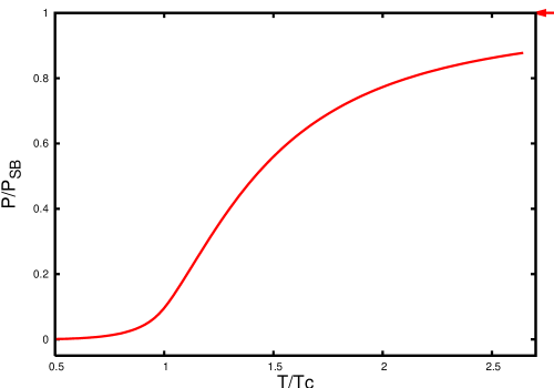
Figure 2: Pressure scaled with Stefan-Boltzmann pressure as function of temperature for $\mu_{0}=0$ from PNJL model. Arrow on the right indicates ideal gas value.

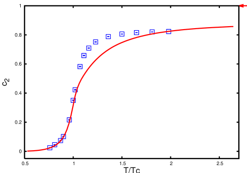
Figure 3: The QNS as a function of $T/T_{c}$. Symbols are Lattice data sixx . Arrow on the right indicates ideal gas value.

We now present the pressure and its derivatives with respect to $\mu_{0}$ at $\mu_{0}=0$. The pressure was fitted to a polynomial in $\mu_{0}$ using the GNU plot program at different values of temperature. The maximum range of $\mu_{0}$ was chosen to be 200 MeV. However near $T_{c}$ the $\chi^{2}$ (which in this case is same as the least square) of the fit varies rapidly with the variation of range of $\mu_{0}$ over which the fit was done, and the actual range was chosen from minima of $\chi^{2}$. The data points were spaced by 0.1 MeV.

In table 1 we present the fitted values of the Taylor coefficients for a few values of temperature to show the dependence of these fitted coefficients on the range of $\mu_{0}$ and number of terms in the polynomial. Due to limitations of numerical accuracy and time, we chose to take a maximum of only upto the eighth order term in $\mu_{0}$. We hope to obtain higher order coefficients in future. The coefficients seem to be quite robust. For each temperature in the table the coefficients in the first case was actually used in the final result.

Fig.2 displays the pressure scaled with that of Stefan-Boltzmann (SB) gas ($P/P_{SB}$) as a function of $T/T_{c}$. Upto $2.5T_{c}$ the pressure grows from almost zero at low temperatures to about 90% of its ideal gas value. This is a bit high when compared to continuum estimates on the Lattice latpr , which is about 80% of $P_{SB}$. A comparison of our results with the PNJL result in Fig.7a of Ref.pnjl2 , shows a near perfect match, though $T_{0}=\rm{270~{}MeV}$ in our measurements compared to their value of $T_{0}=\rm{190~{}MeV}$.

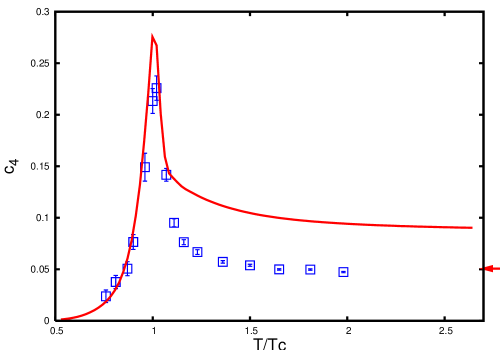
Figure 4: The $c_{4}$ as a function of $T/T_{c}$. The solid line is from PNJL model, Symbols are Lattice data sixx . Arrow on the right indicates ideal gas value.

Next we show the comparison of the coefficients $c_{2}$, $c_{4}$ and $c_{6}$ obtained by us with Lattice data available in Table 3.2 of Ref.sixx . Fig.3 shows the variation of the QNS $c_{2}$ with $T/T_{c}$. This shows an order parameter-like behaviour. Similar behaviour has been observed in another model study sanjay using the Density Dependent Quark Mass (DDQM) model. At higher temperatures the $c_{2}$ reaches almost 85 % of its ideal gas value, consistent with Lattice data.

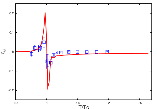
Figure 5: The $c_{6}$ as function of $T/T_{c}$. The solid line is from PNJL model, Symbols are Lattice data sixx .

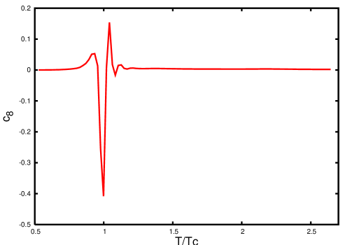
Figure 6: The $c_{8}$ as function of $T/T_{c}$ from PNJL model.

The fourth order derivative $c_{4}$, which can then be thought of as the ”susceptibility” of $c_{2}$ shows a peak at $T=T_{c}$ (Fig.4). Near the transition temperature $T_{c}$, the effective model should work well and we observe that the structure of $c_{4}$ is quite consistent with present day Lattice data eight ; sixx . Just above $T_{c}$ however, there is a significant difference between our results of $c_{4}$ and that of Ref.sixx . While the Lattice values converge to the SB limit, ours is almost double of that value and shows only a weak convergence towards the SB limit. However, our results are consistent with the values of $\chi_{40}$ in Fig.3 in Ref.eight , though it has been argued smalmu4 that these data would come down to the SB limit once a correct continuum limit is taken. Note that in the SB limit both $c_{2}$ and $c_{4}$ have only fermionic contributions. We expect that because the coupling strength is still large in this temperature regime it is unlikely that $c_{4}$ should go to the SB limit within $T<2.5T_{c}$. Moreover, the quark masses used in Ref.sixx is considerably large ($m/T=0.4$) to expect fermionic observables to go to the SB limit. However, it is possible that our overestimation is due to the use of mean field approximation. Recently, in a quasi-particle model soff the Taylor coefficients have been found to match the Lattice data quite accurately. This model uses $c_{2}$ to fix the $T$ and $\mu$ dependence of an effective coupling in the self energy and then predicts the values of the higher order coefficients. In contrast, the PNJL model uses only pure gauge results on the lattice to fix the parameters of the Polyakov loop effective potential and then predicts all the coefficients including $c_{2}$.

The HODs $c_{6}$ and $c_{8}$ are plotted in Fig.5 and Fig.6 respectively. At high temperatures both of these HODs converge to zero. The structure near $T_{c}$ is more interesting. Compared to other models the pattern of the HODs show much better resemblance to the Lattice results. The hadron resonance gas model describes the Lattice data well below $T_{c}$, but fails for $T>T_{c}$ hdrs . The recently proposed shubd scenario of coloured bound states also compares the HODs from Lattice data. However, their comparison at the present state is still not completely satisfactory.

IV.2 $C_{V}$, $v_{s}^{2}$ and ${\cal C}$

We now discuss the results for the other thermodynamic quantities that we have computed. First we consider the specific heat. As shown in Fig.7, $C_{V}$ grows with increasing temperature and reaches a peak at $T_{c}$. Then it decreases sharply for a short range of temperature. Thereafter it shows a broad but shallow bump around $T=\rm{270~{}MeV}$ and then gradually goes to a value little below the ideal gas value. Comparing with the recent lattice data for pure glue theory (Fig.3f, Ref.swa2 ), we see that the difference from the ideal gas value is far less in our case. For comparison, we have also plotted the values of $4\epsilon/T^{4}$, at which the specific heat is expected to coincide for a conformal gas. As is clear from the plot, the values almost coincide at the large temperatures but not as perfectly as in Ref.swa2 .

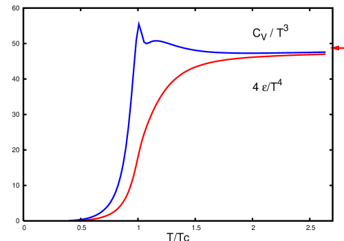
Figure 7: $C_{V}/T^{3}$ and $4\epsilon/T^{4}$ as function of $T/T_{c}$. The arrow on the right shows the ideal gas value.

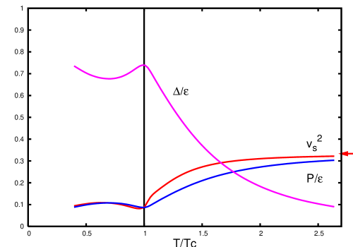
Figure 8: Squared velocity of sound $v_{s}^{2}$ and conformal measure ${\cal C}=\Delta/\epsilon$ as function of $T/T_{c}$. The arrow on the right shows the ideal gas value for $v_{s}^{2}$. For comparison with $v_{s}^{2}$ we also plot the ratio $P/\epsilon$.

Let us now consider the speed of sound and the conformal measure. In view of the possible relation between the two as indicated in (11), we plot both these quantities together in Fig.8. As can be seen from the figure, the two quantities indeed behave in such a correlated manner. We note here that ${\cal C}$ has been computed from the zeroth and first order coefficients of $\Omega(T,\mu_{0}=0)$, whereas the $v_{s}^{2}$ has been measured from the first and second order coefficients. However the relation implied is not exact as can be seen in the figure. The value of $P/\epsilon$ matches with that of $v_{s}^{2}$ for $T<T_{c}$ and also goes close again above $2.5T_{c}$. But in between these two limits the $v_{s}^{2}$ is distinctly greater than $P/\epsilon$. Thus, ${\cal C}$ would go to zero much faster if we replace $P/\epsilon$ by $v_{s}^{2}$ for computing ${\cal C}$.

The $v_{s}^{2}$ is close to its ideal gas value at the temperature of about $2.5T_{c}$. This is close to the results for pure glue theory on the Lattice as reported in Ref.swa2 and also that with 2 flavour Wilson Fermions in Ref.khan , with 2+1 flavours of staggered quarks reported in Ref.szabo , and with improved 2 flavour staggered fermions ($P/\epsilon$ was measured in this case). This possibly refers to an intriguing fact that $v_{s}^{2}$ is dominated by the gluonic degrees of freedom at least for large temperatures. However, near $T_{c}$ the $v_{s}^{2}$ in Ref.swa2 goes to a minimum value above 0.15, whereas we find the minima going close to 0.08, consistent with simulations with dynamical quark in Refs.khan ; szabo , and remarkably close to the softest point $P/\epsilon=0.075$ in Ref.isentropp . This is expected as the scalar $\sigma$ is supposed to be important in chiral dynamics for small quark masses. Even upto temperatures as low as $0.5T_{c}$ the $v_{s}^{2}$ in our case doesn’t go much above 0.1. This is also in contrast with the values reported in Ref.beda , where a confinement model wws has been used. These authors find a value of about $v_{s}^{2}=0.15$ near $T_{c}$ and a value of 0.2 near $0.5T_{c}$. On the other hand $v_{s}^{2}$ (isothermal) measured in Ref.sanjay using the DDQM model, shows a better agreement with our results.

The values for the conformal measure ${\cal C}$ also closely resembles the Lattice data of Ref.swa2 . Near $T_{c}$ there is a slight departure. We find the value ranging from 0.7 to 0.75, whereas those authors find it to vary around 0.6 to 0.7 for pure glue theory. However, note that the dip at temperatures less than $T_{c}$ is prominent in both the cases. At even lower temperatures we find ${\cal C}$ to increase. For a non-relativistic ideal gas, the ratio of $P/\epsilon$ should go to zero, and thus ${\cal C}$ should then go to 1. Thus at lower temperatures such an increase is indeed expected. On the other hand at high temperatures either an ideal gas or a conformal behaviour should be recovered for which ${\cal C}$ should go to zero. Our results in this respect resemble the pure gauge Lattice results very closely.

V Discussions and Summary

We have studied several thermodynamic quantities of recent interest in QCD, in the framework of Polyakov-loop extended NJL (PNJL) model. Inclusion of Polyakov loop in the NJL model covers both the confinement as well as chiral symmetry breaking; the two most important characteristics of low energy QCD. The Polyakov-loop provides with the order parameter for deconfinement transition while the quark condensate acts as the order parameter for chiral transition.

It is well known that the measurement of various fluctuations is of crucial importance to understand the characteristics of transition of confined matter to deconfined state. So, using the PNJL model, we have computed the derivatives of pressure upto eight order. It is expected that the susceptibilities might provide the most direct evidence for the order of QCD phase transition. In fact, a well defined peak in the susceptibility can indicate the cross over transition. On the other hand, a sharp diverging behaviour would indicate the existence of CEP.

In the present paper, we have kept our computation close to $\mu_{0}=0$ axis. The second derivative of pressure $c_{2}$ rises steeply near $T_{c}$ and then saturates near $T=2T_{c}$. This behaviour indicates that near the transition the quark number fluctuations increase with temperature and then gradually saturates at higher temperatures. Such a behaviour is expected both from lattice as well as phenomenological studies. $c_{4}$ has a peak around $T_{c}$, whereas, both $c_{6}$ and $c_{8}$ show rapid variation across $T_{c}$. Considering the inherent differences of model and lattice approaches, our results are in good agreement with the lattice data. There is however a significant difference found in the values of $c_{4}$ in the temperature range starting from a little above $T_{c}$. We speculate this may have occurred due to the neglect of fluctuations around the mean field in our computations; though one should keep in mind the very large masses used in Lattice computations in contrast to the value of $5.5{\rm MeV}$ used in the PNJL model.

We have also calculated the specific heat, speed of sound and the conformal measure. These results again are in close agreement with Lattice data. There seems to be a dominance of gluonic contribution at high temperatures. Near $T_{c}$ however there are small but significant difference in Lattice data with pure QCD and that with dynamical quarks. Our results in this temperature region match well with the latter set.

There are several issues that need to be addressed for a better understanding of the physics of QCD phase transition. NJL model works with constant four point coupling strength, the running coupling being averaged over a limited low energy kinematic domain. To make contact with QCD at high temperatures this coupling should have proper temperature dependence. Moreover, the parameters in the Polyakov-loop part should be tuned to get both the deconfinement and chiral transition within a temperature difference of couple of MeVs at most and also below, say, 200 MeV, as indicated by the Lattice data. Note that similar parameter fitting of the Polyakov-loop in the PNJL model led the authors in Ref.pisarski2 to couple the Polyakov-loop and $SU(3)\times SU(3)$ linear sigma model to study the $K/\pi$ ratio. However, there are more predictions in the present model, the most significant being the possibility of studying the QCD transition at finite baryon densities. Above and all one should also worry about the mean-field approximation involved here. For the Polyakov loop part, it would be worthwhile to explore approches similar to Ref.enrique , where a local Polyakov loop has been coupled to the chiral Lagrangian.

We have not yet studied the system with large chemical potentials. As already noted in Ref.pnjl2 , the PNJL model does have the requisite physics of a first order transition for low temperatures and high chemical potential, a cross-over for $\mu_{0}=0$ and thus a CEP for some $T=T_{E}$ and $\mu_{0}=\mu_{0_{E}}$. The details in this case may be compared to other NJL model studies with high $\mu_{0}$. For example the chiral symmetry broken phase and normal quark matter phase of Ref.njlpd show a similar value of the CEP. Moreover it has been shown in Ref.njltype that with increase of strength of the diquark coupling the CEP moves towards higher temperatures and slightly lower values of $\mu_{0}$. Hence, the inclusion of diquark physics may be important to assess the exact location of the phase boundary as well as the CEP.

A natural extension of our work would be to include the isospin chemical potential and study the behaviour for isospin and electric charge fluctuations. We hope to address some of these issues in future.

References

- (1) F. Carminati et al. , J. Phys. G 30 1517 (2004).
- (2) K. Adcox et al. , Nucl. Phys. A 757 184 (2005).
-
(3)
P. Arnold and C. Zhai, Phys. Rev. D 50 7603 (1994);
ibid Phys. Rev. D 51 1906 (1994);
C. Zhai and B. Kastering, Phys. Rev. D 52 7232 (1995);
E. Braaten and A. Nieto, Phys. Rev. D 53 3421 (1996); ibid Phys. Rev. Lett. 76 1417 (1996). -
(4)
R. D. Pisarski, Phys. Rev. Lett. 63 1129 (1989);
J. Frenkel and J. C. Taylor, Nucl. Phys. B 334 199 (1990). - (5) E. Braaten and R. D. Pisarski, Nucl. Phys. B 337 569 (1990).
- (6) J-P. Blaizot and E. Iancu, Nucl. Phys. B 390 589 (1993); Nucl. Phys. B 417 608 (1994).
- (7) P. F. Kelly, Q. Liu, C. Lucchesi and C. Manuel, Phys. Rev. D 50 4209 (1994).
-
(8)
J. O. Andersen, E. Braaten and M. Strickland,
Phys. Rev. 61 014017 (2000); Phys. Rev. D 61 074016 (2000);
J. O. Andersen and M. Strickland, Phys. Rev. D 66 105001 (2002);
J. O. Andersen, E. Braaten, E. Petitgirard and M. Strickland, Phys. Rev. D 66 085016 (2002);
J. O. Andersen, E. Petitgirard and M. Strickland, Phys. Rev. 70 045001 (2004). - (9) A. Peshier, Phys. Rev. 63 105004 (2001).
-
(10)
J-P. Blaizot, E. Iancu and A. Rebhan, Phys. Rev. Lett. 83 2906
(1999);
Phys. Lett. B 470 181 (1999); Phys. Rev. D 63 065003 (2001). - (11) J-P. Blaizot, E. Iancu and A. Rebhan, Phys. Lett. B 523 143 (2001); Eur. Phys. C 27 433 (2003).
-
(12)
P. Chakraborty, M. G. Mustafa and M. H. Thoma,
Eur. Phys. C 23 591 (2002);
Phys. Rev. D 68 085012 (2003); Phys. Rev. D 67 114004 (2003). - (13) F. Karsch, M. G. Mustafa and M. H. Thoma, Phys. Lett. B 497 249 (2001).
- (14) W. M. Albercico, A. Beraudo and A. Molinary, Nucl. Phys. A 750 359 (2005).
-
(15)
P. Ginsparg, Nucl. Phys. B 170 388 (1980);
T. Appelquist and R. D. Pisarski, Phys. Rev. D 23 2305 (1981);
E. Braaten and A. Nieto, Phys. Rev. D 53 3421 (1996);
K. Kajantie, M. Laine, R. Rummukainen and M. Shaposhnikov, Nucl. Phys. B 458 90 (1996). -
(16)
K. Kajantie et al. , Phys. Rev. Lett. 79 3130 (1997);
Nucl. Phys. B 503 357 (1997);
M. Laine and O. Philipsen, Nucl. Phys. B 523 267 (1998); Phys. Lett. B 459 259 (1999). - (17) K. Kajantie, M. Laine, K. Rummukainen and Y. Schröeder, Phys. Rev. Lett. 86 10 (2001).
- (18) A. Vuorinen, Phys. Rev. D 68 054017 (2003); hep-ph/0402242.
- (19) E. Laermann and O. Philipsen, Ann. Rev. Nucl. Part. Sci. 53 163 (2003).
- (20) Z. Fodor and S. Katz, Phys. Lett. B 534 87 (2002).
-
(21)
M.P. Lombardo and M. d’Elia,
Phys. Rev. D 67 014505 (2003);
Ph. de Forcrand and O. Philipsen, Nucl. Phys. B 673 170 (2003). -
(22)
S. Gottlieb et al. , Phys. Rev. Lett. 59 2247 (1987);
S. Choe et al. , Phys. Rev. D 65 054501 (2002). - (23) C. R. Allton et al. , Phys. Rev. D 68 014507 (2003).
-
(24)
R. V. Gavai and S. Gupta, Phys. Rev. D 68 034506 (2003);
R. V. Gavai and S. Gupta, Nucl. Phys. Proc. Suppl. B 129 524 (2004);
S. Gupta and R. Ray Phys. Rev. D 70 114015 (2004). - (25) R. V. Gavai and S. Gupta, Phys. Rev. D 72 054006 (2005).
- (26) C. R. Allton et al. , Phys. Rev. D 71 054508 (2005).
-
(27)
L. D. McLerran and B. Svetitsky,
Phys. Rev. D 24 450 (1981);
B. Svetitsky and L. G. Yaffe, Nucl. Phys. B 210 423 (1982);
B. Svetitsky, Phys. Rept. 132, 1 (1986). -
(28)
R. D. Pisarski, Phys. Rev. D 62 111501 (2000);
”Marseille 2000, Strong and electroweak matter” pg. 107-117 (hep-ph/0101168). - (29) E. Megias, E. Ruiz Arriola, L.L. Salcedo, Phys. Rev. D 69 116003 (2004).
- (30) D. Diakonov and M. Oswald, Phys. Rev. D 70, 105016 (2004).
-
(31)
A. Dumitru and R. D. Pisarski,
Phys. Lett. B 504 282 (2001);
Phys. Rev. D 66 096003 (2002); Nucl. Phys. A 698 444 (2002). - (32) O. Scavenius, A. Dumitru and J. T. Lenaghan, Phys. Rev. C 66 034903 (2002).
- (33) E. Megias, E. R. Arriola, L. L. Salcedo, J. H. E. P. 0601 073 (2006).
-
(34)
B. Layek, A. P. Mishra and A. M. Srivastava,
Phys. Rev. D 71 074015 (2005);
B. Layek, A. P. Mishra, A. M. Srivastava and V. K. Tiwari, hep-ph/0512367. -
(35)
M. Alford, K. Rajagopal, and F. Wilczek,
Phys. Lett. B 422 247 (1998);
R. Rapp, T. Schäfer, E. V. Shuryak, and M. Velkovsky, Phys. Rev. Lett. 81 53 (1998). - (36) J. Berges and K. Rajagopal, Nucl. Phys. B 538 215 (1999).
- (37) M. A. Halasz et al. , Phys. Rev. D 58 096007 (1998).
-
(38)
S. P. Klevansky, Rev. Mod. Phys. 64 649 (1992);
A. Barducci, R. Casalbuoni, G. Pettini, and R. Gatto, Phys. Rev. D 49 426 (1994). - (39) M. A. Stephanov, Phys. Rev. Lett. 76 4472 (1996); Nucl. Phys. B (Proc. Suppl.) 53 469 (1997).
- (40) M. Stephanov, K. Rajagopal, E. Shuryak, Phys. Rev. Lett. 81 4816 (1998).
- (41) H. Abuki and T. Kunihiro, Nucl. Phys. A 768 118 (2006).
- (42) Z. Fodor and S. D. Katz, J. H. E. P. 0404 050 (2004).
- (43) Z. Fodor and S. D. Katz, J. H. E. P. 0203 014 (2002).
- (44) P. N. Meisinger and M. C. Ogilvie, Phys. Lett. B 379 163 (1996); Nucl. Phys. B (Proc. Suppl.) 47 519 (1996).
- (45) E. Megias, E. R. Arriola, L. L. Salcedo, hep-ph/0412308.
-
(46)
M. Asakawa, U. Heinz and B. Müller,
Phys. Rev. Lett. 85 2072 (2000);
S. Jeon and V. Koch, Phys. Rev. Lett. 85 2076 (2000). -
(47)
H. Appelshauser and H. Sako, for the CERES
Collaboration, Nucl. Phys. A 752 394 (2005);
J. T. Mitchell and the PHENIX Collaboration, J. Phys. Conf. Ser. 27 88 (2005). - (48) L. Stodolsky, Phys. Rev. Lett. 75 1044 (1995).
- (49) R. Korus et al. , Phys. Rev. C 64 054908 (2001).
- (50) J. Ollitrault, Phys. Rev. D 46 229 (1992).
- (51) H. Sorge, Phys. Rev. Lett. 82 2048 (1999).
-
(52)
P. F. Kolb et al. , Phys. Lett. B 459 667 (1999);
P. F. Kolb et al. , Nucl. Phys. A 661 349 (1999). -
(53)
D. Teaney et al. , Phys. Rev. Lett. 86 4783 (2001);
D. Teaney et al. , nucl-th/0110037 - (54) B. Mohanty and J. Alam, Phys. Rev. C 68 064903 (2003).
- (55) R. V. Gavai, S. Gupta and S. Mukherjee, Phys. Rev. D 71 074013 (2005).
- (56) R. V. Gavai, S. Gupta and S. Mukherjee, hep-lat/0506015.
- (57) G. Policastro, D. T. Son and A. Starinets, Phys. Rev. Lett. 87 081601 (2001).
- (58) D. Teaney, Phys. Rev. C 68 034913 (2003).
-
(59)
A. Nakamura and S. Sakai, Phys. Rev. Lett. 94 072305 (2005);
S. Gupta, Phys. Lett. B 597 57 (2004). - (60) Y. Nambu and G. Jona-Lasinio, Phys. Rev. 122 345 (1961); Phys. Rev. 124 246 (1961).
-
(61)
U. Vogl and W. Weise, Prog. Part. Nucl. Phys. 27 195 (1991);
S. P. Klevansky, Rev. Mod. Phys. 64 649 (1992);
T. Hatsuda and T. Kunihiro, Phys. Rept. 247 221 (1991);
M. Buballa, Phys. Rept. 407 205 (2005). - (62) K. Fukushima, Phys. Lett. , B 591 277 (2004).
- (63) C. Ratti, M.A. Thaler and W. Weise, Phys. Rev. D 73 014019 (2006).
- (64) S. Digal, E. Laermann, H. Satz, Eur. Phys. C 18 583 (2001).
- (65) P. N. Messinger, M. C. Ogilvie and T. R. Miller, Phys. Lett. B 585 149 (2004).
-
(66)
G. Boyd et al. , Nucl. Phys. B 469 419 (1996);
Y. Iwasaki et al. Phys. Rev. D 56 151 (1997). -
(67)
B. Beinlich et al. , Eur. Phys. C 6 133 (1999);
M. Okamoto et al. , Phys. Rev. D 60 094510 (1999). -
(68)
P. de Forcrand et al. , Nucl. Phys. B 577 263 (2000);
Y. Namekawa et al. , Phys. Rev. D 64 074507 (2001). -
(69)
S. Gupta, Phys. Rev. D 64 034507 (2001);
F. Karsch, E. Laermann and A. Peikert, Nucl. Phys. B 605 579 (2001);
A. Ali Khan et al. , Phys. Rev. D 63 034502 (2001). - (70) F. Karsch, E. Laermann and A. Peikert, Phys. Lett. B 478 447 (2000).
- (71) S. K. Ghosh, T. K. Mukherjee and S. Raha, nucl-th/0509086 (to appear in Mod. Phys. Lett. A ).
- (72) M. Bluhm, B. Kämpfer and G. Soff, Phys. Lett. B 620 131 (2005).
- (73) S. Ejiri, F. Karsch and K. Redlich, Phys. Lett. B 633 275 (2006).
- (74) J. Liao and E. V. Shuryak Phys. Rev. D 73 014509 (2006).
- (75) A. Ali Khan et al. Phys. Rev. D 64 074510 (2001).
- (76) Y. Aoki, Z. Fodor, S. D. Katz and K. K. Szabo, J. H. E. P. 0601 089 (2006).
- (77) S. Ejiri, F. Karsch, E. Laermann and C. Schmidt, hep-lat/0512040.
- (78) R. A. Schneider and W. Weise, Phys. Rev. C 64 055201 (2001).
- (79) S. B. Ruster, et.al., Phys. Rev. D 72 034004 (2005).