Deep inelastic beauty production at HERA
in the $k_{T}$-factorization approach

D.V. Skobeltsyn Institute of Nuclear Physics,
M.V. Lomonosov Moscow State University,
119992 Moscow, Russia

Abstract

We calculate the cross section of beauty production in $ep$ deep inelastic scattering at HERA collider in the framework of the $k_{T}$-factorization approach. The unintegrated gluon distributions in a proton are obtained from the full CCFM, from unified BFKL-DGLAP evolution equations as well as from the Kimber-Martin-Ryskin prescription. We investigate different production rates and study the $b$-quark contribution to the inclusive proton structure function $F_{2}(x,Q^{2})$ at small $x$ and at moderate and high values of $Q^{2}$. Our theoretical results are compared with the recent experimental data taken by the H1 and ZEUS collaborations. We demonstrate the importance of leading $\ln 1/x$ contributions in description of the HERA data.

1 Introduction

The beauty production at high energies is a subject of intensive study from both theoretical and experimental points of view [1–9]. First measurements [1] of the $b$-quark cross sections at HERA were significantly higher than the QCD predictions calculated at next-to-leading order (NLO) approximation. Similar observations were made in hadron-hadron collisions at Tevatron [2] and also in photon-photon interactions at LEP2 [3]. In last case, the theoretical NLO QCD predictions are more than three standard deviations below the experimental data. At Tevatron, recent analisys indicates that the overall description of the data can be improved [10] by adopting the non-perturbative fragmentation function of the $b$-quark into the $B$-meson: an appropriate treatment of the $b$-quark fragmentation properties considerably reduces the disagreement between measured beauty cross section and the results of corresponding NLO QCD calculations. Also latest measurements [4, 5, 9] of the beauty photoproduction at HERA are in a reasonable agreement with the NLO QCD predictions or somewhat higher. Some disagreement is observed mainly at small decay muon and/or associated jet transverse momenta [4, 5, 9]. But the large excess of the first measurements over NLO QCD, reported by the H1 collaboration [1], is not confirmed.

Recently there have been become available experimental data [6–9] on the $b$-quark production in deep inelastic scattering at HERA which taken by the H1 and ZEUS collaborations. The first measurements [6, 7] of the beauty contribution to the inclusive proton structure function $F_{2}(x,Q^{2})$ have been presented for small values of the Bjorken scaling variable $x$, namely $2\cdot 10^{-4}<x<5\cdot 10^{-3}$, and for moderate and high values of the photon virtuality $Q^{2}$, namely $12<Q^{2}<700$ GeV². Also process $e+p\to e^{\prime}+b+\bar{b}+X\to e^{\prime}+{\rm jet}+\mu+X^{\prime}$ has been measured [8, 9] in the small $x$ region with at least one jet and a decay muon in the final state and still was not described in the framework of QCD theory. Such processes are dominated by the photon-gluon fusion subprocess $\gamma^{*}+g\to b+\bar{b}$ and therefore sensitive to the gluon density in a proton $xg(x,\mu^{2})$. It was claimed [8, 9] that the NLO QCD calculations have some difficulties in description of the recent HERA data. The predictions at low values of $Q^{2}$, Bjorken $x$, muon transverse momentum and high values of jet transverse energy and muon pseudo-rapidity is about two standard deviation below the data.

In the present paper to analyze the recent H1 and ZEUS data [6–9] we use the so-called $k_{T}$-factorization [11, 12] (or semi-hard [13, 14]) approach of QCD which has been applied earlier, in particular, in description of the charm and beauty production at HERA [15–21], Tevatron [22–28] and LEP2 [19, 29, 30] colliders. The $k_{T}$-factorization approach is based on the Balitsky-Fadin-Kuraev-Lipatov (BFKL) [31] or Ciafaloni-Catani-Fiorani-Marchesini (CCFM) [32] gluon evolution which are valid at small $x$ since here large logarithmic terms proportional to $\ln 1/x$ are summed up to all orders of perturbation theory (in the leading logarithmic approximation). It is in contrast with the popular Dokshitzer-Gribov-Lipatov-Altarelli-Parizi (DGLAP) [33] strategy where only large logarithmic terms proportional to $\ln\mu^{2}$ are taken into account. The basic dynamical quantity of the $k_{T}$-factorization approach is the so-called unintegrated (${\mathbf{k}}_{T}$-dependent) gluon distribution ${\cal A}(x,{\mathbf{k}}_{T}^{2},\mu^{2})$ which determines the probability to find a gluon carrying the longitudinal momentum fraction $x$ and the transverse momentum ${\mathbf{k}}_{T}$ at the probing scale $\mu^{2}$. The unintegrated gluon distribution can be obtained from the analytical or numerical solution of the BFKL or CCFM evolution equations. Similar to DGLAP, to calculate the cross sections of any physical process the unintegrated gluon density ${\cal A}(x,{\mathbf{k}}_{T}^{2},\mu^{2})$ has to be convoluted [11–14] with the relevant partonic cross section $\hat{\sigma}$. But as the virtualities of the propagating gluons are no longer ordered, the partonic cross section has to be taken off mass shell (${\mathbf{k}}_{T}$-dependent). It is in clear contrast with the DGLAP scheme (so-called collinear factorization). Since gluons in initial state are not on-shell and are characterized by virtual masses (proportional to their transverse momentum), it also assumes a modification of their polarization density matrix [13, 14]. In particular, the polarization vector of a gluon is no longer purely transversal, but acquires an admixture of longitudinal and time-like components. Other important properties of the $k_{T}$-factorization formalism are the additional contribution to the cross sections due to the integration over the ${\mathbf{k}}_{T}^{2}$ region above $\mu^{2}$ and the broadening of the transverse momentum distributions due to extra transverse momentum of the colliding partons.

As it was noted already, some applications of the $k_{T}$-factorization approach supplemented with the BFKL and CCFM evolution to the heavy (charm and beauty) quark production at high energies are widely discussed in the literature [15–30] (see also review [34, 35]). It was shown [24–28] that the beauty cross section at Tevatron can be consistently described in the framework of this approach. However, a substantial discrepancy between theory and experiment is still found [19, 29, 30] for the $b$-quark production in $\gamma\gamma$ collisions at LEP2, not being cured by the $k_{T}$-factorization. At HERA, the inclusive beauty photoproduction has been investigated [16, 17, 19, 21, 25]. In [17, 19, 25] comparisons with the first H1 measurements [1] have been done. In [17, 25] the Monte-Carlo generator Cascade [36] has been used to predict the cross section of the $b$-quark and dijet associated photoproduction. However, calculations [17, 19, 25] deal with the total cross sections only. In our previous paper [21] the total and differential cross sections of beauty photoproduction (both inclusive and associated with hadronic jets) have been considered and comparisons with the recent H1 and ZEUS measurements [1, 4, 5, 9] have been made. It was demonstrated [21] that the $k_{T}$-factorization approach supplemented with the CCFM or BFKL-DGLAP evolved unintegrated gluon distributions [28, 37] reproduces well the numerous HERA data [1, 4, 5, 9].

In the present paper we will study the beauty production in $ep$ deep inelastic scattering at HERA. We investigate a number of different production rates (in particular, the transverse momentum and pseudo-rapidity distributions of muons which originate from the semi-leptonic decays of $b$-quarks). Our study is based on leading-order (LO) off-mass shell matrix elements for the photon-gluon fusion subprocess $e+g^{*}\to e^{\prime}+b+\bar{b}$. Particularly we discuss the photoproduction limit ($Q^{2}\to 0$) of our derivation. Also we investigate the beauty contribution to the inclusive proton structure function $F_{2}(x,Q^{2})$. In the numerical analysis we test the unintegrated gluon distributions which were obtained [28, 37] from the full CCFM, unified BFKL-DGLAP evolution equations and from the conventional parton densities (using the Kimber-Martin-Ryskin prescription [38]). We attempted a systematic comparison of model predictions with the recent experimental data [6–9] taken by the H1 and ZEUS collaborations. One of purposes of this paper is to investigate the specific $k_{T}$-factorization effects in the $b$-quark leptoproduction at HERA.

The outline of our paper is following. In Section 2 we recall the basic formulas of the $k_{T}$-factorization approach with a brief review of calculation steps. In Section 3 we present the numerical results of our calculations and a discussion. Finally, in Section 4, we give some conclusions. The compact analytic expressions for the off-mass shell matrix elements of the photon-gluon fusion subprocess $e+g^{*}\to e^{\prime}+b+\bar{b}$ are given in Appendix. These formulas may be useful for the subsequent applications.

2 Calculation details

In this section we present our analytic results for the cross section of $e+p\to e^{\prime}+b+\bar{b}+X$ in DIS. We work at leading-order $k_{T}$-factorization approach of QCD. We start by defining the kinematics.

2.1 Kinematics

We denote the four-momenta of the incoming electron and proton and the outgoing electron, beauty quark and anti-quark by $p_{e}$, $p_{p}$, $p_{e}^{\prime}$, $p_{b}$ and $p_{\bar{b}}$, respectively. The off-shell gluon and virtual photon have four-momenta $k$ and $q$, and it is customary to define

$$k^{2}=k_{T}^{2}=-{\mathbf{k}}_{T}^{2}<0,\quad q^{2}=(p_{e}-p_{e}^{\prime})^{2}=q_{T}^{2}=-Q^{2}<0,$$

where $k_{T}$ and $q_{T}$ are the transverse four-momenta of the corresponding particles. Choosing a suitable coordinate system in the $ep$ center-of-mass frame, we have

$$p_{e}={\sqrt{s}}/2\,(1,0,0,-1),\quad p_{p}={\sqrt{s}}/2\,(1,0,0,1),$$

where $\sqrt{s}$ is the total energy of the process under consideration and we neglect the masses of the incoming electron and proton. The standard deep inelastic variables $x$ and $y$ are defined as usual:

$$x={Q^{2}\over 2(p_{p}\cdot q)},\quad y={(p_{p}\cdot q)\over(p_{e}\cdot p_{p})}\simeq{Q^{2}\over xs}.$$

The variable $y$ measures the relative electron energy loss in the proton rest frame. From the conservation law we can easily obtain the following condition:

$$\quad{\mathbf{k}}_{T}+{\mathbf{q}}_{T}={\mathbf{p}}_{b\,T}+{\mathbf{p}}_{\bar{b}\,T}.$$

2.2 Cross section for deep inelastic beauty production

According to the $k_{T}$-factorization theorem, the cross section of deep inelastic beauty production $e+p\to e^{\prime}+b+\bar{b}+X$ can be written as a convolution

$$\sigma(e+p\to e^{\prime}+b+\bar{b}+X)=\int{dx\over x}{\cal A}(x,{\mathbf{k}}_{T}^{2},\mu^{2})d{\mathbf{k}}_{T}^{2}{d\phi\over 2\pi}d\hat{\sigma}(e+g^{*}\to e^{\prime}+b+\bar{b}),$$

where ${\cal A}(x,{\mathbf{k}}_{T}^{2},\mu^{2})$ is the unintegrated gluon distribution in a proton, $\hat{\sigma}(e+g^{*}\to e^{\prime}+b+\bar{b})$ is the cross section of partonic subprocess and $\phi$ is the azimuthal angle of initial virtual gluon. Decomposing the cross section $\hat{\sigma}(e+g^{*}\to e^{\prime}+b+\bar{b})$ into a leptonic and a hadronic part, we can write it as

$$d\sigma(e+g^{*}\to e^{\prime}+b+\bar{b})={1\over 64xs}{e^{2}\over Q^{4}}L^{\mu\nu}H_{\mu\nu}\,d\Phi^{(3)}(p_{e}+k,p_{e}^{\prime},p_{b},p_{\bar{b}}),$$

where $e$ is the electron charge magnitude and $L^{\mu\nu}$ and $H^{\mu\nu}$ are the leptonic and hadronic tensors. In general case the Lorentz-invariant element $d\Phi^{(n)}(p,p_{1},\ldots,p_{n})$ of $n$-body phase space is given by

$$d\Phi^{(n)}(p,p_{1},\ldots,p_{n})=(2\pi^{4})\,\delta^{(4)}\left(p-\sum_{i=1}^{n}p_{i}\right)\prod_{i=1}^{n}{d^{3}p_{i}\over(2\pi)^{3}2p_{i}^{0}}.$$

Integrating over the azimuthal angle of the outgoing electron, we can simplify (6) to become

$$d\sigma(e+g^{*}\to e^{\prime}+b+\bar{b})={\alpha\over 2\pi}{1\over 64xs}L^{\mu\nu}H_{\mu\nu}{dy\over y}{dQ^{2}\over Q^{2}}d\Phi^{(2)}(q+k,p_{b},p_{\bar{b}}),$$

where $\alpha=e^{2}/(4\pi)$ is Sommerfeld’s fine structure constant. For the leptonic tensor $L^{\mu\nu}$ we use the following expression [39]:

$$L^{\mu\nu}={1+(1-y)^{2}\over y}\epsilon^{\mu\nu}_{T}-{4(1-y)\over y}\epsilon^{\mu\nu}_{L},$$

where

$$\epsilon^{\mu\nu}_{T}=-g^{\mu\nu}+{q^{\mu}k^{\nu}+q^{\nu}k^{\mu}\over(q\cdot k)}-{q^{2}\over(q\cdot k)^{2}}k^{\mu}k^{\nu},\atop{\displaystyle\epsilon^{\mu\nu}_{L}={1\over q^{2}}\left(q^{\mu}-{q^{2}\over(q\cdot k)}k^{\mu}\right)\left(q^{\nu}-{q^{2}\over(q\cdot k)}k^{\nu}\right)}.$$

The $\epsilon^{\mu\nu}_{T}$ and $\epsilon^{\mu\nu}_{L}$ refer to transverse and longitudinal virtual photon polarization, as indicated by their subscripts. It is easily to see that $q_{\mu}\epsilon^{\mu\nu}_{T}=q_{\mu}\epsilon^{\mu\nu}_{L}=0$, $\epsilon^{\mu}_{\mu\,T}=-2$ and $\epsilon^{\mu}_{\mu\,L}=-1$. Furthermore,

$$\epsilon^{\mu\nu}=\epsilon^{\mu\nu}_{T}+\epsilon^{\mu\nu}_{L}=-g^{\mu\nu}+{q^{\mu}q^{\nu}\over q^{2}},$$

i.e. $\epsilon^{\mu\nu}$ is the polarization tensor of an unpolarized spin-one boson having mass $q^{2}$. From (5) — (10) one can obtain the following formula for the cross section of deep inelastic beauty production in the $k_{T}$-factorization approach:

$$\sigma(e+p\to e^{\prime}+b+\bar{b}+X)=\int{1\over 256\pi^{3}(xys)^{2}}{\cal A}(x,{\mathbf{k}}_{T}^{2},\mu^{2})\times\atop\displaystyle\times\left[{(1+(1-y)^{2})\over Q^{2}}T({\mathbf{k}}_{T}^{2},Q^{2})-4(1-y)L({\mathbf{k}}_{T}^{2},Q^{2})\right]d{\mathbf{p}}_{b\,T}^{2}d{\mathbf{k}}_{T}^{2}dQ^{2}dy_{b}dy_{\bar{b}}{d\phi\over 2\pi}{d\phi_{b}\over 2\pi}{d\phi_{\bar{b}}\over 2\pi},$$

where $y_{b}$, $y_{\bar{b}}$ and $\phi_{b}$ and $\phi_{\bar{b}}$ are the rapidities and azimuthal angles of the produced beauty quark and anti-quark, respectively. The evaluation of functions $T({\mathbf{k}}_{T}^{2},Q^{2})$ and $L({\mathbf{k}}_{T}^{2},Q^{2})$ has been done analytically using the Mathematica 5 program. The compact expressions for these functions are listed in Appendix. It is important that the functions $T({\mathbf{k}}_{T}^{2},Q^{2})$ and $L({\mathbf{k}}_{T}^{2},Q^{2})$ depend on the virtual gluon non-zero transverse momentum ${\mathbf{k}}_{T}^{2}$. Note that if we average (12) over ${\mathbf{k}}_{T}$ and take the limit ${\mathbf{k}}_{T}^{2}\to 0$, then we obtain well-known formula corresponding to the usual LO QCD calculations.

It is interesting to study the photoproduction limit of (12) by taking the limit $Q^{2}\to 0$. This provides us with a powerful check for our formulas by relating them to well-known results. So, the cross section of the partonic process $\gamma+g^{*}\to b+\bar{b}$ reads

$$d\sigma(\gamma+g^{*}\to b+\bar{b})={1\over 64\hat{s}}(-g^{\mu\nu})H_{\mu\nu}\biggm{|}_{Q^{2}=0}d\Phi^{(2)}(q+k,p_{b},p_{\bar{b}}),$$

where $\hat{s}=(q+k)^{2}$. Comparing (8) and (13), one can obtain the well-known relation

$$\lim_{Q^{2}\to 0}Q^{2}{d\sigma(e+g^{*}\to e^{\prime}+b+\bar{b})\over dydQ^{2}}={\alpha\over 2\pi}{1+(1-y)^{2}\over y}\sigma(\gamma+g^{*}\to b+\bar{b}).$$

The contribution of $b$-quarks to the deep inelastic proton structure function $F_{2}(x,Q^{2})$ can be calculated according to convolution (5) also. The relevant coefficient function is described by the quark box diagram and has been presented in our previous paper [40].

The multidimensional integration in (12) has been performed by means of the Monte Carlo technique, using the routine Vegas [41]. The full C$++$ code is available from the authors on request.

3 Numerical results

We now are in a position to present our numerical results. First we describe our theoretical input and the kinematical conditions.

3.1 Theoretical uncertainties

There are several parameters which determined the normalization factor of the cross section (12): the beauty mass $m_{b}$, the factorization and normalisation scales $\mu_{F}$ and $\mu_{R}$ and the unintegrated gluon distributions in a proton ${\cal A}(x,{\mathbf{k}}_{T}^{2},\mu^{2})$.

Concerning the unintegrated gluon densities in a proton, in the numerical calculations we used five different sets of them, namely the J2003 (set 1 — 3) [28], KMS [37] and KMR [38]. All these distributions are widely discussed in the literature (see, for example, review [34, 35] for more information). Here we only shortly discuss their characteristic properties. First, three sets of the J2003 gluon density have been obtained [28] from the numerical solution of the full CCFM equation. The input parameters were fitted to describe the proton structure function $F_{2}(x,Q^{2})$. Note that the J2003 set 1 and J2003 set 3 densities contain only singular terms in the CCFM splitting function $P_{gg}(z)$. The J2003 set 2 gluon density takes into account the additional non-singlular terms. These distributions have been applied in the analysis of the forward jet production at HERA and charm and bottom production at Tevatron [28] (in the framework of Monte-Carlo generator Cascade [36]) and have been used also in our calculations [20, 21].

Another set (the KMS) [37] was obtained from a unified BFKL-DGLAP description of $F_{2}(x,Q^{2})$ data and includes the so-called consistency constraint [42]. The consistency constraint introduces a large correction to the LO BFKL equation. It was argued [43] that about 70% of the full NLO corrections to the BFKL exponent $\Delta$ are effectively included in this constraint. The KMS gluon density is successful in description of the beauty hadroproduction at Tevatron [24, 26] and photoproduction at HERA [21].

The last, fifth unintegrated gluon distribution ${\cal A}(x,{\mathbf{k}}_{T}^{2},\mu^{2})$ used here (the so-called KMR distribution) is the one which was originally proposed in [38]. The KMR approach is the formalism to construct unintegrated gluon distribution from the known conventional parton (quark and gluon) densities. It accounts for the angular-ordering (which comes from the coherence effects in gluon emission) as well as the main part of the collinear higher-order QCD corrections. The key observation here is that the $\mu$ dependence of the unintegrated parton distribution enters at the last step of the evolution, and therefore single scale evolution equations (DGLAP or unified BFKL-DGLAP) can be used up to this step. Also it was shown [38] that the unintegrated distributions obtained via unified BFKL-DGLAP evolution are rather similar to those based on the pure DGLAP equations. It is because the imposition of the angular ordering constraint is more important [38] than including the BFKL effects. Based on this point, in our further calculations we use much more simpler DGLAP equation up to the last evolution step. Note that the KMR parton densities in a proton were used, in particular, to describe the prompt photon photoproduction at HERA [45] and prompt photon hadroproduction Tevatron [46, 47].

Also the significant theoretical uncertainties in our results connect with the choice of the factorization and renormalization scales. First of them is related to the evolution of the gluon distributions, the other is responsible for the strong coupling constant $\alpha_{s}(\mu^{2}_{R})$. The optimal values of these scales are such that the contribution of higher orders in the perturbative expansion is minimal. As it often done for beauty production, we choose the renormalization and factorization scales to be equal: $\mu_{R}=\mu_{F}=\mu=\sqrt{m_{b}^{2}+\langle{\mathbf{p}}_{T}^{2}\rangle}$, where $\langle{\mathbf{p}}_{T}^{2}\rangle$ is set to the average ${\mathbf{p}}_{T}^{2}$ of the beauty quark and antiquark. But in the case of the KMS gluon distribution we used special choice $\mu^{2}={\mathbf{k}}_{T}^{2}$, as it was originally proposed in [37]. Note that in the present paper we concentrate mostly on the non-collinear gluon evolution in the proton and do not study the scale dependence of our results. To completeness, we take the $b$-quark mass $m_{b}=4.75$ GeV and use LO formula for the coupling constant $\alpha_{s}(\mu^{2})$ with $n_{f}=4$ active quark flavours at $\Lambda_{\rm QCD}=200$ MeV, such that $\alpha_{s}(M_{Z}^{2})=0.1232$.

3.2 Associated beauty and jet production

The recent experimental data [8, 9] for the associated beauty and hadronic jet leptoproduction at HERA comes from both the H1 and ZEUS collaborations. The total and differential cross sections as a function of the photon virtuality $Q^{2}$, Bjorken scaling variable $x$, muon transverse momentum $p_{T}^{\mu}$ and pseudo-rapidity $\eta^{\mu}$ and jet transverse momentum $p_{T}^{\rm jet}$ have been determined. The ZEUS data [8] refer to the kinematical region defined by $Q^{2}>2$ GeV² with at least one hadron-level jet (in the Breit frame) with $p_{T}^{\rm jet\,Breit}>6$ GeV and $-2<\eta^{\rm jet}<2.5$ and with muon which fulfill the following conditions: $-0.9<\eta^{\mu}<1.3$ and $p_{T}^{\mu}>2$ GeV or $-1.6<\eta^{\mu}<-0.9$ and $p^{\mu}>2$ GeV. The fraction $y$ of the electron energy transferred to the photon is restricted to the range $0.05<y<0.7$. Note that the Breit frame is defined by the usual condition ${\mathbf{q}}+2x{\mathbf{p}_{p}}=0$. In this frame, a space-like photon and proton collide head-on and any final-state particle with a high transverse momentum is produced by a hard QCD interaction. The more recent H1 data [9] refer to the kinematical region defined by $2<Q^{2}<100$ GeV², $0.1<y<0.7$, $p_{T}^{\mu}>2.5$ GeV, $-0.75<\eta^{\mu}<1.15$, $p_{T}^{\rm jet\,Breit}>6$ GeV and $|\eta^{\rm jet}|<2.5$. To produce muons from $b$-quarks in our theoretical calculations, we first convert $b$-quarks into $B$-hadrons using the Peterson fragmentation function [48] and then simulate their semileptonic decay according to the standard electroweak theory. Of course, the muon transverse momenta spectra are sensitive to the fragmentation functions. However, this dependence is expected to be small as compared with the uncertainties coming from the unintegrated gluon densities in a proton. Our default set of the fragmentation parameter is $\epsilon_{b}=0.0035$.

The basic photon-gluon fusion subprocess $\gamma^{*}+g^{*}\to b+\bar{b}$ give rise to two high-energy $b$-quarks, which can further evolve into hadron jets. In our calculations we assumed that the produced quarks (with their known kinematical parameters) are taken to play the role of the final jets. These two quarks are accompanied by a number of gluons radiated in the course of the gluon evolution. As it has been noted in [15], on the average the gluon transverse momentum decreases from the hard interaction block towards the proton. We assume that the gluon emitted in the last evolution step and having the four-momenta $k^{\prime}$ compensates the whole transverse momentum of the gluon participating in the hard subprocess, i.e. ${\mathbf{k}^{\prime}}_{T}\simeq-{\mathbf{k}}_{T}$. All the other emitted gluons are collected together in the proton remnant, which is assumed to carry only a negligible transverse momentum compared to ${\mathbf{k}^{\prime}}_{T}$. This gluon gives rise to a final hadron jet with $p_{T}^{\rm jet}=|{\mathbf{k}^{\prime}}_{T}|$ in addition to the jet produced in the hard subprocess. From these three hadron jets we choose the one carrying the largest transverse momentum (in the Breit frame), and then compute the beauty and associated jet production rates.

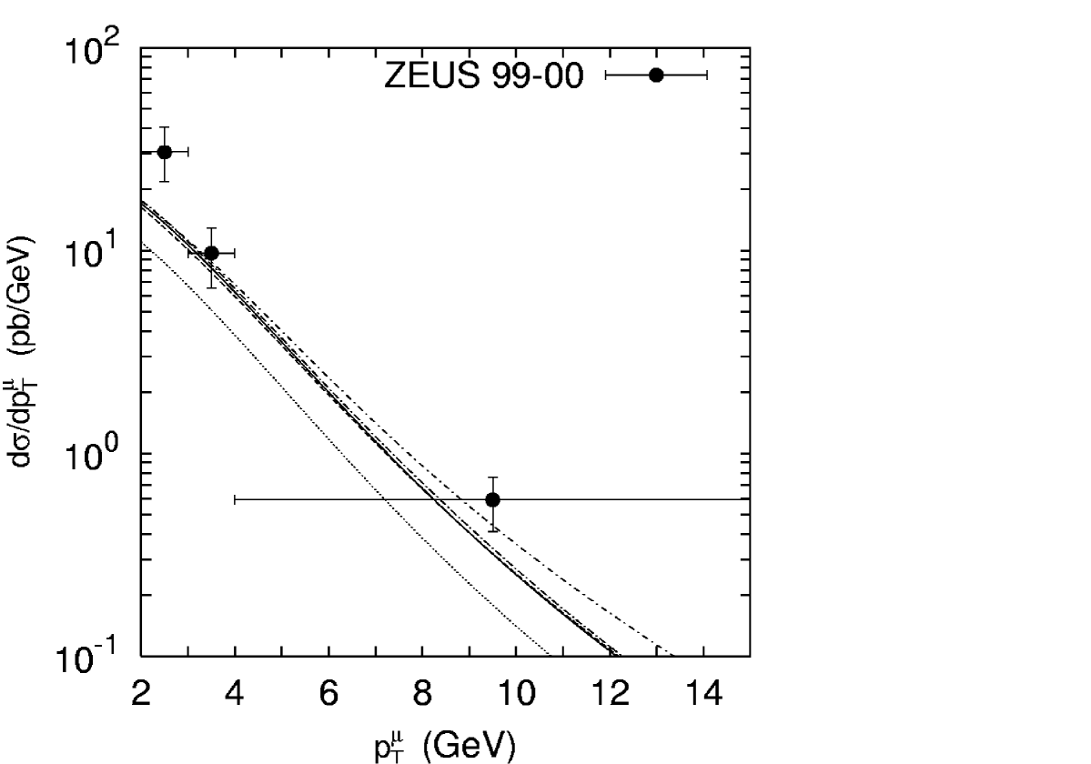
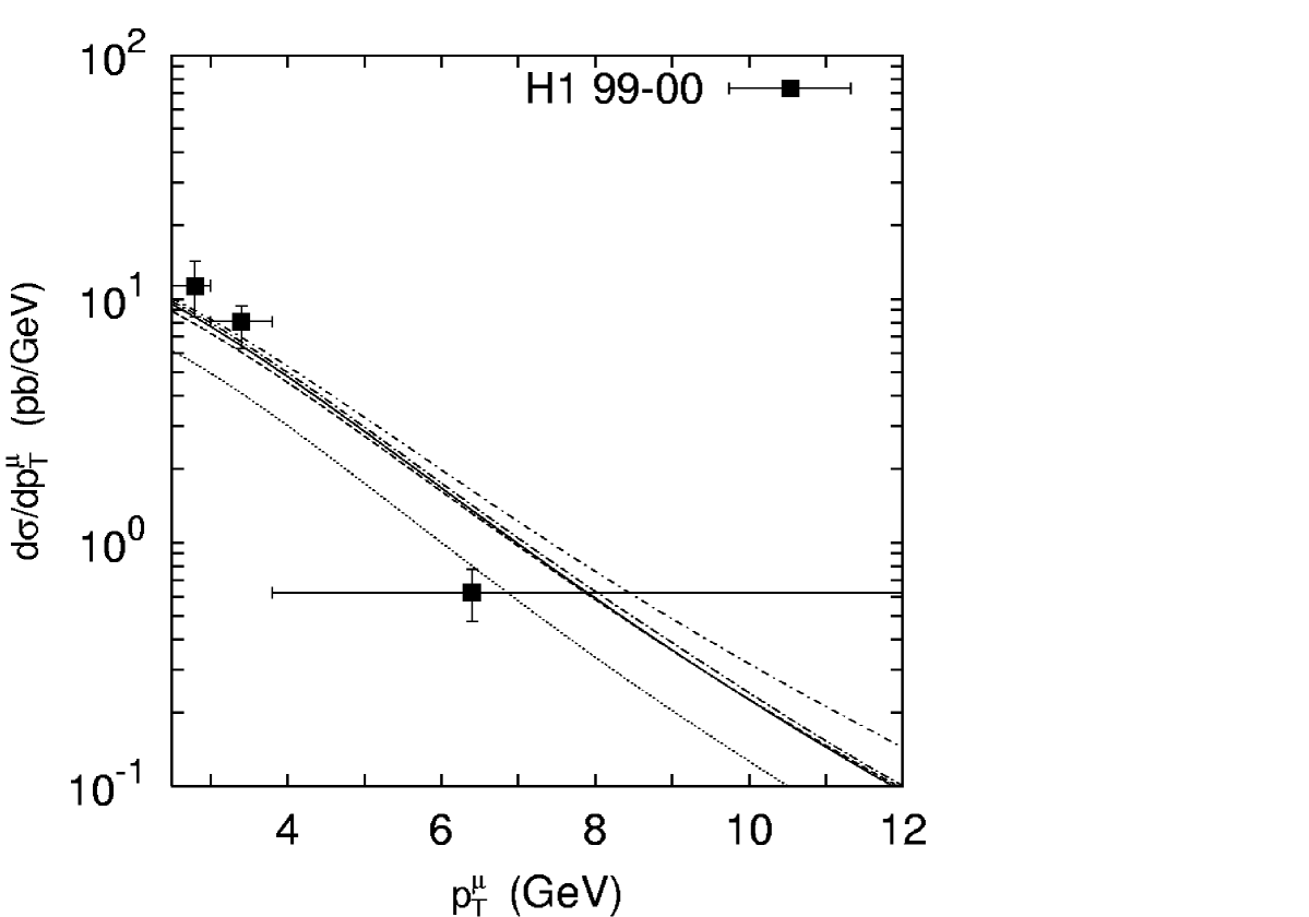
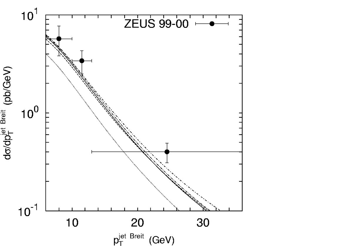
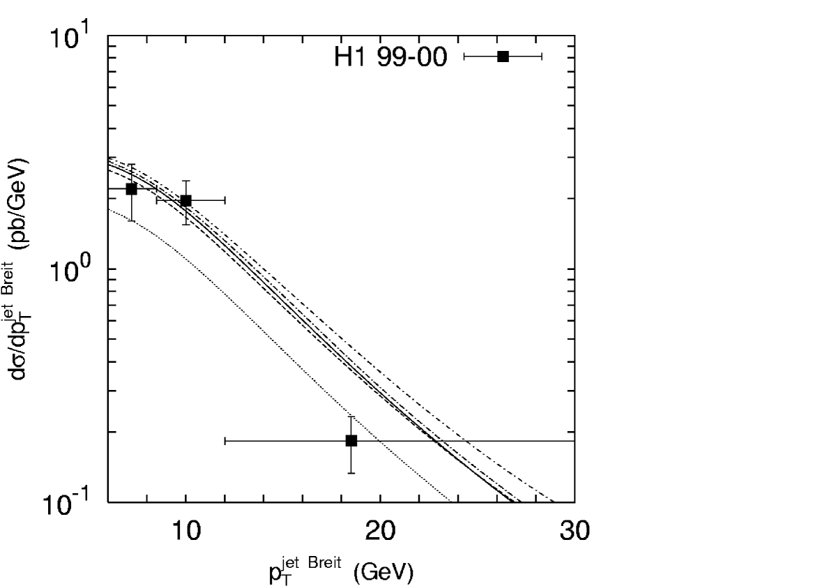
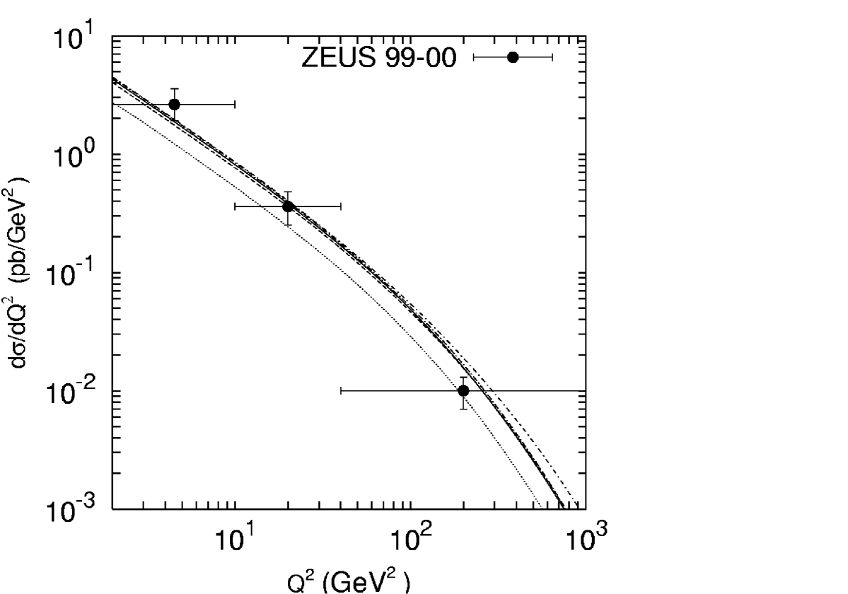
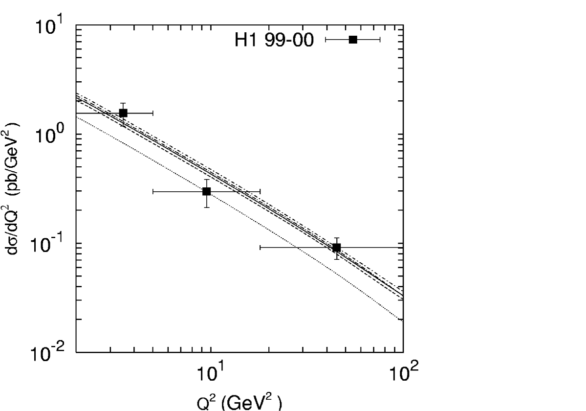
The results of our calculations are shown in Figs. 1 — 10 in comparison to the H1 and ZEUS experimental data [8, 9] fo the $b$-quark and associated jet production. Solid, dashed, dash-dotted, dotted and short dash-dotted curves correspond to the predictions obtained with the J2003 set 1 — 3, KMR and KMS unintegrated gluon densities, respectively. One can see that the overall agreement between our results (calculated using the J2003 and KMS gluon densities) and experimental data [8, 9] is a rather good. However, the measured cross section as a function of the muon transverse momentum $p_{T}^{\mu}$ shows a slightly steeper behaviour than the theoretical predictions: the results of our calculations tends to underestimate the data at low $p_{T}^{\mu}$ (see Figs. 1 and 2). But in general these predictions still agree with the H1 and ZEUS data within the experimental uncertainties. Note also that the measured differential cross sections $d\sigma/d\eta^{\mu}$ in Figs. 3 and 4 exhibit a rise towards the forward muon pseudo-rapidity region, which is not reproduced [8, 9] by the collinear NLO calculations. At the same time the shape and the normalization of $\eta^{\mu}$ distributions are well described by our calculations. The collinear NLO QCD underestimate also the data at low $Q^{2}$ and low $x$ values: it was claimed that in these kinematical regions the data are about two standard deviation higher [8, 9].

As it was already mentioned above, the absolute normalization of the predicted cross sections in the framework of $k_{T}$-factorization approach is depends on the unintegrated gluon distribution used. From Figs. 1 — 10 one can see that all three sets of the J2003 gluon density as well as the KMS one give rise to results which are rather close to each other. So, the difference in normalization between the KMS and J2003 predictions is rather small, is about 15% only. The similar effect we have found [21] in the case of beauty photoproduction. However, it is in the contrast with the $D^{*}$ meson and dijet associated photoproduction, which has been investigated in our previous paper [20]. It was demonstrated [20] a relative large enhancement of the cross sections calculated using the KMS gluon density. The possible explanation of this fact is that the large $b$-quark mass (which provide a hard scale) makes predictions of the perturbation theory of QCD more applicable. Note also that the KMS gluon density provides a more hard transverse momentum distribution of the final muon (or jet) as compared with other unintegrated densities under consideration. Similar effect we have observed [21] in the case of beauty photoproduction.

Concerning the KMR predictions, one can see that this unintegrated gluon distribution gives results which lie below the data and which are very similar to the collinear NLO QCD. Such observation coincides with the ones [20, 21]. This fact confirms the assumption which was made in [45] that the KMR formalism results in some underestimation of the predicted cross sections. Such underestimation can be explained by the fact that leading logarithmic terms proportional to $\ln 1/x$ are not included into the KMR approach.

Source	$\sigma(e+p\to e^{\prime}+{\rm jet}+\mu+X)$ [pb]
ZEUS measurement [8]	$40.9\pm 5.7~{}{\rm(stat.)}^{+6.0}_{-4.4}~{}{\rm(syst.)}$
NLO QCD (hvqdis [50])	$20.6^{+3.1}_{-2.2}$
Rapgap [48]	14.0
Cascade [36]	28.0
J2003 set 1	35.27
J2003 set 2	33.47
J2003 set 3	36.75
KMR	22.11
KMS	38.52

Table 1: The total cross section of beauty and associated jet leptoproduction obtained in the kinematic range $Q^{2}>2$ GeV², $0.05<y<0.7$, $p_{T}^{\rm jet\,Breit}>6$ GeV, $-2<\eta^{\rm jet}<2.5$ and $p_{T}^{\mu}>2$ GeV, $-0.9<\eta^{\mu}<1.3$ or $p^{\mu}>2$ GeV, $-1.6<\eta^{\mu}<-0.9$.

Now we turn to the total cross section of $b$-quark and associated jet leptoproduction. In Table 1 and 2 we compare our theoretical results with the H1 and ZEUS data [8, 9] obtained in relevant kinematical regions (defined above). The predictions of Monte-Carlo generators Rapgap [49], Cascade [36] as well as NLO QCD calculations (hvqdis program) [50] are also shown for comparison. One can see that the collinear NLO QCD predictions is about 2.5 standard deviation lower than the ZEUS data and is about 1.8 standard deviation lower then the H1 data. At the same time, our predictions obtained using the J2003 and KMS gluon densities are significantly higher and agree well with the both H1 and ZEUS data within the experimental uncertainties. The KMR unintegrated gluon distribution again gives the results which are below the data and which are very close to NLO QCD ones. Note that the Monte-Carlo generators Rapgap and Cascade also predict a lower cross section than that measured in the data.

In general, we can conclude that the cross sections of deep inelastic beauty and associated jet production calculated in the $k_{T}$-factorization formalism (supplemented with the CCFM or unified BFKL-DGLAP evolution) are larger by $30-40$% than ones calculated at NLO level of collinear QCD. This enhancement comes, in particular, from the non-zero transverse momentum of the incoming off-shell gluons and from taken into account the leading $\ln 1/x$ terms. Our results for the total and differential cross sections are in a better agreement (both in normalization and shape) with the H1 and ZEUS data than the NLO QCD predictions.

Source	$\sigma(e+p\to e^{\prime}+{\rm jet}+\mu+X)$ [pb]
H1 measurement [9]	$16.3\pm 2.0~{}{\rm(stat.)}\pm 2.3~{}{\rm(syst.)}$
NLO QCD (hvqdis [50])	$9.0^{+2.6}_{-1.6}$
Rapgap [49]	6.3
Cascade [36]	9.8
J2003 set 1	19.96
J2003 set 2	18.98
J2003 set 3	20.80
KMR	12.45
KMS	22.61

Table 2: The total cross section of beauty and associated jet leptoproduction obtained in the kinematic range $2<Q^{2}<100$ GeV², $0.1<y<0.7$, $p_{T}^{\mu}>2.5$ GeV, $-0.75<\eta^{\mu}<1.15$, $p_{T}^{\rm jet\,Breit}>6$ GeV and $|\eta^{\rm jet}|<2.5$.

3.3 Beauty contribution to the proton SF $F_{2}(x,Q^{2})$

Now we will concentrate on the $b$-quark contribution to the inclusive proton structure function $F_{2}(x,Q^{2})$. We will use the master formulas which were obtained in our previous paper [40]. As it was mentioned above, the first experimental data [6, 7] on the structure function $F_{2}^{b}(x,Q^{2})$ comes from the H1 collaboration. These data refer to the kinematical region defined by $2\cdot 10^{-4}<x<5\cdot 10^{-3}$ and $12<Q^{2}<650$ GeV².

Note that we change now the default set of parameters which we have used in the previous section. So, we set the renormalization and factorization scales $\mu_{R}$ and $\mu_{F}$ to be equal to photon virtuality $Q^{2}$, as it was done earlier in analysis [51] of the charm contribution to the structure function $F_{2}(x,Q^{2})$ in the framework of $k_{T}$-factorization QCD approach. The similar choice have been used also in the analysis of longitudinal structure function $F_{L}(x,Q^{2})$ [52]. Of course, in the case of the KMS gluon distribution we set $\mu^{2}_{R}=\mu^{2}_{F}={\mathbf{k}}_{T}^{2}$, as it was originally proposed in [37]. Other parameters have not been changed.

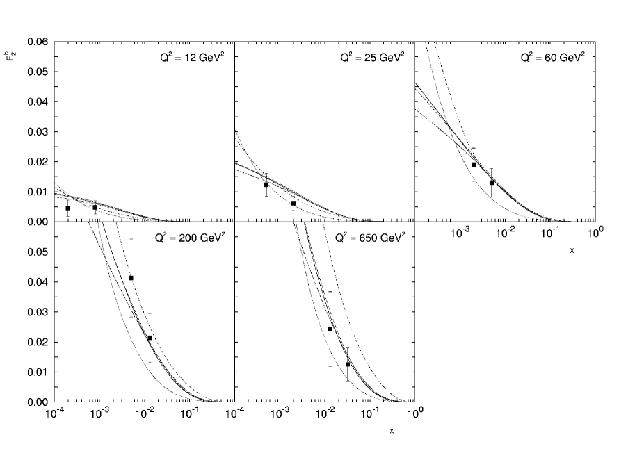
In Fig. 11 we show the structure function $F_{2}^{b}(x,Q^{2})$ as a function of $x$ for different values of $Q^{2}$ in comparison to the recent H1 data [6, 7]. One can see that the J2003 distributions reproduce well the experimental data for all values of $Q^{2}$. The KMS gluon density demonstrates a perfect agreement with the data at moderate $Q^{2}$ but slightly overestimate them at $Q^{2}=650$ GeV². It is interesting to note that the KMR density does not contradict the experimental data, too. However, this distribution predicts a more rapid rise of the calculated function $F_{2}^{b}(x,Q^{2})$ with decreasing of $x$ (in comparison to the J2003 and KMS densities). We can conclude that in the small $x$ region ($x<10^{-2}$) the shape of function $F_{2}^{b}(x,Q^{2})$ predicted by the unintegrated gluon distributions under consideration is very different. In particular, the differences observed between the curves are due to the different behaviour of the corresponding unintegrated gluon distributions as a function of $x$ and ${\mathbf{k}}_{T}^{2}$ [45]. This fact shows the importance of a detail understanding of the non-collinear parton evolution in a proton and the necessarity of better experimental constraints as well as further theoretical studies in this field.

4 Conclusions

We have calculated the deep inelastic beauty and associated jet production in electron-proton collisions at HERA in the $k_{T}$-factorization QCD approach. The total and several differential cross section (as a function of the photon virtuality $Q^{2}$, Bjorken scaling variable $x$, decay muon transverse momentum $p_{T}^{\mu}$ and pseudo-rapidity $\eta^{\mu}$ and hadronic jet transverse momentum $p_{T}^{\rm jet}$) have been studied. Additionally we have investigated the $b$-quark contribution to the inclusive proton structure function $F_{2}(x,Q^{2})$ at small $x$ and at moderate and high $Q^{2}$. In numerical analysis we have used the unintegrated gluon densities which are obtained from the full CCFM (J2003 set 1 — 3), from unified BFKL-DGLAP evolution equations (KMS) as well as from the Kimber-Martin-Ryskin prescription. Our investigations were based on the LO off-mass shell matrix elements for photon-gluon fusion subprocesses.

We have shown that the $k_{T}$-factorization approach supplemented with the CCFM or BFKL-DGLAP evolved unintegrated gluon distributions (the J2003 or KMS densities) reproduces well the numerous HERA data on beauty and associated jet production. At the same time we have obtained that the Kimber-Martin-Ryskin formalism results in some underestimation of the cross sections. This shows the importance of a detail understanding of the non-collinear parton evolution process.

5 Acknowledgements

The authors are very grateful to S.P. Baranov and A.V. Kotikov for their encouraging interest and very helpful discussions. This research was supported in part by the FASI of Russian Federation (grant NS-1685.2003.2).

6 Appendix

Here we present the compact analytic expressions for the functions $T({\mathbf{k}}_{T}^{2},Q^{2})$ and $L({\mathbf{k}}_{T}^{2},Q^{2})$ which appear in (12). In the following, $\hat{s}$, $\hat{t}$ and $\hat{u}$ are usual Mandelstam variables for corresponding $\gamma^{*}+g^{*}\to b+\bar{b}$ subprocesses ($\hat{s}+\hat{t}+\hat{u}=2m^{2}-Q^{2}-{\mathbf{k}}_{T}^{2}$) and $m$ and $e_{b}$ is the mass and fractional electric charge of $b$-quark. The exact expressions for the functions $T({\mathbf{k}}_{T}^{2},Q^{2})$ and $L({\mathbf{k}}_{T}^{2},Q^{2})$ can be presented as

$$T({\mathbf{k}}_{T}^{2},Q^{2})=(4\pi)^{3}\alpha^{2}\alpha_{s}(\mu^{2})e_{b}^{2}\,{F_{T}(\hat{s},\hat{t},\hat{u},{\mathbf{k}}_{T}^{2},Q^{2})\over 8(\hat{t}-m^{2})^{2}(\hat{u}-m^{2})^{2}(\hat{s}+Q^{2}+{\mathbf{k}}_{T}^{2})^{4}},$$

$$L({\mathbf{k}}_{T}^{2},Q^{2})=(4\pi)^{3}\alpha^{2}\alpha_{s}(\mu^{2})e_{b}^{2}\,{F_{L}(\hat{s},\hat{t},\hat{u},{\mathbf{k}}_{T}^{2},Q^{2})\over 8(\hat{t}-m^{2})^{2}(\hat{u}-m^{2})^{2}(\hat{s}+Q^{2}+{\mathbf{k}}_{T}^{2})^{4}},$$

where

$$F_{T}(\hat{s},\hat{t},\hat{u},{\mathbf{k}}_{T}^{2},Q^{2})=-8(4{\mathbf{k}}_{T}^{8}Q^{4}(\hat{t}-\hat{u})^{2}+2{\mathbf{k}}_{T}^{6}Q^{2}(-8m^{8}+{\hat{t}}^{4}+4Q^{4}(\hat{t}-\hat{u})^{2}-$$

$$4{\hat{t}}^{3}\hat{u}-2{\hat{t}}^{2}{\hat{u}}^{2}-4\hat{t}{\hat{u}}^{3}+{\hat{u}}^{4}+16m^{6}(\hat{t}+\hat{u})+4Q^{2}(\hat{t}-\hat{u})^{2}(\hat{t}+\hat{u})-8m^{4}({\hat{t}}^{2}+$$

$$4\hat{t}\hat{u}+{\hat{u}}^{2})-8m^{2}(Q^{2}(\hat{t}-\hat{u})^{2}-2\hat{t}\hat{u}(\hat{t}+\hat{u})))+$$

$$(\hat{s}+Q^{2}+{\mathbf{k}}_{T}^{2})^{2}(24m^{12}+8m^{10}(Q^{2}-3(\hat{t}+\hat{u}))-2m^{8}(2Q^{4}+3{\hat{t}}^{2}+$$

$$22\hat{t}\hat{u}+3{\hat{u}}^{2}+10Q^{2}(\hat{t}+\hat{u}))-\hat{t}\hat{u}({\hat{t}}^{2}+{\hat{u}}^{2})(2Q^{4}+2Q^{2}(\hat{t}+\hat{u})+(\hat{t}+\hat{u})^{2})+$$

$$m^{2}({\hat{t}}^{5}+13{\hat{t}}^{4}\hat{u}+26{\hat{t}}^{3}{\hat{u}}^{2}+26{\hat{t}}^{2}{\hat{u}}^{3}+13\hat{t}{\hat{u}}^{4}+{\hat{u}}^{5}+2Q^{4}(\hat{t}+\hat{u})^{3}+$$

$$4Q^{2}\hat{t}\hat{u}(3{\hat{t}}^{2}+4\hat{t}\hat{u}+3{\hat{u}}^{2}))+4m^{6}(2Q^{4}(\hat{t}+\hat{u})+Q^{2}(3{\hat{t}}^{2}+14\hat{t}\hat{u}+3{\hat{u}}^{2})+$$

$$4({\hat{t}}^{3}+6{\hat{t}}^{2}\hat{u}+6\hat{t}{\hat{u}}^{2}+{\hat{u}}^{3}))-m^{4}(7{\hat{t}}^{4}+56{\hat{t}}^{3}\hat{u}+90{\hat{t}}^{2}{\hat{u}}^{2}+56\hat{t}{\hat{u}}^{3}+7{\hat{u}}^{4}+$$

$$6Q^{4}(\hat{t}+\hat{u})^{2}+2Q^{2}({\hat{t}}^{3}+19{\hat{t}}^{2}\hat{u}+19\hat{t}{\hat{u}}^{2}+{\hat{u}}^{3})))-2{\mathbf{k}}_{T}^{4}(8m^{12}-2Q^{8}(\hat{t}-\hat{u})^{2}-$$

$$4Q^{6}(\hat{t}-\hat{u})^{2}(\hat{t}+\hat{u})+\hat{t}\hat{u}(\hat{t}+\hat{u})^{2}({\hat{t}}^{2}+{\hat{u}}^{2})-4Q^{4}({\hat{t}}^{4}-2{\hat{t}}^{3}\hat{u}-2{\hat{t}}^{2}{\hat{u}}^{2}-2\hat{t}{\hat{u}}^{3}+{\hat{u}}^{4})-$$

$$Q^{2}({\hat{t}}^{5}-5{\hat{t}}^{4}\hat{u}-4{\hat{t}}^{3}{\hat{u}}^{2}-4{\hat{t}}^{2}{\hat{u}}^{3}-5\hat{t}{\hat{u}}^{4}+{\hat{u}}^{5})+8m^{10}(2Q^{2}-3(\hat{t}+\hat{u}))+2m^{8}(8Q^{4}-$$

$$12Q^{2}(\hat{t}+\hat{u})+15(\hat{t}+\hat{u})^{2})-4m^{6}(8Q^{4}(\hat{t}+\hat{u})+5(\hat{t}+\hat{u})^{3}+$$

$$Q^{2}(-5{\hat{t}}^{2}+2\hat{t}\hat{u}-5{\hat{u}}^{2}))+m^{4}(7{\hat{t}}^{4}+32{\hat{t}}^{3}\hat{u}+42{\hat{t}}^{2}{\hat{u}}^{2}+32\hat{t}{\hat{u}}^{3}+7{\hat{u}}^{4}+$$

$$8Q^{4}({\hat{t}}^{2}+10\hat{t}\hat{u}+{\hat{u}}^{2})-2Q^{2}(5{\hat{t}}^{3}-13{\hat{t}}^{2}\hat{u}-13\hat{t}{\hat{u}}^{2}+5{\hat{u}}^{3}))+m^{2}(-{\hat{t}}^{5}+$$

$$8Q^{6}(\hat{t}-\hat{u})^{2}-9{\hat{t}}^{4}\hat{u}-14{\hat{t}}^{3}{\hat{u}}^{2}-14{\hat{t}}^{2}{\hat{u}}^{3}-9\hat{t}{\hat{u}}^{4}-{\hat{u}}^{5}+8Q^{4}({\hat{t}}^{3}-5{\hat{t}}^{2}\hat{u}-$$

$$5\hat{t}{\hat{u}}^{2}+{\hat{u}}^{3})+4Q^{2}({\hat{t}}^{4}-5{\hat{t}}^{3}\hat{u}-4{\hat{t}}^{2}{\hat{u}}^{2}-5\hat{t}{\hat{u}}^{3}+{\hat{u}}^{4})))+{\mathbf{k}}_{T}^{2}(32m^{14}-$$

$$112m^{12}(\hat{t}+\hat{u})-8m^{10}(4Q^{4}-17{\hat{t}}^{2}-50\hat{t}\hat{u}-17{\hat{u}}^{2})-$$

$$2\hat{t}\hat{u}(\hat{t}+\hat{u})^{3}({\hat{t}}^{2}+{\hat{u}}^{2})+Q^{2}({\hat{t}}^{2}-{\hat{u}}^{2})^{2}({\hat{t}}^{2}-4\hat{t}\hat{u}+{\hat{u}}^{2})+$$

$$2Q^{6}({\hat{t}}^{4}-4{\hat{t}}^{3}\hat{u}-2{\hat{t}}^{2}{\hat{u}}^{2}-4\hat{t}{\hat{u}}^{3}+{\hat{u}}^{4})+2Q^{4}({\hat{t}}^{5}-5{\hat{t}}^{4}\hat{u}-$$

$$4{\hat{t}}^{3}{\hat{u}}^{2}-4{\hat{t}}^{2}{\hat{u}}^{3}-5\hat{t}{\hat{u}}^{4}+{\hat{u}}^{5})-4m^{8}(4Q^{6}+19{\hat{t}}^{3}-$$

$$14Q^{2}(\hat{t}-\hat{u})^{2}+121{\hat{t}}^{2}\hat{u}+121\hat{t}{\hat{u}}^{2}+19{\hat{u}}^{3}-12Q^{4}(\hat{t}+\hat{u}))+4m^{6}(5{\hat{t}}^{4}+$$

$$72{\hat{t}}^{3}\hat{u}+126{\hat{t}}^{2}{\hat{u}}^{2}+72\hat{t}{\hat{u}}^{3}+5{\hat{u}}^{4}+8Q^{6}(\hat{t}+\hat{u})-20Q^{2}(\hat{t}-\hat{u})^{2}(\hat{t}+\hat{u})-$$

$$2Q^{4}(5{\hat{t}}^{2}-2\hat{t}\hat{u}+5{\hat{u}}^{2}))-2m^{4}({\hat{t}}^{5}+49{\hat{t}}^{4}\hat{u}+118{\hat{t}}^{3}{\hat{u}}^{2}+118{\hat{t}}^{2}{\hat{u}}^{3}+49\hat{t}{\hat{u}}^{4}+$$

$${\hat{u}}^{5}+8Q^{6}({\hat{t}}^{2}+4\hat{t}\hat{u}+{\hat{u}}^{2})-3Q^{2}(\hat{t}-\hat{u})^{2}(7{\hat{t}}^{2}+10\hat{t}\hat{u}+7{\hat{u}}^{2})-$$

$$2Q^{4}(5{\hat{t}}^{3}-13{\hat{t}}^{2}\hat{u}-13\hat{t}{\hat{u}}^{2}+5{\hat{u}}^{3}))+2m^{2}(16Q^{6}\hat{t}\hat{u}(\hat{t}+\hat{u})+$$

$$2\hat{t}\hat{u}(\hat{t}+\hat{u})^{2}(5{\hat{t}}^{2}+4\hat{t}\hat{u}+5{\hat{u}}^{2})-Q^{2}(\hat{t}-\hat{u})^{2}(5{\hat{t}}^{3}+3{\hat{t}}^{2}\hat{u}+$$

$$3\hat{t}{\hat{u}}^{2}+5{\hat{u}}^{3})-4Q^{4}({\hat{t}}^{4}-5{\hat{t}}^{3}\hat{u}-4{\hat{t}}^{2}{\hat{u}}^{2}-5\hat{t}{\hat{u}}^{3}+{\hat{u}}^{4})))),$$

$$F_{L}(\hat{s},\hat{t},\hat{u},{\mathbf{k}}_{T}^{2},Q^{2})=16(2{\mathbf{k}}_{T}^{8}Q^{2}(\hat{t}-\hat{u})^{2}+{\mathbf{k}}_{T}^{6}(\hat{t}-\hat{u})^{2}(2m^{4}+4Q^{4}+{\hat{t}}^{2}+{\hat{u}}^{2}+$$

$$4Q^{2}(\hat{t}+\hat{u})-2m^{2}(4Q^{2}+\hat{t}+\hat{u}))+2(m^{2}-\hat{t})(m^{2}-\hat{u})(\hat{s}+Q^{2}+{\mathbf{k}}_{T}^{2})^{2}(2m^{6}+$$

$$m^{4}(Q^{2}-\hat{t}-\hat{u})+\hat{t}\hat{u}(Q^{2}+\hat{t}+\hat{u})-m^{2}(2\hat{t}\hat{u}+Q^{2}(\hat{t}+\hat{u})))+{\mathbf{k}}_{T}^{4}(-8m^{8}Q^{2}+$$

$$2Q^{6}(\hat{t}-\hat{u})^{2}+4Q^{4}(\hat{t}-\hat{u})^{2}(\hat{t}+\hat{u})+(\hat{t}-\hat{u})^{4}(\hat{t}+\hat{u})+$$

$$Q^{2}(3{\hat{t}}^{4}-6{\hat{t}}^{3}\hat{u}-2{\hat{t}}^{2}{\hat{u}}^{2}-6\hat{t}{\hat{u}}^{3}+3{\hat{u}}^{4})+8m^{6}(-(\hat{t}-\hat{u})^{2}+2Q^{2}(\hat{t}+\hat{u}))-$$

$$2m^{4}(-4(\hat{t}-\hat{u})^{2}(\hat{t}+\hat{u})+Q^{2}({\hat{t}}^{2}+22\hat{t}\hat{u}+{\hat{u}}^{2}))-2m^{2}(4Q^{4}(\hat{t}-\hat{u})^{2}+$$

$$2(\hat{t}-\hat{u})^{2}({\hat{t}}^{2}+{\hat{u}}^{2})+Q^{2}(3{\hat{t}}^{3}-11{\hat{t}}^{2}\hat{u}-11\hat{t}{\hat{u}}^{2}+3{\hat{u}}^{3})))+2{\mathbf{k}}_{T}^{2}(4m^{12}-$$

$$4m^{10}(2Q^{2}+3(\hat{t}+\hat{u}))+m^{8}(-4Q^{4}+17{\hat{t}}^{2}+26\hat{t}\hat{u}+17{\hat{u}}^{2}+12Q^{2}(\hat{t}+\hat{u}))+$$

$$2m^{6}(4Q^{4}(\hat{t}+\hat{u})-5(\hat{t}+\hat{u})^{3}-Q^{2}({\hat{t}}^{2}+6\hat{t}\hat{u}+{\hat{u}}^{2}))-\hat{t}\hat{u}(2Q^{4}({\hat{t}}^{2}+{\hat{u}}^{2})+$$

$$(\hat{t}+\hat{u})^{2}({\hat{t}}^{2}-3\hat{t}\hat{u}+{\hat{u}}^{2})+Q^{2}(3{\hat{t}}^{3}+{\hat{t}}^{2}\hat{u}+\hat{t}{\hat{u}}^{2}+3{\hat{u}}^{3}))+2m^{2}(Q^{4}(\hat{t}+\hat{u})^{3}+$$

$$\hat{t}\hat{u}({\hat{t}}^{3}-7{\hat{t}}^{2}\hat{u}-7\hat{t}{\hat{u}}^{2}+{\hat{u}}^{3})+Q^{2}({\hat{t}}^{4}+5{\hat{t}}^{3}\hat{u}+5\hat{t}{\hat{u}}^{3}+{\hat{u}}^{4}))-m^{4}(6Q^{4}(\hat{t}+\hat{u})^{2}+$$

$$Q^{2}(5{\hat{t}}^{3}+3{\hat{t}}^{2}\hat{u}+3\hat{t}{\hat{u}}^{2}+5{\hat{u}}^{3})-2({\hat{t}}^{4}+5{\hat{t}}^{3}\hat{u}+18{\hat{t}}^{2}{\hat{u}}^{2}+5\hat{t}{\hat{u}}^{3}+{\hat{u}}^{4})))).$$

Figure 1: The muon transverse momentum distribution $d\sigma/dp_{T}^{\mu}$ of the deep inelastic beauty production at HERA in the kinematic range $Q^{2}>2$ GeV², $0.05<y<0.7$, $p_{T}^{\rm jet\,Breit}>6$ GeV, $-2<\eta^{\rm jet}<2.5$ and $p_{T}^{\mu}>2$ GeV, $-0.9<\eta^{\mu}<1.3$ or $p^{\mu}>2$ GeV, $-1.6<\eta^{\mu}<-0.9$. The solid, dashed, dash-dotted, dotted and short dash-dotted curves correspond to the predictions obtained with the J2003 set 1 — 3, KMR and KMS unintegrated gluon densities, respectively. The experimental data are from ZEUS [8].

Figure 2: The muon transverse momentum distribution $d\sigma/dp_{T}^{\mu}$ of the deep inelastic beauty production at HERA in the kinematic range $2<Q^{2}<100$ GeV², $0.1<y<0.7$, $p_{T}^{\rm jet\,Breit}>6$ GeV, $|\eta^{\rm jet}|<2$, $p_{T}^{\mu}>2$ GeV and $-0.75<\eta^{\mu}<1.15$. Notations of all curves are the same as in Fig. 1. The experimental data are from H1 [9].

Figure 3: The muon pseudo-rapidity distribution $d\sigma/d\eta^{\mu}$ of the deep inelastic beauty production at HERA in the kinematic range $Q^{2}>2$ GeV², $0.05<y<0.7$, $p_{T}^{\rm jet\,Breit}>6$ GeV, $-2<\eta^{\rm jet}<2.5$ and $p_{T}^{\mu}>2$ GeV, $-0.9<\eta^{\mu}<1.3$ or $p^{\mu}>2$ GeV, $-1.6<\eta^{\mu}<-0.9$. Notations of all curves are the same as in Fig. 1. The experimental data are from ZEUS [8].

Figure 4: The muon pseudo-rapidity distribution $d\sigma/d\eta^{\mu}$ of the deep inelastic beauty production at HERA in the kinematic range $2<Q^{2}<100$ GeV², $0.1<y<0.7$, $p_{T}^{\rm jet\,Breit}>6$ GeV, $|\eta^{\rm jet}|<2$, $p_{T}^{\mu}>2$ GeV and $-0.75<\eta^{\mu}<1.15$. Notations of all curves are the same as in Fig. 1. The experimental data are from H1 [9].

Figure 5: The jet transverse momentum distribution $d\sigma/dp_{T}^{\rm jet\,Breit}$ of the deep inelastic beauty production at HERA in the kinematic range $Q^{2}>2$ GeV², $0.05<y<0.7$, $p_{T}^{\rm jet\,Breit}>6$ GeV, $-2<\eta^{\rm jet}<2.5$ and $p_{T}^{\mu}>2$ GeV, $-0.9<\eta^{\mu}<1.3$ or $p^{\mu}>2$ GeV, $-1.6<\eta^{\mu}<-0.9$. Notations of all curves are the same as in Fig. 1. The experimental data are from ZEUS [8].

Figure 6: The jet transverse momentum distribution $d\sigma/dp_{T}^{\rm jet\,Breit}$ of the deep inelastic beauty production at HERA in the kinematic range $2<Q^{2}<100$ GeV², $0.1<y<0.7$, $p_{T}^{\rm jet\,Breit}>6$ GeV, $|\eta^{\rm jet}|<2$, $p_{T}^{\mu}>2$ GeV and $-0.75<\eta^{\mu}<1.15$. Notations of all curves are the same as in Fig. 1. The experimental data are from H1 [9].

Figure 7: The $Q^{2}$ distribution of the deep inelastic beauty production at HERA in the kinematic range $Q^{2}>2$ GeV², $0.05<y<0.7$, $p_{T}^{\rm jet\,Breit}>6$ GeV, $-2<\eta^{\rm jet}<2.5$ and $p_{T}^{\mu}>2$ GeV, $-0.9<\eta^{\mu}<1.3$ or $p^{\mu}>2$ GeV, $-1.6<\eta^{\mu}<-0.9$. Notations of all curves are the same as in Fig. 1. The experimental data are from ZEUS [8].

Figure 8: The $Q^{2}$ distribution of the deep inelastic beauty production at HERA in the kinematic range $2<Q^{2}<100$ GeV², $0.1<y<0.7$, $p_{T}^{\rm jet\,Breit}>6$ GeV, $|\eta^{\rm jet}|<2$, $p_{T}^{\mu}>2$ GeV and $-0.75<\eta^{\mu}<1.15$. Notations of all curves are the same as in Fig. 1. The experimental data are from H1 [9].

Figure 9: The $\log_{10}x$ distribution of the deep inelastic beauty production at HERA in the kinematic range $Q^{2}>2$ GeV², $0.05<y<0.7$, $p_{T}^{\rm jet\,Breit}>6$ GeV, $-2<\eta^{\rm jet}<2.5$ and $p_{T}^{\mu}>2$ GeV, $-0.9<\eta^{\mu}<1.3$ or $p^{\mu}>2$ GeV, $-1.6<\eta^{\mu}<-0.9$. Notations of all curves are the same as in Fig. 1. The experimental data are from ZEUS [8].

Figure 10: The $\log_{10}x$ distribution of the deep inelastic beauty production at HERA in the kinematic range $2<Q^{2}<100$ GeV², $0.1<y<0.7$, $p_{T}^{\rm jet\,Breit}>6$ GeV, $|\eta^{\rm jet}|<2$, $p_{T}^{\mu}>2$ GeV and $-0.75<\eta^{\mu}<1.15$. Notations of all curves are the same as in Fig. 1. The experimental data are from H1 [9].

Figure 11: The structure function $F_{2}^{b}(x,Q^{2})$ as a function of $x$ for different values of $Q^{2}$. Notations of all curves are the same as in Fig. 1. The experimental data are from H1 [6, 7].

References

- [1] C. Adloff et al. (H1 Collaboration), Phys. Lett. B 467, 156 (1999); Erratum: ibid B 518, 331 (2001).
-
[2]
F. Abe et al. (CDF Collaboration), Phys. Rev. D 55, 2546 (1997);
D. Acosta et al. (CDF Collaboration), Phys. Rev. D 65, 052002 (2002);
S. Abachi et al. (D0 Collaboration), Phys. Lett. B 487, 264 (2000). -
[3]
M. Acciari et al. (L3 Collaboration), Phys. Lett. B 503, 10 (2001);
P. Achard et al. (L3 Collaboration), Phys. Lett. B 619, 71 (2005);
G. Abbiendi et al. (OPAL Collaboration), Eur. Phys. J. C 16, 579 (2000). - [4] J. Breitweg et al. (ZEUS Collaboration), Eur. Phys. J. C 18, 625 (2001).
- [5] S. Chekanov et al. (ZEUS Collaboration), Phys. Rev. D 70, 012008 (2004).
- [6] A. Aktas et al. (H1 Collaboration), hep-ex/0411046.
- [7] A. Aktas et al. (H1 Collaboration), hep-ex/0507081.
- [8] S. Chekanov et al. (ZEUS Collaboration), Phys. Lett. B 599, 173 (2004).
- [9] A. Aktas et al. (H1 Collaboration), Eur. Phys. J. C 41, 453 (2005).
[10]
M. Cacciari and P. Nason, Phys. Rev. Lett. 89, 122003 (2002);
M. Cacciari, S. Frixione, M.L. Mangano, P. Nason, and G. Ridolfi, JHEP 0407, 033 (2004). - [11] S. Catani, M. Ciafoloni and F. Hautmann, Nucl. Phys. B 366, 135 (1991).
- [12] J.C. Collins and R.K. Ellis, Nucl. Phys. B 360, 3 (1991).
- [13] L.V. Gribov, E.M. Levin, and M.G. Ryskin, Phys. Rep. 100, 1 (1983).
- [14] E.M. Levin, M.G. Ryskin, Yu.M. Shabelsky and A.G. Shuvaev, Sov. J. Nucl. Phys. 53, 657 (1991).
- [15] S.P. Baranov and N.P. Zotov, Phys. Lett. B 491, 111 (2000).
- [16] A.V. Lipatov, V.A. Saleev, and N.P. Zotov, Mod. Phys. Lett. A 15, 1727 (2000).
- [17] H. Jung and G. Salam, Eur. Phys. J. C 19, 351 (2001).
- [18] S.P. Baranov, H. Jung, L. Jönsson, S. Padhi, and N.P. Zotov, Eur. Phys. J. C 24, 425 (2002).
- [19] L. Motyka and N. Timneanu, Eur. Phys. J. C27, 73 (2003).
- [20] A.V. Lipatov and N.P. Zotov, DESY 05-252.
- [21] A.V. Lipatov and N.P. Zotov, hep-ph/0601240.
[22]
M.G. Ryskin and Yu.M. Shabelsky, Z. Phys. C 61, 517 (1994);
M.G. Ryskin, Yu.M. Shabelsky and A.G. Shuvaev, Z. Phys. C 69, 269 (1996). - [23] S.P. Baranov and M. Smizanska, Phys. Rev. D 62, 014012 (2000).
- [24] Ph. Hägler, R. Kirschner, A. Schäfer, L. Szymanowski and O.V. Teryaev, Phys. Rev. D 62, 071502 (2000).
- [25] H. Jung, Phys. Rev. D 65, 034015 (2002).
[26]
A.V. Lipatov, N.P. Zotov, and V.A. Saleev, Yad. Fiz. 66, 786 (2003);
S.P. Baranov, N.P. Zotov and A.V. Lipatov, Phys. Atom. Nucl. 67, 834 (2004). - [27] A.V. Lipatov, L. Lönnblad, and N.P. Zotov, JHEP 01, 010 (2004).
- [28] H. Jung, Mod. Phys. Lett. A 19, 1 (2004).
- [29] M. Hansson, H. Jung, and L. Jönsson, hep-ph/0402019.
[30]
A.V. Lipatov and N.P. Zotov, Eur. Phys. J. C 41, 163 (2005);
A.V. Lipatov, to be published in Yad. Fiz. (2006). -
[31]
E.A. Kuraev, L.N. Lipatov, and V.S. Fadin, Sov. Phys. JETP 44, 443 (1976);
E.A. Kuraev, L.N. Lipatov, and V.S. Fadin, Sov. Phys. JETP 45, 199 (1977);
I.I. Balitsky and L.N. Lipatov, Sov. J. Nucl. Phys. 28, 822 (1978). -
[32]
M. Ciafaloni, Nucl. Phys. B 296, 49 (1988);
S. Catani, F. Fiorani, and G. Marchesini, Phys. Lett. B 234, 339 (1990);
S. Catani, F. Fiorani, and G. Marchesini, Nucl. Phys. B 336, 18 (1990);
G. Marchesini, Nucl. Phys. B 445, 49 (1995). -
[33]
V.N. Gribov and L.N. Lipatov, Yad. Fiz. 15, 781 (1972);
L.N. Lipatov, Sov. J. Nucl. Phys. 20, 94 (1975);
G. Altarelly and G. Parizi, Nucl. Phys. B 126, 298 (1977);
Y.L. Dokshitzer, Sov. Phys. JETP 46, 641 (1977). - [34] B. Andersson et al. (Small- Collaboration), Eur. Phys. J. C 25, 77 (2002).
- [35] J. Andersen et al. (Small- Collaboration), Eur. Phys. J. C 35, 77 (2004).
- [36] H. Jung, Comput. Phys. Comm. 143, 100 (2002).
- [37] J. Kwiecinski, A.D. Martin and A.M. Stasto, Phys. Rev. D 56, 3991 (1997).
[38]
M.A. Kimber, A.D. Martin and M.G. Ryskin, Phys. Rev. D 63, 114027 (2001);
G. Watt, A.D. Martin and M.G. Ryskin, Eur. Phys. J. C 31, 73 (2003). - [39] D. Graudentz, Phys. Rev. D 49, 3291 (1994).
- [40] A.V. Kotikov, A.V. Lipatov, G. Parente, and N.P. Zotov, Eur. Phys. J. C 26, 51 (2002).
- [41] G.P. Lepage, J. Comput. Phys. 27, 192 (1978).
- [42] J. Kwiecinski, A.D. Martin and A. Sutton, Phys. Rev. D 52, 1445 (1995).
- [43] J. Kwiecinski, A.D. Martin and J. Outhwaite, Eur. Phys. J. C 9, 611 (2001).
[44]
M. Glück, E. Reya and A. Vogt, Phys. Rev. D46, 1973 (1992);
M. Glück, E. Reya and A. Vogt, Z. Phys. C67, 433 (1995). - [45] A.V. Lipatov and N.P. Zotov, Phys. Rev. D 72, 054002 (2005).
- [46] M.A. Kimber, A.D. Martin and M.G. Ryskin, Eur. Phys. J. C 12, 655 (2001).
- [47] A.V. Lipatov and N.P. Zotov, DESY 05-157 [hep-ph/0507243].
- [48] C. Peterson, D. Schlatter, I. Schmitt, and P. Zerwas, Phys. Rev. D 27, 105 (1983).
- [49] H. Jung, Comput. Phys. Comm. 86, 147 (1995).
- [50] B.W. Harris and J. Smith, Nucl. Phys. B 452, 109 (1995).
- [51] A.V. Kotikov, A.V. Lipatov, and N.P. Zotov, Eur. Phys. J. C 27, 219 (2003).
- [52] A.V. Kotikov, A.V. Lipatov, and N.P. Zotov, JETP 101, 811 (2005).