Dissipative Hydrodynamics and Heavy Ion Collisions

Abstract

Recent discussions of RHIC data emphasized the exciting possibility that the matter produced in nucleus-nucleus collisions shows properties of a near-perfect fluid. Here, we aim at delineating the applicability of fluid dynamics, which is needed to quantify the size of corresponding dissipative effects. We start from the equations for dissipative fluid dynamics, which we derive from kinetic theory up to second order (Israel-Stewart theory) in a systematic gradient expansion. In model studies, we then establish that for too early initialization of the hydrodynamic evolution ($\tau_{0}\raise 1.29167pt\hbox{$<$\kern-7.5pt\raise-4.73611pt\hbox{$\sim$}}1$ fm/c) or for too high transverse momentum ($p_{T}\raise 1.29167pt\hbox{$>$\kern-7.5pt\raise-4.73611pt\hbox{$\sim$}}1$ GeV) in the final state, the expected dissipative corrections are too large for a fluid description to be reliable. Moreover, viscosity-induced modifications of hadronic transverse momentum spectra can be accommodated to a significant degree in an ideal fluid description by modifications of the decoupling stage. We argue that these conclusions, drawn from model studies, can also be expected to arise in significantly more complex, realistic fluid dynamics simulations of heavy ion collisions.

I Introduction

Why is it interesting to characterize dissipative effects of the dense QCD matter produced in ultra-relativistic nucleus-nucleus collisions at RHIC or at the LHC? The experimental heavy ion programs aim at establishing properties of QCD matter at the highest energy densities attained in the laboratory Adcox:2004mh ; Back:2004je ; Arsene:2004fa ; Adams:2005dq . Shear viscosity, bulk viscosity, heat conductivity or the conductivities of conserved charges are such properties of QCD matter. If unambiguously extracted from data, they are prime candidates for the next compilation of the Particle Data Group. They are of fundamental interest, since they are not mere material constants, but they are – at least in principle – computable from first principles Danielewicz:1984ww ; Trans1 ; Trans2 ; AdS ; visc .

How can one extract dissipative transport coefficients from data? For this, it is a prerequisite to have a dynamical theory of nucleus-nucleus collisions, which can be compared to data and depends on dissipative properties. Dissipative hydrodynamics is this theory. It describes liquids, which deviate locally from a fully equilibrated, ’perfect’ one. Dissipative hydrodynamics is not applicable to general non-equilibrium evolution. Deviations from ideal fluid dynamics must be sufficiently small for the gradient expansion underlying dissipative hydrodynamics to be valid. On the other hand, dissipative effects must be sufficiently large to be measurable. These two requirements limit the applicability of dissipative hydrodynamics to heavy ion collisions. They will complicate any attempt to determine transport coefficients from data.

Remarkably, simulations of Au-Au collisions at RHIC based on ideal fluid dynamics Teaney:2000cw ; Huovinen:2001cy ; Kolb:2001qz ; Hirano:2002ds ; Kolb:2002ve reproduce the observed large size and impact parameter dependence of elliptic flow for sufficiently central collisions ($b\leq 7$ fm) near mid-rapidity Ackermann:2000tr ; Adcox:2002ms ; Adler:2003kt . They also account for the transverse momentum dependence of hadronic spectra up to $p_{T}\leq 1.5$ GeV, and they reproduce the gross features of the particle species dependence of these spectra Adler:2003cb ; Adams:2003xp . However, these ideal hydrodynamic descriptions of RHIC data require a very short thermalization time, $\tau_{0}<1$ fm/c Heinz:2004pj , for which multiple scattering models cannot account naturally in the weak coupling regime Baier:2002bt ; Molnar:2001ux . While this adds to the paradigm that high-energy heavy ion collisions create a strongly coupled plasma Shuryak:2004cy ; Lee:2005gw ; Gyulassy:2004zy ; Heinz:2005zg ; Muller:2006ee ; Blau:2005pk , one cannot exclude a priori the existence of collective mechanisms (such as plasma instabilities Mrowczynski:1996vh ; Arnold:2004ti ; Rebhan:2004ur ; Dumitru:2005gp ; Romatschke:2005pm ), which may account for fast equilibration in the weakly coupled regime.

Ideal hydrodynamic simulations of Au-Au collisions at RHIC also gave support to the conclusion Adcox:2004mh ; Back:2004je ; Arsene:2004fa ; Adams:2005dq that for realistic initial conditions, the observed elliptic flow exhausts the theoretical upper limit predicted by ideal fluid dynamics, thus indicating that a perfect liquid with negligible dissipation has been created at RHIC Shuryak:2004cy ; Heinz:2005zg . However, this statement must be qualified, since recent work Hirano:2005xf has identified a class of a priori realistic initial conditions, for which ideal fluid dynamics significantly overestimates the elliptic flow measured at RHIC. Also, it has been questioned that the observed elliptic flow is indicative of full equilibration Bhalerao:2005mm . This illustrates the major limitation of hydrodynamic concepts to heavy ion collisions: while the dynamical description is parameter free, rather precise knowledge of the initial conditions is essential for the predictive or interpretational power of the theory. This is so for ideal fluid dynamics already. But since the applicability of dissipative fluid dynamics depends on precise knowledge about the closeness to local equilibrium, one may expect that control over initial conditions becomes an even more sensitive issue for the characterization of dissipative properties.

The main motivation of this study is to delineate the region of applicability of (ideal as well as dissipative) fluid dynamics in heavy ion collisions. To this end, we consider dissipative hydrodynamics up to second order in the gradient expansion around ideal hydrodynamics, the so-called Israel-Stewart theory IS . This theory has been applied to viscous hydrodynamics only recently Muronga ; Muronga:2004sf ; Heinz:2005bw (see however Raju1 ; Raju2 ), subjected to further approximations which we discuss. The present work follows the standard perturbative logic, that to check the validity of the zeroth order (i.e. ideal hydrodynamics), one should check the size of higher orders in the perturbative expansion (here: gradient expansion). An expansion to second order is necessary, since first order dissipative hydrodynamics implicitly assumes vanishing relaxation times and is known to show therefore acausal artifacts Hisc . Beyond quantifying the ’closeness’ of the time evolution to ideal hydrodynamics, the motivation for studying the gradient expansion of dissipative fluid dynamics is of course to gain access to the fundamental dissipative properties of the produced matter, namely its transport coefficients.

Our work is organized as follows: In Section II, we specify the equations of motion of second order dissipative hydrodynamics. We have found these equations in the literature subjected to further sometimes ad hoc approximations. In Appendix A, we rederive these equations from Boltzmann transport theory. This allows us to discuss explicitly differences between existing formulations. We then specify to a simple model inspired by heavy ion collision in Section III, and we discuss analytical results for this model. In Section IV we numerically solve the second order dissipative hydrodynamic equations. This leads to a lower bound on the hydrodynamic initialization time $\tau_{0}$ and upper bound $p_{T}^{\rm crit}$ for the transverse momentum up to which a fluid description is reliable. We then proceed to numerically evaluate hadronic transverse momentum spectra via the Cooper-Frye formalism CooperFrye , both for ideal and second-order dissipative hydrodynamics. These results illustrate the extent to which particle spectra emitted from a dissipative fluid may be mimicked by an ideal fluid dynamics description. We discuss our main conclusions in Section V.

II Dissipative Hydrodynamics

From the Boltzmann transport equations, one can derive the hydrodynamic equations of motion including dissipative corrections to second order (see Appendix A, IS )

$$(\epsilon+p)Du^{\mu} = \nabla^{\mu}p-\Delta^{\mu}_{\nu}\nabla_{\sigma}\Pi^{\nu\sigma}+\Pi^{\mu\nu}Du_{\nu}\,,$$ (1)

$$D\epsilon = -(\epsilon+p)\nabla_{\mu}u^{\mu}+\frac{1}{2}\Pi^{\mu\nu}\langle\nabla_{\nu}u_{\mu}\rangle\,,$$ (2)

$$\tau_{\Pi}\Delta^{\mu}_{\alpha}\Delta^{\nu}_{\beta}D\Pi^{\alpha\beta}+\Pi^{\mu\nu} = \eta\langle\nabla^{\mu}u^{\nu}\rangle-2\tau_{\Pi}\Pi^{\alpha(\mu}\omega^{\nu)}_{\ \alpha}\,.$$ (3)

Here, the energy density $\epsilon$ and the pressure $p$ are related by the equation of state. The vector $u^{\mu}$ denotes the local fluid velocity, and $\Pi^{\mu\nu}$ is the shear tensor. In the limit of vanishing relaxation time $\tau_{\Pi}$, the shear tensor is given by instantaneous information about the gradients of the fluid velocity, $\Pi^{\mu\nu}=\eta\langle\nabla^{\mu}u^{\nu}\rangle$. This is the definition of shear viscosity in first order dissipative fluid dynamics. In principle, dissipative corrections depend also on heat flow and bulk viscosity, as well as on the corresponding relaxation times. However, the effects of the latter are expected to be much smaller on general grounds. To arrive at a transparent discussion, we shall neglect them in what follows. We use the following notation

$$d_{\mu}u^{\nu} \equiv \partial_{\mu}u^{\nu}+\Gamma_{\alpha\mu}^{\nu}u^{\alpha}$$ (4)

$$D \equiv u_{\mu}d^{\mu}$$ (5)

$$\nabla^{\mu} \equiv \Delta^{\mu\nu}d_{\nu}$$ (6)

$$\Delta^{\mu\nu} \equiv g^{\mu\nu}-u^{\mu}u^{\nu}$$ (7)

$$\omega^{\mu\nu} = \Delta^{\mu\alpha}\Delta^{\nu\beta}\frac{1}{2}\left(d_{\beta}u_{\alpha}-d_{\alpha}u_{\beta}\right)$$ (8)

$$\langle A_{\mu}B_{\nu}\rangle \equiv A_{\mu}B_{\nu}+A_{\nu}B_{\mu}-\frac{2}{3}\Delta_{\mu\nu}A_{\alpha}B^{\alpha}$$ (9)

$$(A_{\mu},B_{\nu}) \equiv \frac{1}{2}\left(A_{\mu}B_{\nu}+A_{\nu}B_{\mu}\right)$$ (10)

$$\left[A_{\mu},B_{\nu}\right] \equiv \frac{1}{2}\left(A_{\mu}B_{\nu}-A_{\nu}B_{\mu}\right)\,,$$ (11)

where $d_{\mu}$ is the covariant derivative, $\Gamma_{\alpha\beta}^{\nu}$ are the Christoffel symbols and $\omega^{\mu\nu}$ is the vorticity tensor.

II.1 Approximation to hydrodynamic equations

In recent studies of second order dissipative fluid dynamics Heinz:2005bw , one uses for the equation of motion of the shear viscosity

$$\tau_{\Pi}D\Pi^{\mu\nu}+\Pi^{\mu\nu}=\eta\langle\nabla^{\mu}u^{\nu}\rangle\,.$$ (12)

To understand how this is related to expression (3), we expand Eq.(3) in the form

$$\tau_{\Pi}\left[D\Pi^{\mu\nu}+\left(u^{\mu}\Pi^{\nu}_{\ \alpha}+u^{\nu}\Pi^{\mu}_{\ \alpha}\right)(Du^{\alpha})\right]+\Pi^{\mu\nu}-\eta\langle\nabla^{\mu}u^{\nu}\rangle=-2\tau_{\Pi}\Pi^{\alpha(\mu}\omega^{\nu)}_{\ \alpha}\,.$$ (13)

For (12) and (13) to agree, we require that $\Pi^{\alpha(\mu}\omega^{\nu)}_{\ \alpha}=0$ and $\Pi^{\mu\alpha}Du_{\alpha}=0$. By construction, the shear tensor is orthogonal to the fluid velocity, $\Pi^{\mu\alpha}u_{\alpha}=0$, and these two conditions can be written as

$$\omega^{\nu\mu} = 0\,,$$ (14)

$$Du^{\nu} = 0\,.$$ (15)

Thus, to arrive at (12), one has to assume that the liquid is vorticity free. Moreover, one assumes ad hoc that $Du^{\nu}$ vanishes up to second order in a gradient expansion. This second requirement is not satisfied for a general flow field, but it holds for the simple example studied in Section III below.

We note that for a consistent treatment, the assumptions (14) and (15) have to be applied to all three equations of motion (1)-(3). The equations of motion (1)-(3) are then replaced by Eq. (12) and

$$0 = \nabla^{\mu}p-\Delta^{\mu}_{\nu}\nabla_{\sigma}\Pi^{\nu\sigma}\,,$$ (16)

$$D\epsilon = -(\epsilon+p)\nabla_{\mu}u^{\mu}+\frac{1}{2}\Pi^{\mu\nu}<\nabla_{\nu}u_{\mu}>\,.$$ (17)

The equations of motion (1)-(3) were obtained from transport theory. An alternative derivation starts from the most general second order gradient expansion of the entropy density $s$. Since entropy cannot decrease, this leads to the requirement that the four-vector $s^{\mu}$ of the entropy density  Rischke:1998fq satisfies

$$Td_{\mu}s^{\mu}=\Pi_{\mu\nu}\left[-\beta_{2}D\Pi^{\mu\nu}+\frac{1}{2}<\nabla^{\mu}u^{\nu}>\right]\equiv\frac{1}{2\eta}\Pi_{\mu\nu}\Pi^{\mu\nu}\,,$$ (18)

where $\beta_{2}=\frac{\tau_{\Pi}}{2\eta}$. From this relation it is obvious that possible terms in the square bracket orthogonal to $\Pi^{\mu\nu}$ cannot be found by this “entropy-wise” derivation of the hydrodynamic equations. As we have seen above, it is by these terms that Eq.(13) differs from Eq.(12).

III Ideal versus viscous fluid dynamics for a simplified model

For general initial conditions, the hydrodynamic evolution according to Eqs. (1)-(3) is complicated and requires a (3+1)-dimensional numerical simulation. Here, we consider a simplified model, which incorporates several characteristic features of a heavy ion collisions, while lacking many of the technical complications of the most general solution. In this Section, we specify the geometry, initial conditions, equation of motion, equation of state and viscosity for this simple model.

III.1 Geometry and initial conditions

For the discussion of relativistic heavy ion collisions, it is useful to transform to radial coordinates in the transverse plane, and to proper time $\tau$ and space-time rapidity $\eta$,

$$\tau=\sqrt{t^{2}-z^{2}},\quad\eta={\rm arctanh}\frac{z}{t},\quad r=\sqrt{x^{2}+y^{2}},\quad\phi={\rm arctan}\frac{y}{x}\,.$$ (19)

The metric in these coordinates is diagonal,

$$g_{\mu\nu}=\left(g_{\tau\tau},g_{rr},g_{\phi\phi},g_{\eta\eta}\right)=\left(1,-1,-r^{2},-\tau^{2}\right)\,.$$ (20)

The only non-vanishing Christoffel symbols are $\Gamma^{\tau}_{\eta\eta}=\tau$, $\Gamma_{\tau\eta}^{\eta}=1/\tau$, $\Gamma_{\phi\phi}^{r}=-r$, $\Gamma_{r\phi}^{\phi}=1/r$.

To arrive at a simple model, we assume that the initial conditions are longitudinally boost-invariant, i.e., the energy density has a vanishing gradient in $\eta$ and the initial fluid velocity has the profile

$$u^{\mu}=(u^{\tau},u^{r},u^{\phi},u^{\eta})=(1,0,0,0).$$ (21)

The hydrodynamic evolution preserves this boost-invariance, which in ultrarelativistic heavy ion collisions is expected to be realized near mid-rapidity Bjorken .

Second, we assume that the initial conditions show neither flow nor density gradients in the transverse direction. This implies that the $r$- and $\phi$-dependence of the hydrodynamic evolution becomes trivial. This condition is realized for matter of $r$-independent density and infinite transverse extension. For realistic collision geometry, the edge of the transverse overlap region will always show sizeable transverse density gradients, which drive sizeable transverse flow gradients in subsequent steps of the dynamical evolution. However, for matter close to the transverse center of the collision, approximate $r$-independence of density and flow can be realized for early times. This is also seen by multi-dimensional simulations of ideal fluid dynamics, which reveal for an extended time period approximately one-dimensional expansion dynamics. In this sense, we view the one-dimensional model resulting from the above-mentioned approximations as a model which retains characteristic features of a fully multi-dimensional simulation of heavy ion collisions.

III.2 Equation of state and viscosity

To close the hydrodynamic equations of motion, one has to specify an equation of state. Here, we consider the ideal one,

$$\epsilon=3\,p\,.$$ (22)

For numerical calculations, we shall use the perturbative result for the pressure of the Yang-Mills theory to leading order in the coupling $g^{2}$

$$p=\frac{\pi^{2}T^{4}}{90}\left(2(N_{c}-1)^{2}+\frac{7N_{c}N_{f}}{2}\right)\,.$$ (23)

We consider QCD ($N_{c}=3$) with $N_{f}=0$ for simplicity, where

$$a=p/T^{4}=\frac{8\pi^{2}}{45}\,.$$ (24)

For numerical calculations, we also need to specify the dimensionless ratio $\eta/s$. The perturbative result, given more explicitly in Appendix C, is to leading logarithmic accuracy of the form $\eta=\frac{T^{3}}{g^{4}}\frac{\eta_{1}}{\ln{\mu^{*}/m_{D}}}$. For QCD ($N_{c}=3$) and $N_{f}=0$, it takes the form Trans1 ; Trans2

$$\eta/s=\frac{1}{4a}\frac{27.126}{g^{4}\ln\left({2.765g^{-1}}\right)}\,.$$ (25)

According to this expression, the range $\alpha_{s}=\frac{g^{2}}{4\pi}=(0.2,0.4)$) corresponds to $\eta/s\simeq(1.1,0.73)$. However, often the logarithmic correction in Eq.(25) is assumed to be $\ln{\mu^{*}/m_{D}}\sim O(1)$. Then, one finds for the same values of the coupling constant the range $\eta/s\simeq(0.61,0.15)$. This is one of many illustrations of the significant numerical uncertainties related to the use of these results. On the other hand, there is a conjecture AdS , that in all thermal gauge field theories $\eta/s\geq\frac{1}{4\pi}\simeq 0.08$. This lower bound is realized in the strong coupling limit of highly supersymmetric thermal Yang-Mills theories, and it may be of relevance to the strong coupling regime of finite temperature QCD near $T_{c}$.

We emphasize that we do not advocate the applicability of perturbative results to the dense QCD matter produced in nucleus-nucleus collisions. The sole purpose of the above discussion was to survey the range and uncertainties of the numerical input, suggested by different perturbative and non-perturbative calculational approaches.

III.3 Equations of motion

In our model, the $\eta$- and $r$-independence of initial density and flow profile implies strong simplifications. Making use of $\langle\nabla^{\tau}u^{\tau}\rangle=0$ and $\Pi^{\tau\tau}=0$ (following from $u_{\alpha}\langle\nabla^{\alpha}u^{\beta}\rangle=0=u_{\alpha}\Pi^{\alpha\beta}$), and the trace condition $\Pi^{\mu}_{\mu}=0$, one finds after some algebra

$$\frac{1}{2}\Pi^{\mu\nu}\langle\nabla_{\nu}u_{\mu}\rangle=-\tau\Pi^{\eta\eta}\,.$$ (26)

Since (14) and (15) are satisfied, the equations of motion take the form

$$0 = \nabla^{\mu}p-\Delta^{\mu}_{\nu}\nabla_{\sigma}\Pi^{\nu\sigma}\,,$$ (27)

$$D\epsilon = -(\epsilon+p)\nabla_{\mu}u^{\mu}-\tau\Pi^{\eta\eta}\,,$$ (28)

$$\tau_{\Pi}D\Pi^{\eta\eta}+\Pi^{\eta\eta} = \eta\langle\nabla^{\eta}u^{\eta}\rangle\,.$$ (29)

Eq.(28) can be simplified further by realizing that $\nabla_{\mu}u^{\mu}=1/\tau$. Moreover, explicit calculation of (27) results in

$$\nabla^{\mu}p=0\,.$$ (30)

Thus, the present model describes matter with vanishing pressure gradients. However, the model allows for a non-trivial time-dependent evolution of density since the matter is subject to Bjorken boost invariant expansion.

We now discuss more explicitly, how leading and higher order dissipative effects enter the equations of motion. In our model, all information about dissipative effects resides in the component $\Pi^{\eta\eta}$ of the shear tensor.

III.3.1 Zeroth order - Euler equations: the perfect liquid

In the absence of dissipative effects, $\Pi^{\eta\eta}=0$, one recovers the equations of motion of an ideal fluid

$$\partial_{\tau}\epsilon=-\frac{(\epsilon+p)}{\tau}\,.$$ (31)

For the equation of state $\epsilon=3p$, this has the solution Bjorken

$$T(\tau)=T_{0}\left(\frac{\tau_{0}}{\tau}\right)^{1/3}.$$ (32)

In what follows, this result defines the baseline on top of which dissipative effects have to be established.

III.3.2 First order - Navier-Stokes: reheating artifacts at early times

Dissipative corrections to first order in the gradient expansion are recovered by setting the relaxation time $\tau_{\Pi}=0$. This leads to $\Pi^{\mu\nu}=\eta\langle\nabla^{\mu}u^{\nu}\rangle$, where $\eta$ is the (temperature dependent) viscosity. The resulting equation of motion reads

$$\partial_{\tau}\epsilon=-\frac{\epsilon+p}{\tau}+\frac{4\eta}{3\tau^{2}}\,.$$ (33)

For the equation of state and viscosity defined in Section III.2, the solution of this differential equation is known analytically for the case of constant $\eta/s$ Kouno ; Muronga

$$T(\tau)=T_{0}\left(\frac{\tau_{0}}{\tau}\right)^{1/3}\left[1+\frac{2\eta}{3s\tau_{0}T_{0}}\left(1-\left(\frac{\tau_{0}}{\tau}\right)^{2/3}\right)\right].$$ (34)

This function has a maximum temperature at time

$$\tau_{\rm max}=\tau_{0}\left(\frac{1}{3}+\frac{s}{\eta}\frac{\tau_{0}\,T_{0}}{2}\right)^{-3/2}\,.$$ (35)

For times $\tau>\tau_{\rm max}$, the temperature decreases with time, as expected for matter undergoing expansion. For early times $\tau<\tau_{\rm max}$, however, the solution shows an unphysical reheating. We note that first order dissipative fluid dynamics is known to show unphysical effects Hisc .

From a pragmatic point of view, one may ask how the numerical importance of this reheating artifact depends on the time $\tau_{0}$, at which one initializes the dissipative evolution. For one-dimensional viscous first order hydrodynamics, the entropy evolves according to $\frac{d(\tau s)}{d\tau}=\frac{4\eta/3}{\tau T}$. For a perfect liquid, entropy does not change. As a consequence, for dissipative corrections to be small, one requires that the increase of entropy is small compared to the total entropy in the system, i.e., $\frac{\eta}{s}\ll\tau\,T$ must hold throughout the dynamical evolution. For initial time $\tau_{0}$ and initial temperature $T_{0}$, we thus require $\frac{\eta}{s}\ll\tau_{0}\,T_{0}$, and we find

$$\tau_{\rm max}\,T_{0}=\frac{1}{\sqrt{\tau_{0}\,T_{0}}}\left(\frac{2\eta}{s}\right)^{3/2}\,,\qquad\hbox{\rm for}\qquad\frac{\eta}{s}\ll\tau_{0}\,T_{0}\,.$$ (36)

So, if $\frac{\eta}{s}\ll\tau_{0}\,T_{0}$, then $\tau_{\rm max}\ll\tau_{0}$ and one can expect that the unphysical reheating effect is not seen during the time studied by the evolution. One may then hope that the calculation returns reasonable results, although the absence of an obviously unphysical behavior by no means implies that. A check by including higher order corrections appears to be advisable even in this range. On the other hand, for fixed value $\frac{\eta}{s}\ll 1$, one can always find sufficiently small times $\tau_{0}$ so that the entropy density increase per unit time is large initially. For these early times, dissipative effects will be large, and will lie outside the validity of the relativistic Navier-Stokes equations. This is seen in particular in the appearance of an unphysical reheating effect at early times.

III.3.3 Second Order - Israel-Stewart theory: causal dissipative hydrodynamics

For the boost-invariant model defined in Section III.1, the equations of motion to second order in dissipative gradients read Lallouet ; Muronga

$$\partial_{\tau}\epsilon = -\frac{\epsilon+p}{\tau}+\frac{1}{\tau}\Phi\,,$$ (37)

$$\partial_{\tau}\Phi = -\frac{\Phi}{\tau_{\Pi}}+\frac{2}{3\tau\beta_{2}}\,,\qquad\beta_{2}\equiv\frac{\tau_{\Pi}}{2\eta}\,.$$ (38)

Here, we have introduced

$$\Phi\equiv-\tau^{2}\Pi^{\eta\eta}\,.$$ (39)

The ratio $\beta_{2}$ of relaxation time over viscosity can be calculated for a massless Boltzmann gas by using Eq.(71) and determining the pressure $p$. One finds

$$\beta_{2}=\frac{3}{4p}\,.$$ (40)

For a Bose-Einstein gas, this relation is only approximately true. It is modified by the factor $\sim 1.024$ (see Appendix B). The equations have to be solved numerically which we do for the equation of state $\epsilon=3p$. We will scan a range of initial conditions for the temperature and initial time $T_{0},\tau_{0}$ as well as the strength of dissipative effects controlled by $\eta/s$; for simplicity we always set $\Phi(\tau_{0})=0$ in the following.

IV Numerical results for second order viscous hydrodynamics

We now turn to the numerical solutions of the simplified hydrodynamic model, defined above. We shall compare results for ideal fluid dynamics to results in which viscous effects are treated to first and second order. Our main motivation is to understand where hydrodynamics is reliable, how its validity and predictive power depends on the initial conditions and which traces are left by dissipative effects in the data. Fig.1 shows the time dependence of the temperature for initial conditions $T_{0}=200$ MeV and $\tau_{0}=0.1$ fm/c (left plot) compared to $\tau_{0}=1$ fm/c (right plot). Remarkably, for early initial times, the first order (Navier-Stokes) equation results in an unphysical increase of temperature or total system energy, which we discussed already in the context of Eq. (34). In contrast, the second order dissipative hydrodynamic equations lead to the monotonous decrease of temperature with expansion time, which one expects on general grounds. In general, dissipative effects prolong the cooling time. Initializing the system with the same initial temperature $T_{0}=200$ MeV at a later time $\tau_{0}=1$ fm/c leads to significantly smaller dissipative effects, see Fig. 1. In this case, the Navier-Stokes first order solution provides a quantitatively reasonable estimate for the causal second-order Israel-Stewart theory. This raises the question how the applicability of hydrodynamics depends on the initialization time $\tau_{0}$.

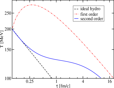
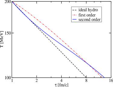
Figure 1: Temperature evolution in ideal hydrodynamics (dashed line), first order dissipative hydrodynamics (relativistic Navier-Stokes, dash-dotted line) and second order dissipative hydrodynamics (Israel-Stewart, full line), $\eta/s=0.3$. For sufficiently early initialization time $\tau_{0}$, the relativistic Navier-Stokes equation gives rise to an increase in temperature and thus total system energy, which is not seen in the Israel-Stewart theory (see text for details).

IV.1 Breakdown of hydrodynamic picture at small $\tau_{0}$

The two initial conditions used in Fig.1 are difficult to compare, since the systems differ significantly in entropy density. For the calculations in Fig. 2, we work with initial conditions for which $T_{0}^{3}\,\tau_{0}={\rm const}\sim\left(251\,{\rm MeV}\right)^{2}$. For zeroth order ideal hydrodynamics, this ensures that the choice of the initialization time $\tau_{0}$ does not affect the time evolution of the system, see (32). Irrespective of $\tau_{0}$, the system has the same entropy, and thus leads to a final state with the same event multiplicity. In this sense, the systems initialized at different $\tau_{0}$ but $T_{0}^{3}\,\tau_{0}={\rm const}$ are equivalent.

However, source gradients are larger at earlier times. Therefore, dissipative fluid dynamics will reveal stronger deviations from ideal fluid dynamics, if it is initialized at smaller $\tau_{0}$. This is seen in Fig. 2, where we plot the freeze-out time $\tau_{\rm fo}$ (defined as the time at which the system reaches $T=150$ MeV) as a function of $\tau_{0}$. For ideal fluid dynamics, the freeze-out time is unaffected by $\tau_{0}$. In the presence of dissipative effects, however, an earlier initialization provides stronger gradients and more time for deviations from ideal hydrodynamics to establish. In general, dissipative fluids take longer to cool. The larger the ratio of viscosity over entropy density $\eta/s$, the more pronounced is the effect.

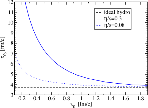
Figure 2: The freeze-out time $\tau_{\rm fo}$ (at which the system reaches $T_{\rm fo}=150$ MeV) as a function of initial time $\tau_{0}$ for ideal (dashed line) and second order dissipative hydrodynamics (solid line for $\eta/s=0.3$ and dotted line for $\eta/s=0.08$). The initial temperature $T_{0}$ was chosen such that $T_{0}^{3}\,\tau_{0}={\rm const}$, see text for details.

If the gradients in the source are too large, then the gradient expansion underlying dissipative hydrodynamics cannot be expected to converge. By estimating uncertainties in 2nd order dissipative fluid dynamics, we find that this problem becomes relevant for $\tau_{0}\raise 1.29167pt\hbox{$<$\kern-7.5pt\raise-4.73611pt\hbox{$\sim$}}1$ fm/c. At earlier times, dissipative hydrodynamics gradually loses its predictive and interpretational power.

IV.2 Breakdown of hydrodynamic picture at large $p_{T}$

The validity of a hydrodynamic picture is not only limited to sufficiently late times, but also to sufficiently low transverse momenta. To estimate the maximum transverse momentum $p_{T}^{\rm crit}$, up to which fluid dynamics may apply, we consider small departures $\delta f\ll 1$ of the phase space distribution $f$ from its equilibrium value $f_{0}$. For the gradient expansion underlying dissipative fluid dynamics to apply, one requires that local deviations $f-f_{0}$ of the phase space density are small compared to the phase space density $f$. This leads to (see Appendix A)

$$\delta f=\frac{1}{2T^{2}(\epsilon+p)}\Pi_{\mu\nu}p^{\mu}p^{\nu}\ll 1.$$ (41)

We now consider a particle at point $(\tau,\eta,r,\varphi)$, which follows the Bjorken flow, $\eta=y$, and has transverse momentum $p_{T}$. Its four-momentum reads $(p^{t},p^{x},p^{y},p^{z})=(m_{T}\cosh y,p_{T}\cos\varphi_{p},p_{T}\sin\varphi_{p},m_{T}\sinh y)$, where $m_{T}^{2}=p_{T}^{2}+m_{\rm particle}^{2}$ depends on the particle mass $m_{\rm particle}$. Averaging over the azimuthal angle $\varphi_{p}$, we find that (41) is equivalent to the condition

$$p_{T}^{2}\ll\frac{4T^{2}(\epsilon+p)}{\Phi}\,.$$ (42)

Here, $\Phi$ determines the value of the shear tensor, see (39). The dissipative strength of the system is then quantified by the inverse Reynolds number Baym

$$R_{\rm Reynolds}^{-1}=\frac{\Phi}{\epsilon+p}\,.$$ (43)

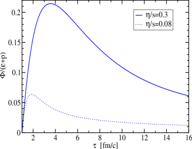
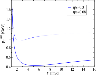
Figure 3: The time-dependence of the dissipative strength $\Phi/(\epsilon+p)$ (left plot) and the critical transverse momentum $p_{T}^{\rm crit}$ (right plot). Results are shown for initial conditions $T_{0}=300$ MeV, $\tau_{0}=1$ fm/c, and for $\eta/s=0.3$ (solid line) and $\eta/s=0.08$ (dashed line), respectively.

In Figure 3 we plot first a typical time evolution of the inverse Reynolds number $\Phi/(\epsilon+p)$ for $T_{0}=300$ MeV, $\tau_{0}=1$ fm/c and different values $\eta/s=0.3$ and $\eta/s=0.08$. Remarkably, the value for $\Phi/(\epsilon+p)$ shows a maximum at finite time. Therefore, in general, $p_{T}^{\rm crit}=\sqrt{4T^{2}(\epsilon+p)/\Phi}$ assumes its lowest value before freeze-out. Thus, the maximum $p_{T}$ at which one can still trust a hydrodynamic description may actually be lower then the apparent value obtained at freeze-out. This is shown in the second part of Fig.3, where $p_{T}^{\rm crit}$ is plotted as a function of time. As can be seen, for moderate values of $\eta/s\simeq 0.3$, one obtains a $p_{T}^{\rm crit}<0.5$ GeV.

In Fig.4, we study how the inverse Reynolds number $\Phi/(\epsilon+p)$ at the freeze-out temperature $T_{\rm fo}=150$ MeV depends on the initial conditions $\tau_{0}$ and $T_{0}$. In general, the dissipative strength increases if $\tau_{0}$ decreases or if $T_{0}$ decreases.

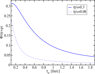
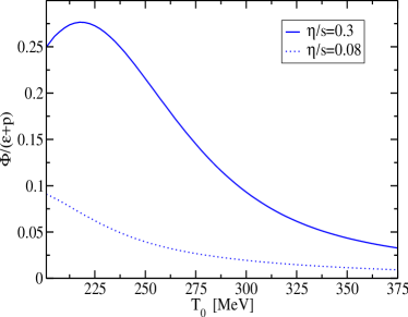
Figure 4: The dissipative strength $\Phi/(\epsilon+p)$ at freeze-out ($T_{\rm fo}=150$ MeV) as a function of initial time $\tau_{0}$ ($T_{0}=300$ MeV fixed, left plot) and as a function of initial temperature $T_{0}$ ($\tau_{0}=1$fm/c fixed, right plot) for $\eta/s=0.3$ (full lines) and $\eta/s=0.08$ (dotted lines).

IV.3 Hadron spectra at freeze-out

To calculate hadronic spectra from the phase space distribution $f$ evolved up to the freeze-out time $\tau_{\rm fo}$, one customarily makes use of the Cooper-Frye freeze-out prescription CooperFrye

$$\frac{d^{2}N}{d^{2}p_{T}dy}=\int\frac{p_{\mu}d\Sigma^{\mu}}{(2\pi)^{3}}f\,.$$ (44)

Here, $d\Sigma_{\mu}$ denotes the oriented freeze-out volume. For the case of a Bjorken one-dimensional expansion, $p_{\mu}d\Sigma^{\mu}=m_{T}\cosh(y-\eta)\tau d\eta rdrd\phi$. We now consider a phase space distribution $f$ at freeze-out, that deviates locally from equilibrium $f_{0}$. Adopting the ansatz of Ref. Teaney , which embeds information about dissipative effects directly in the freeze-out distribution, we write

$$f=f_{0}\left(1+\frac{1}{2T^{2}(\epsilon+p)}\Pi_{\mu\nu}p^{\mu}p^{\nu}\right)\,.$$ (45)

Since the relation (44) between the particle spectrum and the phase space distribution is linear, this allows us to define the particle spectrum in terms of its ideal part and its dissipative corrections. Specializing to the case of a Boltzmann distribution $f_{0}(p_{\mu}u^{\mu})=2(N_{c}^{2}-1)\,\exp(-p_{\mu}u^{\mu}/T)$, one finds for the ideal partSchnedermann

$$\frac{d^{2}N^{0}}{d^{2}p_{T}dy} = \int\frac{p_{\mu}d\Sigma^{\mu}}{(2\pi)^{3}}f_{0}$$ (46)

$$= 2(N_{c}^{2}-1)m_{T}\tau_{\rm fo}\frac{R_{0}^{2}}{(2\pi)^{2}}K_{1}\left(\frac{m_{T}}{T}\right)\,.$$

The total yield is proportional to the transverse area $\pi\,R_{0}^{2}$ over which we have integrated. For numerical calculations, we use $R_{0}=6$ fm. For a Boltzmann distribution and longitudinally boost-invariant flow, the dissipative correction to this spectrum reads

$$\frac{d^{2}\delta N}{d^{2}p_{T}dy} = \frac{\Pi_{\alpha\beta}}{2T^{2}(\epsilon+p)}\int\frac{p_{\mu}d\Sigma^{\mu}}{(2\pi)^{3}}f_{0}p^{\alpha}p^{\beta}.$$ (47)

$$= \frac{\Phi}{4(\epsilon+p)}\frac{2(N_{c}^{2}-1)m_{T}\tau_{\rm fo}R_{0}^{2}}{(2\pi)^{2}}\left[\left(\frac{p_{T}}{T}\right)^{2}K_{1}\left(\frac{m_{T}}{T}\right)\right.$$

$$\qquad\qquad\left.-\frac{1}{2}\left(\frac{m_{T}}{T}\right)^{2}\left(K_{3}\left(\frac{m_{T}}{T}\right)-K_{1}\left(\frac{m_{T}}{T}\right)\right)\right].$$

If $\eta/s$ is very small then dissipative corrections will be small. For instance, for the small value $\eta/s=0.08$, one finds a small dissipative strength $\Phi/(\epsilon+p)\sim 0.02$ at freeze-out, if one uses $\tau_{0}>0.8$ fm/c and $T_{0}>300$ MeV for the initial conditions (see Fig.4). This estimate can be reconciled with the discussion in Ref. Teaney , if one uses $\tau_{\rm fo}\sim 9$ fm/c and $T_{\rm fo}\sim 150$ MeV so that $\tau_{\rm fo}T_{\rm fo}\sim 7$ instead of $\tau_{\rm fo}T_{\rm fo}\sim 1$ used in Teaney . For this small dissipative strength, we expect only slight modifications of hadron spectra. This is confirmed in Fig.5.

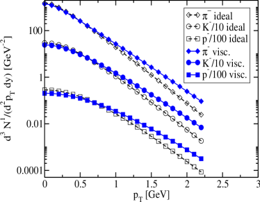
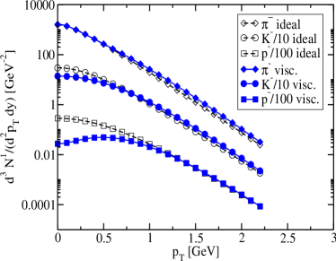
Figure 5: Particle spectra for pions, kaons and protons from ideal hydrodynamics (open symbols) and viscous hydrodynamics (full symbols), for $R_{0}=6$ fm/c. Left plot: spectra from ideal and viscous hydrodynamics ($\Phi/(\epsilon+p)=0.02$) for the same freeze-out conditions. Right plot: spectra for ideal and viscous hydrodynamics ($\Phi/(\epsilon+p)=0.05$) with freeze-out of the ideal case adjusted such that slope of viscous calculation is reproduced at intermediate $p_{T}$, (see text for details).

However, freeze-out time $\tau_{\rm fo}$ and temperature $T_{\rm fo}$ are not directly measurable. Rather, they are intrinsic parameters of the hydrodynamic model and its possible matching to a hadronic rescattering phase. This raises the question to what extent dissipative effects can be accommodated in an ideal fluid description of data by varying the freeze-out conditions of the ideal fluid. In Fig. 5, we have calculated hadronic spectra $N^{1}=N^{0}+\delta N$ for a sizable dissipative strength $\Phi/(\epsilon+p)=0.05$ and freeze-out conditions $(\tau_{\rm fo},T_{\rm fo})=(14{\rm fm/c},140MeV)$. Remarkably, these spectra can be reproduced to a significant degree by an ideal fluid model, using the same initialization but a different decoupling time and temperature $(\tau_{\rm fo},T_{\rm fo})=(17{\rm fm/c},170MeV)$. The only clearly visible difference between both models in Fig. 5 is a characteristic mass-dependent dip in the low-$p_{\perp}$ part of the spectrum which increases with increasing dissipative strength. This dip is a direct consequence of the analytical form (47), and appears to be rather sensitive to small values of the inverse Reynolds number. We have observed with curiosity that the fine-binned data available from BRAHMS Ouerdane:2002gm for $p_{\perp}>0.5$ GeV for anti-protons maybe hints a similar dip around the lower end of the experimental reach. We regard this as an illustration that improved particle-identified measurements of hadronic transverse momentum spectra in the non-relativistic momentum regime (e.g. smaller error bars from PHOBOS Wosiek:2002ur ) may provide valuable constraints for dissipative properties of the produced dense matter.

V Conclusions

The predictive and interpretational power of fluid dynamics simulations relies on knowledge about the initial conditions, the dissipative properties during evolution, and the modeling of decoupling in the final state, all of which are accompanied by significant uncertainties in phenomenological applications. This raises the question to what extent information about fundamental dissipative properties of dense QCD matter can be constrained experimentally in heavy ion collisions. To address this question, we have compared here results from ideal and dissipative fluid dynamics.

First, from Boltzmann transport theory (see Section II and Appendices), we have established that derivations of second order hydrodynamics based on the implementation of $d_{\mu}s^{\mu}\geq 0$, (18) do not provide the complete set of second order terms in a gradient expansion. They discard those terms in the gradient expansion which are orthogonal to the shear viscous tensor. We then explored in a model study the region of applicability of fluid dynamics. We found that for too early initialization times $\tau_{0}\raise 1.29167pt\hbox{$<$\kern-7.5pt\raise-4.73611pt\hbox{$\sim$}}1$ fm/c, source gradients are too large for dissipative hydrodynamics to converge (see Figs. 1 and  2). The inverse Reynolds number $\Phi/(\epsilon+p)$ defines a useful $p_{T}$-dependent scale $p_{T}^{\rm crit}$ up to which dissipative hydrodynamics can be expected to account for deviations from the local equilibrium of a perfect fluid. For our model, we found typically a $p_{T}^{\rm crit}\raise 1.29167pt\hbox{$<$\kern-7.5pt\raise-4.73611pt\hbox{$\sim$}}1$ GeV.

Once we had delineated for our model the range of validity of a fluid dynamics description, we asked whether data taken within this range can be interpreted unambiguously in terms of the strength of dissipative properties of matter. Our results illustrate the challenges of this task. While even for a very small dissipative strength, model calculations of transverse hadron spectra show a measurable sensitivity to dissipative properties, a very good control over initial conditions and freeze-out is required to extract these features from data. In particular, in our model hadronic spectra including sizeable dissipative effects could be reproduced rather satisfactorily from perfect fluid calculations by modifying the freeze-out temperature and time (see Fig. 5).

The fluid dynamics model studied here is based on a strongly simplified transverse geometry and does not account for a hadronic scattering phase. Therefore, this setup does not exhibit all characteristic features of a realistic heavy ion collision, such as transverse radial and elliptic flow. However, the two-step logic used here to assess the range of validity and the interpretational power of our model applies also to the more complex, realistic fluid dynamics simulations of heavy ion collisions: First, a comparison of ideal and dissipative fluid dynamics results delineates the range of validity of a fluid dynamics description. Second, within this limited range, one has to establish by model studies to what extent conclusions about the equation of state or dissipative properties are independent of the initial conditions and the modeling of the freeze-out. For more complex models, there are more measurable quantities (such as elliptic flow), which may help to constrain the fluid dynamics. However, there are also more features of the initial conditions, which require specification (such as the initial transverse density and flow profile). This increases the complexity of the task to disentangle effects of initial conditions from those of the properties of matter determining fluid dynamics behavior. We expect that the numerical values for the bounds on initialization time and transverse momentum of a reliable fluid description, established here, change only weakly by going to more complex fluid simulations.

Appendix A Dissipative hydrodynamics from kinetic theory: Derivation for a massless Boltzmann gas

In this Appendix, we derive the equation of motion (3) of dissipative hydrodynamics from kinetic theory for a massless Boltzmann gas. Our starting point is the Boltzmann transport equation

$$p^{\mu}d_{\mu}f({\bf x},t,{\bf p})={\mathcal{C}}(x)\,,$$ (48)

with ${\mathcal{C}}$ the collision term. We make use of the notational shorthands (4)-(11). We consider the first three moments of the Boltzmann equation (48), using $\int d\omega\equiv\int\frac{d^{3}p}{(2\pi)^{3}\,p_{0}}$

$$\int\ d\omega p^{\mu}d_{\mu}f=d_{\mu}N^{\mu}= 0 =\int d\omega\ {\mathcal{C}}\,,$$ (49)

$$\int d\omega\ p^{\mu}p^{\alpha}d_{\mu}f=d_{\mu}T^{\mu\alpha}= 0 =\int d\omega\ p^{\alpha}{\mathcal{C}}\,,$$ (50)

$$\int d\omega\ p^{\mu}p^{\alpha}p^{\beta}d_{\mu}f = \int d\omega\ p^{\alpha}p^{\beta}{\mathcal{C}}\,.$$ (51)

Here, equations (49) and (50) stand for charge conservation and energy-momentum conservation, respectively. Equation (51) is the lowest order relation of moments of (48), which contains dynamic information. For simplicity, we consider in the following an equilibrium distribution $f_{0}$ of the Boltzmann type for one degree of freedom, $f_{0}(u_{\mu}p^{\mu})=\exp(-\beta u_{\mu}p^{\mu})$. Also, we employ the relaxation time approximation in Eq.(51),

$${\mathcal{C}}=-p_{\mu}u^{\mu}\frac{f-f_{0}}{\tau_{\Pi}}\,.$$ (52)

For all points $({\bf x},t,{\bf p})$ in phase space, where we want a hydrodynamic description to apply, we assume that departures from local equilibrium are small,

$$f=f_{0}(1+\delta f)\,.\qquad|\delta f|\ll 1$$ (53)

The correction term $\delta f$ can be written in the form

$$\delta f({\bf x},t,{\bf p})=\epsilon({\bf x},t)+\epsilon_{\lambda}({\bf x},t)p^{\lambda}+\epsilon_{\lambda\nu}({\bf x},t)p^{\lambda}p^{\nu}.$$ (54)

The deviations from the equilibrium energy-momentum tensor $T^{\mu\nu}_{0}$ can be likewise written as

$$T^{\mu\nu}=T^{\mu\nu}_{0}+\Pi^{\mu\nu}+\Pi\Delta^{\mu\nu}+q^{(\mu}u^{\nu)}\,.$$ (55)

Here, the deviations from local equilibrium due to shear viscosity, bulk viscosity and heat flow are parametrized by $\Pi^{\mu\nu}$, $\Pi$ and $q^{\mu}$, respectively. We limit the following discussion to the effects of shear viscosity, which is expected to provide for the most significant dissipative effects. It can be shown IS that in this case we may ignore both the zeroth and first order term in $p$ in Eq.(54) as well as concentrate on $T^{<\mu\nu>}$ only. We are left with $\delta f({\bf x},t,{\bf p})=\epsilon_{\lambda\nu}({\bf x},t)p^{\lambda}p^{\nu}$, so that the second moment of the Boltzmann equation reads

$$d_{\mu}\int d\omega p^{\mu}p^{<\alpha}p^{\beta>}f_{0}\left(1+\epsilon_{\gamma\delta}p^{\gamma}p^{\delta}\right)=-\frac{\epsilon_{\gamma\delta}u_{\epsilon}}{\tau_{\Pi}}\int d\omega p^{<\alpha}p^{\beta>}p^{\gamma}p^{\delta}p^{\epsilon}f_{0}\,.$$ (56)

To derive from this expression the equation of motion for the non-equilibrium deviation $\Pi_{\mu\nu}$ of the energy momentum tensor, we establish first the relation between $\epsilon_{\mu\nu}$ and $\Pi_{\mu\nu}$. We start from

$$<T^{\mu\nu}-T^{\mu\nu}_{0}> = \int d\omega p^{<\mu}p^{\nu>}(f-f_{0})$$ (57)

$$= \epsilon_{\alpha\beta}(x)\int d\omega p^{<\mu}p^{\nu>}p^{\alpha}p^{\beta}f_{0}$$

$$= \epsilon_{\alpha\beta}(x)I^{<\mu\nu>\alpha\beta}\,,$$

where

$$I^{\mu_{1}\mu_{2}\ldots\mu_{n}}\equiv\int d\omega p^{\mu_{1}}p^{\mu_{2}}\ldots p^{\mu_{n}}f_{0}\,.$$ (58)

For the Boltzmann distribution $f_{0}=\exp{(-p_{\mu}u^{\mu}/T)}$, the integral (58) can be solved analytically for general $n$ IS . In the following, we need the cases $n=4,5$ which read

$$I^{\mu\nu\alpha\beta} = a_{0}u^{\mu}u^{\nu}u^{\alpha}u^{\beta}+a_{1}\left(\Delta^{\mu\nu}u^{\alpha}u^{\beta}+perm\right)$$ (59)

$$+a_{2}\left(\Delta^{\mu\nu}\Delta^{\alpha\beta}+\Delta^{\mu\alpha}\Delta^{\nu\beta}+\Delta^{\mu\beta}\Delta^{\alpha\nu}\right)\,,$$

$$I^{\mu\nu\alpha\beta\gamma} = b_{0}u^{\mu}u^{\nu}u^{\alpha}u^{\beta}u^{\gamma}+b_{1}\left(\Delta^{\mu\nu}u^{\alpha}u^{\beta}u^{\gamma}+perm.\right)$$ (60)

$$+b_{2}\left(\Delta^{\mu\nu}\Delta^{\alpha\beta}u^{\gamma}+perm.\right)\,.$$

The temperature dependent coefficients $a_{i}$ and $b_{i}$ in (59) and (60) can be calculated e.g. by going to the fluid rest-frame, $u^{\mu}=(1,{\bf 0})$. One finds $a_{2}=4T^{6}/\pi^{2}$ and $b_{2}=24T^{7}/\pi^{2}$. The first of these coefficients is related to the pressure $p$ and energy density $\epsilon$ as $a_{2}=T^{2}(\epsilon+p)$. Combining Eqs. (55), (57) and (59), we find

$$\epsilon_{\alpha\beta}(x)I^{<\mu\nu>\alpha\beta} = 2a_{2}\epsilon_{\alpha\beta}\Delta^{\alpha<\mu}\Delta^{\nu>\beta}$$ (61)

$$= 2\Pi^{\mu\nu}=\Pi^{<\mu\nu>}\,.$$

This equation implies $u_{\mu}\Pi^{\mu\nu}=0$ and $\Delta_{\mu\nu}\Pi^{\mu\nu}=0$. Therefore, we can set

$$\epsilon^{\mu\nu}=\frac{1}{2a_{2}}\Pi^{\mu\nu}\,.$$ (62)

This allows us to rewrite Eq.(56) as

$$d_{\mu}\left(I^{\mu<\alpha\beta>}+\epsilon_{\gamma\delta}I^{\mu<\alpha\beta>\gamma\delta}\right)=-\frac{\epsilon_{\gamma\delta}u_{\epsilon}}{\tau_{\Pi}}I^{<\alpha\beta>\gamma\delta\epsilon}$$ (63)

The three terms entering this equation can be rewritten with the help of the identities derived above,

$$\epsilon_{\gamma\delta}u_{\epsilon}I^{<\alpha\beta>\gamma\delta\epsilon}=2b_{2}\epsilon_{\gamma\delta}\Delta^{\gamma<\alpha}\Delta^{\beta>\delta}=\frac{b_{2}}{a_{2}}\Pi^{<\alpha\beta>}\,,$$ (64)

$$d_{\mu}\int d\omega p^{\mu}p^{<\alpha}p^{\beta>}f_{0}=-I^{\mu<\alpha\beta>\gamma}d_{\mu}\frac{u_{\gamma}}{T}=-\frac{2a_{2}}{T}<\nabla^{\alpha}u^{\beta}>\,,$$ (65)

$$I^{\mu<\alpha\beta>\gamma\delta}d_{\mu}\epsilon_{\gamma\delta}=2b_{2}\left(\Delta^{\gamma<\alpha}\Delta^{\beta>\delta}u^{\mu}d_{\mu}\epsilon_{\gamma\delta}+2u^{\gamma}\Delta^{\mu<\alpha}\Delta^{\beta>\delta}d_{\mu}\epsilon_{\gamma\delta}\right)\,.$$ (66)

Further simplifications arise from $u^{\gamma}d_{\mu}\Pi_{\gamma\delta}=-\Pi_{\gamma\delta}d_{\mu}u^{\gamma}$ and $\Delta_{\gamma\delta}d_{\mu}\Pi^{\gamma\delta}=d_{\mu}\Delta_{\gamma\delta}\Pi^{\gamma\delta}=0$. We then decompose $\Pi^{\mu\nu}d_{\mu}u_{\nu}$ into a totally symmetric component $\propto\theta_{\mu\nu}$, and a totally antisymmetric expression proportional to the vorticity tensor $\omega_{\nu\mu}$

$$\Pi^{\gamma\delta}d_{\mu}u_{\gamma} = \Pi^{\gamma\delta}(\omega_{\gamma\mu}+\theta_{\gamma\mu})\,,$$ (67)

$$\omega^{\mu\nu} = \Delta^{\mu\alpha}\Delta^{\nu\beta}d_{[\beta}u_{\alpha]}\,,$$ (68)

$$\theta^{\mu\nu} = \Delta^{\mu\alpha}\Delta^{\nu\beta}d_{(\beta}u_{\alpha)}\,.$$ (69)

At this point, we follow IS in assuming the ’rigidity of flow’. This means that one assumes the equilibrium flow $u^{\mu}$ to be shear free, and thus terms proportional to $\theta^{\mu\nu}$ to vanish. As a consequence, the term $\epsilon_{\gamma\delta}\int d\omega p^{\mu}p^{<\alpha}p^{\beta>}p^{\gamma}p^{\delta}d_{\mu}f_{0}$ can be neglected. Then, Eq.(63) reads

$$\frac{-a_{2}}{T}<\nabla^{\alpha}u^{\beta}>+\frac{b_{2}}{a_{2}}\left(\Delta^{\gamma\alpha}\Delta^{\beta\delta}D\Pi_{\gamma\delta}+2\Pi^{\delta(\alpha}\omega^{\beta)}_{\ \delta}\right)+b_{2}\Pi^{\alpha\beta}Da_{2}^{-1}=-\frac{1}{\tau_{\Pi}}\frac{b_{2}}{a_{2}}\Pi^{\alpha\beta}.$$ (70)

For the third term on the left hand side, $Da_{2}^{-1}\propto D\epsilon\propto d_{\mu}u^{\mu}\propto\theta_{\mu}^{\mu}$, which vanishes under the assumption of rigid flow. We note that in Ref. Muronga ; Muronga:2004sf , this term is kept. The contractions $u_{\nu}d_{\mu}T^{\mu\nu}=0$ and $\Delta_{\nu\alpha}d_{\mu}T^{\mu\nu}=0$ for an energy momentum tensor of the form $T^{\mu\nu}=T^{\mu\nu}_{0}+\Pi^{\mu\nu}$ lead to the equations of motion (1) and (2), respectively. To complete the derivation of (3), we require that in the limit $\tau_{\Pi}\to 0$, the first order dissipative Navier-Stokes equations are recovered from (70). This leads to the identification

$$\frac{a_{2}^{2}}{Tb_{2}}\rightarrow\eta/\tau_{\Pi}\,.$$ (71)

The equation of motion (3) then follows from (70).

Appendix B Dissipative Hydrodynamics: Derivation for a massless Bose-Einstein gas and momentum-dependent relaxation time

In this Appendix we derive the second order hydrodynamic equation (3) for the case that the relaxation time $\tau_{\Pi}$ is momentum-dependent, $\tau_{\Pi}=p_{\mu}u^{\mu}\hat{\tau}$, $\hat{\tau}={\rm const}$. This ansatz is of interest since it often enters calculations of the shear viscosity (see Refs. visc ; relax ; Heiselberg and sec. 8.3 of the textbook LeBellac ). In contrast to Appendix A, we start here from the equilibrium distribution for a massless Bose-Einstein gas $f_{0}=[\exp(\beta u_{\mu}p^{\mu})-1]^{-1}$, having in mind QCD with gluonic degrees of freedom. This implies that the departures from equilibrium are expressed by [c.f. Eq.(53)]

$$\delta f({\bf x},t,{\bf p})=(1+f_{0})\epsilon_{\lambda\nu}({\bf x},t)p^{\lambda}p^{\nu}\,.$$ (72)

The relation between $\epsilon_{\mu\nu}$ and $\Pi_{\mu\nu}$ is expressed as in Eq.(62), except that the coefficient $a_{2}$ is replaced by $\hat{a}_{2}=4\zeta(5)T^{6}/\pi^{2}$, with $\zeta(n)$ the Riemann $\zeta$-function. This implies that $\hat{a}_{2}=\frac{\zeta(5)}{\zeta(4)}T^{2}(\epsilon+p)$ when expressed in terms of energy density and pressure of the free Bose-Einstein gas. This modification, compared to the Boltzmann gas used in App.A, is due to the replacement of the integrals $I^{\mu_{1}\mu_{2}\ldots\mu_{n}}$ by

$${\hat{I}}^{\mu_{1}\mu_{2}\ldots\mu_{n}}=\int d\omega p^{\mu_{1}}p^{\mu_{2}}\ldots p^{\mu_{n}}f_{0}(1+f_{0})\,.$$ (73)

The second moment of the Boltzmann equation (48) reads now

$$d_{\mu}\left(I^{\mu<\alpha\beta>}+\epsilon_{\gamma\delta}\hat{I}^{\mu<\alpha\beta>\gamma\delta}\right)=-\frac{\epsilon_{\gamma\delta}}{\hat{\tau}}\hat{I}^{<\alpha\beta>\gamma\delta}\,,$$ (74)

where the right hand side depends on an order four tensor only, in contrast to the order five tensor entering Eq.(63). Consequently, for a Bose-Einstein gas we find

$$d_{\mu}I^{\mu\langle\alpha\beta\rangle} = -\frac{2\hat{a}_{2}}{T}\langle\nabla^{\alpha}u^{\beta}\rangle\,,$$ (75)

$$\epsilon_{\gamma\delta}\hat{I}^{<\alpha\beta>\gamma\delta} = \Pi_{\gamma\delta}\Delta^{\gamma<\alpha}\Delta^{\beta>\delta}=2\Pi^{\alpha\beta}\,,$$ (76)

$$\hat{I}^{\mu<\alpha\beta>\gamma\delta}d_{\mu}\epsilon_{\gamma\delta} = 2\hat{b}_{2}\left(\Delta^{\gamma<\alpha}\Delta^{\beta>\delta}u^{\mu}d_{\mu}\epsilon_{\gamma\delta}+2u^{\gamma}\Delta^{\mu<\alpha}\Delta^{\beta>\delta}d_{\mu}\epsilon_{\gamma\delta}\right)\,,$$ (77)

where

$$\hat{b}_{2}=\frac{24}{\pi^{2}}\zeta(6)T^{7}\,.$$ (78)

Together with the assumption of the “rigidity of flow”, i.e. setting $\theta_{\mu\nu}\equiv 0$, Eq.(74) becomes

$$\frac{-\hat{a}_{2}}{T}<\nabla^{\alpha}u^{\beta}>+\frac{\hat{b}_{2}}{\hat{a}_{2}}\left(\Delta^{\gamma\alpha}\Delta^{\beta\delta}D\Pi_{\gamma\delta}+2\Pi^{\delta(\alpha}\omega^{\beta)}_{\ \delta}\right)=-\frac{1}{\hat{\tau}}\frac{\hat{b}_{2}}{\hat{a}_{2}}\Pi^{\alpha\beta}.$$ (79)

Thus, we recover Eq. (3) upon identifying

$$\eta\leftrightarrow\frac{\hat{a}_{2}}{T}\hat{\tau},\quad\tau_{\Pi}\leftrightarrow\frac{\hat{b}_{2}}{\hat{a}_{2}}\hat{\tau},$$ (80)

which leads to the ratio

$$\beta_{2}=\frac{\hat{b}_{2}T}{2(\hat{a}_{2})^{2}}=\frac{3}{4p}\frac{\zeta(4)\zeta(6)}{\zeta(5)^{2}}\simeq 1.024\frac{3}{4p}\,.$$ (81)

In conclusion, the dissipative hydrodynamic equations for a massless Boltzmann and Bose-Einstein gas differ, but only on the order of a few percent.

Appendix C Perturbative calculation of the relaxation time

To complete the discussion on viscosity and relaxation time, we calculate in QCD the relaxation time $\hat{\tau}=\tau_{\Pi}(p_{\mu}u^{\mu})^{-1}$ to leading order in the strong coupling constant $g$. We follow the line of argument of Refs.visc ; Heiselberg ; LeBellac for a gluonic system with $2(N_{c}^{2}-1)=16$ degrees of freedom. The collision term $\mathcal{C}$, entering this calculation, is then dominated by $2\leftrightarrow 2$ gluon scattering processes. The corresponding effective matrix element $M_{gg}$ is given in the hard-thermal loop (HTL) approximation, including Landau damping LeBellac . To simplify the calculation, a small time-independent velocity $u^{x}(y)$ is considered which only varies with the space coordinate $y$ visc ,

$$p_{\mu}d^{\mu}f({\bf x},t,{\bf p})\simeq-f_{0}(1+f_{0})\frac{p^{x}p^{y}}{T}\beta\frac{\partial u^{x}(y)}{\partial y}\,.$$ (82)

Following analogous steps as in visc ; LeBellac , $\hat{\tau}$ can be written in terms of the ratio

$$\frac{1}{\hat{\tau}} = \frac{2(N_{c}^{2}-1)}{16}\left[\prod_{i=1}^{4}\int d\omega_{i}(2\pi)^{4}\delta^{4}(p_{1}+p_{2}-p_{3}-p_{4})\overline{|M_{gg}|^{2}}(p_{1}^{x}p_{1}^{y})^{2}f_{0}(p_{1})\right.$$ (83)

$$\left.\times f_{0}(p_{2})\left(1+f_{0}(p_{3})\right)\left(1+f_{0}(p_{4})\right)\right]/\left(\int d\omega(p^{x}p^{y})^{2}f_{0}(1+f_{0})\right)\,.$$

Here, $\overline{|M_{gg}|^{2}}$ denotes the scattering matrix element squared, summed (averaged) over spins and color degrees of freedom in the final (initial) state. The integrals are evaluated e.g. in LeBellac , leading to

$$\frac{1}{\hat{\tau}}=\frac{(N_{c}^{2}-1)\pi^{5}T^{2}}{120\ \zeta(5)}\frac{g^{4}}{(4\pi)^{2}}\ln(4\pi/g^{2})\,.$$ (84)

From Eq.(80), the estimate for $\eta$ is derived

$$\eta=\frac{\hat{a}_{2}}{T}\hat{\tau}=\frac{960}{\pi^{7}}\zeta^{2}(5)T^{3}\frac{(4\pi)^{2}}{g^{4}\ln(4\pi/g^{2})},$$ (85)

when taking the color degrees of freedom into account. We note that $\hat{a}_{2}$ is proportional to a factor $2(N_{c}^{2}-1)$. This expression agrees also with the value quoted in Trans1 .

References

- (1) K. Adcox et al. [PHENIX Collaboration], Nucl. Phys. A 757 (2005) 184.
- (2) B. B. Back et al. [PHOBOS Collaboration], Nucl. Phys. A 757 (2005) 28.
- (3) I. Arsene et al. [BRAHMS Collaboration], Nucl. Phys. A 757 (2005) 1.
- (4) J. Adams et al. [STAR Collaboration], Nucl. Phys. A 757 (2005) 102.
- (5) P. Danielewicz and M. Gyulassy, Phys. Rev. D 31 (1985) 53.
- (6) P. Arnold, G. D. Moore and L. G. Yaffe, JHEP 0011 (2000) 001.
- (7) P. Arnold, G. D. Moore and L. G. Yaffe, JHEP 0305 (2003) 051.
- (8) G. Policastro, D. T. Son and A. O. Starinets, Phys. Rev. Lett. 87 (2001) 081601.
- (9) H. Heiselberg, Phys. Rev. D 49 (1994) 4739; G. Baym, H. Monien, C. J. Pethick and D. G. Ravenhall, Phys. Rev. Lett. 64 (1990) 1867.
- (10) D. Teaney, J. Lauret and E. V. Shuryak, Phys. Rev. Lett. 86 (2001) 4783.
- (11) P. Huovinen, P. F. Kolb, U. W. Heinz, P. V. Ruuskanen and S. A. Voloshin, Phys. Lett. B 503 (2001) 58.
- (12) P. F. Kolb, U. W. Heinz, P. Huovinen, K. J. Eskola and K. Tuominen, Nucl. Phys. A 696 (2001) 197.
- (13) T. Hirano and K. Tsuda, Phys. Rev. C 66, 054905 (2002).
- (14) P. F. Kolb and R. Rapp, Phys. Rev. C 67, 044903 (2003).
- (15) K. H. Ackermann et al. [STAR Collaboration], Phys. Rev. Lett. 86 (2001) 402.
- (16) K. Adcox et al. [PHENIX Collaboration], Phys. Rev. Lett. 89 (2002) 212301.
- (17) S. S. Adler et al. [PHENIX Collaboration], Phys. Rev. Lett. 91 (2003) 182301.
- (18) S. S. Adler et al. [PHENIX Collaboration], Phys. Rev. C 69 (2004) 034909.
- (19) J. Adams et al. [STAR Collaboration], Phys. Rev. Lett. 92 (2004) 112301.
- (20) U. W. Heinz, AIP Conf. Proc. 739 (2005) 163.
- (21) R. Baier, A. H. Mueller, D. Schiff and D. T. Son, Phys. Lett. B 539 (2002) 46.
- (22) D. Molnar and M. Gyulassy, Nucl. Phys. A 697 (2002) 495 [Erratum-ibid. A 703 (2002) 893].
- (23) E. V. Shuryak, Nucl. Phys. A 750 (2005) 64.
- (24) T. D. Lee, Nucl. Phys. A 750 (2005) 1.
- (25) M. Gyulassy and L. McLerran, Nucl. Phys. A 750 (2005) 30.
- (26) U. W. Heinz, arXiv:nucl-th/0512051.
- (27) B. Muller and J. L. Nagle, arXiv:nucl-th/0602029.
- (28) S. K. Blau, Phys. Today 58N5 (2005) 23.
- (29) S. Mrowczynski, Phys. Lett. B 393 (1997) 26.
- (30) P. Arnold, J. Lenaghan, G. D. Moore and L. G. Yaffe, Phys. Rev. Lett. 94 (2005) 072302.
- (31) A. Rebhan, P. Romatschke and M. Strickland, Phys. Rev. Lett. 94 (2005) 102303.
- (32) A. Dumitru and Y. Nara, Phys. Lett. B 621 (2005) 89.
- (33) P. Romatschke and R. Venugopalan, Phys. Rev. Lett. 96, (2006) 062302.
- (34) T. Hirano, U. W. Heinz, D. Kharzeev, R. Lacey and Y. Nara, arXiv:nucl-th/0511046.
- (35) R. S. Bhalerao, J. P. Blaizot, N. Borghini and J. Y. Ollitrault, Phys. Lett. B 627 (2005) 49.
- (36) W. Israel, Ann.Phys. 100 (1976) 310; W. Israel and J.M. Stewart, Phys. Lett. 58A (1976) 213; W. Israel and J.M. Stewart, Ann.Phys. 118, (1979) 341.
- (37) A. Muronga, Phys. Rev. Lett. 88 (2002) 062302 [Erratum-ibid. 89 (2002) 159901]; Phys. Rev. C 69 (2004) 034903.
- (38) A. Muronga and D. H. Rischke, arXiv:nucl-th/0407114.
- (39) A. K. Chaudhuri and U. W. Heinz, arXiv:nucl-th/0504022; U. W. Heinz, H. Song and A. K. Chaudhuri, arXiv:nucl-th/0510014.
- (40) M. Prakash, M. Prakash, R. Venugopalan and G. M. Welke, Phys. Rev. Lett. 70 (1993) 1228 [Nucl. Phys. A 566 (1994) 403c].
- (41) M. Prakash, M. Prakash, R. Venugopalan and G. Welke, Phys. Rept. 227 (1993) 321.
- (42) W.A. Hiscock and L. Lindblom, Phys. Rev. D 31, 725 (1985).
- (43) F. Cooper and G. Frye, Phys. Rev. D 10, 186 (1974).
- (44) D. H. Rischke, arXiv:nucl-th/9809044, Hadrons in Dense Matter and Hadrosynthesis, ed. by J.Cleymans, H.B. Geyer and F.G. Scholz, Springer Lecture Notes in Physics 516, 21 (1999).
- (45) J. Bjorken, Phys. Rev. D 27, 140 (1983).
- (46) H. Kouno, M. Maruyama, F. Takagi and K. Saito, Phys. Rev. D 41 (1990) 2903.
- (47) Y. Lallouet, D. Davesne and C. Pujol, Phys. Rev. C 67 (2003) 057901.
- (48) G. Baym, Nucl. Phys. A 418 (1984) 525c.
- (49) D. Teaney, Phys. Rev. C 68 (2003) 034913.
- (50) E. Schnedermann, J. Sollfrank and U. W. Heinz, Phys. Rev. C 48 (1993) 2462.
- (51) D. Ouerdane [BRAHMS Collaboration], Nucl. Phys. A 715 (2003) 478.
- (52) B. Wosiek et al. [PHOBOS Collaboration], Nucl. Phys. A 715 (2003) 510.
- (53) G. Baym, Phys. Lett. B 138 (1984) 18; A. Hosoya and K. Kajantie, Nucl. Phys. B 250 (1985) 666.
- (54) H. Heiselberg and X. N. Wang, Nucl. Phys. B 462 (1996) 389.
- (55) M. LeBellac, “Thermal Field Theory”, Cambridge University Press (1996)