Coupling constants and transition potentials for hadronic decay modes of a meson

Abstract

Within the independent-harmonic-oscillator model for quarks inside a hadron, a rigorous method is presented for the calculation of coupling constants and transition potentials for hadronic decay, as needed in a multi-channel description of mesons.

1 Introduction

In several publications [1, 2, 3, 4] it is discussed that hadronic decay cannot be ignored in hadron models. As a consequence it is essential for the description of mesons (and baryons) to know the allowed decay modes and their relative strengths.

The use of independent harmonic oscillators for the calculation of the angular-momentum part of rearrangement matrix elements, has been demonstrated in a previous paper [5]. There it was shown that the difficulties, which arise in naive recoupling schemes [6] when for a decay process the decay products have internal angular excitations, can easily be handled once one introduces explicit wave functions for the partons involved. This fact has already been elaborated in [7] and [8] and successfully applied to the calculation of branching ratios for the decay of mesons. Here we want to use this as a method for determining the coupling constants and transition potentials in a multichannel meson-meson scattering model [9, 10].

There is, however, in principle no limit on the number of possible decay modes in the schemes of Refs. [7, 8]. For this reason we prefer the rearrangement method of [5]. Essentially, when one wants to calculate all possible decay channels of a given initial state, then the harmonic-oscillator treatment has the advantage that there is only finite number of possible decay channels involved, which in a certain sense is complete. As a consequence, one can always easily verify whether all possibilities are taken into account.

In this paper we will calculate explicitly the matrix elements for the decay processes:

$${\textstyle\mbox{\rm meson}}\;\to\;{\textstyle\mbox{\rm meson}}+{\textstyle\mbox{\rm meson}}$$

(Sects. 2, 3, 4). Of course, the Clebsch-Gordannery is straightforward, but it is useful to have the complete formulas written somewhere. Moreover, the here presented strategy is not totally trivial. We will see that in order to obtain the proper selection rules for the decay products, we only need to impose Fermi statistics on the quarks and the antiquarks. $G$ parity is then automatically obeyed. In Sect. 5 some of the resulting coupling constants are compared to the data. The construction of a transition potential which can be used in models [9, 10] for the description of hadronic decay, is given in Sect. 6.

2 The meson just before decay

Just before decay a meson is assumed to consist of four partons in the ${{}^{3}P_{0}}$ model (see also Fig. 1):

1. the original quark-antiquark ($q\bar{q}$) pair which carries all the quantum numbers of the decaying meson,

2. the newly created $q\bar{q}$ pair with the quantum numbers of the vacuum ($J^{PC}=0^{++}$).

Figure 1: The four-quark system of the original pair and the newly created ${{}^{3}P}_{0}$ pair, just before decay.

First we introduce a quarkspinor which describes a quark with flavorindex $a$ (here the number of flavors is restricted to three; the generalization to more flavors is straightforward), colorindex $\alpha$ and spin magnetic quantum number $\mu$ by

$$q^{a}_{\alpha}\left(\mu\right)\;\;\;.$$ (1)

For an antiquark we use similarly the notation

$$\bar{q}^{\,\alpha}_{a}\left(\mu\right)\;\;\;.$$ (2)

The wave function describing the system of four partons which compose a decaying meson, is the product of two parts:

1. The wave function of the original $q\bar{q}$ pair, which consists of a color-singlet quark-antiquark pair with (flavor, spin) indices ($a$, $\mu_{1}$) for the quark and ($b$, $\mu_{2}$) for the antiquark

   $$\mbox{\raisebox{2.15277pt}{$\chi$}}_{\textstyle\mbox{\rm\scriptsize meson}}\left(J,J_{z};\ell,s,n;a,b;\mbox{\boldmath$r$}_{12}\right)\;=$$ (10)

   $$\sum_{\scriptsize\begin{array}[]{c}\mu_{\ell},\mu_{s}\\ \mu_{1},\mu_{2}\end{array}}\!\!\!\mbox{$C\begin{array}[]{ccc}\!\!\!\ell&\!\!\!\!s&\!\!\!\!J\\ \!\!\!\mu_{\ell}&\!\!\!\!\mu_{s}&\!\!\!\!J_{z}\end{array}$}\,\mbox{$C\begin{array}[]{ccc}\!\!\!\frac{1}{2}&\!\!\!\!\frac{1}{2}&\!\!\!\!s\\ \!\!\!\mu_{1}&\!\!\!\!\mu_{2}&\!\!\!\!\mu_{s}\end{array}$}\,\phi_{\,n,\ell,\mu_{\ell}}\left(\mbox{\boldmath$r$}_{12}\right)\,\frac{1}{\sqrt{3}}\,q^{a}_{\alpha}\left(\mu_{1}\right)\bar{q}^{\,\alpha}_{a}\left(\mu_{2}\right)\;\;\;.$$

   Here and in the following we adopt the standard summation convention for repeated indices. The antiquark is at relative position $\mbox{\boldmath$r$}_{12}$ with respect to the quark. This system has relative angular momentum $\ell$, total spin $s$, total angular momentum $J$ ($z$ component: $J_{z}$) and radial excitation of the spatial relative motion $n$.

2. Similarly the newly created color-singlet and flavor-singlet ${{}^{3}P_{0}}$ pair is described by

   $$\mbox{\raisebox{2.15277pt}{$\chi$}}_{{{}^{3}P_{0}}}\left(\mbox{\boldmath$r$}_{34}\right)\;=\!\!\sum_{\mu,\mu_{3},\mu_{4}}\!\mbox{$C\begin{array}[]{ccc}\!\!\!1&\!\!\!\!1&\!\!\!\!0\\ \!\!\!\mu&\!\!\!\!-\mu&\!\!\!\!0\end{array}$}\,\mbox{$C\begin{array}[]{ccc}\!\!\!\frac{1}{2}&\!\!\!\!\frac{1}{2}&\!\!\!\!1\\ \!\!\!\mu_{3}&\!\!\!\!\mu_{4}&\!\!\!\!-\mu\end{array}$}\,\phi_{\,0,1,\mu}\left(\mbox{\boldmath$r$}_{34}\right)\,\frac{1}{3}\,q^{c}_{\beta}\left(\mu_{3}\right)\bar{q}^{\,\beta}_{c}\left(\mu_{4}\right)\;\;\;.$$ (11)

   where we have taken the lowest radial excitation in the spatial part. The precise definition of the harmonic oscillator wave functions $\phi_{\,n,\ell,m}\left(\mbox{\boldmath$r$}\right)$ can be found in [5].

The total wave function for the four particles must be antisymmetric with respect to the interchange of either two quarks or two antiquarks. For this purpose we define the exchange operator $P^{ij}$, which operator interchanges partons $i$ and $j$. This way we obtain for the wave function for a meson just before decay

$$\left(1-P^{13}-P^{24}+P^{13}P^{24}\right)\,\mbox{$\left|M+{{}^{3}P_{0}}\,;\,J,J_{z};\ell,s,n;a,b;\mbox{\boldmath$r$}_{12},\mbox{\boldmath$r$}_{34},\mbox{\boldmath$r$}_{12,34}\right\rangle$}\;\;\;,$$ (12)

where

$$\mbox{$\left|M+{{}^{3}P_{0}}\,;\,J,J_{z};\ell,s,n;a,b;\mbox{\boldmath$r$}_{12},\mbox{\boldmath$r$}_{34},\mbox{\boldmath$r$}_{12,34}\right\rangle$}\;=$$ (13)

$$\;\;\;\;\;\;\;=\;\mbox{\raisebox{2.15277pt}{$\chi$}}_{\textstyle\mbox{\rm\scriptsize meson}}\left(J,J_{z};\ell,s,n;a,b;\mbox{\boldmath$r$}_{12}\right)\,\mbox{\raisebox{2.15277pt}{$\chi$}}_{{{}^{3}P_{0}}}\left(\mbox{\boldmath$r$}_{34}\right)\,\phi_{\,0,0,0}\left(\mbox{\boldmath$r$}_{12,34}\right)\;\;\;.$$

In Eq. (13), the relative motion of the two $q\bar{q}$ pairs, which have relative position $\mbox{\boldmath$r$}_{12,34}$, is assumed to have the ground state quantum numbers. So far we have not taken into account normalization factors, but we will come back to this point in Sect. 4.

3 The meson+meson final state

When, out of the two $q\bar{q}$ pairs, two new mesons are formed, we have a system of two distinct objects, each of which consisting of a color singlet $q\bar{q}$ pair (Fig. 2).

Figure 2: The four-quark system of the original pair and the newly created ${{}^{3}P}_{0}$ pair, just before decay.

We will not treat here possible octet $q\bar{q}$ pairs. The quantum numbers (total angular momentum, orbital angular momentum, spin and radial orbital excitation) of the mesons are given by $\left(J_{a},\ell_{a},s_{a},n_{a}\right)$ for meson 1 and by $\left(J_{b},\ell_{b},s_{b},n_{b}\right)$ for meson 2, whereas their flavor indices are given by $(a^{\prime},d^{\prime})$ and $(c^{\prime},b^{\prime})$ respectively.

The wave function must be symmetric under the interchange of the two mesons, or in terms of the quarks, symmetric under the simultaneous interchange of quarks and antiquarks, i.e.

$$\left(1+P^{13}P^{24}\right)\,\mbox{$\left|M+M\,;\,J,J_{z};\,J_{c},\ell_{c},n_{c};\,J_{a},\ell_{a},s_{a},n_{a};\,J_{b},\ell_{b},s_{b},n_{b};\,a^{\prime},d^{\prime},c^{\prime},b^{\prime};\,\mbox{\boldmath$r$}_{14},\mbox{\boldmath$r$}_{32},\mbox{\boldmath$r$}_{14,32}\right\rangle$}\;\;\;,$$ (14)

where

$$\mbox{$\left|M+M\,;\,J,J_{z};\,J_{c},\ell_{c},n_{c};\,J_{a},\ell_{a},s_{a},n_{a};\,J_{b},\ell_{b},s_{b},n_{b};\,a^{\prime},d^{\prime},c^{\prime},b^{\prime};\,\mbox{\boldmath$r$}_{14},\mbox{\boldmath$r$}_{32},\mbox{\boldmath$r$}_{14,32}\right\rangle$}\;=$$ (29)

$$\!\!\!\!\!\!\!\!=\!\!\!\!\sum_{\scriptsize\begin{array}[]{c}m_{a},\mu_{a}\\ m_{b},\mu_{b}\\ \;\;m_{c}\end{array}}\!\!\!\mbox{$C\begin{array}[]{ccc}\!\!\!J_{c}&\!\!\!\!\ell_{c}&\!\!\!\!J\\ \!\!\!M_{c}&\!\!\!\!m_{c}&\!\!\!\!J_{z}\end{array}$}\,\mbox{$C\begin{array}[]{ccc}\!\!\!J_{a}&\!\!\!\!J_{b}&\!\!\!\!J_{c}\\ \!\!\!M_{a}&\!\!\!\!M_{b}&\!\!\!\!M_{c}\end{array}$}\,\mbox{$C\begin{array}[]{ccc}\!\!\!\ell_{a}&\!\!\!\!s_{a}&\!\!\!\!J_{a}\\ \!\!\!m_{a}&\!\!\!\!\mu_{a}&\!\!\!\!M_{a}\end{array}$}\,\mbox{$C\begin{array}[]{ccc}\!\!\!\ell_{b}&\!\!\!\!s_{b}&\!\!\!\!J_{b}\\ \!\!\!m_{b}&\!\!\!\!\mu_{b}&\!\!\!\!M_{b}\end{array}$}\,$$

$$\phi_{\,n_{a},\ell_{a},m_{a}}\left(\mbox{\boldmath$r$}_{14}\right)\,\phi_{\,n_{b},\ell_{b},m_{b}}\left(\mbox{\boldmath$r$}_{32}\right)\,\phi_{\,n_{c},\ell_{c},m_{c}}\left(\mbox{\boldmath$r$}_{14,32}\right)\!\!\!\sum_{\scriptsize\begin{array}[]{c}{\mu^{\prime}}_{1},{\mu^{\prime}}_{2}\\ {\mu^{\prime}}_{3},{\mu^{\prime}}_{4}\end{array}}\!\!\!\frac{1}{3}\,q^{a^{\prime}}_{\alpha}\left({\mu^{\prime}}_{1}\right)\bar{q}^{\,\alpha}_{d^{\prime}}\left({\mu^{\prime}}_{4}\right)q^{c^{\prime}}_{\beta}\left({\mu^{\prime}}_{3}\right)\bar{q}^{\,\beta}_{b^{\prime}}\left({\mu^{\prime}}_{2}\right)\;.$$

4 The matrix elements

We obtained now two wave functions of the following structure:

1. before decay (see Eq. 12 and Fig. 1):

   $$\left(1-P^{13}-P^{24}+P^{13}P^{24}\right)\,\mbox{$\left|M+{{}^{3}P_{0}}\right\rangle$}\;\;\;,$$ (30)

2. after decay (see Eq. 14 and Fig. 2):

   $$\left(1+P^{13}P^{24}\right)\,\mbox{$\left|M+M\right\rangle$}\;\;\;,$$ (31)

We demand the wave function expressed by the ket $\left|M+M\right\rangle$ in Eq. (31) to be such that the following matrix elements vanish,

$$\mbox{$\left\langle M+{{}^{3}P_{0}}\left|P^{13}\right|M+M\right\rangle$}\;=\;\mbox{$\left\langle M+{{}^{3}P_{0}}\left|P^{24}\right|M+M\right\rangle$}\;=\;0\;\;\;,$$ (32)

i.e., when we interchange only the quarks or only the antiquarks, then the wave function must have such a structure that the result is orthogonal to the states we consider. This has to do with the fact that nature seems to know which quark and antiquark belong to each other. As we may see, it also expresses the fact that nature obeys the OZI rule, or satisfies a kind of string idea. We ignore here the fact that, of course, in nature the relation (32) will only be approximately satisfied, because the meson wave functions have some spreading. The here allowed processes are (OZI allowed)

$$a\bar{b}\,\to\,a\bar{q}\,+\,q\bar{b}\;\;\;{\textstyle\mbox{\rm or}}\;\;\;a\bar{b}\,\to\,q\bar{b}\,+\,a\bar{q}\;\;\;,$$ (33)

the non-allowed processes are (OZI forbidden)

$$a\bar{b}\,\to\,a\bar{b}\,+\,q\bar{q}\;\;\;{\textstyle\mbox{\rm or}}\;\;\;a\bar{b}\,\to\,q\bar{q}\,+\,a\bar{b}\;\;\;.$$ (34)

The matrix-element

$${\cal M}\;=\;\mbox{$\left\langle M+M\left|\left(1+P^{13}P^{24}\right)^{\dagger}\left(1-P^{13}-P^{24}+P^{13}P^{24}\right)\right|M+{{}^{3}P_{0}}\right\rangle$}\;\;\;,$$ (35)

involves the product of exchange operators

$$\left(1+P^{13}P^{24}\right)^{\dagger}\left(1-P^{13}-P^{24}+P^{13}P^{24}\right)\;=\;2\,\left(1-P^{13}-P^{24}+P^{13}P^{24}\right)\;\;\;.$$ (36)

When we combine Eq. (36) with the conditions (32), then, besides a factor 2, we obtain for the transition matrix element (35):

$${\cal M} = \left\langle M+M\,;\,\mbox{\boldmath$r$}_{14},\mbox{\boldmath$r$}_{32},\mbox{\boldmath$r$}_{14,32}\left|\left(1+P^{13}P^{24}\right)\right|M+{{}^{3}P_{0}}\,;\,\mbox{\boldmath$r$}_{12},\mbox{\boldmath$r$}_{34},\mbox{\boldmath$r$}_{12,34}\right\rangle$$ (37)

$$= \mbox{$\left\langle M+M\,;\,\mbox{\boldmath$r$}_{12},\mbox{\boldmath$r$}_{34},\mbox{\boldmath$r$}_{12,34}\left|\left(P^{13}+P^{24}\right)\right|M+{{}^{3}P_{0}}\,;\,\mbox{\boldmath$r$}_{12},\mbox{\boldmath$r$}_{34},\mbox{\boldmath$r$}_{12,34}\right\rangle$}\;\;\;.$$

Since the normalization constants are not yet relevant, we prefer to take formula (37) for the definitions of the wave functions, rather than the wave functions defined in Eqs. (12) and (14), i.e.

1. before decay:

   $${\cal N}_{1}\left[J,J_{z};\,\ell,s,n;\,(a,b)\right]\,\left(P^{13}+P^{24}\right)\,\mbox{$\left|M+{{}^{3}P_{0}}\right\rangle$}\;\;\;,$$ (38)

2. after decay:

   $${\cal N}_{2}\left[J,J_{z};\,J_{c},\ell_{c},n_{c};\,J_{a},\ell_{a},s_{a},n_{a};\,J_{b},\ell_{b},s_{b},n_{b};\,(a^{\prime},d^{\prime}),(c^{\prime},b^{\prime})\right]\,\mbox{$\left|M+M\right\rangle$}\;\;\;.$$ (39)

When we use the harmonic oscillator wave functions which are defined in [5], then we obtain for the normalization constants in Eqs. (38) and (39),

$${\cal N}_{1}\left[J,J_{z};\,\ell,s,n;\,(a,b)\right]\;=\;\left[1+\delta_{J,0}\,\delta_{J_{z},0}\,\delta_{\ell,1}\,\delta_{s,1}\,\delta_{n,0}\,\left|\mbox{$\left\langle a\bar{b}\left|\{1\}\right.\right\rangle$}\right|^{2}\right]^{-\frac{1}{2}}\;\;\;,$$ (40)

which is only different from 1 when the original quark-antiquark pair $(a,b)$ is in a flavor-singlet ${{}^{3}P_{0}}$ ground state. $P^{13}$ interchanges the quarks and $P^{24}$ the antiquarks. The bracket $\left\langle a\bar{b}\left|\{1\}\right.\right\rangle$ represents the coefficient of the $SU(3)$-singlet component in the full flavor wave function of the initial meson.

For ${\cal N}_{2}$ we find

$${\cal N}_{2}\left[J,J_{z};\,J_{c},\ell_{c},n_{c};\,J_{a},\ell_{a},s_{a},n_{a};\,J_{b},\ell_{b},s_{b},n_{b};\,(a^{\prime},d^{\prime}),(c^{\prime},b^{\prime})\right]\;=\;1\;\;\;.$$ (41)

The spatial parts of the matrix element (37) consist out of the diagrams as represented in Fig. 3 (see Ref. [5] for the definitions).

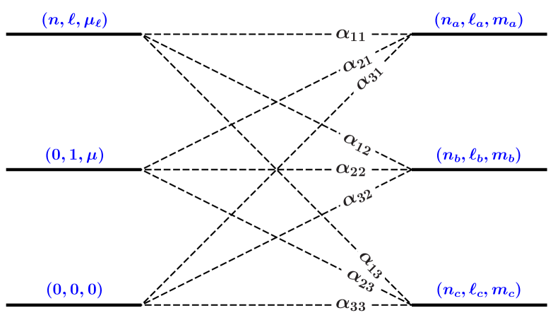
Figure 3: Diagrammatic representation of the spatial parts of formula (37).

The internal lines of diagram (3) are function of the matrix elements $\alpha_{11}$, …, $\alpha_{33}$ of a $3\times 3$ matrix $\alpha$. When we restrict ourselves to the case of equal quark masses, then $\alpha$ is for the first term of (37) given by

$$\left(\begin{array}[]{l}\mbox{\boldmath$r$}_{32}\\[10.0pt] \mbox{\boldmath$r$}_{14}\\[10.0pt] \mbox{\boldmath$r$}_{32,14}\end{array}\right)\;=\;\left(\begin{array}[]{ccc}\frac{1}{2}&\frac{1}{2}&\sqrt{\frac{1}{2}}\\[10.0pt] \frac{1}{2}&\frac{1}{2}&-\sqrt{\frac{1}{2}}\\[10.0pt] \sqrt{\frac{1}{2}}&-\sqrt{\frac{1}{2}}&0\end{array}\right)\left(\begin{array}[]{l}\mbox{\boldmath$r$}_{12}\\[10.0pt] \mbox{\boldmath$r$}_{34}\\[10.0pt] \mbox{\boldmath$r$}_{12,34}\end{array}\right)\;\;\;,$$ (42)

and for the second term by

$$\left(\begin{array}[]{l}\mbox{\boldmath$r$}_{14}\\[10.0pt] \mbox{\boldmath$r$}_{32}\\[10.0pt] \mbox{\boldmath$r$}_{14,32}\end{array}\right)\;=\;\left(\begin{array}[]{ccc}\frac{1}{2}&\frac{1}{2}&-\sqrt{\frac{1}{2}}\\[10.0pt] \frac{1}{2}&\frac{1}{2}&\sqrt{\frac{1}{2}}\\[10.0pt] -\sqrt{\frac{1}{2}}&\sqrt{\frac{1}{2}}&0\end{array}\right)\left(\begin{array}[]{l}\mbox{\boldmath$r$}_{12}\\[10.0pt] \mbox{\boldmath$r$}_{34}\\[10.0pt] \mbox{\boldmath$r$}_{12,34}\end{array}\right)\;\;\;,$$ (43)

We denote the respective results of the diagram of Fig. 3 for the $\alpha$’s defined in Eqs. (42) and (43), respectively by

$$d_{1}\left(n,\ell,\mu_{1};\,\mu;\,n_{a},\ell_{a},m_{a};\,n_{b},\ell_{b},m_{b};\,n_{c},\ell_{c},m_{c}\right)\;\;\;,$$ (44)

and

$$d_{2}\left(n,\ell,\mu_{1};\,\mu;\,n_{a},\ell_{a},m_{a};\,n_{b},\ell_{b},m_{b};\,n_{c},\ell_{c},m_{c}\right)\;\;\;.$$ (45)

With these definitions we obtain for the matrix elements (37):

$${\cal M} = {\cal N}_{1}\left[J,J_{z};\,\ell,s,n;\,(a,b)\right]\sum_{\scriptsize\begin{array}[]{c}m_{a},\mu_{a},m_{b},\mu_{b}\\ m_{c},\mu_{\ell},\mu_{s},\mu_{1},\mu_{2}\\ m_{1},m_{2},m_{3},m_{4}\end{array}}\!\!\!\mbox{$C\begin{array}[]{ccc}\!\!\!J_{c}&\!\!\!\!\ell_{c}&\!\!\!\!J\\ \!\!\!M_{c}&\!\!\!\!m_{c}&\!\!\!\!J_{z}\end{array}$}\,\mbox{$C\begin{array}[]{ccc}\!\!\!J_{a}&\!\!\!\!J_{b}&\!\!\!\!J_{c}\\ \!\!\!M_{a}&\!\!\!\!M_{b}&\!\!\!\!M_{c}\end{array}$}\,$$ (76)

$$C\begin{array}[]{ccc}\!\!\!\ell_{a}&\!\!\!\!s_{a}&\!\!\!\!J_{a}\\ \!\!\!m_{a}&\!\!\!\!\mu_{a}&\!\!\!\!M_{a}\end{array} C\begin{array}[]{ccc}\!\!\!\ell_{b}&\!\!\!\!s_{b}&\!\!\!\!J_{b}\\ \!\!\!m_{b}&\!\!\!\!\mu_{b}&\!\!\!\!M_{b}\end{array} C\begin{array}[]{ccc}\!\!\!\ell&\!\!\!\!s&\!\!\!\!J\\ \!\!\!\mu_{\ell}&\!\!\!\!\mu_{s}&\!\!\!\!J_{z}\end{array} C\begin{array}[]{ccc}\!\!\!\,1&\!\!\!\!1&\!\!\!\!0\\ \!\!\!\mu_{1}&\!\!\!\!\mu_{2}&\!\!\!\!0\end{array} C\begin{array}[]{ccc}\!\!\!\frac{1}{2}&\!\!\!\!\frac{1}{2}&\!\!\!\!s_{a}\\ \!\!\!m_{1}&\!\!\!\!m_{2}&\!\!\!\!\mu_{a}\end{array} C\begin{array}[]{ccc}\!\!\!\frac{1}{2}&\!\!\!\!\frac{1}{2}&\!\!\!\!s_{b}\\ \!\!\!m_{3}&\!\!\!\!m_{4}&\!\!\!\!\mu_{b}\end{array}$$

$$\left\{d_{1}\left(n,\ell,\mu_{1};\,\mu;\,n_{a},\ell_{a},m_{a};\,n_{b},\ell_{b},m_{b};\,n_{c},\ell_{c},m_{c}\right)\,\mbox{$C\begin{array}[]{ccc}\!\!\!\frac{1}{2}&\!\!\!\!\frac{1}{2}&\!\!\!\!s\\ \!\!\!m_{3}&\!\!\!\!m_{2}&\!\!\!\!\mu_{s}\end{array}$}\,\mbox{$C\begin{array}[]{ccc}\!\!\!\frac{1}{2}&\!\!\!\!\frac{1}{2}&\!\!\!\!1\\ \!\!\!m_{1}&\!\!\!\!m_{4}&\!\!\!\!\mu_{2}\end{array}$}\,\delta_{a^{\prime}b^{\prime}}\,\delta_{d^{\prime}b}\,\delta_{c^{\prime}a}\;+\right.$$

$$\left.+\;d_{2}\left(n,\ell,\mu_{1};\,\mu;\,n_{a},\ell_{a},m_{a};\,n_{b},\ell_{b},m_{b};\,n_{c},\ell_{c},m_{c}\right)\,\mbox{$C\begin{array}[]{ccc}\!\!\!\frac{1}{2}&\!\!\!\!\frac{1}{2}&\!\!\!\!s\\ \!\!\!m_{1}&\!\!\!\!m_{4}&\!\!\!\!\mu_{s}\end{array}$}\,\mbox{$C\begin{array}[]{ccc}\!\!\!\frac{1}{2}&\!\!\!\!\frac{1}{2}&\!\!\!\!1\\ \!\!\!m_{3}&\!\!\!\!m_{2}&\!\!\!\!\mu_{2}\end{array}$}\delta_{a^{\prime}a}\,\delta_{d^{\prime}c^{\prime}}\,\delta_{b^{\prime}b}\right\}\;.$$

In Sect. 2 we smuggled two assumptions into the procedure, which had to do with the excitations of the ${}^{3}P_{0}$-pair. This resulted in the four zero’s in diagram (3). The generalization to other quantum numbers is straightforward but will not be treated here.

5 Results and comparison with experiment

In this section we study the results of expression (76) for some quark-antiquark systems. First we introduce the nomenclature which has been used here for mesons. In Table 1, we give the precise meaning of the symbols which we use in Table 2.

meson	$q\bar{q}$	$n{{}^{2S+1}L}_{J}$	$J^{PC}$
pseudoscalars	ground state	1$\,{{}^{1}S}_{0}$	$0^{-+}$
	first radial excitation	2$\,{{}^{1}S}_{0}$	${0^{\prime}}^{-+}$
vectors	ground state	1$\,{{}^{3}S}_{1}$	$1^{--}$
	first radial excitation	2$\,{{}^{3}S}_{1}$	${1^{\prime}}^{--}$
	second angular excitation	1$\,{{}^{3}D}_{1}$	${1^{\prime\prime}}^{--}$
scalars	ground state	1$\,{{}^{3}P}_{0}$	$0^{++}$
axial vectors	ground state ($S=1$)	1$\,{{}^{3}P}_{1}$	$1^{++}$
	ground state ($S=0$)	1$\,{{}^{1}P}_{1}$	$1^{+-}$

Table 1: Nomenclature of quark-antiquark systems. The columns contain respectively, the most current denomination for mesons, the assumed $q\bar{q}$ state, the $q\bar{q}$-quantum numbers ($n$ is the assumed radial quantum-number, $S$ represents the total spin, $L$ the orbital and $J$ total angular momentum), and the more common quantum numbers ($P$ stands for parity and $C$ for charge conjugation; excitations are indicated by accents).

In Table 2, all (i.e. within the above specified assumptions) possible decay channels for the lowest radial and angular excitations of pseudoscalar, vector and scalar mesons are given.

	$0^{-+}$	$1^{--}$	$0^{++}$
$(0^{-+}\,,0^{-+}\,)$		$-\frac{1}{24}\left(1{{}^{1}P}\right)$	$\frac{1}{24}\left(2{{}^{1}S}\right)$
$(0^{-+}\,,{0^{\prime}}^{-+}\,)$			$\frac{1}{48}\left(1{{}^{1}S}\right)$
$(0^{-+}\,,1^{--}\,)$	$-\frac{1}{4}\left(1{{}^{3}P}\right)$	$\frac{1}{6}\left(1{{}^{3}P}\right)$
$(0^{-+}\,,0^{++}\,)$	$\frac{1}{8}\left(1{{}^{1}S}\right)$
$(0^{-+}\,,1^{++}\,)$		$-\frac{1}{12}\left(1{{}^{3}S}\right)$	$\frac{1}{6}\left(1{{}^{3}P}\right)$
$(0^{-+}\,,1^{+-}\,)$		$\frac{1}{24}\left(1{{}^{3}S}\right)$
$(1^{--}\,,1^{--}\,)$	$\frac{1}{4}\left(1{{}^{3}P}\right)$	$-\frac{1}{72}\left(1{{}^{1}P}\right)$	$\frac{1}{72}\left(2{{}^{1}S}\right)$
$(1^{--}\,,1^{--}\,)$		$-\frac{5}{18}\left(1{{}^{5}P}\right)$	$\frac{5}{18}\left(1{{}^{5}D}\right)$
$(1^{--}\,,{1^{\prime}}^{--}\,)$			$\frac{1}{144}\left(1{{}^{1}S}\right)$
$(1^{--}\,,{1^{\prime\prime}}^{--}\,)$			$\frac{5}{36}\left(1{{}^{1}S}\right)$
$(1^{--}\,,1^{++}\,)$	$-\frac{1}{4}\left(1{{}^{1}S}\right)$	$\frac{1}{6}\left(1{{}^{3}S}\right)$
$(1^{--}\,,1^{+-}\,)$	$\frac{1}{8}\left(1{{}^{1}S}\right)$	$-\frac{1}{12}\left(1{{}^{3}S}\right)$	$\frac{1}{6}\left(1{{}^{3}P}\right)$
$(0^{++}\,,0^{++}\,)$			$\frac{1}{16}\left(1{{}^{1}S}\right)$
$(0^{++}\,,1^{--}\,)$		$\frac{1}{8}\left(1{{}^{3}S}\right)$
$(1^{++}\,,1^{++}\,)$			$\frac{1}{12}\left(1{{}^{1}S}\right)$
$(1^{+-}\,,1^{+-}\,)$			$\frac{1}{48}\left(1{{}^{1}S}\right)$

Table 2: Three-meson vertices $\left|\mbox{$\left\langle MM\left|V\right|M\right\rangle$}\right|^{2}$. The signs in front of the matrixelements are explained in the text. The orbital quantum numbers of the meson-meson system are given between brackets, in the spectroscopic notation $n{{}^{2S+1}L}$, where $n$ is radial quantum number, $S$ the spin and $L$ the angular momentum.

Note that the figures in each column of Table 2 add up to 1. This expresses the fact that each wave function (38) can be completely decomposed into the basis (39), because both sets are solutions of the same Hamiltonian.

The signs which are given in Table 2 are the results of the ratios of the terms stemming from $P^{13}$ and the terms stemming from $P^{24}$ in formula (37). These signs are essential for conservation of $G$-parity, which can easily been seen once the $SU(3)$-flavor content is taken into account.

We are now prepared to test the results of Table 2 to the available data.

In general the width of a decaying particle is given (see e.g. Ref. [11]) by

$$\Gamma\;=\;\frac{\textstyle k}{\textstyle 4m^{2}}\,\int\,d\cos(\vartheta)\,\left|\frac{\textstyle T\left(m^{2},\cos(\vartheta)\right)}{\textstyle\sqrt{4\pi}}\right|^{2}\;\;\;.$$ (77)

The matrix element $T$ in Eq. (77) includes the calculation of the overlap between the free meson wave function and the harmonic oscillator basis, which we have chosen. In fact we should do

$$\mbox{$\left\langle MM\left|V\right|M\right\rangle$}\;=\;\sum_{n,n^{\prime}}\,\left\langle MM\left|n^{\prime}\right.\right\rangle\mbox{$\left\langle n^{\prime}\left|V\right|n\right\rangle$}\left\langle n\left|M\right.\right\rangle\;\;\;,$$ (78)

where $\left|M\right\rangle$ is a specific initial state of the $q\bar{q}$ mesonic system and $\left|MM\right\rangle$ represents the final state of the two decay products. But, since decay widths can be better calculated from the solutions of the multichannel Schrödinger equation involving the transition potential (this is done by us in a different program [9, 10]), we will not be too rigorous in demonstrating that the matrix elements (77) make sense. So we assume that $\left\langle n\left|M\right.\right\rangle$ is only nonzero for one value of $n$, and that then also the corresponding $\left\langle MM\left|n^{\prime}\right.\right\rangle$ is the only nonzero term. The overlap of the plane waves for the two meson system and a harmonic oscillator contains a momentum dependence of the form

$$T\;\propto\;k^{\ell}\;\;\;.$$ (79)

where $\ell$ is the relative orbital angular momentum of the decay products. Relation (79), together with the phase space factor, gives

$$\Gamma\;\propto\;k^{2\ell+1}\;\;\;.$$ (80)

So, we arrive at

$$\Gamma\;\propto\;k^{2\ell+1}\,\left|\mbox{$\left\langle n^{\prime}\left|V\right|n\right\rangle$}\right|^{2}\;\;\;,$$ (81)

where $n$ represents the radial quantum number of the decaying meson. A more precise form of formula (81) is given by the imaginary part of the second order perturbation contribution to the energy within the model [9, 10], as is given in [12, 13]. We will, however, take (81) as sufficiently accurate for our purpose here.

As examples we study the decay widths of $\epsilon$(1300) (nowadays $f_{0}$(1370)), $a_{2}$(1320), and $K^{\ast}_{0}$(1430), which particles have enough two particle decay modes, to make a comparison of relation (81) to the available data possible. The results are given in Table 3.

processes	Eq. (81)	PDG80	PDG04
$\frac{\textstyle\epsilon\to K\bar{K}}{\textstyle\epsilon\to\pi\pi}$	0.22	0.11	0.12$\pm$0.06 - 0.91$\pm$0.20
$\frac{\textstyle a_{2}\to\eta\pi}{\textstyle a_{2}\to\rho\pi}$	0.37	0.20 - 0.25	0.213$\pm$0.020
$\frac{\textstyle K^{\ast}_{0}\to K\pi}{\textstyle K^{\ast}_{0}\to K^{\ast}\pi}$	2.28	1.6 - 2.1	2.02$\pm$0.14
$\frac{\textstyle K^{\ast}_{0}\to K\pi}{\textstyle K^{\ast}_{0}\to K\rho}$	7.76	4.3 - 6.1	6.7$\pm$1.1
$\frac{\textstyle K^{\ast}_{0}\to K\eta}{\textstyle K^{\ast}_{0}\to K\omega}$	2.93	0 - 3.7	-

Table 3: Some branching ratios of $\epsilon$(1300) (nowadays $f_{0}$(1370)), $a_{2}$(1320), and $K^{\ast}_{0}$(1430). Results of expression (81) compared to experiment: PDG80, C. Bricman et al., Rev. Mod. Phys. 52, 1 (1980), and PDG04, S. Eidelman et al., Phys. Lett. B592, 1 (2004)

6 The transition potential

Inspired by the reasonable results of the comparison of our handwaving calculations with the data, we will derive in this section a transition potential for a coupled channel Schrödinger equation as described in [9, 10]. In [5] we have shown how we might arrive at a local approximation of the potential for transitions from a quark-antiquark channel to a meson-meson channel. The outline given there will be made more precise in this section.

The potential is given by

$$\mbox{$\left\langle MM,x\left|V\right|M,x\right\rangle$}\;=\;\sum_{n,n^{\prime}}\,\left\langle MM,x\left|n^{\prime}\right.\right\rangle\mbox{$\left\langle n^{\prime}\left|V\right|n\right\rangle$}\left\langle n\left|M,x\right.\right\rangle\;\;\;,$$ (82)

The wave functions are in lowest order assumed to be given by

$$\left\langle n\left|M,x\right.\right\rangle\;=\;\phi_{\,n,\ell,\mu_{\ell}}\left(\sqrt{\frac{1}{2}m\omega}\,x\right)\;\;\;,$$ (83)

where ($\ell$, $\mu_{\ell}$) are the orbital quantum numbers of the $q\bar{q}$ mesonic system, where $m$ is the quarkmass and where $\omega$ is the universal oscillator frequency, and by

$$\left\langle n^{\prime}\left|MM,x\right.\right\rangle\;=\;\phi_{\,n^{\prime},\ell^{\prime},{\mu^{\prime}}_{\ell}}\left(\sqrt{m\omega}\,x\right)\;\;\;,$$ (84)

where ($\ell^{\prime}$, ${\mu^{\prime}}_{\ell}$) are the orbital quantum numbers of the two meson system.

The matrix elements $\left\langle n^{\prime}\left|V\right|n\right\rangle$ are those given in [5]. For the lowest lying $q\bar{q}$ systems $n^{\prime}$ is linearly related to $n$.

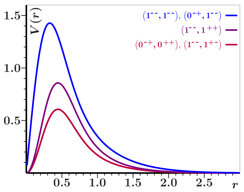
Figure 4: Transition potentials for the decay of pseudoscalar mesons ($r$ and $V(r)$ are dimensionless). The curves are determined with expression (82) for the five three-meson vertices of Table (2).
The upper curve (blue) corresponds to the pseudoscalar vertices with (vector, vector) and (pseudoscalar, vector) the middle curve (violet) to the pseudoscalar vertex with (vector, positive-$C$-parity axial vector), the lower curve (red) to the pseudoscalar vertices with (pseudoscalar, scalar) and (vector, negative-$C$-parity axial vector).

In Fig. 4 we present the results of Eq. (82) for the decay processes of pseudoscalar particles. Although in Table 2 five different types of decay channels for a pseudoscalar meson are shown, we find that the spatial behavior for two pairs is exactly the same. We also observe from Fig. 4 that the decay processes $P\to PV$ and $P\to VV$ are dominant. This result is important because it justifies the procedure of [9, 10]. There we have limited us to these channels. For doing so we now have two arguments: the thresholds are low, the couplings are largest. We also find that the form of the here calculated transition potential is in agreement with the one from [10]. However, in [10] the position of the peak is a parameter which can be fitted to the data, whereas here it is a result of our procedure.

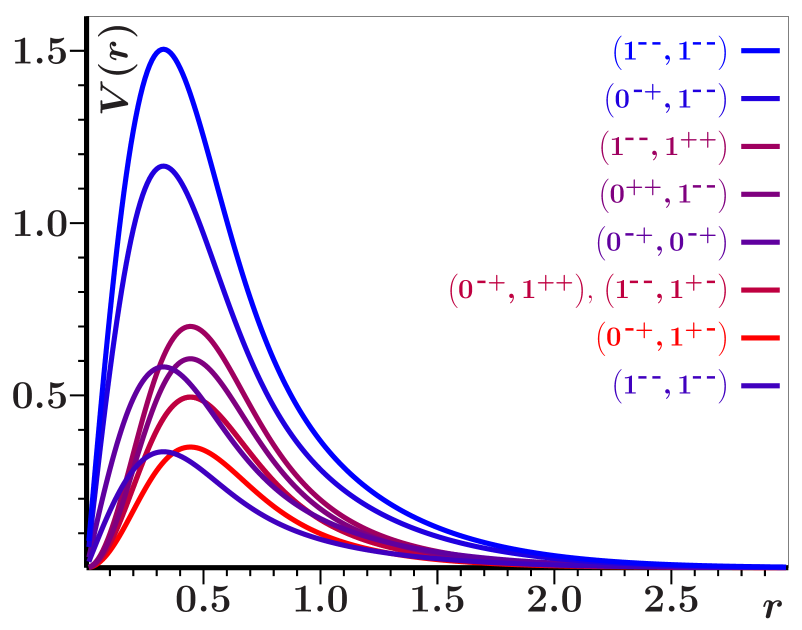
Figure 5: Transition potentials for the decay of vector mesons ($r$ and $V(r)$ are dimensionless). The curves are determined with expression (82) for the nine three-meson vertices of Table (2).
The curves, from the curve with the highest maximum to the curve with the lowest maximum, represent the vector vertices with respectively (vector, vector in $P$ wave, total spin $S=2$), (pseudoscalar, vector), (vector, positive-$C$-parity axial vector), (scalar, vector), (pseudoscalar, pseudoscalar), (pseudoscalar, positive-$C$-parity axial vector) and (vector, negative-$C$-parity axial vector), (pseudoscalar, negative-$C$-parity axial vector), (vector, vector in $P$ wave, total spin $S=0$).

In Figs. 5 and 6 are depicted similar results for the vector and the scalar mesons respectively. Is it reasonable in the case of pseudoscalar mesons to select two dominant decay modes, in the case of vector mesons the situation is less comfortable (see Fig. 5) and becomes even hopeless in the case of scalar mesons (Fig. 6).

So, in the next stage of the program of the multi-channel model of [9, 10] all possible decay channels should be taken into account in order to decide afterwards which of them are important for the description of a specific hadron. The here presented method can supply us with the precise form of the transition potentials. Finally we must notice that the potentials of the Figs. 4, 5 and 6, exhibit a peaked structure. In [12] it is argued that such types of potentials can very easily explain the radial hadron spectra, especially the large level splittings between the ground states and the first radial excitations with respect to the other mass differences.

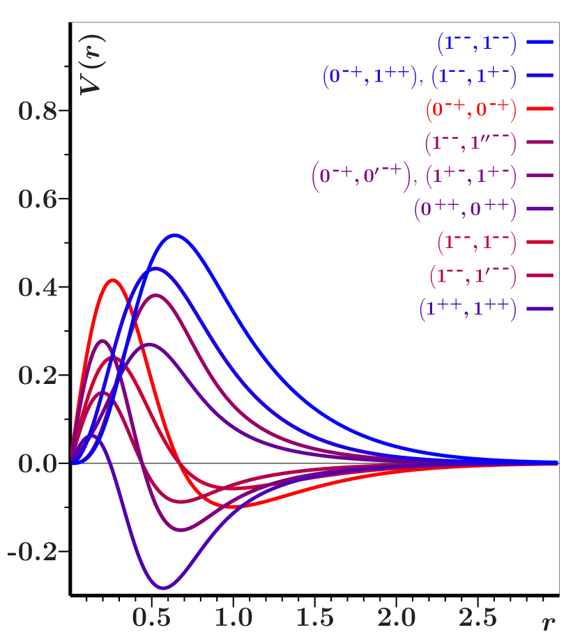
Figure 6: Transition potentials for the decay of scalar mesons ($r$ and $V(r)$ are dimensionless). The curves are determined with expression (82) for the eleven three-meson vertices of Table (2).
The curves, from the curve with the highest maximum to the curve with the lowest maximum, represent the scalar vertices with respectively (vector, vector in $D$ wave, total spin $S=2$), (pseudoscalar, positive-$C$-parity axial vector) and (vector, negative-$C$-parity axial vector), (pseudoscalar, pseudoscalar), (vector, vector (angular excitation)), (pseudoscalar, pseudoscalar (radial excitation)) and (negative-$C$-parity axial vector, negative-$C$-parity axial vector), (scalar, scalar), (vector, vector in $S$ wave, total spin $S=0$), (vector, vector (radial excitation)), (positive-$C$-parity axial vector, positive-$C$-parity axial vector).

Conclusions

We have shown here that the method which was roughly outlined in [5], can indeed be used for the construction of transition potentials to be used in coupled channel models [9, 10] for mesons (and baryons). The procedure is still not unambiguous, but, for a first inspection of the results, very suitable. The next refinement could be, to take different quark masses in the matrix elements (76). This leads to different transition potentials for decay due to the creation of up and down quark pairs as for decay due to the creation of strange quark pairs. Another possibility is, to repeat the whole procedure for the $SO(3,2)$ wave functions of [14], which are probably more realistic than harmonic oscillator wave functions.

Acknowledgments

I thank Prof. Dr. C. Dullemond for the formulation of the program to be followed and Dr. T. A. Rijken for many useful conversations.

Part of this work was included in the research program of the Stichting voor Fundamenteel Onderzoek der Materie (F.O.M.) with financial support from the Nederlandse Organizatie voor ZuiverWetenschappelijk Onderzoek (Z.W.O.).

References

- [1] E. Eichten, K. Gottfried, T. Kinoshita, K. D. Lane and T. M. Yan, Charmonium: 1. The Model, Phys. Rev. D 17, 3090 (1978) [Erratum-ibid. D 21, 313 (1980)]. E. Eichten, K. Gottfried, T. Kinoshita, K. D. Lane and T. M. Yan, Charmonium: Comparison With Experiment, Phys. Rev. D 21 (1980) 203.
- [2] S. Jacobs, K. J. Miller and M. G. Olsson Quarkonium bound states and coupling to hadrons, Phys. Rev. Lett. 50, 1181 (1983).
- [3] K. Heikkilä, S. Ono and N. A. Törnqvist, Heavy and quarkonium states and unitarity effects, Phys. Rev. D 29, 110 (1984) [Erratum-ibid. D 29, 2136 (1984)].
- [4] C. Dullemond, T. A. Rijken, E. van Beveren and G. Rupp, On The Influence Of Hadronic Decay On The Properties Of Hadrons, in proceedings of VIth Warsaw Symposium on Elementary Particle Physics, Kazimierz, Poland, 30 May - 3 Jun 1983, pp 257-262.
- [5] E. van Beveren, Recoupling matrix elements and decay, Z. Phys. C 17, 135 (1983) [arXiv:hep-ph/0602248].
- [6] L. Micu, Decay rates of meson resonances in a quark model, Nucl. Phys. B 10, 521 (1969). R. D. Carlitz and M. Kislinger, Regge amplitude arising from vertices, Phys. Rev. D 2 (1970) 336.
- [7] A. Le Yaouanc, L. Oliver, O. Pène and J. C. Raynal, Naive quark-pair-creation model of strong-interaction vertices, Phys. Rev. D 8 (1973) 2223. A. Le Yaouanc, L. Oliver, O. Pène and J. C. Raynal, Naive quark-pair-creation model and baryon decays, Phys. Rev. D 9 (1974) 1415.
- [8] M. Chaichian and R. Kögerler, Coupling constants and the nonrelativistic quark model with charmonium potential, Annals Phys. 124, 61 (1980).
- [9] E. van Beveren, C. Dullemond, and G. Rupp, Spectra and strong decays of and states, Phys. Rev. D 21, 772 (1980) [Erratum-ibid. D 22, 787 (1980)].
- [10] E. van Beveren, G. Rupp, T. A. Rijken, and C. Dullemond, Radial spectra and hadronic decay widths of light and heavy mesons, Phys. Rev. D 27, 1527 (1983).
- [11] H. Pilkuhn, The interaction of hadrons, Amsterdam: North Holland publishing company, 1967
- [12] E. van Beveren, C. Dullemond and T. A. Rijken, On the influence of hadronic decay on the properties of hadrons, Z. Phys. C 19, 275 (1983).
- [13] C. Dullemond and E. van Beveren, Confining potentials and Regge poles, Ann. Phys. 105, 318 (1977).
- [14] E. van Beveren, T. A. Rijken and C. Dullemond, Quarks in an anti-De Sitter geometry, Nijmegen-report THEF-NYM-79-11 (1979).