Revisiting $\gamma\gamma\to\pi^{+}\pi^{-}$ at low energies

Abstract

We complete the recalculation of the available two-loop expressions for the reaction $\gamma\gamma\to\pi\pi$ in the framework of chiral perturbation theory. Here, we present the results for charged pions. The cross section and the values of the dipole polarizabilities agree very well with the earlier calculation, provided the same set of low-energy constants (LECs) is used. With updated values for the LECs at order $p^{4}$, we find for the dipole polarizabilities $(\alpha_{1}-\beta_{1})_{\pi^{\pm}}=(5.7\pm 1.0)\times 10^{-4}\,{\rm fm}^{3}$, which is in conflict with the experimental result recently reported by the MAMI Collaboration.

PACS: 11.30.Rd; 12.38.Aw; 12.39.Fe; 13.60.Fz

, ,

1 Introduction

We evaluate the amplitude for $\gamma\gamma\rightarrow\pi^{+}\pi^{-}$ in the framework of chiral perturbation theory (ChPT  ) [1, 2, 3] at two-loop order, and compare the result with the only previous calculation performed at this accuracy [4]. We employ the calculational techniques outlined in our previous work [5], which allow us to provide a rather compact and easy to use integral representation for the full amplitude. We find that the cross section for the reaction $\gamma\gamma\rightarrow\pi^{+}\pi^{-}$ and the dipole polarizabilities agree very well with the results reported in Ref. [4], provided that the same set of LECs is used. With updated LECs at order $p^{4}$ [6, 7], we find for the dipole polarizabilities the value

$$(\alpha_{1}-\beta_{1})_{\pi^{\pm}}=(5.7\pm 1.0)\times 10^{-4}\,{\rm fm}^{3}\,.$$ (1.1)

The MAMI Collaboration [8] has recently reported the experimental result

$$(\alpha_{1}-\beta_{1})_{\pi^{\pm}}=(11.6\pm 1.5_{\rm stat}\pm 3.0_{\rm syst}\pm 0.5_{\rm mod})\times 10^{-4}\,{\rm fm}^{3}\,.$$ (1.2)

The index “mod” denotes the uncertainty generated by the theoretical models used to analyse the data. The ChPT calculation is in conflict with this prediction, see also [9] for a recent discussion.

There are good reasons to believe that the chiral prediction Eq. (1.1) is rather stable against contributions from still higher orders in the chiral expansion. The main point is that the Born-term subtracted amplitude - in terms of which the polarizabilities are defined - is regular at the Compton threshold. Therefore, the influence of chiral logarithms is suppressed as compared to the amplitude at, say, the threshold for $\pi\pi$ production, where the amplitude generates a branch point. Further, we have analysed the potential influence of resonance exchange and could not identify any significant contribution from nearby resonances to the combination $(\alpha_{1}-\beta_{1})_{\pi^{\pm}}$. We conclude that the low-energy constants at order $p^{6}$ are expected to play a negligible effect here. In view of these observations, the discrepancy between the chiral prediction and the recent MAMI data cannot be explained.

The article is organized as follows. In Section 2 we spell out the kinematics of the process $\gamma\gamma\rightarrow\pi^{+}\pi^{-}$. To make the article selfcontained, we summarize in Section 3 the necessary ingredients of the effective Lagrangian framework. Here, we also fix the LECs to be used in numerical calculations. In Section 4, we display the Feynman diagrams and discuss shortly their evaluation. Section 5 contains a concise representation of the two Lorentz invariant amplitudes that describe the scattering matrix element. Section 6 contains explicit expressions for the dipole and quadrupole polarizabilities valid at next-to-next-to-leading order in the chiral expansion, together with a detailed numerical analysis and a comparison with the recent MAMI data [8], and with an evaluation from data on $\gamma\gamma\rightarrow\pi^{+}\pi^{-}$  [10]. The summary and an outlook are given in Section 7. A detailed comparison with the earlier calculation [4] is provided in Appendix A, and several technical aspects of the calculation are relegated to additional Appendices B-D.

2 Kinematics

The amplitude describing the process $\gamma\gamma\rightarrow\pi^{+}\pi^{-}$ may be extracted from the matrix element

$$\;\langle\;\pi^{+}(p_{1})\pi^{-}(p_{2})\;{\rm out}\;|\;\gamma(q_{1})\gamma(q_{2})\;{\rm in}\;\rangle\;=i(2\pi)^{4}\delta^{4}(P_{f}-P_{i})\;T^{\gamma\gamma\rightarrow\pi^{+}\pi^{-}},$$ (2.1)

where

$$T^{\gamma\gamma\rightarrow\pi^{+}\pi^{-}} = e^{2}\epsilon_{1}^{\mu}\epsilon_{2}^{\nu}\,W_{\mu\nu}^{\gamma\gamma\rightarrow\pi^{+}\pi^{-}}\;,$$

$$W_{\mu\nu}^{\gamma\gamma\rightarrow\pi^{+}\pi^{-}} = i\int\!dx\,e^{-i(q_{1}x+q_{2}y)}\;\langle\;\pi^{+}(p_{1})\pi^{-}(p_{2})\;{\rm out}\;|\;Tj_{\mu}(x)j_{\nu}(y)\;|\;0\;\rangle\;.$$ (2.2)

Here $j^{\mu}$ denotes the electromagnetic current and $\alpha=e^{2}/4\pi\simeq 1/137$ is the electromagnetic coupling. It is convenient to change the pion coordinates according to $(\pi^{\pm},\pi^{0})\rightarrow(\pi^{1},\pi^{2},\pi^{3})$ and instead of $\pi^{+}\pi^{-}$–production, we consider in the following the process $\gamma\gamma\rightarrow\pi^{1}\pi^{1}$, with

$$W_{\mu\nu}^{\gamma\gamma\rightarrow\pi^{+}\pi^{-}}=-W_{\mu\nu}^{\gamma\gamma\rightarrow\pi^{1}\pi^{1}}\doteq-V_{\mu\nu}\;,$$ (2.3)

where the relative minus sign stems from the Condon–Shortly phase convention. [We use the same sign convention as Ref. [4].] The decomposition of the correlator $V_{\mu\nu}$ into Lorentz invariant amplitudes reads

$$V_{\mu\nu} = A(s,t,u)T_{1\,\mu\nu}+B(s,t,u)T_{2\,\mu\nu}+C(s,t,u)T_{3\,\mu\nu}+D(s,t,u)T_{4\,\mu\nu}\,,$$

$$T_{1\,\mu\nu} = \frac{1}{2}\,s\,g_{\mu\nu}-q_{1\nu}q_{2\mu}\,,$$

$$T_{2\,\mu\nu} = 2\,s\,\Delta_{\mu}\Delta_{\nu}-\nu^{2}\,g_{\mu\nu}-2\,\nu\,(q_{1\,\nu}\Delta_{\mu}-q_{2\,\mu}\Delta_{\nu})\,,$$

$$T_{3\,\mu\nu} = q_{1\,\mu}q_{2\,\nu}\,,$$

$$T_{4\,\mu\nu} = s\,(q_{1\,\mu}\Delta_{\nu}-q_{2\,\nu}\Delta_{\mu})-\nu\,(q_{1\,\mu}q_{1\,\nu}+q_{2\,\mu}q_{2\,\nu})\,,$$

$$\Delta_{\mu} = (p_{1}-p_{2})_{\mu}\,,$$ (2.4)

where

$$s = (q_{1}+q_{2})^{2},\;\;\;t=(p_{1}-q_{1})^{2},\;\;\;u=(p_{2}-q_{1})^{2},\;\;\;\nu=t-u\,$$ (2.5)

are the standard Mandelstam variables. The tensor $V_{\mu\nu}$ satisfies the Ward identities

$$q^{\mu}_{1}\,V_{\mu\nu}=q^{\nu}_{2}\,V_{\mu\nu}=0.$$ (2.6)

The amplitudes $A$ and $B$ are analytic functions of the variables $s,t$ and $u$, symmetric under crossing $(t,u)\rightarrow(u,t)$. The amplitudes $C$ and $D$ do not contribute to the process considered here, because $\epsilon_{i}\cdot q_{i}=0$.

It is useful to introduce in addition the helicity amplitudes

$${\bar{H}}_{++} = A+2\,(4\,M^{2}_{\pi}-s)\,B\,,\qquad{\bar{H}}_{+-}=\frac{8\,(M_{\pi}^{4}-t\,u)}{s}\,B.$$ (2.7)

The helicity components ${\bar{H}}_{++}$ and ${\bar{H}}_{+-}$ correspond to photon helicity differences $\lambda=0,2$, respectively. With our normalization of states $\langle\mathbf{p_{1}}|\mathbf{p_{2}}\rangle=2\,(2\pi)^{3}\,p_{1}^{0}\,\delta^{(3)}(\mathbf{p_{1}}-\mathbf{p_{2}})$, the differential cross section for unpolarized photons in the centre-of-mass system is

$${\frac{d\sigma}{d\Omega}}^{\gamma\gamma\rightarrow\pi^{+}\pi^{-}} = \frac{\alpha^{2}\,s}{32}\beta(s)\,H(s,t)\,,\hskip 28.45274ptH(s,t)=|{\bar{H}}_{++}|^{2}+|{\bar{H}}_{+-}|^{2}\,,$$ (2.8)

with $\beta(s)=\sqrt{1-4\,M^{2}_{\pi}/s}$. The relation between the helicity amplitudes $M_{+\pm}$ in Ref. [10] and the amplitudes used here is

$$M_{++}(s,t)=2\pi\alpha{\bar{H}}_{++}(s,t)\,,\qquad M_{+-}(s,t)=16\pi\alpha B(s,t)\,.$$ (2.9)

In the centre-of-mass system, $\vec{q}_{1}+\vec{q}_{2}=0$, one has $\vec{q}_{1}\cdot\vec{p}_{1}=|\vec{q}_{1}||\vec{p}_{1}|\cos\theta$, where $\theta$ is the scattering angle. Then the Mandelstam variables are given by

$$s=4\,|\vec{q}|^{2},\qquad t=M^{2}_{\pi}-(s/2)\left(1-\beta(s)\cos\theta\right).$$ (2.10)

For comparison with experimental data, it is convenient to present also the total cross section for the case having $|\cos\theta|$ less than some fixed value $Z$,

$$\sigma(s;|\cos\theta|<Z)=\frac{\alpha^{2}\pi}{8}\int\limits_{t_{-}}^{t_{+}}dtH(s,t)$$ (2.11)

with $t_{\pm}=M_{\pi}^{2}-(s/2)\;(1\mp\beta(s)Z)$.

3 The effective Lagrangian and its low-energy constants

The effective Lagrangian consists of a string of terms. Here, we consider QCD with two flavours, in the isospin symmetry limit $m_{u}=m_{d}=\hat{m}$. At next-to-next-to-leading order (NNLO), one has [2]

$${\mathcal{L}}_{\rm eff}={\mathcal{L}}_{2}+{\mathcal{L}}_{4}+{\mathcal{L}}_{6}\,.$$ (3.1)

The subscripts refer to the chiral order. The expression for ${\mathcal{L}}_{2}$ is

$${\mathcal{L}}_{\,2} = \frac{F^{2}}{4}\langle D_{\mu}U\,D^{\mu}U^{\dagger}+M^{2}(U+U^{\dagger})\rangle\,,$$

$$D_{\mu}U = \partial_{\mu}U-i(QU-UQ)A_{\mu}\,,\,\ Q=\frac{e}{2}{\rm diag}(1,-1)\,,$$ (3.2)

where $e$ is the electric charge, and $A_{\mu}$ denotes the electromagnetic field. The quantity $F$ denotes the pion decay constant in the chiral limit, and $M^{2}$ is the leading term in the quark mass expansion of the pion (mass)², $M_{\pi}^{2}=M^{2}(1+O(\hat{m}))$. Further, the brackets $\langle\ldots\rangle$ denote a trace in flavour space. In Eq. (3), we have retained only the terms relevant for the present application, i.e., we have dropped additional external fields. We choose the unitary $2\times 2$ matrix $U$ in the form

$$U = \sigma+i\,\pi/F\,,\hskip 8.5359pt\sigma^{2}+\frac{\pi^{2}}{F^{2}}={\mathbf{1}}_{2\times 2}\,,\hskip 8.5359pt\pi=\left(\mbox{$\begin{array}[]{cc}\pi^{0}&\sqrt{2}\,\pi^{+}\\ \sqrt{2}\,\pi^{-}&-\pi^{0}\end{array}$}\right)\;.$$ (3.5)

The Lagrangian at NLO has the structure [2]

$${\mathcal{L}}_{4}=\sum_{i=1}^{7}l_{i}K_{i}+\sum_{i=1}^{3}h_{i}\bar{K}_{i}=\frac{l_{1}}{4}\langle D_{\mu}U\,D^{\mu}U^{\dagger}\rangle^{2}+\cdots\,,$$ (3.6)

where $l_{i},h_{i}$ denote low-energy couplings, not fixed by chiral symmetry. At NNLO, one has [11, 12, 13]

$${\mathcal{L}}_{6}=\sum_{i=1}^{57}c_{i}P_{i}\,.$$ (3.7)

For the explicit expressions of the polynomials $K_{i},\bar{K}_{i}$ and $P_{i}$, we refer the reader to Refs. [2, 11, 12, 13]. The vertices relevant for $\gamma\gamma\rightarrow\pi^{+}\pi^{-}$ involve $l_{1},\ldots,l_{6}$ from ${\mathcal{L}}_{4}$ and several $c_{i}$’s from ${\mathcal{L}}_{6}$, see below.

The couplings $l_{i}$ and $c_{i}$ absorb the divergences at order $p^{4}$ and $p^{6}$, respectively,

$$l_{i} = (\mu\,c)^{d-4}\left\{l_{i}^{r}(\mu,d)+\gamma_{i}\,\Lambda\right\}\,,$$

$$c_{i} = \frac{(\mu\,c)^{2(d-4)}}{F^{2}}\left\{c_{i}^{r}(\mu,d)-\gamma_{i}^{(2)}\,\Lambda^{2}-(\gamma_{i}^{(1)}+\gamma_{i}^{(L)}(\mu,d))\,\Lambda\right\}\,,$$

$$\Lambda = \frac{1}{16\,\pi^{2}(d-4)}\,,\,\ln c=-\frac{1}{2}\left\{\ln 4\pi+\Gamma^{\prime}(1)+1\right\}\,.$$ (3.8)

The physical couplings are $l_{i}^{r}(\mu,4)$ and $c_{i}^{r}(\mu,4)$, denoted by $l_{i}^{r},c_{i}^{r}$ in the following. The coefficients $\gamma_{i}$ are given in [2], and $\gamma_{i}^{(1,2,L)}$ are tabulated in [12]. In order to compare the present calculation with the result of [4], we shall use the scale independent quantities $\bar{l}_{i}$ introduced in [2],

$$l_{i}^{r} = \frac{\gamma_{i}}{32\pi^{2}}\,({\bar{l}}_{i}+l)\,,$$ (3.9)

where the chiral logarithm is $l=\ln(M^{2}_{\pi}/\mu^{2})$. We shall use [6]

$$\bar{l}_{1}=-0.4\pm 0.6\,,\,\,\bar{l}_{2}=4.3\pm 0.1\,,\,\,\bar{l}_{3}=2.9\pm 2.4\,,\,\,\bar{l}_{4}=4.4\pm 0.2\,,$$ (3.10)

and

$$\bar{l}_{\Delta}\doteq\bar{l}_{6}-\bar{l}_{5}=3.0\pm 0.3$$ (3.11)

obtained from radiative pion decay to two loop accuracy [7, 14].

The constants $c_{i}^{r}$ occur in the combinations

$$a_{1}^{r} = -4096\pi^{4}\left(6\,c_{6}^{r}+c_{29}^{r}-c_{30}^{r}-3\,c_{34}^{r}+c_{35}^{r}+2\,c_{46}^{r}-4\,c_{47}^{r}+c_{50}^{r}\right)\,,$$

$$a_{2}^{r} = 256\pi^{4}\left(8\,c_{29}^{r}-8\,c_{30}^{r}+c_{31}^{r}+c_{32}^{r}-2\,c_{33}^{r}+4\,c_{44}^{r}+8\,c_{50}^{r}-4\,c_{51}^{r}\right)\,,$$

$$b^{r} = -128\pi^{4}\left(c_{31}^{r}+c_{32}^{r}-2\,c_{33}^{r}-4\,c_{44}^{r}\right)\,.$$

Their values have been estimated by resonance exchange e.g. in Ref. [4]. We have repeated that analysis. Taking into account $\rho,a_{1}$ and $b_{1}$ exchange which contribute with a definite sign, we obtain

$$\Big{(}a_{1}^{r},a_{2}^{r},b^{r}\Big{)}=\Big{(}-3.2,0.7,0.4\Big{)}\qquad[{\mbox{ present work }}]\,.$$ (3.12)

Unless stated otherwise, we will use these estimates at the scale $\mu=M_{\rho}$. Contributions from scalar and tensor exchange are of a similar order of magnitude (see Table 2 in Ref. [15]). On the other hand, the sign of these contribution is not fixed. In Ref. [16], a large $N_{C}$ framework and the ENJL model were used to pin down these constants, with the result

$$\Big{(}a_{1}^{r},a_{2}^{r},b^{r}\Big{)}=\Big{(}-8.7,5.9,0.38\Big{)}\qquad{\mbox{Ref.~{}\cite[cite]{[\@@bibref{}{BijnensPrades}{}{}]}}}\,.$$ (3.13)

Only $b^{r}$ agrees in the two approaches. We have checked that scalar and tensor exchange, taken with the proper sign, generate values for $a_{1,2}^{r}$ that are not in disagreement with Eq. (3.13) - as has been foreseen in the comments made in Ref. [16] concerning these two approaches. It would be very useful to recalculate these couplings, by minimizing the amount of information used which goes beyond what is known from QCD, e.g., along the lines outlined in [17]. Finally, we note that in Ref. [18], $c_{34}^{r}$ has been determined from a chiral sum rule.

We now shortly discuss the uncertainties that we shall attach in the following to these couplings. In the case of $b^{r}$, we shall use

$$b^{r}=0.4\pm 0.4\,.$$ (3.14)

As far as the polarizabilities are concerned, $(\alpha_{1}-\beta_{1})_{\pi^{\pm}}$ is independent of $a_{2}^{r}$ and determined precisely by the chiral expansion to two loops, once $a_{1}^{r}$ is fixed. We will then simply display this quantity as a function of $a_{1}^{r}$ - the result turns out to be rather independent of its exact value, see Subsection 6.2 for a detailed discussion, and the uncertainty to be attached to it does not, therefore, matter here. On the other hand, those polarizabilities which depend on $a_{2}^{r}$ cannot be determined precisely from a calculation to two loops for reasons explained in Subsection 6.2 - we do not, therefore, worry here about the precise value and uncertainty for $a_{2}^{r}$.

To complete this discussion, we note that we shall use $F_{\pi}=92.4$ MeV [19] (see [20] for a recent update of this value), and $M_{\pi}=139.57$ MeV in numerical calculations.

4 Evaluation of the diagrams

The lowest-order contributions to the scattering amplitude are described by tree- and one-loop diagrams. These contributions were calculated in [21]. The two-loop diagrams are displayed in the Figs. 1, 3 and 4. The two-loop diagrams in Fig. 1 may be generated according to the scheme indicated in Fig. 2, where the filled in blob denotes the $d$-dimensional elastic $\pi\pi$-scattering amplitude at one-loop accuracy, with two pions off-shell.

The diagrams shown in Fig. 3 may be reduced to tree-diagrams by using Ward identities [22]. They sum up to the expression

$$2\,Z_{\pi}\,g^{\mu\nu}-\left\{(2p_{1}-q_{1})^{\mu}(2p_{2}-q_{2})^{\nu}\left[\frac{1}{M^{2}_{\pi}-t}-Z_{\pi}R(t)\right]+{\rm crossed}\right\},$$ (4.1)

where $Z_{\pi}$ is the pion renormalization constant. The function $R(t)$ starts at order $1/F^{4}_{\pi}$ and can be obtained from the full pion propagator [22].

Two further diagrams are displayed in Fig. 4. The first one - called “acnode” in the literature - may again be evaluated by use of a dispersion relation, see [5]. The second one is trivial to evaluate, because it is a product of one-loop diagrams. The remaining diagrams at order $p^{6}$ are shown in Fig. 5.

The evaluation of the diagrams was done in the manner described in [5, 23] and invoking FORM [24]. In particular, we have verified that the counterterms from the Lagrangian ${\mathcal{L}}_{6}$ [12] remove all ultraviolet divergences, which is a very non-trivial check on our calculation. Furthermore, we have checked that the (ultra-violet finite) amplitude so obtained is scale independent.

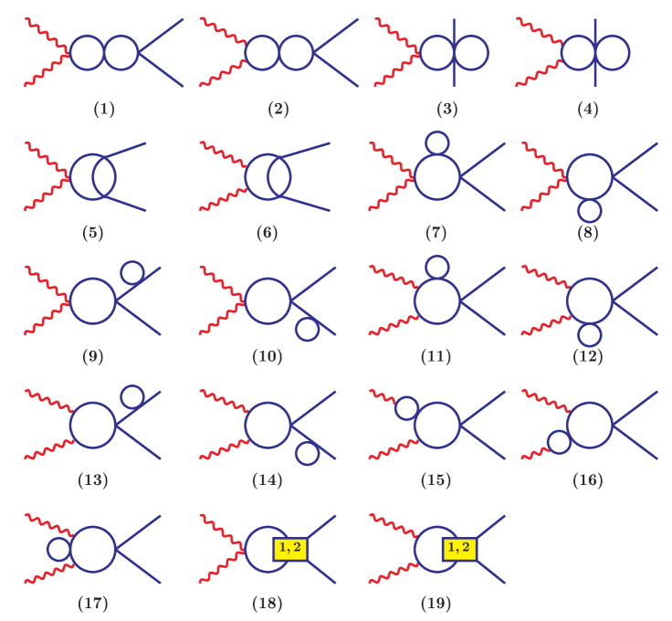
Figure 1: A set of two-loop diagrams generated by ${\mathcal{L}}_{2}$ and one-loop diagrams generated by ${{\mathcal{L}}_{4}.}$

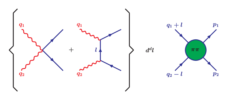
Figure 2: Construction scheme for the diagrams in Fig. 1.

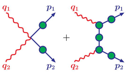
Figure 3: A class of one-particle reducible diagrams. The filled in circles summarize self-energy and vertex corrections.

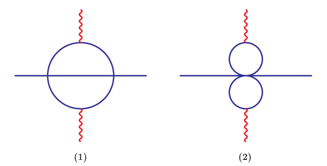
Figure 4: Acnode and butterfly diagrams.

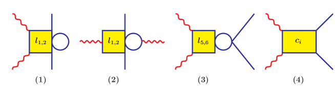
Figure 5: The remaining diagrams at order $p^{6}$: one-loop graphs generated by ${\mathcal{L}}_{4}$, and counterterm contributions from ${\mathcal{L}}_{6}$.

5 The two-loop amplitudes

We give the expressions for the amplitudes $A$ and $B$ using the same notation as in [4]. This results in

$$A=\frac{1}{M_{\pi}^{2}-t}+\frac{1}{M_{\pi}^{2}-u}+\frac{2}{F_{\pi}^{2}}\left\{\bar{G}_{\pi}(s)+\frac{\bar{l}_{\Delta}}{48\pi^{2}}\right\}+U_{\scriptscriptstyle{A}}+P_{\scriptscriptstyle{A}}+{\mathcal{O}}(p^{4}).$$ (5.1)

The unitary part $U_{\scriptscriptstyle{A}}$ contains $s$, $t$ and $u$– channel cuts, and $P_{\scriptscriptstyle{A}}$ is a linear polynomial in $s$. Explicitly we find,

$$U_{\scriptscriptstyle{A}}=\frac{1}{sF_{\pi}^{4}}\bar{G}(s)\;\left[\;(2M_{\pi}^{4}-4M_{\pi}^{2}s+3s^{2})\bar{J}(s)+C(s,\bar{l}_{i})\;\right]\;+\frac{\bar{l}_{\Delta}}{48\pi^{2}F_{\pi}^{4}}s\bar{J}(s)$$

$$+\frac{(\bar{l}_{1}-\frac{4}{3})}{288\pi^{2}sF_{\pi}^{4}}(s-4M_{\pi}^{2})\left\{\bar{H}(s)+4\;[\;s\bar{G}(s)+2M_{\pi}^{2}(\stackrel{{\scriptstyle=}}{{G}}(s)-3\stackrel{{\scriptstyle=}}{{J}}(s))\;]\;d_{00}^{2}\right\}$$

$$+\;\frac{(\bar{l}_{2}-\frac{5}{6})}{96\pi^{2}sF_{\pi}^{4}}\;(s-4M_{\pi}^{2})\left\{\bar{H}(s)+4\;[\;s\bar{G}(s)+2M_{\pi}^{2}(\stackrel{{\scriptstyle=}}{{G}}(s)-3\stackrel{{\scriptstyle=}}{{J}}(s))\;]\;d_{00}^{2}\right\}\vspace{.5cm}$$

$$+\;\Delta_{\scriptscriptstyle{A}}(s,t,u)\;,$$ (5.2)

with

$$C(s,\bar{l}_{i}) = \frac{1}{48\pi^{2}}\left\{\frac{1}{3}\left(\bar{l}_{1}-\frac{4}{3}\right)(16s^{2}-56M_{\pi}^{2}s+64M_{\pi}^{4})\right.$$

$$+\left(\bar{l}_{2}-\frac{5}{6}\right)(8s^{2}-24M_{\pi}^{2}s+32M_{\pi}^{4})$$

$$\left.-12M_{\pi}^{4}\bar{l}_{3}+12M_{\pi}^{2}s\bar{l}_{4}-12M_{\pi}^{2}s+12M_{\pi}^{4}\right\}\;,$$

$$d_{00}^{2} = \frac{1}{2}(3\cos^{2}\theta-1)\;.$$ (5.3)

The loop functions $\bar{J}$ etc. are displayed in Appendix B, and $\bar{G}_{\pi}(s)$ in Eq. (5.1) stands for $\bar{G}(s)$ evaluated with the physical mass. The term proportional to $d_{00}^{2}$ in $U_{\scriptscriptstyle{A}}$ contributes to $D$–waves only. For $\Delta_{\scriptscriptstyle{A}}$ see below. The polynomial part is

$$P_{\scriptscriptstyle{A}} = \frac{1}{(16\pi^{2}F_{\pi}^{2})^{2}}\,\left[\,a_{1}M_{\pi}^{2}+a_{2}s\,\right]\,\;,$$

$$a_{1} = a_{1}^{r}+\frac{1}{9}\left\{4\,l^{2}+l\,\left(-10\,\bar{l}_{1}+18\,\bar{l}_{2}-12\,\bar{l}_{\Delta}+\frac{337}{6}\right)\right.$$

$$\left.-\frac{5}{3}\,\bar{l}_{1}-5\,\bar{l}_{2}+12\,\bar{l}_{4}\bar{l}_{\Delta}+4\right\}\;,$$

$$a_{2} = a_{2}^{r}-\frac{1}{9}\left\{l^{2}+l\,\left(\frac{1}{2}\,\bar{l}_{1}+\frac{3}{2}\,\bar{l}_{2}+3\,\bar{l}_{\Delta}+\frac{127}{24}\right)\right.$$ (5.4)

$$\left.-\frac{5}{12}\,\bar{l}_{1}-\frac{5}{4}\,\bar{l}_{2}+3\,\bar{l}_{\Delta}+\frac{21}{2}\right\}.$$

The result for $B$ reads

$$B=\frac{1}{2s}\left\{\frac{1}{M_{\pi}^{2}-t}+\frac{1}{M_{\pi}^{2}-u}\right\}+U_{\scriptscriptstyle{B}}+P_{\scriptscriptstyle{B}}+{\mathcal{O}}(p^{2})\;,$$ (5.5)

with the unitary part

$$U_{\scriptscriptstyle{B}} = \frac{1}{192\pi^{2}sF_{\pi}^{4}}\left\{\frac{1}{3}\left(\bar{l}_{1}-\frac{4}{3}\right)+\left(\bar{l}_{2}-\frac{5}{6}\right)\right\}\bar{H}(s)+\Delta_{\scriptscriptstyle{B}}(s,t,u)\;.$$ (5.6)

For the polynomial part we find

$$P_{\scriptscriptstyle{B}} = \frac{b}{(16\pi^{2}F_{\pi}^{2})^{2}}\;,$$

$$b = b^{r}-\frac{1}{18}\left\{l^{2}+l\,\left(\frac{1}{2}\,\bar{l}_{1}+\frac{3}{2}\,\bar{l}_{2}-\frac{53}{24}\right)-\frac{1}{12}\,\bar{l}_{1}-\frac{1}{4}\bar{l}_{2}+\frac{7}{2}\right\}\;.$$ (5.7)

The integrals $\Delta_{\scriptscriptstyle{A,B}}(s,t,u)$ contain contributions from the two-loop box, vertex and acnode graphs and also from the reducible diagrams. The explicit expressions for these quantities are given in Appendices C and D .

As an application of the above, we plot the total cross section in Fig. 6, using the LECs from Eqs. (3.10) - (3.12). The data are taken from [25]. It is seen that the two-loop corrections are tiny in this kinematical region.

In order not to interrupt the argument, a detailed comparison of our result with the previous calculation performed by Burgi [4] is relegated to Appendix A.

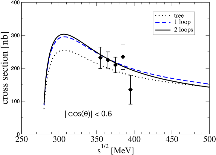
Figure 6: The $\gamma\gamma\to\pi^{+}\pi^{-}$ cross section $\sigma(s;\,|\cos\theta|\leq Z=0.6)$ as a function of $\sqrt{s}$. The experimental data are taken from [25].

6 Pion polarizabilities: dipole and quadrupole

The dipole and quadrupole polarizabilities are defined [26, 27] through the expansion of the helicity amplitudes at fixed $t=M_{\pi}^{2}$,

$$\frac{\alpha}{M_{\pi}}H_{+\mp}(s,t=M_{\pi}^{2})=(\alpha_{1}\pm\beta_{1})_{\pi^{+}}+\frac{s}{12}(\alpha_{2}\pm\beta_{2})_{\pi^{+}}+{\mathcal{O}}(s^{2})\,,$$ (6.1)

where $H_{+\mp}$ denote the helicity amplitudes ${\bar{H}}_{+\mp}$ with Born-term subtracted. Because we have at our disposal the helicity amplitudes at two-loop order, we can work out the polarizabilities to the same accuracy. It turns out that all relevant integrals can be performed in closed form. We discuss the results in the remaining part of this Section.

6.1 Chiral expansion

Using the same notation as in [4], we find for the dipole polarizabilities

$$(\alpha_{1}\pm\beta_{1})_{\pi^{+}}=\frac{\alpha}{16\,\pi^{2}\,F_{\pi}^{2}\,M_{\pi}}\,\left\{c_{1\pm}+\frac{M_{\pi}^{2}\,d_{1\pm}}{16\,\pi^{2}\,F_{\pi}^{2}}+O(M^{4}_{\pi})\right\}\,,$$ (6.2)

where

$$c_{1+} = 0,\qquad c_{1-}=\frac{2}{3}\,\bar{l}_{\Delta}\,,$$

$$d_{1+} = 8\,b^{r}-\frac{4}{9}\left\{l\,\left(l+\frac{1}{2}\,\bar{l}_{1}+\frac{3}{2}\,\bar{l}_{2}\right)-\frac{53}{24}\,l+\frac{1}{2}\,\bar{l}_{1}+\frac{3}{2}\,\bar{l}_{2}+\frac{91}{72}+\Delta_{+}\right\}\;\;,$$

$$d_{1-} = a_{1}^{r}+8\,b^{r}-\frac{4}{3}\left\{l\left(\bar{l}_{1}-\bar{l}_{2}+\bar{l}_{\Delta}-\frac{65}{12}\right)-\frac{1}{3}\,\bar{l}_{1}-\frac{1}{3}\,\bar{l}_{2}+\frac{1}{4}\,\bar{l}_{3}-\bar{l}_{\Delta}\bar{l}_{4}\right.$$ (6.3)

$$\left.+\frac{187}{108}+\Delta_{-}\right\}\,,$$

with

$$\Delta_{+} = \frac{8105}{576}-\frac{135}{64}\,\pi^{2}\,,\qquad\Delta_{-}=\frac{41}{432}-\frac{53}{64}\,\pi^{2}\,.$$ (6.4)

For the quadrupole polarizabilities, we obtain

$$(\alpha_{2}\pm\beta_{2})_{\pi^{+}}=\frac{\alpha}{16\,\pi^{2}\,F_{\pi}^{2}\,M_{\pi}^{3}}\,\left\{c_{2\pm}+\frac{M_{\pi}^{2}d_{2\pm}}{16\,\pi^{2}\,F_{\pi}^{2}}+O(M^{4}_{\pi})\right\}\,,$$ (6.5)

with

$$c_{2+} = 0\,,\qquad c_{2-}=2\,,$$

$$d_{2+} = -\frac{2062}{27}+\frac{10817}{1440}\,\pi^{2}+\frac{8}{45}\,\bar{l}_{1}+\frac{8}{15}\,\bar{l}_{2}\,,$$

$$d_{2-} = 12\,a_{2}^{r}-24\,b^{r}-\,l\,(10+4\,\bar{l}_{\Delta})-\frac{8}{15}\,\bar{l}_{3}+4\,\bar{l}_{4}-4\,\bar{l}_{\Delta}-\frac{218}{45}\,\bar{l}_{1}-\frac{238}{45}\,\bar{l}_{2}$$ (6.6)

$$-\,\frac{56}{45}-\frac{1199}{1920}\,\pi^{2}\,.$$

We end this subsection by evaluating the polarizabilities, using the above expressions and the central values for the LECs in Eqs. (3.10)-(3.12). The results are shown in Table 1. The numbers in brackets correspond to the order $p^{6}$ LECs in Eq. (3.13). The uncertainties are discussed in the following subsection.

Table 1: The dipole and quadrupole polarizabilities. The numbers in brackets correspond to the order $p^{6}$ LECs in Eq. (3.13).

	to one loop	to two-loops
$(\alpha_{1}-\beta_{1})_{\pi^{+}}$	$6.0$	$5.7\,\,[5.5]$
$(\alpha_{1}+\beta_{1})_{\pi^{+}}$	$0$	$0.16\,\,[0.16]$
$(\alpha_{2}-\beta_{2})_{\pi^{+}}$	$11.9$	$16.2\,\,[21.6]$
$(\alpha_{2}+\beta_{2})_{\pi^{+}}$	$0$	$-0.001\,\,[-0.001]$

6.2 Estimating the uncertainties

The uncertainty in the prediction for the polarizability has two sources. First, the low-energy constants are not known precisely. Second, we are dealing here with an expansion in powers of the momenta and of the quark masses. We carried out this expansion up to and including terms of order $p^{6}$. Higher order terms will influence the result - by which amount?

We start the discussion by considering the uncertainties in the LECs. We shall use the order $p^{4}$ LECs displayed in Eqs. (3.10) and (3.11). The LECs at order $p^{6}$ are not well known, see the discussion in Section 3. In Table 2, we display the contributions from the LECs at order $p^{6}$ to the four polarizabilities, using the values from Eq. (3.12). The ones corresponding to Ref. [16] - displayed in Eq. (3.13) - are given in square brackets. The only significant difference occurs in the value of the difference of the quadrupole polarizabilities $(\alpha_{2}-\beta_{2})_{\pi^{\pm}}$.

Table 2: The contribution of the LECs at order $p^{6}$ to the polarizabilities, according to Eq. (3.12). The numbers in brackets correspond to Eq. (3.13).

	$a_{1}^{r}$	$a_{2}^{r}$	$b^{r}$	total
$(\alpha_{1}-\beta_{1})_{\pi^{\pm}}$	$-0.14\,\,[-0.37]$	$0$	$0.14\,\,[0.13]$	$0\,\,[-0.24]$
$(\alpha_{1}+\beta_{1})_{\pi^{\pm}}$	$0$	$0$	$0.14\,\,[0.13]$	$0.14\,\,[0.13]$
$(\alpha_{2}-\beta_{2})_{\pi^{\pm}}$	$0$	$0.72\,\,[6.09]$	$-0.83\,\,[-0.78]$	$-0.10\,\,[5.31]$
$(\alpha_{2}+\beta_{2})_{\pi^{\pm}}$	$0$	$0$	$0$	$0$

Table 3: Resonance saturation induces a scale dependence in the amplitudes. Displayed are the values of the polarizabilities in case that saturation is assumed at $\mu=500$ MeV or at $\mu=1$ GeV.

	$\mu=500$ MeV	$\mu=1$ GeV
$(\alpha_{1}-\beta_{1})_{\pi^{\pm}}$	$6.1$	$5.5$
$(\alpha_{1}+\beta_{1})_{\pi^{\pm}}$	$0.20$	$0.13$
$(\alpha_{2}-\beta_{2})_{\pi^{\pm}}$	$14.6$	$17.2$
$(\alpha_{2}+\beta_{2})_{\pi^{\pm}}$	$-0.001$	$-0.001$

Resonance saturation generates a second inherent uncertainty - should one saturate at $\mu=500$ MeV or at $\mu=1$ GeV? In Table 3 we display the polarizabilities for saturation at these two scales, using Eq. (3.12). It is seen that the induced change (which is independent of the values of the LECs at order $p^{6}$) is quite substantial for $(\alpha_{2}-\beta_{2})_{\pi^{\pm}}$. This is related to the fact that this quantity contains a rather substantial chiral logarithm, see below.

We now discuss the second source of uncertainties, the truncation of the chiral expansion itself. It is clear that, to have an idea of higher order terms, one needs at least the first two terms in the expansion. This makes it already clear that it is difficult to make reliable predictions for the polarizabilities connected with the helicity flip amplitude, from which we have determined here the leading order contribution only. So, let us concentrate first on the helicity non-flip case $H_{++}$.

The Born-term subtracted helicity amplitude $H_{++}$ does not have branch points at the Compton threshold. This is why it can be expanded there into an ordinary Taylor series e.g. in the variable $s$ and $\nu=(t-u)$. One then expects that the amplitude at the Compton threshold is less affected by chiral logarithms than its counterparts at the threshold for $\gamma\gamma\to\pi\pi$, where unitarity cusps do occur. This is illustrated in Fig. 7, where we display the quantity $10^{2}M_{\pi}^{2}H_{++}(s,t=u)$ as a function of $s$ at $t=u$. Above the threshold $s=4M_{\pi}^{2}$, the modulus is shown. The solid (dashed) line is the expression to two loops (to one loop). It is clearly seen that the corrections at the Compton threshold are much smaller than the ones at the threshold for $\gamma\gamma\to\pi\pi$. To identify the chiral logarithms, we note that according to Eq. (3.9), the quantities ${\bar{l}}_{i}$ diverge in the chiral limit, ${\bar{l}}_{i}=-l+\Delta^{r}_{i}$, where $\Delta^{r}_{i}$ is quark mass independent. We decompose the ${\bar{l}}_{i}$ in the amplitude $H_{++}$ in this manner and display the contributions from the chiral logarithms $l$ in Table 4. The numbers illustrate that, indeed, chiral logarithms generate a smaller contribution at the Compton threshold than at threshold for pion pair production.

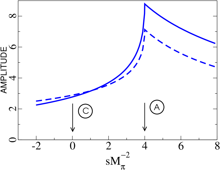
Figure 7: The helicity non-flip amplitude $H_{++}$ in units of $M_{\pi}^{2}$ as a function of $s$, at $t=u$, with Born term subtracted. For $s\leq 4M_{\pi}^{2}$ the quantity shown is $10^{2}M_{\pi}^{2}H_{++}$, and for $s\geq 4M_{\pi}^{2}$ we display $10^{2}M_{\pi}^{2}|H_{++}|$. The solid (dashed) line is the expression to two loops (to one loop). The Compton threshold in $\gamma\pi^{\pm}\to\gamma\pi^{\pm}$ and the threshold in $\gamma\gamma\to\pi^{+}\pi^{-}$ are denoted by the encircled letters $C$ and $A$, respectively. It is clearly seen that two-loop corrections are suppressed at the Compton threshold.

Table 4: The amplitude $10^{2}M_{\pi}^{2}H_{++}(s,t=u)$ at the Compton threshold $s=0$ and at $s=4M_{\pi}^{2}$. The contribution from chiral logarithms, listed in the fourth column, is included in the two-loop result quoted in column three. The normalization is $N_{H}=10^{2}M_{\pi}^{2}$. The LECs at order $p^{6}$ are the ones from Eq. (3.12).

$N_{H}H_{++}(s,t=u)$	to 1 loop	to 2 loops	chiral logarithms
$s=0$	$2.89$	$2.77$	$-0.35$
$s=4M_{\pi}^{2}$	$7.13$	$8.80$	$1.28$

As for the quadrupole polarizabilities $(\alpha_{2}-\beta_{2})_{\pi^{\pm}}$, also connected with the non-flip amplitude, it is seen from Table 1 that there is a substantial two-loop correction to the one-loop result. This can be again understood from the behavior of $H_{++}$. As its value is considerably increased at the threshold $\gamma\gamma\to\pi\pi$, its slope at the Compton threshold receives a substantial correction as well, in order to make up that change. Indeed, the chiral expansion generates chiral logarithms that are responsible for the major part of the increase. If we decompose $(\alpha_{2}-\beta_{2})_{\pi^{\pm}}$ in a manner analogous the amplitude $H_{++}$ above, we find that chiral logarithms contribute with $\simeq 4.5\times 10^{-4}\,{\rm fm}^{5}$ at two-loop order. These logarithms are, of course, independent of the LECs at order $p^{6}$.

Finally, we have checked whether there are potentially large contribution to $H_{++}$ at order $p^{8}$. Using the same procedure as in [5], we found that all contributions from resonance exchange with masses below 1 GeV have a negligible effect - we do not quote the corresponding numbers here.

We now turn to the helicity flip amplitude $H_{+-}$, which starts out at order $p^{6}$: we have determined here only its leading order term in the chiral expansion. We checked whether there are potentially large contribution to $H_{+-}$ at order $p^{8}$, as is the case in $\gamma\gamma\to\pi^{0}\pi^{0}$ [5]. Whereas, there is substantial contribution from $\omega$-exchange in the neutral case, this resonance does not contribute here, and the remaining contributions from $\rho$-exchange are very small, except for the contribution to the slope, parametrized by $(\alpha_{2}+\beta_{2})_{\pi^{\pm}}$, which is affected by $-0.04\times 10^{-4}$ fm⁵. On the other hand, there are also contributions from one-loop graphs at order $p^{8}$, where each vertex is generated by an anomalous contribution $\gamma\pi\to\pi\pi$ from the Wess-Zumino-Witten Lagrangian at order $p^{4}$. We see no reason why these should be small compared to the leading term at order $p^{6}$. We, therefore, do not consider the chiral prediction for these quantities particularly reliable.

6.3 Values of the polarizabilities

We have now all ingredients to provide a value for the polarizabilities in the chiral expansion, and start the discussion with $(\alpha_{1}-\beta_{1})_{\pi^{\pm}}$. We add the uncertainties from the couplings at order $p^{4}$, from $b^{r}$ and from the scale dependence introduced by the resonance scheme in quadrature and obtain

$$\Delta=0.80\times 10^{-4}\,{\mbox{fm}}^{3}\,$$ (6.7)

for the so generated uncertainty.

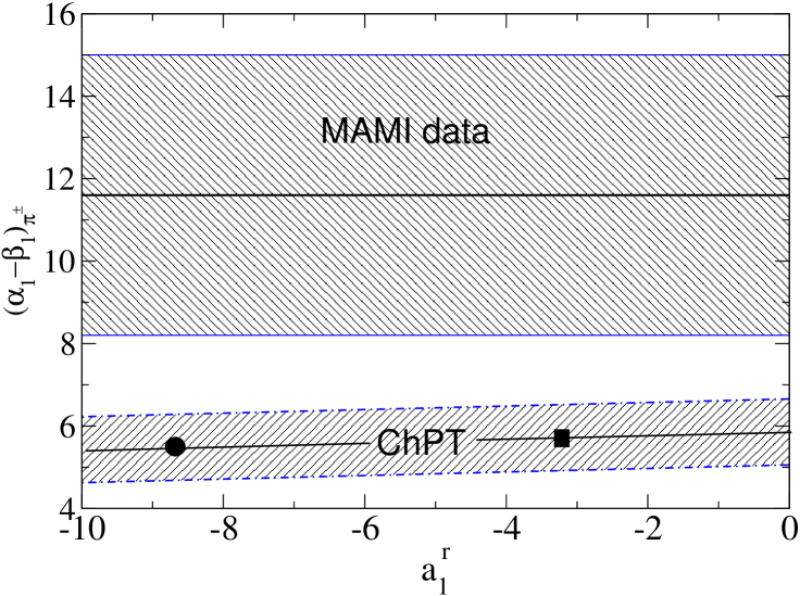
Figure 8: The polarizabilities $(\alpha_{1}-\beta_{1})_{\pi^{\pm}}$ at two-loop order, as a function of $a_{1}^{r}$. The filled in square [filled in circle] denotes the value obtained by using for $a_{1}^{r}$ the value from Eq. (3.12) [(3.13)]. The width of the ChPT band is calculated in the manner described in the text. “MAMI data” refers to the recent MAMI experiment [8]. We have added the errors quoted there in quadrature.

We display in Fig. 8 the result as a function of the rather inaccurately known coupling $a_{1}^{r}$. We indicate with a filled square [filled circle] the two-loop result, evaluated with the LECs given in Eq.(3.12) [3.13]. The width of the band is twice the uncertainty displayed in Eq. (6.7). Let us note that the two-loop prediction differs only slightly from the one-loop calculation, see Table 1. This again shows that the value for the dipole polarizability is rather reliable - there is no sign of any large, uncontrolled correction to the two-loop result. We use the maximum deviation $1.0$ from the central value $5.7$ as the final theoretical uncertainty for the dipole polarizability, and obtain

$$(\alpha_{1}-\beta_{1})_{\pi^{\pm}}=(5.7\pm 1.0)\times 10^{-4}\,{\rm fm}^{3}\,.$$ (6.8)

In the same figure, we also show the result of the recent measurement at MAMI [8] of this quantity. It is seen that the chiral expansion is in conflict with that measurement, independent of any reasonable value chosen for $a_{1}^{r}$. The discrepancy with the recent dispersive analysis by Fil’kov and Kashevarov [10], displayed in Table 5, is even more pronounced.

Table 5: Experimental information on $(\alpha_{1}-\beta_{1})_{\pi^{\pm}}$, in units of $10^{-4}\,{\rm fm}^{3}$. We indicate the reaction and the data used. In [28] and [29], $\alpha_{1}$ was determined, using as a constraint $\alpha_{1}=-\beta_{1}$. To obtain $(\alpha_{1}-\beta_{1})_{\pi^{\pm}}$, we multiplied the results by a factor of 2.

Experiments		$(\alpha_{1}-\beta_{1})_{\pi^{\pm}}$
$\gamma p\to\gamma\pi^{+}n$	Mainz (2005) [8]	$11.6\pm 1.5_{\,\rm stat}\pm 3.0_{\,\rm syst}\pm 0.5_{\,\rm mod}$
L. Fil’kov, V. Kashevarov (2005)  [10]		$13.0^{+2.6}_{-1.9}$
$\gamma\gamma\to\pi^{+}\pi^{-}$	MARK II  [25] ,
TPC/2$\gamma$ [30] ,  CELLO  [31] ,
VENUS  [32] , ALEPH  [33] ,  BELLE [34]
A. Kaloshin, V. Serebryakov (1994)  [35]		$5.25\pm 0.95$
$\gamma\gamma\to\pi^{+}\pi^{-}$	MARK II  [25]
	Crystal Ball Coll. [36]
J.F. Donoghue, B. Holstein (1993)  [28]		$5.4$
$\gamma\gamma\to\pi^{+}\pi^{-}$	MARK II [25]
D. Babusci et al. (1992)  [29]
$\gamma\gamma\to\pi^{+}\pi^{-}$	PLUTO  [37]	$38.2\pm 9.6\pm 11.4$
	DM 1  [38]	$34.4\pm 9.2$
	DM 2  [39]	$52.6\pm 14.8$
	MARK II  [25]	$4.4\pm 3.2$
$\gamma p\to\gamma\pi^{+}n$	Lebedev Inst. (1984) [40]	$40\pm 24$
$\pi^{-}Z\to\gamma\pi^{-}Z$	Serpukhov (1983) [41]	$15.6\pm 6.4_{\,\rm stat}\pm 4.4_{\,\rm syst}$

Next, we discuss the quadrupole case $(\alpha_{2}-\beta_{2})_{\pi^{\pm}}$. Here, the situation differs. First, as we discussed above, chiral logarithms at order $p^{6}$ generate now a rather large contribution. As a result of this, the scale dependence of the saturation scheme is pronounced as well, see Table 3. Second, the LEC $a_{2}^{r}$ enters with weight 12. As a result of this, it now matters which value of $a_{2}^{r}$ is used, even though its contribution is suppressed by the factor ${{M_{\pi}^{2}}(16\pi^{2}F_{\pi}^{2})^{-1}\simeq 0.014}$. Although the effect of using the [16] value for $a_{2}^{r}$ goes in the right direction and brings the result in closer agreement with the analysis of Fil’kov and Kashevarov [10],

$$(\alpha_{2}-\beta_{2})_{\pi^{\pm}}=(25.0^{+0.8}_{-0.3})\times 10^{-4}\,{\rm fm}^{5}\,\,,$$ (6.9)

we cannot take the outcome as a reliable two-loop prediction of ChPT: compared to the one-loop result, the two-loop contribution generates nearly a 100 percent contribution in this case, see Table 1.

As we discussed in the previous subsection, the situation is no better for the polarizabilities $(\alpha_{1,2}+\beta_{1,2})_{\pi^{\pm}}$ associated with the helicity flip amplitude: considerably more work is required to put the chiral prediction on a firm basis. Orders of magnitudes can be read off from Table 1.

In Table 5, we collect experimental information on the dipole polarizabilities of the charged pions. In view of the large scatter of the results, which are partly inconsistent among each other, it is interesting to note that the COMPASS collaboration at CERN is presently remeasuring pion and kaon polarizabilities with high statistics, using the Primakoff effect [42]. It is also worth mentioning that a reanalysis of the MAMI data [8], using a chiral invariant framework, is underway [43].

7 Summary and outlook

1. We have recalculated the two-loop expression for the amplitude $\gamma\gamma\rightarrow\pi^{+}\pi^{-}$ in the framework of chiral perturbation theory. We have made use of the techniques developed in Ref. [5, 23], and of the effective Lagrangian ${\mathcal{L}}_{6}$ constructed in [11, 12].

2. The two Lorentz invariant amplitudes $A$ and $B$ are presented as a sum over multiple Feynman parameter integrals, whose numerical evaluation poses no difficulty. This is in contrast to Ref. [4], where part of the amplitudes, denoted by $\Delta_{A,B}$, could be published in numerical form only. Further, the method has allowed us to evaluate the dipole and quadrupole polarizabilities in closed form. As far as we are aware, the quadrupole polarizabilities for charged pions have never been calculated in ChPT  before.

3. Our result agrees with the earlier calculation [4] up to the remainder $\Delta_{A,B}$. The induced changes in the cross section and in the dipole polarizabilities are far below the uncertainties generated by the (not precisely known) values of the low-energy constants. For the cross section below 500 MeV, the change is less than 1 percent. For the polarizabilities, the change is given in columns two and three of Table 6.

4. We have investigated the uncertainties in the polarizabilities due to higher order corrections, and due to the uncertainties in the LECs at order $p^{6}$. According to our analysis, the two-loop result Eq. (6.8) for the dipole polarizability $(\alpha_{1}-\beta_{1})_{\pi^{\pm}}$ is particularly reliable. It is in conflict with the recent experimental result obtained at MAMI [8], or with the dispersive analysis performed in [10].

Appendix A Comparison with the previous calculation

In this appendix, we compare the amplitudes $A,B$ and the dipole polarizabilities with the previous calculation presented in Ref. [4]. In that reference, the amplitudes were evaluated with a different technique. Furthermore, the Lagrangian ${\mathcal{L}}_{6}$ was not available in those days, and an important ingredient to check the final result was, therefore, missing. We can make the following observations.

1. The amplitudes $A$ and $B$ consist of a part with explicit analytic expressions, and additional terms $\Delta_{A,B}$, that are displayed in Appendices C and D of the present work in the form of integrals over Feynman parameters. $\Delta_{A,B}$ were given only in numerical form in [4].

2. We find that our explicit analytic expressions agree with the ones in [4]. To compare $\Delta_{A,B}$, we made two checks. First, we evaluated the cross section for the reaction $\gamma\gamma\rightarrow\pi^{+}\pi^{-}$ below a centre-of-mass energy of 500 MeV, using the same values for the LECs as in [4],

   $$(\bar{l}_{1},\bar{l}_{2},\bar{l}_{3},\bar{l}_{4},\bar{l}_{\Delta}) = (-1.7,6.1,2.9,4.3,2.7)\,,$$

   $$(a_{1}^{r},a_{2}^{r},b^{r}) = (-3.3,0.75,0.45)\,.$$ (1.1)

   Our result agrees within a fraction of a percent with the two-loop result displayed in Fig. 9 of Ref. [4].

3. Second, we evaluated the dipole polarizabilities by using the values of the LECs in Eq. (2). The result is displayed in the third column of Table 6. In the second column, we display the values obtained in [4]. It is seen that the two results agree very well. The small difference is entirely due to the slightly different values of the quantities $\Delta_{A,B}$.

Table 6: Comparison of the polarizabilities with the previous calculation by Burgi [4]. The second column displays Burgi’s result, the third one our evaluation, using Eq. (2). The fourth column displays the polarizabilities evaluated with the LECs used in the present work.

	Burgi [4]	Present work	Present work
		LECs from Eq. (2)	LECs from Eqs. (3.10) - (3.12)
$(\alpha_{1}-\beta_{1})_{\pi^{+}}$	$4.42$	$4.39$	$5.72$
$(\alpha_{1}+\beta_{1})_{\pi^{+}}$	$0.31$	$0.28$	$0.16$

The following comments concerning the central values of the polarizabilities are in order. We display in the last column in Table 6 the values of polarizabilities obtained by using the LECs from Eqs. (3.10) - (3.12). It is seen that the combination $(\alpha_{1}-\beta_{1})_{\pi^{\pm}}$ differs considerably from the one obtained with Eq. (2). To identify the source of this difference, we first note that the polarizabilities depend linearly on the LECs, except the term $\bar{l}_{\Delta}\bar{l}_{4}$ in $d_{1-}$, as can be seen from the Eqs. (6.2-6.4). We then expand $(\alpha_{1}-\beta_{1})_{\pi^{\pm}}$ in the LECs around their central values, drop quadratic terms and obtain at $\mu=M_{\rho}$ the decomposition

$$(\alpha_{1}-\beta_{1})_{\pi^{\pm}} = 5.719$$ (1.2)

$$+ 0.215\cdot(\bar{l}_{1}+0.4)-0.177\cdot(\bar{l}_{2}-4.3)-0.014\cdot(\bar{l}_{3}-2.9)$$

$$+ 0.172\cdot(\bar{l}_{4}-4.4)+2.44\cdot(\bar{l}_{\Delta}-3)+0.04\cdot(a_{1}^{r}+8b^{r})\,.$$

Inserting in this expansion e.g. the values in Eq. (2) generates the result in column 3 of Table 6. It turns out that all changes in the order $p^{4}$ LECs have conspired to modify Burgi’s result for $(\alpha_{1}-\beta_{1})_{\pi^{\pm}}$ towards positive values. The contribution from the LECs at order $p^{6}$ is negligible.

In summary, we conclude that our calculation nicely confirms Burgi’s result [4], provided that the same set of LECs is used.

Appendix B One-loop functions

In order to simplify the expressions, we set the pion mass equal to one in the following Appendices,

$$M_{\pi}=1\,.$$ (2.3)

1. The loop-integral $\bar{G}(s)$ is

$$\bar{G}(s)=-\frac{1}{16\pi^{2}}\left\{1+\frac{2}{s}\int^{1}_{0}\frac{dx}{x}\ln(1-s\,x(1-x))\right\}\;.$$ (2.4)

$\bar{G}$ is analytic in the complex $s$ - plane, cut along the positive real axis for Re $s\geq 4$. At small $s$,

$$\bar{G}(s)=\frac{1}{16\pi^{2}}\sum_{n=1}^{\infty}s^{n}\frac{(n!)^{2}}{(n+1)(2n+1)!}\;.$$ (2.5)

The absorptive part is

$$\mbox{Im}\,\bar{G}(s) = \frac{1}{8\,s\,\pi}\ln\left\{\frac{1+\sigma}{1-\sigma}\right\}\,,\hskip 28.45274pts>4\,,$$

$$\sigma = \sqrt{1-4/s}\,,$$ (2.6)

and

$$-16\pi^{2}\bar{G}(s)=\left\{\begin{array}[]{lll}1&+\frac{1}{s}\left(\ln\frac{1-\sigma}{1+\sigma}+i\pi\right)^{2};&\qquad 4\leq s\,,\\ 1&-\frac{4}{s}\mbox{arctg}^{2}(\frac{s}{4-s})^{\frac{1}{2}}\,;&\qquad 0\leq s\leq 4\,,\\ 1&+\frac{1}{s}\ln^{2}\frac{\sigma-1}{\sigma+1}\,;&\qquad s\leq 0\,.\end{array}\right.$$ (2.7)

In the text we also need

$$\stackrel{{\scriptstyle=}}{{G}}(s) = \bar{G}(s)-s\,\bar{G}^{\prime}(0)\,.$$ (2.8)

2. The loop-integral $\bar{J}(s)$ is

$$\bar{J}(s)=-\frac{1}{16\pi^{2}}\int_{0}^{1}dx\ln(1-s\,x(1-x))\;.$$ (2.9)

$\bar{J}$ is analytic in the complex $s$ - plane, cut along the positive real axis for Re $s\geq 4$. At small $s$,

$$\bar{J}(s)=\frac{1}{16\pi^{2}}\sum_{n=1}^{\infty}s^{n}\frac{(n!)^{2}}{n(2n+1)!}\;.$$ (2.10)

The absorptive part is

$$\mbox{Im}\,\bar{J}(s)=\frac{\sigma}{16\pi}\,,\hskip 28.45274pts>4\;.$$ (2.11)

Explicitly,

$$16\pi^{2}\bar{J}(s)=\left\{\begin{array}[]{lll}&\sigma\left(\ln\frac{1-\sigma}{1+\sigma}+i\pi\right)+2\,;&\qquad 4\leq s\,,\\ &2-2(\frac{4-s}{s})^{\frac{1}{2}}\mbox{arctg}(\frac{s}{4-s})^{\frac{1}{2}}\,;&\qquad 0\leq s\leq 4\,,\\ &\sigma\ln\frac{\sigma-1}{\sigma+1}+2\,;&\qquad s\leq 0\,.\end{array}\right.$$ (2.15)

In the text we also need

$$\stackrel{{\scriptstyle=}}{{J}}(s) = \bar{J}(s)-s\,\bar{J}^{\prime}(0)\,.$$ (2.16)

3. The loop-function $\bar{H}$ is defined in terms of $\bar{G}$ and $\bar{J}$,

$$\bar{H}(s)=(s-10)\bar{J}(s)+6\,\bar{G}(s)\,.$$ (2.17)

Appendix C The quantities $\Delta_{A}$ and $\Delta_{B}$

Here we display the expressions for the quantities $\Delta_{A(B)}$.

$$\Delta_{A}(s,t,u)=\frac{1}{(4\pi F_{\pi})^{4}}\left\{\left(\frac{35947}{8100}+\frac{\pi^{2}}{3}\right)-\frac{1130291}{6350400}s-S(t)-S(u)\right\}$$

$$\hskip 28.45274pt+\frac{1}{(4\pi F_{\pi})^{4}}\frac{1}{288}\left\{F_{A}^{\rm acn}(s,t,u)+F_{A}^{\rm ver}(s)+F_{A}^{\rm box}(s,t,u)\right\},$$ (3.18)

$$\Delta_{B}(s,t,u)=\frac{1}{(4\pi F_{\pi})^{4}}\left\{\frac{492197}{1411200}-\left(\frac{81101}{70560}-\frac{\pi^{2}}{6}+\frac{1}{2}S(t)+\frac{1}{2}S(u)\right)\frac{1}{s}\right\}$$

$$\hskip 28.45274pt+\frac{1}{(4\pi F_{\pi})^{4}}\frac{1}{576}\left\{F_{B}^{\rm acn}(s,t,u)+F_{B}^{\rm ver}(s)+F_{B}^{\rm box}(s,t,u)\right\}.$$ (3.19)

Here, the function $S(t)$ is defined by

$$S(t) = \frac{h_{F}(t)}{6(t-1)^{2}}\,,$$ (3.20)

$$h_{F}(t) = -\int\limits_{4}^{\infty}d\sigma\beta(\sigma)\int_{0}^{1}dx\left\{6t+(1-12x+18x^{2})t^{2}\right\}$$

$$\times\left\{\ln\frac{z_{2}(x,t)}{z_{2}(x,1)}+\frac{(t-1)x(1-x)}{z_{2}(x,1)}\right\}\,,$$

$$\beta(\sigma) = \sqrt{1-4/\sigma}\,,$$

$$z_{2}(x,t) = x^{2}+\sigma(1-x)-(t-1)x(1-x)\,.$$

The loop function $h_{F}(t)$ stems from the sunset diagram. The functions $F_{I}$ are stemming from the acnode, vertex and box diagrams and are defined by

$$F_{I}^{\rm acn} = \int\limits_{4}^{\infty}\!d\sigma\beta\!\int\limits_{0}^{1}\!d^{3}x\left\{\frac{P_{I;\,{\rm acn}(1)}}{y\cdot z_{{\rm acn}(1)}}+\sum\limits_{i=2}^{6}\frac{P_{I;\,{\rm acn}(i)}}{z^{2}_{{\rm acn}(i)}}\right\}\,,$$

$$F_{I}^{\rm ver} = \int\limits_{4}^{\infty}\!\frac{d\sigma\beta}{\sigma}\!\int\limits_{0}^{1}\!d^{2}x\cdot\frac{P_{I;{\rm ver}}}{z_{\rm ver}}\,,$$

$$F_{I}^{\rm box} = \!\!\int\limits_{4}^{\infty}\!\frac{d\sigma\beta}{\sigma}\int\limits_{0}^{1}\!d^{3}x\sum\limits_{n=1}^{2}\left\{P_{I;\rm{box_{+}}}^{(n)}D^{(n)}_{\rm box_{+}}+P_{I;\rm{box_{-}}}^{(n)}D^{(n)}_{\rm box_{-}}\right\}\,,\quad I=A,B,$$ (3.21)

and

$$D^{(n)}_{\rm box_{\pm}} = \frac{1}{z^{n}_{\rm box;t}}\pm\frac{1}{z^{n}_{\rm box;u}}\,.$$

Here $P_{I}$ are polynomials in $s,\nu=t-u$ and in $x_{i}$. Their explicit expressions are given in Appendix D. The arguments of the functions are defined by

$$z_{{\rm acn}(i)} = y-a_{i}x_{3}(1-x_{3})\,,\qquad(i=1,\ldots,6)\,,\qquad y=x_{3}^{2}+\sigma(1-x_{3})\,,$$

$$a_{1} = a_{2}=x_{1}x_{2}s+x_{1}(t-1)+x_{2}(u-1)\,,$$

$$a_{3} = t-1\,,\quad a_{4}=x_{1}(t-1)\,,$$

$$a_{5} = u-1\,,\quad a_{6}=x_{2}(u-1)\,,$$

$$z_{\rm ver} = \sigma(1-x_{3})+x_{3}^{2}y_{2}\,,\hskip 28.45274pty_{2}=1-sx_{2}(1-x_{2})\,,$$

$$z_{\rm box;t} = B_{\rm t}-A_{\rm t}x_{1}\,,$$

$$A_{\rm t} = x_{2}x_{3}\Big{[}s(1-x_{2})x_{3}+(1-t)(1-x_{3})\Big{]}\,,$$

$$B_{\rm t} = A_{\rm t}+z_{\rm ver}\,,$$

$$z_{\rm box;u} = z_{\rm box;t}|_{t\rightarrow u}\,.$$ (3.22)

The acnode integrals are easy to evaluate numerically in the physical region for the reaction $\gamma\gamma\to\pi\pi$, because branch points occur at $t=4,u=4$ only. On the other hand, the vertex and box integrals contain branch points at $s=4$. In order to evaluate these integrals at $s\geq 4$, we invoke dispersion relations in the manner described in [23].

Appendix D The polynomials $P_{A}$ and $P_{B}$

Here, we display the polynomials $P_{A(B)}$ that occur in the expressions $\Delta_{A(B)}$ in Appendix C. We use the abbreviations

$$x_{+} = x_{1}+x_{2}-2x_{1}x_{2}\,,\qquad x_{-}=x_{1}-x_{2}\,,$$

$$x_{123} = (1+x_{3}-2x_{2}x_{3})(1-x_{3}+2x_{1}x_{2}x_{3})\,.$$ (4.23)

D.1 The polynomials $P_{A}$

$$P_{{\rm A;\,acn}(1)} = \;\;\;144x_{3}(1-x_{3})(sx_{+}-\nu x_{-}),$$

$$P_{{\rm A;acn}(2)} = \;\;\;12s^{2}(1-x_{3})^{2}\Big{\{}x_{+}(5x_{+}+6x_{-}^{2}-1)-5x_{+}^{2}x_{3}-6x_{-}^{2}x_{3}^{2}$$

$$+\Big{[}x_{-}^{2}(9-6x_{+})-x_{+}(2-7x_{+})\Big{]}x_{3}^{3}$$

$$+\Big{[}6x_{-}^{2}(x_{+}-1)+(3-7x_{+})x_{+}\Big{]}x_{3}^{4}\Big{\}}$$

$$+12s\nu(1-x_{3})^{2}x_{-}\Big{\{}1-6x_{-}^{2}-14x_{+}+10x_{+}x_{3}$$

$$+6(1+2x_{-}^{2}-x_{+})x_{3}^{2}-2(6x_{-}^{2}+5x_{+}-1)x_{3}^{3}$$

$$+(6x_{-}^{2}+8x_{+}-3)x_{3}^{4}\Big{\}}$$

$$-12\nu^{2}(1-x_{3})^{2}\Big{\{}6x_{+}(1-2x_{+})x_{3}^{2}$$

$$-x_{-}^{2}\Big{[}9-5x_{3}-12x_{+}x_{3}^{2}-(6-18x_{+})x_{3}^{3}+(5-12x_{+})x_{3}^{4}\Big{]}\Big{\}}$$

$$+24\nu(1-x_{3})x_{-}\Big{\{}1+2x_{+}-(25+2x_{+})x_{3}+3(7-8x_{+})x_{3}^{2}$$

$$+(100x_{+}-41)x_{3}^{3}+(51-118x_{+})x_{3}^{4}+(42x_{+}-19)x_{3}^{5}\Big{\}}$$

$$-12s(1-x_{3})\Big{\{}2x_{+}(1+2x_{+})+2(2-12x_{-}^{2}-17x_{+}-2x_{+}^{2})x_{3}$$

$$+2(13-6x_{-}^{2}-11x_{+})x_{3}^{2}-2(41-18x_{-}^{2}-89x_{+}+8x_{+}^{2})x_{3}^{3}$$

$$+(82-36x_{-}^{2}-194x_{+}+28x_{+}^{2})x_{3}^{4}$$

$$-2(15-6x_{-}^{2}-35x_{+}+6x_{+}^{2})x_{3}^{5}\Big{\}}$$

$$+48x_{3}(1-x_{3})\Big{\{}-2-4x_{+}+(35-50x_{+})x_{3}$$

$$+71(2x_{+}-1)x_{3}^{2}+(61-130x_{+})x_{3}^{3}+2(21x_{+}-10)x_{3}^{4}\Big{\}}\,,$$

$$P_{{\rm A;\,acn}(3)} = \;\;\;3(s-\nu)^{2}(1-x_{3})^{5}(1+x_{3})$$

$$+6(s-\nu)(1-x_{3})^{3}(3+5x_{3}+2x_{3}^{2}-2x_{3}^{3})$$

$$+12x_{3}(1-x_{3})(2-x_{3})(3+3x_{3}+x_{3}^{2}-x_{3}^{3})\,,$$

$$P_{{\rm A;\,acn}(4)} = \;\;\;24(s-\nu)^{2}x_{1}^{2}(1-2x_{1})(1-x_{3})^{4}(2+x_{3})$$

$$+48(s-\nu)x_{1}(1-2x_{1})(1-x_{3})^{2}(2+4x_{3}-3x_{3}^{2})$$

$$+96(1-2x_{1})x_{3}(1-x_{3})(2-x_{3})(2+2x_{3}-x_{3}^{2})\,,$$

$$P_{{\rm A;\,acn}(5)} = \;\;\;P_{{\rm A;\,acn}(3)}|_{\rm t\leftrightarrow u}\,,$$

$$P_{{\rm A;\,acn}(6)} = \;\;\;P_{{\rm A;\,acn}(4)}|_{\rm t\leftrightarrow u,\,x_{1}\leftrightarrow x_{2}}\,,$$

$$P_{\rm A;\,ver} = -8s^{2}(1-2x_{2})x_{2}^{2}x_{3}^{4}\Big{\{}-54+72(3+4x_{2})x_{3}$$

$$+(330-1134x_{2}-811x_{2}^{2})x_{3}^{2}-108(5-15x_{2}^{2}-4x_{2}^{3})x_{3}^{3}$$

$$-45x_{2}(18-75x_{2}+32(3-x_{2})x_{2}^{2})x_{3}^{4}\Big{\}}$$

$$+32s(1-2x_{2})x_{2}^{2}x_{3}^{4}\Big{\{}33+8(27-7x_{2})x_{3}$$

$$-3(222-30x_{2}+55x_{2}^{2})x_{3}^{2}-540(1-3x_{2}+x_{2}^{2})x_{3}^{3}$$

$$+1215(1-x_{2})^{2}x_{3}^{4}\Big{\}}\,,$$

$$P_{\rm A;\,box;+}^{(1)} = \;\;\;4s^{2}x_{2}^{2}x_{3}^{3}\Big{\{}6x_{1}\Big{[}9-2(23+8x_{2})x_{3}-(67-405x_{2}+31x_{2}^{2})x_{3}^{2}$$

$$+(70+39x_{2}-808x_{2}^{2}+20x_{2}^{3})x_{3}^{3}$$

$$+9(6-61x_{2}+53x_{2}^{2}+60x_{2}^{3})x_{3}^{4}-81x_{2}(3-10x_{2}+8x_{2}^{2})x_{3}^{5}\Big{]}$$

$$+3x_{1}^{2}x_{2}x_{3}\Big{[}-92-171x_{3}+592x_{2}x_{3}$$

$$+(231+4(194-339x_{2})x_{2})x_{3}^{2}$$

$$+9(1-2x_{2})(71-22x_{2}-60x_{2}^{2})x_{3}^{3}$$

$$+27(1-2x_{2})^{2}(11-16x_{2})x_{3}^{4}\Big{]}-2x_{1}^{3}x_{2}^{2}x_{3}^{2}\Big{[}245+(1-2x_{2})x_{3}$$

$$\times(470+27(1-2x_{2})x_{3}(15+8(1-2x_{2})x_{3}))\Big{]}$$

$$+6x_{3}(-19+24x_{3}+35x_{3}^{2}-36x_{3}^{3}$$

$$+x_{2}^{2}x_{3}(-25+40x_{3}+27(5-6x_{3})x_{3}^{2})$$

$$+x_{2}(10+44x_{3}-199x_{3}^{2}+9x_{3}^{3}(8+9x_{3})))\Big{\}}$$

$$+12\nu^{2}x_{2}^{3}x_{3}^{4}\Big{\{}-20-16x_{1}(2+7x_{1})$$

$$+\Big{[}48+50x_{2}+310x_{1}+101x_{1}^{2}+30x_{1}(3+15x_{1}-5x_{1}^{2})x_{2}\Big{]}x_{3}$$

$$+\Big{[}-78+2x_{1}+411x_{1}^{2}-20(9+63x_{1}+57x_{1}^{2}+13x_{1}^{3})x_{2}$$

$$+120x_{1}(1+x_{1}+5x_{1}^{2})x_{2}^{2}\Big{]}x_{3}^{2}-3\Big{[}24+3x_{1}(94+73x_{1})$$

$$-2(69+351x_{1}+381x_{1}^{2}+19x_{1}^{3})x_{2}$$

$$+4x_{1}(24+117x_{1}+34x_{1}^{2})x_{2}^{2}\Big{]}x_{3}^{3}$$

$$+9(1-2x_{2})\Big{[}18+54x_{1}-36x_{1}x_{2}+x_{1}^{2}(33-2(9+8x_{1})x_{2})\Big{]}x_{3}^{4}\Big{\}}$$

$$-48sx_{2}x_{3}^{2}\Big{\{}-6+\Big{[}18+20x_{2}-31x_{1}x_{2}\Big{]}x_{3}$$

$$-\Big{[}29+49x_{2}+4x_{2}^{2}+4x_{1}x_{2}(9-(22-8x_{1})x_{2})\Big{]}x_{3}^{2}$$

$$+\Big{[}-6+202x_{2}-54x_{2}^{2}+164x_{1}x_{2}$$

$$+114x_{1}x_{2}^{2}-4x_{1}x_{2}^{3}-x_{1}^{2}x_{2}^{2}(149-58x_{2})\Big{]}x_{3}^{3}$$

$$+\Big{[}65-333x_{2}-40x_{2}^{2}+189x_{1}x_{2}-4x_{1}(137+75x_{2})x_{2}^{2}$$

$$+5x_{1}^{2}x_{2}^{2}(23+12x_{2}(5+x_{2}))\Big{]}x_{3}^{4}$$

$$-9\Big{[}4-46x_{2}^{2}-x_{1}^{2}x_{2}^{2}(1-2x_{2})(41+8x_{2})$$

$$+x_{1}x_{2}(25+18x_{2}-76x_{2}^{2})\Big{]}x_{3}^{5}$$

$$+81x_{2}(1-2x_{2})\Big{[}2-3x_{1}+x_{1}(2+x_{1})x_{2}-2x_{1}^{2}x_{2}^{2}\Big{]}x_{3}^{6}\Big{\}}$$

$$+96x_{2}x_{3}^{2}\Big{\{}-21+\Big{[}36+65(1-x_{1})x_{2}\Big{]}x_{3}$$

$$+\Big{[}23-8(23-x_{1})x_{2}+176x_{1}x_{2}^{2}\Big{]}x_{3}^{2}$$

$$-2\Big{[}6-(83+37x_{1})x_{2}+120x_{1}x_{2}^{2}\Big{]}x_{3}^{3}$$

$$-\Big{[}29+10(17-7x_{1})x_{2}-100x_{1}x_{2}^{2}\Big{]}x_{3}^{4}$$

$$-9\Big{[}8-(31+x_{1})x_{2}+32x_{1}x_{2}^{2}\Big{]}x_{3}^{5}+81(1-\!2\!x_{2})(1-2x_{1}x_{2})x_{3}^{6}\Big{\}}\,,$$

$$P_{\rm A;\,box;-}^{(1)} = \;\;\;-8s\nu x_{2}^{2}x_{3}^{3}\Big{\{}27x_{1}-\Big{[}57+6x_{1}(13+(26+51x_{1})x_{2})\Big{]}x_{3}$$

$$+\Big{[}72-129x_{1}+3(68+x_{1}(456+25x_{1}))x_{2}$$

$$+x_{1}(282+x_{1}(1383-470x_{1}))x_{2}^{2}\Big{]}x_{3}^{2}$$

$$+\Big{[}105+330x_{1}-714x_{2}-3x_{1}(200-489x_{1})x_{2}$$

$$-2(75+x_{1}(1557+912x_{1}+470x_{1}^{2}))x_{2}^{2}$$

$$-120x_{1}(3+9x_{1}-16x_{1}^{2})x_{2}^{3}\Big{]}x_{3}^{3}+9\Big{[}2x_{1}^{3}x_{2}^{2}(1-2x_{2})(13+34x_{2})$$

$$+3x_{1}^{2}x_{2}(1-2x_{2})(1-23x_{2}+4x_{2}^{2})$$

$$-6x_{1}(1-2x_{2})(3+36x_{2}+17x_{2}^{2})-6(2-2x_{2}-19x_{2}^{2})\Big{]}x_{3}^{4}$$

$$+27x_{2}(1-2x_{2})\Big{[}18+18x_{1}x_{2}-33x_{1}^{2}$$

$$+2x_{1}^{2}x_{2}(33-9x_{2}+8x_{1}(1-2x_{2}))\Big{]}x_{3}^{5}\Big{\}}$$

$$+48\nu x_{2}^{2}x_{3}^{3}\Big{\{}18-29x_{1}$$

$$-\Big{[}21+4(10x_{1}+12x_{2}-19(2-x_{1})x_{1}x_{2})\Big{]}x_{3}$$

$$+\Big{[}42+106x_{2}+252x_{1}-23x_{1}^{2}x_{2}(7-10x_{2})$$

$$-6x_{1}x_{2}(3+20x_{2})\Big{]}x_{3}^{2}-\Big{[}83+230x_{2}-41x_{1}$$

$$+5x_{1}x_{2}(134-20x_{2}-3x_{1}(9+10x_{2}))\Big{]}x_{3}^{3}$$

$$-9\Big{[}12-54x_{2}+x_{1}(1-2x_{2})(53-(24+41x_{1})x_{2})\Big{]}x_{3}^{4}$$

$$+81(1-2x_{2})\Big{[}2+3x_{1}-x_{1}(4+x_{1})x_{2}\Big{]}x_{3}^{5}\Big{\}}\,,$$

$$P_{\rm A;\,box;+}^{(2)} = \;\;\;-6s^{3}\Big{[}1+x_{1}(1-2x_{2})\Big{]}x_{2}^{3}x_{3}^{6}x_{123}$$

$$\times\Big{[}8-5x_{2}+8x_{1}-x_{1}(6+5x_{1})x_{2}-6x_{3}$$

$$-6x_{1}(1-2x_{2})x_{3}+9x_{2}(1+x_{1}(1-2x_{2}))^{2}x_{3}^{2}\Big{]}$$

$$-6s\nu^{2}(1-x_{1})^{2}x_{2}^{3}x_{3}^{6}x_{123}$$

$$\times\Big{[}8-6x_{3}+x_{2}(1+x_{1}(1-2x_{2}))(5-3x_{3}(4-9x_{3}))\Big{]}$$

$$+12s^{2}x_{2}^{2}x_{3}^{4}x_{123}\Big{\{}2(2+x_{2}+2x_{1}-(6-x_{1})x_{1}x_{2})$$

$$-12\Big{[}1+x_{1}(1-2x_{2})\Big{]}x_{3}+\Big{[}13(2-x_{2})$$

$$+2x_{1}(1-x_{2})(13-16x_{2})-x_{1}^{2}x_{2}(13-32x_{2}+32x_{2}^{2})\Big{]}x_{3}^{2}$$

$$-12\Big{[}1+x_{1}+x_{2}+x_{1}^{2}(1-2x_{2})^{2}x_{2}-4x_{1}x_{2}^{2}\Big{]}x_{3}^{3}$$

$$+27x_{2}\Big{[}1+x_{1}(1-2x_{2})\Big{]}^{2}x_{3}^{4}\Big{\}}$$

$$-12\nu^{2}(1-x_{1})^{2}x_{2}^{3}x_{3}^{4}x_{123}\Big{\{}2+12x_{3}-17x_{3}^{2}+24x_{3}^{3}-27x_{3}^{4}\Big{\}}$$

$$+24sx_{2}x_{3}^{4}x_{123}\times\Big{\{}6(2-x_{3})(1-x_{3})x_{3}$$

$$+2x_{1}x_{2}^{2}\Big{[}23-24x_{3}+x_{3}^{2}(2-3x_{3})(2-9x_{3})\Big{]}$$

$$+(1+x_{1})x_{2}\Big{[}-23+24x_{3}-4x_{3}^{2}+3(8-9x_{3})x_{3}^{3}\Big{]}\Big{\}}$$

$$+144x_{2}(1-x_{3})^{2}x_{3}^{4}x_{123}\Big{[}5+x_{3}(2+3x_{3})\Big{]}\,,$$

$$P_{\rm A;\,box;-}^{(2)} = \;\;\;6\nu^{3}(1-x_{1})^{3}x_{2}^{4}x_{3}^{6}x_{123}\Big{[}5-6x_{3}+9x_{3}^{2}\Big{]}$$

$$+6s^{2}\nu(1-x_{1})x_{2}^{3}x_{3}^{6}x_{123}\times\Big{\{}16+16x_{1}-5x_{2}-22x_{1}x_{2}-5x_{1}^{2}x_{2}$$

$$-6\Big{[}2+(1+x_{1})x_{2}-2x_{1}x_{2}^{2}\Big{]}\Big{[}1+x_{1}(1-2x_{2})\Big{]}x_{3}$$

$$+27x_{2}\Big{[}1+x_{1}(1-2x_{2})\Big{]}^{2}x_{3}^{2}\Big{\}}$$

$$-24s\nu(1-x_{1})x_{2}^{2}x_{3}^{4}x_{123}\times\Big{\{}2-6x_{3}+(13-6x_{3})x_{3}^{2}$$

$$-x_{2}\Big{[}1+x_{1}(1-2x_{2})\Big{]}\Big{[}6-2x_{3}+9x_{3}^{2}(2-3x_{3})\Big{]}x_{3}\Big{\}}$$

$$+72\nu(1-x_{1})(1-x_{3})x_{2}^{2}x_{3}^{4}x_{123}\Big{[}5-7x_{3}+(1-9x_{3})x_{3}^{2}\Big{]}\,.$$

D.2 The polynomials $P_{B}$

$$P_{{\rm B;\,acn}(1)} = \;\;\;144x_{3}(1-x_{3})\Big{[}x_{+}-\frac{\nu}{s}x_{-}\Big{]}\,,$$

$$P_{{\rm B;\,acn}(2)} = \;\;\;\frac{12\nu^{2}}{s}(1-x_{3})^{2}\Big{[}(3-5x_{3}-x_{3}^{4})x_{-}^{2}+6x_{3}^{2}x_{+}\Big{]}$$

$$+\frac{24\nu x_{-}}{s}(1-x_{3})^{2}(7-12x_{3}+3x_{3}^{2}+4x_{3}^{3}-5x_{3}^{4})$$

$$-\frac{48}{s}x_{3}(1-x_{3})(14+19x_{3}-43x_{3}^{2}+29x_{3}^{3}-10x_{3}^{4})$$

$$+12s(1-x_{3})^{2}\Big{\{}x_{+}(1+3x_{+})-5x_{3}x_{+}^{2}+6x_{3}^{2}x_{-}^{2}$$

$$-x_{3}^{3}\Big{[}9x_{-}^{2}-x_{+}(2+3x_{+})\Big{]}+x_{3}^{4}\Big{[}6x_{-}^{2}-x_{+}(3+x_{+})\Big{]}\Big{\}}$$

$$-12\nu x_{-}(1-x_{3})^{2}\Big{[}1+6x_{+}-10x_{3}x_{+}+6x_{3}^{2}(1+x_{+})$$

$$+2x_{3}^{3}(1-3x_{+})-x_{3}^{4}(3-4x_{+})\Big{]}$$

$$-24(1-x_{3})^{2}\Big{[}7x_{+}-2(1+6x_{+})x_{3}$$

$$-(1-x_{+})x_{3}^{2}(15-26x_{3})-(15-13x_{+})x_{3}^{4}\Big{]}\,,$$

$$P_{{\rm B;\,acn}(3)} = \;\;\;\frac{3(s-\nu)^{2}}{s}(1-x_{3})^{5}(1+x_{3})$$

$$+\frac{6(s-\nu)}{s}(1-x_{3})^{3}\Big{[}3+5x_{3}+2x_{3}^{2}(1-x_{3})\Big{]}$$

$$+\frac{12}{s}x_{3}(1-x_{3})(2-x_{3})\Big{[}3(1+x_{3})+x_{3}^{2}(1-x_{3})\Big{]}\,,$$

$$P_{{\rm B;\,acn}(4)} = -\frac{24(s-\nu)^{2}}{s}x_{1}^{2}(1-x_{3})^{4}(2+x_{3})$$

$$-\frac{48(s-\nu)}{s}x_{1}(1-x_{3})^{2}\Big{[}2+x_{3}(4-3x_{3})\Big{]}$$

$$-\frac{96}{s}x_{3}(1-x_{3})(2-x_{3})\Big{[}2+(2-x_{3})x_{3}\Big{]}\,,$$

$$P_{{\rm B;\,acn}(5)} = \;\;\;P_{{\rm B;acn}(3)}|_{\rm t\leftrightarrow u}\,,$$

$$P_{{\rm B;\,acn}(6)} = \;\;\;P_{{\rm B;\,acn}(4)}|_{\rm t\leftrightarrow u,x_{1}\leftrightarrow x_{2}}\,,$$

$$P_{\rm B;\,ver} = \;\;\;8sx_{2}^{2}(1-2x_{2})x_{3}^{4}\Big{\{}54-8(69+50x_{2})x_{3}$$

$$+15\Big{[}70+x_{2}(94+77x_{2})\Big{]}x_{3}^{2}$$

$$-180\Big{[}3+x_{2}(4+23x_{2})\Big{]}x_{3}^{3}-405x_{2}(2-9x_{2})x_{3}^{4}\Big{\}}$$

$$-96x_{2}^{2}(1-2x_{2})x_{3}^{4}\Big{[}25-144x_{3}+500x_{3}^{2}-780x_{3}^{3}+405x_{3}^{4}\Big{]}\,,$$

$$P_{\rm B;\,box;+}^{(1)} = -\frac{12\nu^{2}}{s}x_{2}^{3}(1-x_{3})x_{3}^{4}\Big{\{}20+16x_{1}(7+9x_{1})$$

$$-98x_{3}-x_{1}(574+573x_{1})x_{3}$$

$$+6\Big{[}32+x_{1}(166+117x_{1})\Big{]}x_{3}^{2}-27\Big{[}6+x_{1}(18+11x_{1})\Big{]}x_{3}^{3}\Big{\}}$$

$$-\frac{288}{s}x_{2}(1-x_{3})^{2}x_{3}^{2}\Big{\{}7-17x_{3}+14x_{3}^{2}-17x_{3}^{3}+27x_{3}^{4}\Big{\}}$$

$$-12sx_{2}^{2}x_{3}^{3}\Big{\{}-18x_{1}+\Big{[}38+4(51x_{1}-5x_{2}+45x_{1}^{2}x_{2})\Big{]}x_{3}$$

$$-\Big{[}156-50x_{2}+322x_{1}+586x_{1}x_{2}+5x_{1}^{2}x_{2}(85+74x_{2})\Big{]}x_{3}^{2}$$

$$+5\Big{[}38+18x_{2}+4x_{1}+278x_{1}x_{2}+76x_{1}x_{2}^{2}$$

$$-3x_{1}^{2}x_{2}(7-4x_{2}(17+7x_{2}))\Big{]}x_{3}^{3}$$

$$-3\Big{[}24+94x_{2}-36x_{1}+130x_{1}x_{2}+424x_{1}x_{2}^{2}$$

$$-3x_{1}^{2}x_{2}(1-2x_{2})(37+76x_{2})\Big{]}x_{3}^{4}$$

$$+27x_{2}\Big{[}6-x_{1}(1-2x_{2})(18-11x_{1}(1-2x_{2}))\Big{]}x_{3}^{5}\Big{\}}$$

$$+48x_{2}x_{3}^{2}\Big{\{}6-(34+25x_{1}x_{2})x_{3}$$

$$+\Big{[}97-x_{2}(7-16x_{1}(7+4x_{2}))\Big{]}x_{3}^{2}$$

$$-2\Big{[}79+x_{2}(13+x_{1}(191+118x_{2}))\Big{]}x_{3}^{3}$$

$$+5\Big{[}25+x_{2}(45+x_{1}(101+110x_{2}))\Big{]}x_{3}^{4}$$

$$-3\Big{[}12+x_{2}(118-x_{1}(7-284x_{2}))\Big{]}x_{3}^{5}$$

$$+81x_{2}\Big{[}2-3x_{1}(1-2x_{2})\Big{]}x_{3}^{6}\Big{\}}\,,$$

$$P_{\rm B;\,box;-}^{(1)} = \;\;\;\frac{48\nu}{s}x_{2}^{2}(1-x_{3})x_{3}^{3}\Big{\{}14+11x_{1}-9(7+9x_{1})x_{3}$$

$$+(127+373x_{1})x_{3}^{2}-12(19+46x_{1})x_{3}^{3}+81(2+3x_{1})x_{3}^{4}\Big{\}}$$

$$+24\nu x_{2}^{2}x_{3}^{3}\Big{\{}-9x_{1}+\Big{[}19+2x_{1}(41+(38+81x_{1})x_{2})\Big{]}x_{3}$$

$$-\Big{[}78+34x_{2}+189x_{1}$$

$$+x_{1}x_{2}(524+84x_{2}+3x_{1}(193+59x_{2}))\Big{]}x_{3}^{2}$$

$$+5\Big{[}19+38x_{2}+34x_{1}+x_{1}x_{2}(224+78x_{2}+9x_{1}(9+20x_{2}))\Big{]}x_{3}^{3}$$

$$-3\Big{[}2(6+53x_{2})+18x_{1}$$

$$+x_{1}x_{2}(240-111x_{1}+248x_{2}+447x_{1}x_{2})\Big{]}x_{3}^{4}$$

$$+27x_{2}\Big{[}6+18x_{1}x_{2}-11x_{1}^{2}(1-2x_{2})\Big{]}x_{3}^{5}\Big{\}}\,,$$

$$P_{\rm B;\,box;+}^{(2)} = -\frac{12\nu^{2}}{s}(1-x_{1})^{2}x_{2}^{3}(1-x_{3})^{2}x_{3}^{4}$$

$$\times\Big{[}2+12x_{3}-17x_{3}^{2}+24x_{3}^{3}-27x_{3}^{4}\Big{]}$$

$$+\frac{144}{s}x_{2}(1-x_{3})^{4}x_{3}^{4}\Big{[}5+x_{3}(2+3x_{3})\Big{]}$$

$$+12sx_{2}^{2}(1-x_{3})^{2}x_{3}^{4}\Big{\{}2(2+x_{2}+x_{1}(2-(6-x_{1})x_{2}))$$

$$-12\Big{[}1+x_{1}(1-2x_{2})\Big{]}x_{3}+\Big{[}13(2-x_{2})+26x_{1}$$

$$-x_{1}x_{2}(58-32x_{2}+x_{1}(13-32(1-x_{2})x_{2}))\Big{]}x_{3}^{2}$$

$$-12\Big{[}1+x_{1}+x_{2}+x_{1}^{2}(1-2x_{2})^{2}x_{2}-4x_{1}x_{2}^{2}\Big{]}x_{3}^{3}$$

$$+27x_{2}\Big{[}1+x_{1}(1-2x_{2})\Big{]}^{2}x_{3}^{4}\Big{\}}$$

$$-6s^{2}x_{2}^{3}(1+x_{1}(1-2x_{2}))(1-x_{3})^{2}x_{3}^{6}$$

$$\times\Big{\{}8-6x_{3}-x_{2}(5-9x_{3}^{2})-x_{1}^{2}x_{2}(5-9(1-2x_{2})^{2}x_{3}^{2})$$

$$+2x_{1}\Big{[}4-3x_{3}-18x_{2}^{2}x_{3}^{2}-3x_{2}(1-2x_{3}-3x_{3}^{2})\Big{]}\Big{\}}$$

$$-6\nu^{2}(1-x_{1})^{2}x_{2}^{3}(1-x_{3})^{2}x_{3}^{6}$$

$$\times\Big{\{}8-6x_{3}+x_{2}\Big{[}1+x_{1}(1-2x_{2})\Big{]}\Big{[}5-3x_{3}(4-9x_{3})\Big{]}\Big{\}}$$

$$+6x_{2}(1-x_{3})^{2}x_{3}^{4}\Big{\{}24(2-x_{3})(1-x_{3})x_{3}$$

$$-4(1+x_{1})x_{2}\Big{[}23-x_{3}(24-x_{3}(2-3x_{3})(2-9x_{3}))\Big{]}$$

$$+8x_{1}x_{2}^{2}\Big{[}23-x_{3}(24-x_{3}(2-3x_{3})(2-9x_{3}))\Big{]}\Big{\}}\,,$$

$$P_{\rm B;\,box;-}^{(2)} = \;\;\;\frac{6\nu^{3}}{s}(1-x_{1})^{3}x_{2}^{4}(1-x_{3})^{2}x_{3}^{6}(5-6x_{3}+9x_{3}^{2})$$

$$+\frac{72\nu}{s}(1-x_{1})x_{2}^{2}(1-x_{3})^{3}x_{3}^{4}\Big{[}5-x_{3}(7-x_{3}(1-9x_{3}))\Big{]}$$

$$+6s\nu(1-x_{1})x_{2}^{3}(1-x_{3})^{2}x_{3}^{6}\Big{\{}16(1+x_{1})-5x_{2}-22x_{1}x_{2}$$

$$-5x_{1}^{2}x_{2}-6\Big{[}2+(1+x_{1})x_{2}-2x_{1}x_{2}^{2}\Big{]}\Big{[}1+x_{1}(1-2x_{2})\Big{]}x_{3}$$

$$+27x_{2}\Big{[}1+x_{1}(1-2x_{2})\Big{]}^{2}x_{3}^{2}\Big{\}}$$

$$-24\nu(1-x_{1})x_{2}^{2}(1-x_{3})^{2}x_{3}^{4}\Big{\{}2-x_{3}\Big{[}6-x_{3}(13-6x_{3})$$

$$+(1+x_{1})x_{2}(6-x_{3}(2-9(2-3x_{3})x_{3}))$$

$$-2x_{1}x_{2}^{2}(6-x_{3}(2-9x_{3}(2-3x_{3})))\Big{]}\Big{\}}\,.$$

References

- [1] S. Weinberg, Physica A 96 (1979) 327.
- [2] J. Gasser and H. Leutwyler, Ann. Phys. 158 (1984) 142.
- [3] J. Gasser and H. Leutwyler, Nucl. Phys. B 250 (1985) 465.
-
[4]
U. Burgi,
Nucl. Phys. B 479 (1996) 392
[arXiv:hep-ph/9602429];
U. Burgi, Phys. Lett. B 377 (1996) 147 [arXiv:hep-ph/9602421]. - [5] J. Gasser, M. A. Ivanov and M. E. Sainio, Nucl. Phys. B 728 (2005) 31 [arXiv:hep-ph/0506265].
-
[6]
G. Colangelo, J. Gasser and H. Leutwyler,
Nucl. Phys. B 603 (2001) 125
[arXiv:hep-ph/0103088]. -
[7]
J. Bijnens and P. Talavera,
Nucl. Phys. B 489 (1997) 387 ;
[arXiv:hep-ph/9610269]; - [8] J. Ahrens et al., Eur. Phys. J. A 23 (2005) 113 [arXiv:nucl-ex/0407011].
- [9] S. Scherer, arXiv:hep-ph/0512291.
- [10] L. V. Fil’kov and V. L. Kashevarov, arXiv:nucl-th/0512047.
-
[11]
J. Bijnens, G. Colangelo and G. Ecker,
JHEP 9902 (1999) 020
[arXiv:hep-ph/9902437]. -
[12]
J. Bijnens, G. Colangelo and G. Ecker,
Ann. Phys. 280 (2000) 100
[arXiv:hep-ph/9907333]. -
[13]
H. W. Fearing and S. Scherer,
Phys. Rev. D 53 (1996) 315
[arXiv:hep-ph/9408346]. -
[14]
C. Q. Geng, I. L. Ho and T. H. Wu,
Nucl. Phys. B 684 (2004) 281
[arXiv:hep-ph/0306165]. -
[15]
S. Bellucci, J. Gasser and M. E. Sainio,
Nucl. Phys. B 423 (1994) 80
[Erratum-ibid. B 431 (1994) 413] [arXiv:hep-ph/9401206]. -
[16]
J. Bijnens and J. Prades,
Nucl. Phys. B 490 (1997) 239
[arXiv:hep-ph/9610360]. -
[17]
G. Ecker, J. Gasser, H. Leutwyler, A. Pich and E. de Rafael,
Phys. Lett. B 223 (1989) 425;
G. Ecker, J. Gasser, A. Pich and E. de Rafael, Nucl. Phys. B 321 (1989) 311; M. Knecht and A. Nyffeler, Eur. Phys. J. C 21 (2001) 659
[arXiv:hep-ph/0106034];
J. Bijnens, E. Gamiz, E. Lipartia and J. Prades, JHEP 0304 (2003) 055 [arXiv:hep-ph/0304222];
V. Cirigliano, G. Ecker, M. Eidemuller, R. Kaiser, A. Pich and J. Portoles, JHEP 0504 (2005) 006 [arXiv:hep-ph/0503108]. -
[18]
M. Knecht, B. Moussallam and J. Stern,
Nucl. Phys. B 429 (1994) 125
[arXiv:hep-ph/9402318]. - [19] B. R. Holstein, Phys. Lett. B 244 (1990) 83.
- [20] S. Descotes-Genon and B. Moussallam, Eur. Phys. J. C 42 (2005) 403 [arXiv:hep-ph/0505077].
- [21] J. Bijnens and F. Cornet, Nucl. Phys. B 296 (1988) 557.
- [22] U. Burgi, Ph. D. thesis, University of Bern, 1996.
-
[23]
J. Gasser and M. E. Sainio,
Eur. Phys. J. C 6 (1999) 297
[arXiv:hep-ph/9803251]. - [24] J. A. M. Vermaseren, arXiv:math-ph/0010025.
- [25] J. Boyer et al., Phys. Rev. D 42 (1990) 1350.
- [26] I. Guiasu and E. E. Radescu, Ann. Phys. 120 (1979) 145; ibid. 122 (1979) 436.
- [27] L. V. Fil’kov and V. L. Kashevarov, Phys. Rev. C 72 (2005) 035211 [arXiv:nucl-th/0505058].
-
[28]
J. F. Donoghue and B. R. Holstein,
Phys. Rev. D 48 (1993) 137
[arXiv:hep-ph/9302203]. - [29] D. Babusci, S. Bellucci, G. Giordano, G. Matone, A. M. Sandorfi and M. A. Moinester, Phys. Lett. B 277 (1992) 158.
- [30] H. Aihara et al. [TPC/Two-Gamma Collaboration], Phys. Rev. Lett. 57 (1986) 404.
- [31] H. J. Behrend et al. [CELLO Collaboration], Z. Phys. C 56 (1992) 381.
- [32] F. Yabuki et al. [VENUS Collaboration], J. Phys. Soc. Jap. 64 (1995) 435.
- [33] A. Heister et al. [ALEPH Collaboration], Phys. Lett. B 569 (2003) 140.
- [34] H. Nakazawa et al. [BELLE Collaboration], Phys. Lett. B 615 (2005) 39 [arXiv:hep-ex/0412058].
-
[35]
A. E. Kaloshin and V. V. Serebryakov,
Z. Phys. C 64 (1994) 689
[arXiv:hep-ph/9306224]. - [36] H. Marsiske et al. [Crystal Ball Collaboration], Phys. Rev. D 41 (1990) 3324.
- [37] C. Berger et al. [PLUTO Collaboration], Z. Phys. C 26 (1984) 199.
- [38] A. Courau et al., Nucl. Phys. B 271 (1986) 1.
- [39] Z. Ajaltouni et al. [DM1-DM2 Collaboration], Phys. Lett. B 194 (1987) 573 [Erratum-ibid. B 197 (1987) 565].
- [40] T. A. Aibergenov et al., Czech. J. Phys. B 36 (1986) 948.
- [41] Y. M. Antipov et al., Z. Phys. C 26 (1985) 495; Phys. Lett. B 121 (1983) 445.
- [42] S. Paul [COMPASS Collaboration], arXiv:hep-ex/0511008.
- [43] S. Scherer, private communication.