Abstract

We analyze the approach to chiral symmetry breaking in QCD at finite temperature, using the functional renormalization group. We compute the running gauge coupling in QCD for all temperatures and scales within a simple truncated renormalization flow. At finite temperature, the coupling is governed by a fixed point of the 3-dimensional theory for scales smaller than the corresponding temperature. Chiral symmetry breaking is approached if the running coupling drives the quark sector to criticality. We quantitatively determine the phase boundary in the plane of temperature and number of flavors and find good agreement with lattice results. As a generic and testable prediction, we observe that our underlying IR fixed-point scenario leaves its imprint in the shape of the phase boundary near the critical flavor number: here, the scaling of the critical temperature is determined by the zero-temperature IR critical exponent of the running coupling.

1 Introduction and summary

The properties of strongly interacting matter change distinctly during the transition from low to high temperatures [1], as is currently explored at heavy-ion colliders. Whereas the low-temperature phase can be described in terms of ordinary hadronic states, a copious excitation of resonances in a hot hadronic gas eventually implies the breakdown of the hadronic picture; instead, a description in terms of quarks and gluons is expected to arise naturally owing to asymptotic freedom. In the transition region between these asymptotic descriptions, effective degrees of freedom, such as order parameters for the chiral or deconfining phase transition, may characterize the physical properties in simple terms, i.e., with a simple effective action [2].

Recently, the notion of a strongly interacting high-temperature plasma phase has attracted much attention [3], implying that any generic choice of degrees of freedom will not lead to a weakly coupled description. In fact, it is natural to expect that the low-energy modes of the thermal spectrum still remain strongly coupled even above the phase transition. If so, a formulation with microscopic degrees of freedom from first principles should serve as the most powerful and flexible approach to a quantitative understanding of the system for a wide parameter range.

In this microscopic formulation, an expansion in the coupling constant is a natural first step [4]. The structure of this expansion turns out to be theoretically involved [5], exhibiting a slow convergence behavior [6] and requiring coefficients of nonperturbative origin [7]. Still, a physically well-understood computational scheme can be constructed with the aid of effective-field theory methods [8]. This facilitates a systematic determination of expansion coefficients, and the agreement with lattice simulations is often surprisingly good down to temperatures close to $T_{\text{cr}}$ [9]. The phase-transition region and the deep IR, however, remain inaccessible with such an expansion.

In the present work, we use a different expansion scheme to study finite-temperature Yang-Mills theory and QCD in terms of microscopic variables, i.e., gluons and quarks. This scheme is based on a systematic and consistent operator expansion of the effective action which is inherently nonperturbative in the coupling. For bridging the scales from weak to strong coupling, we use the functional renormalization group (RG) [10, 11, 12] which is particularly powerful for analyzing phase transitions and critical phenomena.

Since we do not expect that microscopic variables can answer all relevant questions in a simple fashion, we concentrate on two accessible problems. In the first part, we focus on the running of the gauge coupling driven by quantum as well as thermal fluctuations of pure gluodynamics. Our findings generalize similar previous zero-temperature studies to arbitrary values of the temperature [13]. In the second part, we employ this result for an investigation of the induced quark dynamics including its back-reactions on gluodynamics, in order to monitor the status of chiral symmetry at finite temperature. This strategy facilitates a computation of the critical temperature above which chiral symmetry is restored. Generalizing the system to an arbitrary number of quark flavors, we explore the phase boundary in the plane of temperature and flavor number. First results of our investigation have already been presented in [14]. In the present work, we detail our approach and generalize our findings. We also report on results for the gauge group SU(2), develop the formalism further for finite quark masses, and perform a stability analysis of our results. Moreover, we gain a simple analytical understanding of one of our most important results: the shape of the chiral phase boundary in the $(T,N_{\text{f}})$ plane. Whereas fermionic screening is the dominating mechanism for small $N_{\text{f}}$, we observe an intriguing relation between the $N_{\text{f}}$ scaling of the critical temperature near the critical flavor number and the zero-temperature IR critical exponent of the running gauge coupling. This relation connects two different universal quantities with each other and, thus, represents a generic testable prediction of the phase-transition scenario, arising from our truncated RG flow.

In Sect. 2, we summarize the technique of RG flow equations in the background-field gauge, which we use for the construction of a gauge-invariant flow. In Sect. 3, we discuss the details of our truncation in the gluonic sector and evaluate the running gauge coupling at zero and finite temperature. Quark degrees of freedom are included in Sect. 4 and the general mechanisms of chiral quark dynamics supported by our truncated RG flow is elucidated. Our findings for the chiral phase transition are presented in Sect. 5, our conclusions and a critical assessment of our results are given in Sect. 6.

2 RG flow equation in background-field gauge

As an alternative to the functional-integral definition of quantum field theory, we use a differential formulation provided by the functional RG [10, 11, 12]. In this approach, flow equations for general correlation functions can be constructed [15]. A convenient version is given by the flow equation for the effective average action $\Gamma_{k}$ which interpolates between the bare action $\Gamma_{k=\Lambda}=S$ and the full quantum effective action $\Gamma=\Gamma_{k=0}$ [11]. The latter corresponds to the generator of fully-dressed proper vertices. Aiming at gluodynamics, a gauge-invariant flow can be constructed with the aid of the background-field formalism [16], yielding the flow equation [17]

$$k\,\partial_{k}\Gamma_{k}[A,\bar{A}]\equiv\partial_{t}\Gamma_{k}[A,\bar{A}]=\frac{1}{2}\mathrm{STr}{\displaystyle\frac{\partial_{t}R_{k}(\Gamma_{k}^{(2)}[\bar{A},\bar{A}])}{\Gamma_{{\scriptstyle k}}^{(2)}[A,\bar{A}]+R_{k}(\Gamma_{k}^{(2)}[\bar{A},\bar{A}])}},\quad t=\ln\frac{k}{\Lambda}.$$ (1)

Here, $\Gamma_{k}^{(2)}$ denotes the second functional derivative with respect to the fluctuating field $A$, whereas the background-field denoted by $\bar{A}$ remains purely classical. The ghost fields are not displayed here and in the following for brevity, but the super-trace also includes a trace over the ghost sector with the corresponding minus sign. The regulator $R_{k}$ in the denominator suppresses infrared (IR) modes below the scale $k$, and its derivative $k\partial_{k}R_{k}$ ensures ultraviolet (UV) finiteness; as a consequence, the flow of $\Gamma_{k}$ is dominated by fluctuations with momenta $p^{2}\simeq k^{2}$, implementing the concept of smooth momentum-shell integrations.

The background-field formalism allows for a convenient definition of a gauge-invariant effective action obtained by a gauge-fixed calculation [16]. For this, an auxiliary symmetry in the form of gauge-like transformations of the background field $\bar{A}$ is constructed which remains manifestly preserved during the calculation. Identifying the background field with the expectation value $A$ of the fluctuating field at the end of the calculation, $A=\bar{A}$, the quantum effective action $\Gamma$ inherits the symmetry properties of the background field and thus is gauge invariant, $\Gamma[A]=\Gamma[A,\bar{A}=A]$.

The background-field method for flow equations has been presented in [17]: the gauge fixing together with the regularization lead to gauge constraints for the effective action, resulting in regulator-modified Ward-Takahashi identities [18, 19], see also [20, 15]. In this work, we solve the flow approximately, following the strategy developed in [18, 13]. The property of manifest gauge invariance of the solution is still maintained by the approximation of setting $A=\bar{A}$ already for finite values of $k$. Thereby, we neglect the difference between the RG flows of the fluctuating and the background field (see [21] for a treatment of this difference). The price to be paid for this approximation is that the flow is no longer closed [22]; i.e., information required for the next RG step is not completely provided by the preceding step. Moreover, this approximation satisfies some but not all constraints imposed by the regulator-modified Ward-Takahashi identities (mWTI). Here we assume that both the information loss and the corrections due to the mWTI are quantitatively negligible for the final result. The advantage of the approximation of using $\Gamma_{k}[A,\bar{A}=A]$ for all $k$ is that we obtain a gauge-invariant approximate solution of the quantum theory.

In the present work, we optimize our truncated flow by inserting the background-field dependent $\Gamma^{(2)}$ into the regulator in Eq. (1). This adjusts the regularization to the spectral flow of the fluctuations [13, 22]; it also implies a significant improvement, since larger classes of diagrams can be resummed in the present truncation scheme. As another advantage, the background-field method together with the identification $A=\bar{A}$ for all $k$ allows to bring the flow equation into a propertime form [13, 22, 25] which generalizes standard propertime flows [29]; the latter have often successfully be used for low-energy QCD models [30]. For this, we use a regulator $R_{k}$ of the form

$$R_{k}(x)=xr(y),\quad y:=\frac{x}{\mathcal{Z}_{k}k^{2}}\,,$$ (2)

with $r(y)$ being a dimensionless regulator shape function of dimensionless argument. Here $\mathcal{Z}_{k}$ denotes a wave-function renormalization. Note that both $R_{k}$ and $\mathcal{Z}_{k}$ are matrix-valued in field space. A natural choice for the matrix entries of $\mathcal{Z}_{k}$ is given by the wave function renormalizations of the corresponding fields, since this establishes manifest RG invariance of the flow equation. More properties of the regulator are summarized in Appendix A. Identifying the background field and the fluctuation field, the flow equation yields

$$\partial_{t}\Gamma_{k}[A\!=\!\bar{A},\bar{A}]=\frac{1}{2}\mathrm{STr}\partial_{t}R_{k}(\Gamma_{k}^{(2)})[\Gamma_{{\scriptstyle k}}^{(2)}+R_{k}]^{-1}=\frac{1}{2}{\displaystyle\int_{0}^{\infty}ds\,\mathrm{STr}\hat{f}(s,\eta_{\mathcal{Z}})\exp\big{(}-\frac{s}{k^{2}}\Gamma_{{\scriptstyle k}}^{(2)}\big{)}\,.}$$ (3)

Here, we have introduced the (matrix-valued) anomalous dimension

$$\eta_{\mathcal{Z}}:=-\partial_{t}\ln\mathcal{Z}_{k}=-\frac{1}{\mathcal{Z}_{k}}\partial_{t}\mathcal{Z}_{k}.$$ (4)

The operator $\hat{f}(s,\eta_{\mathcal{Z}})$ represents the translation of the regulator $R_{k}$ into propertime space given by

$$\hat{f}(s,\eta_{\mathcal{Z}})=\tilde{g}(s)(2-\eta_{\mathcal{Z}})+(\tilde{H}(s)-\tilde{G}(s))\frac{1}{s}\partial_{t}.$$ (5)

The auxiliary functions on the RHS are related to the regulator shape function $r(y)$ by Laplace transformation:

$$h(y) = \frac{-yr^{\prime}(y)}{1+r(y)},\quad h(y)=\int_{0}^{\infty}ds\,\tilde{h}(s)\mathrm{e}^{-ys},\quad\frac{d}{ds}\tilde{H}(s)=\tilde{h}(s)\,,\quad\tilde{H}(0)=0,$$ (6)

$$g(y) = \frac{r(y)}{1+r(y)},\quad g(y)=\int_{0}^{\infty}ds\,\tilde{g}(s)\mathrm{e}^{-ys},\quad\frac{d}{ds}\tilde{G}(s)=\tilde{g}(s),\quad\tilde{G}(0)=0.$$ (7)

So far, we have discussed pure gauge theory. Quark fields with a mass matrix $M_{\bar{\psi}\psi}$ can similarly be treated within our framework. For this, we use a regulator $R_{k}^{\psi}$ of the form [26]

$$R_{k}^{\psi}(\mathrm{i}\hbox to0.0pt{\hbox to5.00002pt{\hfil$\bar{D}$\hfil}\hss}/)=Z_{\psi}\mathrm{i}\hbox to0.0pt{\hbox to5.00002pt{\hfil$\bar{D}$\hfil}\hss}/\,r_{\psi}\Big{(}{\textstyle\frac{(\mathrm{i}\hbox to0.0pt{\hbox to5.00002pt{\hfil/\hfil}\hss}\bar{D})^{2}}{k^{2}}}\Big{)}\,,$$ (8)

where $\hbox to0.0pt{\hbox to5.00002pt{\hfil$\bar{D}$\hfil}\hss}/$ is a short-hand notation for $\hbox to0.0pt{\hbox to5.30904pt{\hfil/\hfil}\hss}\partial-i\bar{g}\hbox to0.0pt{\hbox to5.00002pt{\hfil$\bar{A}$\hfil}\hss}/$. Note that the quark fields live in the fundamental representation. This form of the fermionic regulator is chirally symmetric as well as invariant under background-field transformations. For later purposes, let us list the quark-fluctuation contributions to the gluonic sector; the flow of $\Gamma_{k}[\bar{A}]$ induced by quarks with the regulator (8) can also be written in propertime form,

$$\partial_{t}\Gamma_{k}[\bar{A}]\big{|}_{\psi}=-\mathrm{Tr}{\partial_{t}R_{k}^{\psi}(\mathrm{i}\hbox to0.0pt{\hbox to5.00002pt{\hfil$\bar{D}$\hfil}\hss}/)}[{\Gamma_{k}^{(2)}+R_{k}}]^{-1}_{\psi}=-\int_{0}^{\infty}ds\,\mathrm{Tr}\hat{f}_{\psi}(s,\eta_{\psi},{\textstyle\frac{M_{\bar{\psi}\psi}}{k}})\exp\big{(}-\frac{s}{k^{2}}(\mathrm{i}\hbox to0.0pt{\hbox to5.00002pt{\hfil$\bar{D}$\hfil}\hss}/)^{2}\big{)}\,,$$ (9)

with $[\Gamma_{k}^{(2)}+R_{k}]^{-1}_{\psi}$ denoting the exact (regularized) quark propagator in the background field. In Eq. (9), we have introduced the anomalous dimension of the quark field,

$$\eta_{\psi}:=-\partial_{t}\ln{Z}_{\psi}.$$ (10)

In complete analogy to the gauge sector, we define the operator $\hat{f}_{\psi}(s,\eta_{\psi},\tilde{m})$ by

$$\hat{f}_{\psi}(s,\eta_{\psi},\tilde{m})=\tilde{g}^{\psi}(s,\tilde{m})(1-\eta_{\psi})+(\tilde{H}^{\psi}(s,\tilde{m})-\tilde{G}^{\psi}(s,\tilde{m}))\frac{1}{2s}\partial_{t}\,.$$ (11)

The regulator shape function $r_{\psi}(y)$ is related to the auxiliary functions appearing in the definition of the operator $\hat{f}_{\psi}(s,\eta_{\psi},\tilde{m})$ as follows

$$h^{\psi}(y,\tilde{m}) = \frac{-2y^{2}r^{\prime}_{\psi}(1+r_{\psi})}{y(1+r_{\psi})^{2}+\tilde{m}^{2}}\,,\quad g^{\psi}(y,\tilde{m})=\frac{yr_{\psi}(1+r_{\psi})}{y(1+r_{\psi})^{2}+\tilde{m}^{2}}\,,$$ (12)

$$h^{\psi}(y,\tilde{m}) = \int_{0}^{\infty}ds\,\tilde{h}^{\psi}(s,\tilde{m})\mathrm{e}^{-ys}\,\quad\frac{d}{ds}\tilde{H}^{\psi}(s,\tilde{m})=\tilde{h}^{\psi}(s,\tilde{m}),\quad\tilde{H}^{\psi}(0,\tilde{m})=0.$$ (13)

The corresponding functions $g^{\psi}(y,\tilde{m})$, $\tilde{g}^{\psi}(s,\tilde{m})$, and $\tilde{G}^{\psi}(s,\tilde{M})$ are related to each other analogously to Eq. (13). The present construction facilitates a simple inclusion of finite quark masses without complicating the convenient (generalized) propertime form of the flow equation.

To summarize: the functional traces in Eq. (3) and (9) can now be evaluated, for instance, with powerful heat-kernel techniques, and all details of the regularization are encoded in the auxiliary functions $h,g$ etc. Equations (3) and (9) now serve as the starting point for our investigation of the gluon sector. The flow of quark-field dependent parts of the effective action proceeds in a standard fashion [27], see [28] for reviews; in particular, a propertime representation is not needed for the truncation in the quark sector described below.

3 RG flow of the running coupling at finite temperature

At first sight, the running coupling does not seem to be a useful quantity in the nonperturbative domain, since it is RG-scheme and strongly definition dependent. Therefore, we cannot a priori associate a universal meaning to the coupling flow, but have to use and interpret it always in the light of its definition and RG scheme.

In fact, the background-field formalism provides for a simple nonperturbative definition of the running coupling in terms of the background-field wave function renormalization $Z_{k}$. This is based on the nonrenormalization property of the product of coupling and background gauge field, $\bar{g}\bar{A}$ [16]. The running-coupling $\beta_{g^{2}}$ function is thus related to the anomalous dimension of the background field (cf. Eq. (19) below),

$$\beta_{g^{2}}\equiv\partial_{t}g^{2}=(d-4+\eta)g^{2},\quad\eta=-\frac{1}{Z_{k}}\partial_{t}Z_{k},$$ (14)

where we have kept the spacetime dimension $d$ arbitrary. Since the background field can naturally be associated with the vacuum of gluodynamics, we may interpret our coupling as the response strength of the vacuum to color-charged perturbations.

3.1 Truncated RG flow

Owing to strong coupling, we cannot expect that low-energy gluodynamics can be described by a small number of gluonic operators. On the contrary, infinitely many operators become RG relevant and will in turn drive the running of the coupling. Following the strategy developed in [18], we span a truncated space of effective action functionals by the ansatz

$$\Gamma_{k}=\Gamma^{\text{YM}}_{k}[A,\bar{A}]+\Gamma_{k}^{\text{gf}}[A,\bar{A}]+\Gamma_{k}^{\text{gh}}[A,\bar{A},\bar{c},c]+\Gamma_{k}^{\text{quark}}[A,\bar{A},\bar{\psi},\psi].$$ (15)

Here, $\Gamma^{\text{gf}}$ and $\Gamma^{\text{gh}}$ represent generalized gauge-fixing and ghost contributions, which we assume to be well approximated by their classical form in the present work,

$$\Gamma_{k}^{\text{gf}}[A,\bar{A}]=\frac{1}{2\xi}\int_{x}(D_{\mu}[\bar{A}](A-\bar{A})_{\mu})^{2},\quad\Gamma_{k}^{\text{gh}}[A,\bar{A},\bar{c},c]=-\!\int_{x}\bar{c}D_{\mu}[\bar{A}]D_{\mu}[A]c,\quad D[A]=\partial-\mathrm{i}\bar{g}A,$$ (16)

neglecting any non-trivial running in these sectors. Here, $\bar{g}$ denotes the bare coupling, and the gauge field lives in the adjoint representation, $A_{\mu}=A_{\mu}^{c}T^{c}$, with hermitean gauge-group generators $T^{c}$. The gluonic part $\Gamma_{k}^{\text{YM}}$ carries the desired physical information about the quantum theory that can be gauge-invariantly extracted in the limit $\Gamma_{k}^{\text{YM}}[A]=\Gamma_{k}^{\text{YM}}[A,\bar{A}\leavevmode\nobreak\ =\leavevmode\nobreak\ A]$.

The quark contributions are contained in

$$\Gamma_{k}^{\psi}[A,\bar{\psi},\psi]=\int_{x}\bar{\psi}(\mathrm{i}\hbox to0.0pt{\hbox to8.55695pt{\hfil/\hfil}\hss}D[A]+M_{\bar{\psi}\psi})\psi+\Gamma_{k}^{\text{q-int}}[\bar{\psi},\psi],$$ (17)

where $M_{\bar{\psi}\psi}$ denotes the quark mass matrix, and the quarks transform under the fundamental representation of the gauge group. The last term $\Gamma_{k}^{\text{q-int}}[\bar{\psi},\psi]$ denotes our ansatz for gluon-induced quark self-interactions to be discussed in Sect. 4. In Eq. (17), we have already set the quark wave function renormalization to $Z_{\psi}=1$, which is a combined consequence of the Landau gauge and our later choice for $\Gamma_{k}^{\text{q-int}}[\bar{\psi},\psi]$.

An infinite but still tractable set of gauge-field operators is given by the nontrivial part of our gluonic truncation,

$$\Gamma_{k}^{\text{YM}}[A]=\int_{x}\mathcal{W}_{k}(\theta),\quad\theta=\frac{1}{4}F_{\mu\nu}^{a}F_{\mu\nu}^{a}.$$ (18)

Expanding the function $\mathcal{W}(\theta)=W_{1}\theta+\frac{1}{2}W_{2}\theta^{2}+\frac{1}{3!}W_{3}\theta^{3}\dots$, the expansion coefficients $W_{i}$ denote an infinite set of generalized couplings. Here, $W_{1}$ is identical to the desired background-field wave function renormalization, $Z_{k}\equiv W_{1}$, defining the running of the coupling,

$$g^{2}=k^{d-4}{Z}_{k}^{-1}\bar{g}^{2},$$ (19)

which Eq. (14) is a consequence of. This truncation corresponds to a gradient expansion in the field strength, neglecting higher-derivative terms and more complicated color and Lorentz structures. In this way, the truncation includes arbitrarily high gluonic correlators projected onto their small-momentum limit and onto the particular color and Lorentz structure arising from powers of $F^{2}$. In our truncation, the running of the coupling is successively driven by all generalized couplings $W_{i}$.

It is convenient to express the flow equation in terms of dimensionless renormalized quantities

$$\vartheta = g^{2}k^{-d}{Z}_{k}^{-1}\theta\equiv k^{-4}\bar{g}^{2}\theta,$$ (20)

$$w(\vartheta) = g^{2}k^{-d}\mathcal{W}_{k}(\theta)\equiv k^{-4}{Z}_{k}^{-1}\bar{g}^{2}\mathcal{W}_{k}(k^{4}\vartheta/\bar{g}^{2}).$$ (21)

Inserting Eq. (15) into Eq. (3), we obtain the flow equation for $w(\vartheta)$:

$$\partial_{t}w=-(4-\eta)w+4\vartheta\dot{w}+\frac{g^{2}}{2(4\pi)^{\frac{d}{2}}}\int_{0}^{\infty}\!ds\,\Bigg{\{}-16\sum_{i=1}^{N_{\text{c}}}\sum_{\xi=1}^{N_{\text{f}}}\tilde{h}^{\psi}(s,{\textstyle\frac{m_{\xi}}{k}})f_{T}^{\psi}(s,{\textstyle\frac{T}{k}})f^{\psi}(sb_{i})b_{i}^{e_{d}}\\ +\tilde{h}(s)\Bigg{[}4\sum_{l=1}^{N_{\text{c}}^{2}-1}\!\Big{(}f_{T}^{A}(s\!\stackrel{{\scriptstyle.}}{{w}},{\textstyle\frac{T}{k}})f_{1}^{A}(s\!\stackrel{{\scriptstyle.}}{{w\!}}b_{l})-f_{T}^{A}(s,{\textstyle\frac{T}{k}})f_{2}^{A}(sb_{l})\Big{)}b_{l}^{e_{d}}\\ -2f_{T}^{A}(s\!\stackrel{{\scriptstyle.}}{{w}},{\textstyle\frac{T}{k}})f_{3}^{A}(s\!\stackrel{{\scriptstyle.}}{{w}},\frac{\stackrel{{\scriptstyle.}}{{w}}}{\stackrel{{\scriptstyle.}}{{w}}+2\vartheta\stackrel{{\scriptstyle..}}{{w}}})\Bigg{]}-\Big{(}\eta\tilde{g}(s)+(\tilde{h}(s)-\tilde{g}(s))\Big{(}\frac{\partial_{t}\stackrel{{\scriptstyle.}}{{w}}-4\vartheta\stackrel{{\scriptstyle..}}{{w}}}{\stackrel{{\scriptstyle.}}{{w}}}\Big{)}\Big{)}\times\\ \times\Bigg{[}2\sum_{l=1}^{N_{\text{c}}^{2}-1}f_{T}^{A}(s\!\stackrel{{\scriptstyle.}}{{w}},{\textstyle\frac{T}{k}})f_{1}^{A}(s\!\stackrel{{\scriptstyle.}}{{w\!}}b_{l})b_{l}^{e_{d}}-f_{T}^{A}(s\!\stackrel{{\scriptstyle.}}{{w}},{\textstyle\frac{T}{k}})f_{3}^{A}(s\!\stackrel{{\scriptstyle.}}{{w}},\frac{\stackrel{{\scriptstyle.}}{{w}}}{\stackrel{{\scriptstyle.}}{{w}}+2\vartheta\stackrel{{\scriptstyle..}}{{w}}})\Bigg{]}\\ -\frac{2(\tilde{h}(s)-\tilde{g}(s))\vartheta}{(\stackrel{{\scriptstyle.}}{{w}}+2\vartheta\stackrel{{\scriptstyle..}}{{w}})^{2}}\Big{(}\stackrel{{\scriptstyle..}}{{w}}\!\partial_{t}\!\stackrel{{\scriptstyle.}}{{w}}-\stackrel{{\scriptstyle.}}{{w\!}}\partial_{t}\!\stackrel{{\scriptstyle..}}{{w}}+4\!\stackrel{{\scriptstyle.}}{{w}}\stackrel{{\scriptstyle..}}{{w}}+4\vartheta(\stackrel{{\scriptstyle.}}{{w}}\stackrel{{\scriptstyle...}}{{w}}-\stackrel{{\scriptstyle..}}{{w}}^{2})\Big{)}f_{4}^{A}(s\!\stackrel{{\scriptstyle.}}{{w}},{\textstyle\frac{T}{k}})\Big{]}\Bigg{\}}\,,$$ (22)

where the auxiliary functions $f$ are defined in App. A, and we have used the abbreviation $e_{d}=\frac{d-1}{2}$. The “color magnetic” field components $b_{i}$ are defined by $b_{i}=|\nu_{i}|\sqrt{2\vartheta}$, where $\nu_{i}$ denotes eigenvalues of $(n^{a}T^{a})$ in the fundamental representation; correspondingly, $b_{l}$ is equivalently defined for the adjoint representation. Furthermore, we have used the short-hand notation $w\equiv w(\vartheta)$ and dots denote derivatives with respect to $\vartheta$. In order to extract the flow equation for the running coupling, we expand the function $w(\vartheta)$ in powers of $\vartheta$,

$$w(\vartheta)=\sum_{i=0}^{\infty}\frac{w_{i}}{i!}\vartheta^{i}\,,\quad w_{1}=1.$$ (23)

Note that $w_{1}$ is fixed to 1 by definition (21). Inserting this expansion into Eq. (22), we obtain an infinite tower of first-order differential equations for the coefficients $w_{i}$. In the present work, we concentrate on the running coupling and ignore the full form of the function $\mathcal{W}$; hence, we set $w_{i}\to 0$ for $i\geq 2$ on the RHS of the flow equation as a first approximation, but keep track of the flow of all coefficients $w_{i}$. The resulting infinite tower of equations is of the form

$$\partial_{t}w_{i}=X_{i}(g^{2},\eta)+Y_{ij}(g^{2})\partial_{t}w_{j},$$ (24)

with known functions $X_{i},Y_{ij}$, the latter of which obeys $Y_{ij}=0$ for $j>i+1$. Note that we have not dropped the $w_{i}$ flows, $\partial_{t}w_{i}$, which are a consequence of the spectral adjustment of the flow. This infinite set of equations can iteratively be solved, yielding the anomalous dimension as an infinite power series of $g^{2}$ (for technical details, see [13, 33]),

$$\eta=\sum_{i=0}^{\infty}a_{m}G^{m}\quad\mathrm{{with}}\quad G\equiv\frac{g^{2}}{2(4\pi)^{d/2}}\,.$$ (25)

The coefficients $a_{m}$ can be worked out analytically; they depend on the gauge group, the number of quark flavors, their masses, the temperature and the regulator. Equation (25) constitutes an asymptotic series, since the coefficients $a_{m}$ grow at least factorially. This is no surprise, since the expansion (23) induces an expansion of the propertime integrals in Eq. (22) for which this is a well-understood property [34]. A good approximation of the underlying finite integral representation of Eq. (25) can be deduced from a Borel resummation including only the leading asymptotic growth of the $a_{m}$,

$$\eta\simeq\sum_{i=0}^{\infty}a^{\text{l.g.}}_{m}G^{m}\,.$$ (26)

The leading growth coefficients are given by a sum of gluon/ghost and gluon-quark contributions,

$$a_{m}^{\text{l.g.}} =4(-2c_{1})^{m-1}\frac{\Gamma(z_{d}+m)\Gamma(m+1)}{\Gamma(z_{d}+1)}\Big{[}\bar{h}_{2m-e_{d}}^{A}({\textstyle\frac{T}{k}})(d\!-\!2)\frac{2^{2m}-2}{(2m)!}\tau_{m}^{A}B_{2m}$$

$$\qquad\qquad\qquad\quad-\frac{4}{\Gamma(2m)}\tau_{m}^{A}\bar{h}_{2m-e_{d}}^{A}({\textstyle\frac{T}{k}})+4^{m+1}\frac{B_{2m}}{(2m)!}\tau_{m}^{\psi}\sum_{i=1}^{N_{\text{f}}}\bar{h}_{2m-e_{d}}^{\psi}({\textstyle\frac{m_{i}}{k}},{\textstyle\frac{T}{k}})\Big{]}.$$ (27)

The auxiliary functions $c_{1}$, $c_{2}$, $z_{d}$ and the moments $\bar{h}_{j}$, $\bar{h}_{j}^{\psi}$ are defined in App. A and B. The group theoretical factors $\tau_{m}^{A}$ and $\tau_{m}^{\psi}$ are defined and discussed in App. C. The last term in the second line of Eq. (27) contains the quark contributions to the anomalous dimension. The remaining terms are of gluonic origin.

The first term in the second line has to be treated with care, since it arises from the Nielsen-Olesen mode in the propagator [35] which is unstable in the IR. This mode occurs in the perturbative evaluation of gradient-expanded effective actions and signals the instability of chromo fields with large spatial correlation. At finite temperature, this problem is particularly severe, since such a mode will strongly be populated by thermal fluctuations, typically spoiling perturbative computations [36].

From the flow-equation perspective, this does not cause conceptual problems, since no assumption on large spatial correlations of the background field is needed, in contrast to the perturbative gradient expansion.

For an expansion of the flow equation about the (unknown) true vacuum state, the regulated propagator would be positive definite, $\Gamma_{k}^{(2)}+R_{k}>0$ for $k>0$. Even without knowing the true vacuum state, it is therefore a viable procedure to include only the positive part of the spectrum of $\Gamma_{k}^{(2)}+R_{k}$ in our truncation, since it is an exact operation for stable background fields. At zero temperature, these considerations are redundant, since the unstable mode merely creates imaginary parts that can easily be separated from the real coupling flow. At finite temperature, we only have to remove the unphysical thermal population of this mode which we do by a $T$-dependent regulator that screens the instability. As an unambiguous regularization, we include the Nielsen-Olesen mode for all $k\geq T$ as it is, dropping possible imaginary parts; for $k<T$ we remove the Nielsen-Olesen mode completely, thereby inhibiting its thermal excitation. Of course, a smeared regularization of this mode is also possible, as discussed in App. D. Therein, the regularization used here is shown to be a point of “minimum sensitivity” [37] in a whole class of regulators. This supports our viewpoint that our regularization has the least contamination of unphysical thermal population of the Nielsen-Olesen mode.

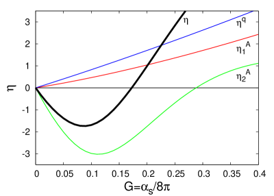
Figure 1: Anomalous dimension $\eta$ as a function of $G=\frac{\alpha_{s}}{8\pi}$ for $4d$ $SU(N_{\text{c}}=3)$ theory with $N_{\text{f}}=3$ massless quark flavors at vanishing temperature. The gluonic parts $\eta_{1}^{A},\eta_{2}^{A}$ and the quark part $\eta^{\text{q}}$ contributing to the anomalous dimension $\eta$ (thick black line) are shown separately. The gluonic parts $\eta_{1}^{A}$ and $\eta_{2}^{A}$ agree with the results found in [13]. The figure shows the results from a calculation with a background field pointing into the 8-direction in color space.

We outline the resummation of $\eta$ of Eq. (26) in App. B, yielding

$$\eta=\eta_{1}^{A}+\eta_{2}^{A}+\eta^{\text{q}},$$ (28)

with gluonic parts $\eta_{1}^{A},\eta_{2}^{A}$ and the quark contribution to the gluon anomalous dimension $\eta^{\text{q}}$. Finite integral representations of these functions are given in Eqs. (B.17), (B.23), and (B.24). For pure gluodynamics, $\eta_{1}^{A}$ and $\eta_{2}^{A}$ carry the full information about the running coupling.

In Fig. 1, we show the result for the anomalous dimension $\eta$ as a function of $G=\frac{\alpha_{s}}{8\pi}$ for $N_{\text{c}}=3$ and $N_{\text{f}}=3$ in $d=4$ dimensions. For pure gluodynamics (i.e. $N_{\text{f}}=0$), we find an IR stable fixed point for vanishing temperature,

$$\alpha_{*}=[\alpha_{*,8},\alpha_{*,3}]\approx[5.7,9.7],$$ (29)

in agreement with the results found in [13]. The (theoretical) uncertainty is due to the fact that we have used a simple approximation for the exact color factors $\tau_{j}^{A}$ and $\tau_{j}^{\psi}$, see App. C for details. This approximation introduces an artificial dependence on the color direction of the background field. The extremal cases of this dependence are given by the 3- and 8-direction in the Cartan sub-algebra, the results of which span the above interval for the IR fixed point. Even though this uncertainty is quantitatively large in the pure-glue case, it has little effect on the quantitative results for full QCD, see below.

The inclusion of light quarks yields a lower value for the infrared fixed point $\alpha_{*}$, as can be seen from Fig. 1. However, this lower fixed point will only be attained if quarks stay massless or light in the deep IR. If $\chi$SB occurs, the quarks become massive and decouple from the flow, such that the system is expected to approach the pure-glue fixed point. In any case, we can read off from Fig. 1 that, already in the symmetric regime, the inclusion of quarks leads to a smaller coupling $\alpha_{s}$ for scales $k>k_{\chi SB}$, as compared to the coupling of a pure gluonic system.

3.2 Running-coupling results

For quantitative results on the running coupling, we confine ourselves to $d=4$ dimensions and to the gauge groups SU(2) and SU(3). Of course, results for arbitrary $d>2$ and other gauge groups can straightforwardly be obtained from our general expressions in App. B.

To this end, a quantitative evaluation of the coupling flow requires the specification of the regulator shape function $r(y)$, cf. Eq. (2). In order to make simple contact with measured values of the coupling, e.g., at the $Z$ mass or the $\tau$ mass, it is advantageous to choose $r(y)$ in correspondence with a regularization scheme for which the running of the coupling is sufficiently close to the standard $\overline{\text{MS}}$ running in the perturbative domain. Here, it is important to note that already the two-loop $\beta_{g^{2}}$ coefficient depends on the regulator, owing to both the truncation as well as the mass-dependent regularization scheme. As an example, we give the two-loop $\beta_{g^{2}}$ function calculated from Eq. (22) for QCD with $N_{\text{c}}$ colors and $N_{\text{f}}$ massless quark flavors in $d=4$ dimensions:

$$\beta(g^{2}) = -{\Bigg{(}\frac{22}{3}\bar{h}_{\frac{1}{2}}^{A}N_{\text{c}}-\frac{4}{3}\bar{h}_{\frac{1}{2}}^{\psi}N_{\text{f}}\Bigg{)}\frac{g^{4}}{(4\pi)^{2}}}-\Bigg{(}\,\frac{77N_{\text{c}}^{2}\bar{h}_{\frac{1}{2}}^{A}-14N_{\text{c}}N_{\text{f}}\bar{h}_{\frac{1}{2}}^{\psi}}{3}\,\bar{g}_{\frac{1}{2}}^{A}$$

$$\qquad\quad-\frac{127\tau_{2}^{A}\bar{h}_{\frac{5}{2}}^{A}+N_{\text{f}}\tau_{2}^{\psi}\bar{h}_{\frac{5}{2}}^{\psi}}{45}\Big{(}3(N_{\text{c}}^{2}-1)(\bar{h}_{-\frac{3}{2}}^{A}-\bar{g}_{-\frac{3}{2}}^{A})+2(\bar{H}_{0}^{A}-\bar{G}_{0}^{A})\Big{)}\Bigg{)}\frac{g^{6}}{(4\pi)^{4}}+\dots$$

The moments $\bar{g}_{j}^{A/\psi}$,$\bar{h}_{j}^{A/\psi}$, $\bar{G}_{j}^{A}$ and $\bar{H}_{j}^{A}$ are defined in App. A. They specify the regulator dependence of the loop terms and depend on $\frac{T}{k}$, as is visualized in Fig. 2.

Figure 2: Thermal moments as a function of $\frac{T}{k}$ for the exponential regulator. The moments $h_{i}^{A}$ as well as $h_{i}^{\psi}$ are finite in the limit $\frac{T}{k}\rightarrow 0$. The gluonic thermal moments $h_{i}^{A}$ grow linearly for increasing $\frac{T}{k}$ due to the presence of a soft Matsubara mode, whereas the fermionic thermal moments $h_{i}^{\psi}$ are exponentially supressed for $\frac{T}{k}\rightarrow\infty$.

We observe that even the one-loop coefficient is regulator dependent at finite temperature, but universal and exact at zero temperature, as it should. The latter holds, since $\bar{g}_{\frac{1}{2}}^{A/\psi}(\frac{T}{k}=0)=1$ and $\bar{h}_{\frac{1}{2}}^{A/\psi}(\frac{T}{k}=0)=1$ for all admissible regulators. Using the exponential regulator, we find $\bar{h}_{-\frac{3}{2}}^{A}(\frac{T}{k}=0)=2\zeta(3)$, $\bar{g}_{-\frac{3}{2}}^{A}(\frac{T}{k}=0)=1$, $\bar{h}_{\frac{5}{2}}^{A/\psi}(\frac{T}{k}=0)=\frac{1}{6}$, $\bar{G}_{0}^{A}(\frac{T}{k}=0)=\frac{1}{2}$ and $\bar{H}_{0}^{A}(\frac{T}{k}=0)=\zeta(3)$ for the moments at zero temperature. Using the color factors $\tau_{2}^{A}$ and $\tau_{2}^{\psi}$ from App. C, we compare our result to the perturbative two-loop result,

$$\beta_{pert.}(g^{2})=-{\Bigg{(}\frac{22}{3}N_{\text{c}}-\frac{4}{3}N_{\text{f}}\Bigg{)}\frac{g^{4}}{(4\pi)^{2}}}-\Bigg{(}\frac{68N_{\text{c}}^{3}+6N_{\text{f}}-26N_{\text{c}}^{2}N_{\text{f}}}{3N_{\text{c}}}\Bigg{)}\frac{g^{6}}{(4\pi)^{4}}+\dots\,,$$ (31)

and find good agreement to within 99% for the two-loop coefficient for SU(2) and 95% for SU(3) pure gauge theory. Beside this compatibility with the standard $\overline{\mathrm{MS}}$ running the exponential regulator is technically and numerically convenient.

The perturbative quality of the regulator is mandatory for a reliable estimate of absolute, i.e., dimensionful, scales of the final results. The present choice enables us to fix the running coupling to experimental input: as initial condition, we use the measured value of the coupling at the $\tau$ mass scale [38], $\alpha_{\mathrm{s}}=0.322$, which by RG evolution agrees with the world average of $\alpha_{\mathrm{s}}$ at the $Z$ mass scale. We stress that no other parameter or scale is used as an input.

The global behavior of the running coupling can be characterized in simple terms. Let us first concentrate on pure gluodynamics, setting $N_{\text{f}}\to 0$ for a moment. At zero temperature, we rediscover the results of [13], exhibiting a standard perturbative behavior in the UV. In the IR, the coupling increases and approaches a stable fixed point $g^{2}_{\ast}$ which is induced by a second zero of the $\beta_{g^{2}}$ function, see Fig. 3. The appearance of an IR fixed point in Yang-Mills theories is a well-investigated phenomenon also in the Landau gauge [39]. Here, the IR fixed point is a consequence of a tight link between the fully dressed gluon and ghost propagators at low momenta which is visible in a vertex expansion [40]. Most interestingly, this behavior is in accordance with the Kugo-Ojima and Gribov-Zwanziger confinement scenarios [41]. Even though the relation between the Landau-gauge and the background-gauge IR fixed point is not immediate, it is reassuring that the definition of the running coupling in both frameworks rests on a nonrenormalization property that arises from gauge invariance [42, 16]. Within the present mass-dependent RG scheme, the appearance of an IR fixed point is moreover compatible with the existence of a mass gap: once the scale $k$ has dropped below the lowest physical state in the spectrum, the running of physically relevant couplings should freeze out, since no fluctuations are left to drive any further RG flow. Finally, IR fixed-point scenarios have successfully been applied also in phenomenological studies [43, 44, 45, 46, 47, 48].

At finite temperature, the small-coupling UV behavior remains unaffected for scales $k\gg T$ and agrees with the zero-temperature perturbative running as expected. Towards lower scales, the coupling increases until it develops a maximum near $k\sim T$. Below, the coupling decreases according to a powerlaw $g^{2}\sim k/T$, see Fig. 3. This behavior has a simple explanation: the wavelength of fluctuations with momenta $p^{2}<T^{2}$ is larger than the extent of the compactified Euclidean time direction. Hence, these modes become effectively 3-dimensional and their limiting behavior is governed by the spatial 3$d$ Yang-Mills theory. As a nontrivial result, we observe the existence of a non-Gaußian IR fixed point also in the reduced 3$d$ theory, see also Sec. 3.3. By virtue of a straightforward matching between the 4$d$ and 3$d$ coupling, the observed powerlaw for the 4$d$ coupling is a direct consequence of the strong-coupling 3$d$ IR behavior, $g^{2}(k\ll T)\sim g^{2}_{3d,\ast}\,k/T$. Again, the observation of an IR fixed point in the 3$d$ theory agrees with recent results in the Landau gauge [49].

Figure 3: Running $\mathrm{SU}(3)$ Yang-Mills coupling $\alpha_{\scriptscriptstyle{\mathrm{YM}}}(k,T)$ as a function of $k$ for $T=0,100,500\,\mathrm{MeV}$ compared to the one-loop running for vanishing temperature.

The 3$d$ IR fixed point and the perturbative UV behavior already qualitatively determine the momentum asymptotics of the running coupling. Phenomenologically, the behavior of the coupling in the transition region near its maximum value is most important, which is quantitatively provided by the full 4$d$ finite-temperature flow equation. In addition to the shift of the position of the maximum with temperature, we observe a decrease of the maximum itself for increasing temperature. On average, the 4$d$ coupling gets weaker for higher temperature, in agreement with naive expectations. We emphasize, however, that this behavior results from a nontrivial interplay of various nonperturbative contributions.

Figure 4: Running $\mathrm{SU}(3)$ coupling $\alpha_{s}(k,T)$ as a function of $k$ for $T=100\,\mathrm{MeV}$ for different number of quark flavors $N_{\text{f}}=0,1,2,\dots,10$ (from top to bottom). For $k\ll T$, the coupling shows universal behavior, owing to the attraction of the pure-glue IR fixed point.

Now, we turn to the effect of a finite number $N_{\text{f}}$ of massless quark flavors. In Fig. 4, we show the running coupling $\alpha_{s}$ as a function of $k$ for $T=100\leavevmode\nobreak\ \mathrm{MeV}$ and for $N_{\text{f}}=0,\dots,10$. At high scales $k\gg T$, the running of the coupling agrees with the zero-temperature running in the presence of $N_{\text{f}}$ massless quark flavors. Towards lower scales, the coupling increases less strongly than the coupling of the corresponding SU(3) Yang-Mills theory, due to fermionic screening. At a scale $k\sim T$, the coupling reaches its maximum. Below this scale, the quarks decouple from the flow, since they only have hard Matsubara modes and, hence, the coupling universally approaches the result for pure Yang-Mills theory. Furthermore, we observe that, for an increasing number of quark flavors, the maximum of the coupling becomes smaller and moves towards lower scales. Both effects are due to the fact that the anomalous dimension $\eta$ becomes smaller for an increasing number of quark flavors.

Again, we stress that the results for the coupling with dynamical quarks have not yet accounted for $\chi$SB, where the quarks become massive and decouple from the flow. This will be discussed in the following sections. For temperatures or flavor numbers larger than the corresponding critical value for $\chi$SB, our results so far should be trustworthy on all scales.

3.3 Dimensionally reduced high-temperature limit

As discussed above, the running coupling for scales much lower than the temperature, $k\ll T$, is governed by the IR fixed point of the 3-dimensional theory. More quantitatively, we observe that the flow of the coupling is completely determined by $\eta_{1}^{A}$ for $\frac{T}{k}\gg 1$; the quark contributions decouple from the flow in this limit, since they do not have a soft Matsubara mode. Therefore, we find an IR fixed point at finite temperature for the 4$d$ theory at $g^{2}=0$. In the limit $\frac{T}{k}\gg 1$, the anomalous dimension Eq. (28) is given by

$$\eta(T\gg k)\approx\eta_{1}^{A}(T\gg k)=:\eta_{1}^{\infty}(g^{2},\textstyle{\frac{T}{k}})=\bar{\gamma}_{3d}\,\left(\textstyle{\frac{T}{k}}\,g^{2}\right)^{\frac{5}{4}},$$ (32)

where $\bar{\gamma}_{3d}$ is a number which depends on $N_{\text{c}}$:

$$\bar{\gamma}_{3d}=\frac{32\zeta(\frac{5}{2})(1-2\sqrt{2})\Gamma(\frac{9}{4})\Gamma(\frac{5}{4}+z_{4}^{\infty})\sqrt[4]{{c}_{1}^{\infty}}}{(4\pi)^{4}\Gamma(\frac{3}{2})\Gamma(z_{4}^{\infty}+1)}N_{\text{c}}.$$ (33)

We refer to App. B for the definition of the constants $z_{4}^{\infty}$ and ${c}_{1}^{\infty}$. In the high-temperature limit, we can solve the differential equation (14) for $g^{2}$ analytically,

$$g^{2}\Big{|}_{\frac{T}{k}\gg 1}=:g_{\infty}^{2}({\textstyle{\frac{k}{T}}})=\frac{1}{(\bar{\gamma}_{3d}(\frac{T}{k})^{\frac{5}{4}}-\mathrm{{const.}})^{\frac{4}{5}}}\,\approx\,\bar{\gamma}_{3d}^{-\frac{4}{5}}\,{\frac{k}{T}}+\mathcal{O}((\textstyle{\frac{k}{T}})^{2}).$$ (34)

The RHS explains the shape of the running coupling for small $k/T$ in Fig. 3. The factor $\bar{\gamma}_{3d}^{-\frac{4}{5}}$ is the fixed point value of the dimensionless 3$d$ coupling ${g}_{3d}^{2}$, as can be seen from its relation to the dimensionless coupling $g^{2}$ in four dimensions:

$$g_{3d}^{2}:=\frac{T}{k}\,g^{2}\quad\rightarrow g^{2}=\frac{k}{T}\,{g}_{3d}^{2}\,.$$ (35)

Comparing the right-hand side of Eq. (34) and (35), we find that the fixed point for $N_{\text{c}}=3$ in three dimensions is given by:

$$\alpha_{*}^{3d}\equiv\frac{{g}_{3d,*}^{2}}{4\pi}=[\alpha_{*,8}^{3d},\alpha_{*,3}^{3d}]\approx[2.70,2.77]$$ (36)

Again, the uncertainty arises from our ignorance of the exact color factors $\tau_{m}^{A}$, see App. B and App. C.

On the other hand, the fixed point of the 3d theory is determined by the zero of the corresponding $\beta$ function. In fact, $\eta_{1}^{\infty}(g^{2},\textstyle{\frac{T}{k}})$ is identical to the 3d anomalous dimension $\eta_{3d}({g}_{3d}^{2})$, as can be deduced from the pure $3d$ theory, and we obtain

$$\partial_{t}(\textstyle{\frac{T}{k}}g^{2})\equiv\partial_{t}{g}_{3d}^{2}=(\eta_{3d}({g}_{3d}^{2})-1){g}_{3d}^{2},$$ (37)

as suggested by Eq. (14). Since $\eta_{3d}$ is a monotonously increasing function, we find a $3d$ IR fixed point for ${g}_{3d,*}^{2}=\bar{\gamma}_{3d}^{-\frac{4}{5}}$ which coincides with the result above.

4 Chiral quark dynamics

Dynamical quarks influence the QCD flow by two qualitatively different mechanisms. First, quark fluctuations directly modify the running coupling as already discussed above; the nonperturbative contribution in the form of $\eta^{\text{q}}$ in Eq. (28) accounts for the screening nature of fermionic fluctuations, generalizing the tendency that is already visible in perturbation theory. Second, gluon exchange between quarks induces quark self-interactions which can become relevant in the strongly coupled IR. Both the quark and the gluon sector feed back onto each other in an involved nonlinear fashion. In general, these nonlinearities have to be taken into account and are provided by the flow equation. However, we will argue that some intricate nonlinearities drop out or are negligible for locating the chiral phase boundary in a first approximation.

Working solely in $d=4$ from here on, let us now specify the last part of our truncation: the effective action of quark self-interactions $\Gamma_{k}^{\text{q-int}}[\bar{\psi},\psi]$, introduced in Eq. (17). In a consistent and systematic operator expansion, the lowest nontrivial order is given by [52]

$$\Gamma_{k} = \int_{x}\frac{1}{2}\Big{[}\bar{\lambda}_{-}(\text{V--A})+\bar{\lambda}_{+}(\text{V+A})+\bar{\lambda}_{\sigma}(\text{S--P})+\bar{\lambda}_{\text{VA}}[2(\text{V--A})^{\text{adj}}\!+({1}/{N_{\text{c}}})(\text{V--A})]\Big{]}.$$ (38)

The four-fermion interactions occurring here have been classified according to their color and flavor structure. Color and flavor singlets are

$$(\text{V--A}) = (\bar{\psi}\gamma_{\mu}\psi)^{2}+(\bar{\psi}\gamma_{\mu}\gamma_{5}\psi)^{2},$$ (39)

$$(\text{V+A}) = (\bar{\psi}\gamma_{\mu}\psi)^{2}-(\bar{\psi}\gamma_{\mu}\gamma_{5}\psi)^{2},$$ (40)

where (fundamental) color ($i,j,\dots$) and flavor ($\chi,\xi,\dots$) indices are contracted pairwise, e.g., $(\bar{\psi}\psi)\equiv(\bar{\psi}_{i}^{\chi}\psi_{i}^{\chi})$. The remaining operators have non-singlet color or flavor structure,

$$(\text{S--P}) = (\bar{\psi}^{\chi}\psi^{\xi})^{2}-(\bar{\psi}^{\chi}\gamma_{5}\psi^{\xi})^{2}\equiv(\bar{\psi}_{i}^{\chi}\psi_{i}^{\xi})^{2}-(\bar{\psi}_{i}^{\chi}\gamma_{5}\psi_{i}^{\xi})^{2},$$

$$(\text{V--A})^{\text{adj}} = (\bar{\psi}\gamma_{\mu}T^{a}\psi)^{2}+(\bar{\psi}\gamma_{\mu}\gamma_{5}T^{a}\psi)^{2},$$ (41)

where $(\bar{\psi}^{\chi}\psi^{\xi})^{2}\equiv\bar{\psi}^{\chi}\psi^{\xi}\bar{\psi}^{\xi}\psi^{\chi}$, etc., and $(T^{a})_{ij}$ denotes the generators of the gauge group in the fundamental representation. The set of fermionic self-interactions introduced in Eq. (38) forms a complete basis. Any other pointlike four-fermion interaction which is invariant under $\textrm{SU}(N_{\text{c}})$ gauge symmetry and $\textrm{SU}(N_{\text{f}})_{\textrm{L}}\times\textrm{SU}(N_{\text{f}})_{\textrm{R}}$ flavor symmetry is reducible by means of Fierz transformations. U${}_{\text{A}}(1)$-violating interactions are neglected, since we expect them to become relevant only inside the $\chi$SB regime or for small $N_{\text{f}}$; since the lowest-order U${}_{\text{A}}$(1)-violating term schematically is $\sim(\bar{\psi}\psi)^{N_{\text{f}}}$, larger $N_{\text{f}}$ correspond to larger RG “irrelevance” by naive power-counting. For $N_{\text{f}}=1$, such a term is, of course, important, since it provides for a direct fermion mass term; in this case, the chiral transition is expected to be a crossover. Dropping the U${}_{\text{A}}(1)$-violating interactions, we thus confine ourselves to $N_{\text{f}}\geq 2$.

We emphasize that the $\bar{\lambda}$’s are not considered as independent external parameters as, e.g., in the Nambu–Jona-Lasinio model. More precisely, we impose the boundary condition $\bar{\lambda}_{i}\to 0$ for $k\to\Lambda\to\infty$ which guarantees that the $\bar{\lambda}$’s at $k<\Lambda$ are solely generated by quark-gluon dynamics, e.g., by 1PI “box” diagrams with 2-gluon exchange.

As a severe approximation, we drop any nontrivial momentum dependencies of the $\bar{\lambda}$’s and study these couplings in the point-like limit $\bar{\lambda}(|p_{i}|\ll k)$. This inhibits a study of QCD properties in the chirally broken regime, since mesons, for instance, manifest themselves as momentum singularities in the $\bar{\lambda}$’s. Nevertheless, the point-like truncation can be a reasonable approximation in the chirally symmetric regime; this has recently been quantitatively confirmed for the zero-temperature chiral phase transition in many-flavor QCD [50], where the regulator independence of universal quantities has been shown to hold remarkably well even in this restrictive truncation. By adopting the same system at finite $T$, we base our truncation on the assumption that quark dynamics both near the finite-$T$ phase boundary as well as near the many-flavor phase boundary [51] is driven by qualitatively similar mechanisms.

The resulting flow equations for the $\bar{\lambda}$’s are a straightforward generalization of those derived and analyzed in [52, 50] to the case of finite temperature. Introducing the dimensionless renormalized couplings

$$\lambda_{i}={k^{2}\bar{\lambda_{i}}},$$ (42)

(recall that $Z_{\psi}=1$ in our truncation), the flows of the quark interactions read

$$\partial_{t}\lambda_{-} = 2\lambda_{-}\!-4v_{4}l^{\textrm{(FB)}}_{1,1}\left[\frac{3}{N_{\text{c}}}g^{2}\lambda_{-}-3g^{2}\lambda_{\text{VA}}\right]-\frac{1}{8}v_{4}l^{\textrm{(FB)}}_{1,2}\left[\frac{12+9N_{\text{c}}^{2}}{N_{\text{c}}^{2}}g^{4}\right]$$

$$\!\!-8v_{4}l_{1}^{\text{(F)}}\Big{\{}-N_{\text{f}}N_{\text{c}}(\lambda_{-}^{2}+\lambda_{+}^{2})+\lambda_{-}^{2}-2(N_{\text{c}}+N_{\text{f}})\lambda_{-}\lambda_{\text{VA}}+N_{\text{f}}\lambda_{+}\lambda_{\sigma}+2\lambda_{\text{VA}}^{2}\Big{\}},$$

$$\!\partial_{t}\lambda_{+} = 2\lambda_{+}\!-4v_{4}l^{\textrm{(FB)}}_{1,1}\left[-\frac{3}{N_{\text{c}}}g^{2}\lambda_{+}\right]-\frac{1}{8}v_{4}l^{\textrm{(FB)}}_{1,2}\left[-\frac{12+3N_{\text{c}}^{2}}{N_{\text{c}}^{2}}g^{4}\right]$$

$$-8v_{4}l_{1}^{\text{(F)}}\Big{\{}-3\lambda_{+}^{2}-2N_{\text{c}}N_{\text{f}}\lambda_{-}\lambda_{+}-2\lambda_{+}(\lambda_{-}+(N_{\text{c}}+N_{\text{f}})\lambda_{\text{VA}})+N_{\text{f}}\lambda_{-}\lambda_{\sigma}$$

$$\!\!\quad\quad\quad\qquad+\lambda_{\text{VA}}\lambda_{\sigma}+{\scriptstyle\frac{1}{4}}\lambda_{\sigma}{}^{2}\Big{\}},$$

$$\partial_{t}\lambda_{\sigma} = 2\lambda_{\sigma}\!-4v_{4}l^{\textrm{(FB)}}_{1,1}\left[6C_{2}(N_{\text{c}})\,g^{2}\lambda_{\sigma}-6g^{2}\lambda_{+}\right]-\frac{1}{4}v_{4}l^{\textrm{(FB)}}_{1,2}\Big{[}-\frac{24-9N_{\text{c}}^{2}}{N_{\text{c}}}\,g^{4}\Big{]}$$

$$-8v_{4}l_{1}^{\text{(F)}}\Big{\{}2N_{\text{c}}\lambda_{\sigma}^{2}\!-\!2\lambda_{-}\lambda_{\sigma}\!-2N_{\text{f}}\lambda_{\sigma}\lambda_{\text{VA}}\!\!-\!6\lambda_{+}\lambda_{\sigma}\!\Big{\}},$$

$$\partial_{t}\lambda_{\text{VA}} = 2\lambda_{\text{VA}}\!-4v_{4}l^{\textrm{(FB)}}_{1,1}\left[\frac{3}{N_{\text{c}}}g^{2}\lambda_{\text{VA}}-3g^{2}\lambda_{-}\right]-\frac{1}{8}v_{4}l^{\textrm{(FB)}}_{1,2}\left[-\frac{24-3N_{\text{c}}^{2}}{N_{\text{c}}}g^{4}\right]$$

$$-8v_{4}l_{1}^{\text{(F)}}\!\Big{\{}\!-\!(N_{\text{c}}+N_{\text{f}})\lambda_{\text{VA}}^{2}\!+4\lambda_{-}\lambda_{\text{VA}}\!-{\scriptstyle\frac{1}{4}}N_{\text{f}}\lambda_{\sigma}^{2}\Big{\}}.$$

Here, $C_{2}(N_{\text{c}})=(N_{\text{c}}^{2}-1)/(2N_{\text{c}})$ is a Casimir operator of the gauge group, and $v_{4}=1/(32\pi^{2})$. For better readability, we have written all gauge-coupling-dependent terms in square brackets, whereas fermionic self-interactions are grouped inside braces. The threshold functions $l_{1}^{\text{(F)}},l^{\textrm{(FB)}}_{1,2},l^{\textrm{(FB)}}_{1,1}$ depend on the details of the regularization, see App. A; for zero quark mass and vanishing temperature, these functions reduce to simple positive numbers, see, e.g., Eqs. (A.26) and (A.29). For quark masses and temperature becoming larger than the regulator scale $k$, these functions approach zero, which reflects the decoupling of massive modes from the flow.

Within this set of degrees of freedom, a simple picture for the chiral dynamics arises: for vanishing gauge coupling, the flow is solved by vanishing $\lambda_{i}$’s, which defines the Gaußian fixed point. This fixed point is IR attractive, implying that these self-interactions are RG irrelevant for sufficiently small bare couplings, as they should. At weak gauge coupling, the RG flow generates quark self-interactions of order $\lambda\sim g^{4}$, as expected for a perturbative 1PI scattering amplitude. The back-reaction of these self-interactions on the total RG flow is negligible at weak coupling. If the gauge coupling in the IR remains smaller than a critical value $g<g_{\text{cr}}$, the self-interactions remain bounded, approaching fixed points in the IR. These fixed points can simply be viewed as order-$g^{4}$ shifted versions of the Gaußian fixed point, being modified by the gauge dynamics. At these fixed points, the fermionic subsystem remains in the chirally invariant phase which is indeed realized at high temperature.

Figure 5: Sketch of a typical $\beta$ function for the fermionic self-interactions $\lambda_{i}$: at zero gauge coupling, $g=0$ (upper solid curve), the Gaußian fixed point $\lambda_{i}=0$ is IR attractive. For small $g\gtrsim 0$ (middle/blue solid curve), the fixed-point positions are shifted on the order of $g^{4}$. For gauge couplings larger than the critical coupling $g>g_{\text{cr}}$ (lower/green solid curve), no fixed points remain and the self-interactions quickly grow large, signaling $\chi$SB. For increasing temperature, the parabolas become broader and higher, owing to thermal fermion masses; this is indicated by the dashed/red line.

If the gauge coupling increases beyond the critical coupling $g>g_{\text{cr}}$, the above-mentioned IR fixed points are destabilized and the quark self-interactions become critical. This can be visualized by the fact that $\partial_{t}\lambda_{i}$ as a function of $\lambda_{i}$ is an everted parabola, see Fig. 5; for $g=g_{\text{cr}}$, the parabola is pushed below the $\lambda_{i}$ axis, such that the (shifted) Gaußian fixed point annihilates with the second zero of the parabola. In this case, the gauge-fluctuation-induced $\bar{\lambda}$’s have become strong enough to contribute as relevant operators to the RG flow. These couplings now increase rapidly, approaching a divergence at a finite scale $k=k_{\text{$\chi$SB}}$. In fact, this seeming Landau-pole behavior indicates $\chi$SB and, more specifically, the formation of chiral condensates. This is because the $\bar{\lambda}$’s are proportional to the inverse mass parameter of a Ginzburg-Landau effective potential for the order parameter in a (partially) bosonized formulation, $\bar{\lambda}\sim 1/m^{2}$. Thus, the scale at which the self-interactions formally diverge in our truncation is a good measure for the scale $k_{\text{$\chi$SB}}$ where the effective potential for the chiral order parameter becomes flat and is about to develop a nonzero vacuum expectation value.

Whether or not chiral symmetry is preserved by the ground state therefore depends on the coupling strength of the system, more specifically, the value of the gauge coupling $g$ relative to the critical coupling $g_{\text{cr}}$ which is required to trigger $\chi$SB. Incidentally, the critical coupling $g_{\text{cr}}$ itself can be determined by algebraically solving the fixed-point equations $\partial_{t}\lambda_{i}(\lambda_{\ast})=0$ for that value of the coupling, $g=g_{\text{cr}}$, where the shifted Gaußian fixed point is annihilated. For instance, at zero temperature, the SU(3) critical coupling for the quarks system is $\alpha_{\text{cr}}\equiv g^{2}_{\text{cr}}/(4\pi)\simeq 0.8$ [53], being only weakly dependent on the number of flavors [50]. Since the IR fixed point for the gauge coupling is much larger $\alpha_{\ast}>\alpha_{\text{cr}}$ (for not too many massless flavors), the QCD vacuum is characterized by $\chi$SB. The same qualitative observations have already been made in [54] in a similar though smaller truncation. The existence of such a critical coupling also is a well-studied phenomenon in Dyson-Schwinger equations [55].

As soon as the the quark sector approaches criticality, also its back-reaction onto the gluon sector becomes sizable. Here, a subtlety of the present formalism becomes important: identifying the fluctuation field with the background field under the flow, our approximation generally does not distinguish between the flow of the background-field coupling and that of the fluctuation-field coupling. In our truncation, differences arise from the quark self-interactions. Whereas the running of the background-field coupling is always given by Eq. (14), the quark self-interactions can contribute directly to the running of the fluctuation-field coupling in the form of a “vertex correction” to the quark-gluon vertex. Since the fluctuation-field coupling is responsible for inducing quark self-interactions, this difference may become important. In [52], the relevant terms have been derived with the aid of a regulator-dependent Ward-Takahashi identity. The result hence implements an important gauge constraint, leading us to

$$\partial_{t}g^{2} = \eta\,g^{2}-4v_{4}l_{1}^{\text{(F)}}\,\frac{g^{2}}{1-2v_{4}l_{1}^{\text{(F)}}\sum c_{i}\lambda_{i}}\,\partial_{t}\sum c_{i}\lambda_{i},$$

$$c_{\sigma}=1+N_{\text{f}},\,\,c_{+}=0,\,\,c_{-}=-2,\,\,c_{\textrm{VA}}=-2N_{\text{f}},$$

with $\eta$ provided by Eq. (28) in our approximation. In principle, the approach to $\chi$SB can now be studied by solving the coupled system of Eqs. (4), and (4)-(4). However, a simpler and, for our purposes, sufficient estimate is provided by the following argument: if the system ends up in the chirally symmetric phase, the $\lambda_{i}$’s always stay close to the shifted Gaußian fixed point discussed above; apart from a slight variation of this fixed-point position with increasing $g^{2}$, the $\partial_{t}\lambda_{i}$ flow is small and vanishes in the IR, $\partial_{t}\lambda_{i}\to 0$. Therefore, the additional terms in Eq. (4) are negligible for all $k$ and drop out in the IR. As a result, the behavior of the running coupling in the chirally symmetric phase is basically determined by $\eta$ alone, as discussed in the preceding section. In other words, the difference between the fluctuation-field coupling and the background-field coupling automatically switches off in the deep IR in the symmetric phase in our truncation.

Therefore, if the coupling as predicted by $\beta_{g^{2}}\simeq\eta g^{2}$ alone never increases beyond the critical value $g^{2}_{\text{cr}}$ for any $k$, the system is in the chirally symmetric phase. In this case, it suffices to solve the $g^{2}$ flow and compare it with $g^{2}_{\text{cr}}$ which can be deduced from a purely algebraic solution of the fixed-point equations, $\partial_{t}\lambda_{i}(\lambda_{\ast})=0$.

If the coupling as predicted by $\beta_{g^{2}}\simeq\eta g^{2}$ alone approaches $g_{\text{cr}}$ for some finite scale $k_{\text{cr}}$, the quark sector becomes critical and all couplings start to flow rapidly. To the present level of accuracy, this serves as an indication for $\chi$SB. Of course, if the gauge coupling dropped quickly for decreasing $k$, the quark sector could, in principle, become subcritical again. However, this might happen only for a marginal range of $g^{2}\simeq g^{2}_{\text{cr}}$ if at all. For even larger gauge coupling, the flow towards $\chi$SB is unavoidable.

Inside the $\chi$SB regime, also the induced quark masses back-react onto the gluonic flow in the form of a decoupling of the quark fluctuations, i.e., $\eta^{\text{q}}$ in Eq. (28) approaches zero. However, the present truncation does not allow to explore the properties of the $\chi$SB sector; for this, the introduction of effective mesonic degrees of freedom along the lines of [53, 56] is most useful and will be employed in future work.

5 Chiral phase transition

Let us now discuss our results for the chiral phase transition in the framework presented so far. As elucidated in the previous section, the breaking of chiral-symmetry is triggered if the gauge coupling $g^{2}$ increases beyond $g^{2}_{\text{cr}}$, signaling criticality of the quark sector. We study the dependence of the chiral symmetry status on two parameters: temperature $T$ and number of (massless) flavors $N_{\text{f}}$. As already discussed in Sect. 3, the increase of the running coupling in the IR is weakened on average for both larger $T$ and larger $N_{\text{f}}$. In addition, also $g_{\text{cr}}$ depends on $T$ and $N_{\text{f}}$, even though the $N_{\text{f}}$ dependence is rather weak.

The $T$ dependence of $g_{\text{cr}}$ has a physical interpretation: at finite $T$, all quark modes acquire thermal masses which leads to a quark decoupling for $k\lesssim T$. Hence, stronger interactions are required to excite critical quark dynamics. Technically, this $T/k$ dependence is a direct consequence of the $T/k$ dependence of the threshold functions $l_{1}^{\text{(F)}},l^{\textrm{(FB)}}_{1,2},l^{\textrm{(FB)}}_{1,1}$ in Eqs.  (4) - (4), see App. A for their definition. Since the threshold functions decrease with increasing temperature, the $\lambda_{i}$ parabolas visualized in Fig. 5 become broader with a higher maximum; hence, the annihilation of the Gaußian fixed point by pushing the parabola below the $\lambda_{i}$ axis requires a larger $g_{\text{cr}}$.

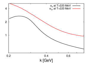
Figure 6: Running QCD coupling $\alpha_{\mathrm{s}}(k,T)$ for $N_{\text{f}}=3$ massless quark flavors and $N_{\text{c}}=3$ colors and the critical value of the running coupling $\alpha_{\mathrm{cr}}(k,T)$ as a function of $k$ for $T=130\,\mathrm{MeV}$ (left panel) and $T=220\,\mathrm{MeV}$ (right panel). The existence of the $(\alpha_{\mathrm{s}},\alpha_{\mathrm{cr}})$ intersection point in the left panel indicates that the $\chi$SB quark dynamics can become critical for $T=130\,\mathrm{MeV}$.

At zero temperature and for small $N_{\text{f}}$, the IR fixed point of the running coupling is far larger than $g^{2}_{\text{cr}}$, hence the QCD vacuum is in the $\chi$SB phase. For increasing $T$, the temperature dependence of the coupling and that of $g^{2}_{\text{cr}}$ compete with each other. This is illustrated in Fig. 6 where we show the running coupling $\alpha_{\mathrm{s}}\equiv\frac{g^{2}}{4\pi}$ and its critical value $\alpha_{\mathrm{cr}}\equiv\frac{g_{cr}^{2}}{4\pi}$ for $T=130\,\mathrm{MeV}$ and $T=220\,\mathrm{MeV}$ as a function of the regulator scale $k$. The intersection point $k_{\text{cr}}$ between both marks the scale where the quark dynamics becomes critical. Below the scale $k_{\text{cr}}$, the system runs quickly into the $\chi$SB regime. We estimate the critical temperature $T_{\text{cr}}$ as the lowest temperature for which no intersection point between $\alpha_{\mathrm{s}}$ and $\alpha_{\mathrm{cr}}$ occurs. We find

$$T_{\mathrm{cr}} \approx 186\pm 33\,\mathrm{MeV\quad for\quad}N_{\text{f}}=2,$$

$$T_{\mathrm{cr}} \approx 161\pm 31\,\mathrm{MeV\quad for\quad}N_{\text{f}}=3,$$ (48)

for massless quark flavors in good agreement with lattice simulations [57]. The errors arise from the experimental uncertainties on $\alpha_{\mathrm{s}}$ [38]. The theoretical error owing to the color-factor uncertainty turns out to be subdominant by far, see Fig. 7. Dimensionless observable ratios are less contaminated by this uncertainty of $\alpha_{\text{s}}$. For instance, the relative difference for $T_{\text{cr}}$ for $N_{\text{f}}=2$ and 3 flavors is

$$\Delta:=\frac{T_{\text{cr}}^{N_{\text{f}}=2}-T_{\text{cr}}^{N_{\text{f}}=3}}{(T_{\text{cr}}^{N_{\text{f}}=2}+T_{\text{cr}}^{N_{\text{f}}=3})/2}=0.144\genfrac{}{}{0.0pt}{}{+0.018}{-0.013},$$ (49)

in reasonable agreement with the lattice value of $\sim 0.12$ [57].

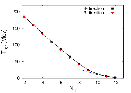
Figure 7: Chiral-phase-transition temperature $T_{\text{cr}}$ versus the number of massless quark flavors $N_{\text{f}}$ for $N_{\text{f}}\geq 2$. The flattening at $N_{\text{f}}\gtrsim 10$ is a consequence of the IR fixed-point structure. The dotted line depicts the analytic estimate near $N_{\text{f}}^{\text{cr}}$ which follows from the fixed-point scenario (cf. Eq. (55) below). Squares and triangles correspond to calculations with a background field in the 8- and 3-direction of the Cartan, respectively. The theoretical uncertainty which is given by the difference between both is obviously negligible in full QCD.

For the case of many massless quark flavors $N_{\text{f}}$, the critical temperature is plotted in Fig. 7. We observe an almost linear decrease of the critical temperature for increasing $N_{\text{f}}$ with a slope of $\Delta T_{\mathrm{cr}}=T(N_{\text{f}})-T(N_{\text{f}}+1)\approx 25\,\mathrm{MeV}$. In addition, we find a critical number of quark flavors, $N_{\text{f}}^{\mathrm{cr}}\simeq 12.9$, above which no chiral phase transition occurs. This result for $N_{\text{f}}^{\mathrm{cr}}$ agrees with other studies based on the 2-loop $\beta$ function [51]. However, the precise value of $N_{\text{f}}^{\mathrm{cr}}$ has to be taken with care: for instance, in a perturbative framework, $N_{\text{f}}^{\mathrm{cr}}$ is sensitive to the 3-loop coefficient which can bring $N_{\text{f}}^{\text{cr}}$ down to $N_{\text{f}}^{\text{cr}}\simeq 10$ [50]. In our nonperturbative approach, the truncation error can induce similar uncertainties; in fact, it is reassuring that our prediction for $N_{\text{f}}^{\text{cr}}$ lies in the same ball park as the perturbative estimates, even though the details of the corresponding $\beta_{g^{2}}$ are very different. This suggests that our truncation error for $N_{\text{f}}^{\text{cr}}$ is also of order $\mathcal{O}(1)$. We expect that a more reliable estimate can be obtained even within our truncation by a regulator [58, 15].

A remarkable feature of the $T,N_{\text{f}}$ phase diagram of Fig. 7 is the shape of the phase boundary, in particular, the flattening near $N_{\text{f}}^{\text{cr}}$. In fact, this shape can be understood analytically, revealing a direct connection between two universal quantities: the phase boundary and the IR critical exponent of the running coupling.

Before we outline the argument in detail, let us start with an important caveat: varying $N_{\text{f}}$ unlike varying $T$ corresponds to an unphysical deformation of a physical system. Whereas the deformation itself is, of course, unambiguously defined, the comparison of the physical theory with the deformed theory (or between two deformed theories) is not unique. A meaningful comparison requires to identify one parameter or one scale in both theories. In our case, we always keep the running coupling at the $\tau$ mass scale fixed to $\alpha(m_{\tau})=0.322$. Obviously, the couplings in the two theories are different on all other scales, as are generally all dimensionful quantities such as $\Lambda_{\text{QCD}}$. There is, of course, no generic choice for fixing the corresponding theories relative to each other. Nevertheless, we believe that our choice is particularly useful, since the $\tau$ mass scale is close to the transition between perturbative and nonperturbative regimes. In this sense, a meaningful comparison between the theories can be made in both regimes, without being too much afflicted by the choice of the fixing condition.

Let us now study the shape of the phase boundary for small $N_{\text{f}}$. Once the coupling is fixed to $\alpha(m_{\tau})=0.322$, no free parameter is left. As a crude approximation, the mass scale of all dimensionful IR observables such as the critical temperature $T_{\text{cr}}$ is set by the scale $k_{\text{co}}$ where the running gauge coupling undergoes the crossover from small to nonperturbatively large couplings (for instance, one can define the crossover scale $k_{\text{co}}$ from the inflection point of the running coupling in Fig. 3). As an even cruder estimate, let us approximate $k_{\text{co}}$ by the position of the Landau pole of the perturbative one-loop running coupling. The latter can be derived from the one-loop relation

$$\frac{1}{\alpha(k)}=\frac{1}{\alpha(m_{\tau})}+4\pi b_{0}\ln\frac{k}{m_{\tau}},\quad b_{0}=\frac{1}{8\pi^{2}}\left(\frac{11}{3}N_{\text{c}}-\frac{2}{3}N_{\text{f}}\right).$$ (50)

Defining $k_{\text{co}}$ by the Landau-pole scale, $1/\alpha(k_{\text{co}})=0$, and estimating the order of the critical temperature by $T_{\text{cr}}\sim k_{\text{co}}$, we obtain

$$T_{\text{cr}}\sim m_{\tau}\,\mathrm{e}^{-\frac{1}{4\pi b_{0}\alpha(m_{\tau})}}\simeq m_{\tau}\,\mathrm{e}^{-\frac{6\pi}{11N_{\text{c}}\alpha(m_{\tau})}}\left(1-\epsilon N_{\text{f}}+\mathcal{O}((\epsilon N_{\text{f}})^{2})\right),$$ (51)

where $\epsilon=\frac{12\pi}{121N_{\text{c}}^{2}\alpha(m_{\tau})}\simeq 0.107$ for $N_{\text{c}}=3$. This simple estimate hence predicts a linear decrease of the phase boundary $T_{\text{cr}}(N_{\text{f}})$ for small $N_{\text{f}}$, as is confirmed by the full solution plotted in Fig. 7. Actually, this estimate is also quantitatively accurate, since it predicts a relative difference for $T_{\text{cr}}$ for $N_{\text{f}}$=2 and 3 flavors of $\Delta\simeq 0.146$ which is in very good agreement with the full result, given in Eq. (49). We conclude that the shape of the phase boundary for small $N_{\text{f}}$ is basically dominated by fermionic screening.

For larger $N_{\text{f}}$, the above estimate can no longer be used, because neither one-loop perturbation theory nor the $N_{\text{f}}$ expansion are justified. For values of $N_{\text{f}}$ close to the critical value $N_{\text{f}}^{\text{cr}}$, a different analytic argument can be made: here the running coupling has to come close to its maximal value in order to be strong enough to trigger $\chi$SB. The maximal value is, of course, close to the IR fixed point value $\alpha_{\ast}$ attained for $T=0$. Even though at finite $T$ the coupling is eventually governed by the $3d$ fixed point implying a linear decrease with $k$, the $\chi$SB properties will still be dictated by the maximum coupling value, which roughly corresponds to the $T=0$ fixed point. In the fixed-point regime, we can approximate the $\beta_{g^{2}}$ function by a linear expansion about the fixed-point value,

$$\beta_{g^{2}}\equiv\partial_{t}g^{2}=-\Theta\,(g^{2}-g_{\ast}^{2})+\mathcal{O}((g^{2}-g_{\ast}^{2})^{2}),$$ (52)

where the universal “critical exponent” $\Theta$ denotes the (negative) first expansion coefficient. We know that $\Theta<0$, since the fixed point is IR attractive. For vanishing temperature, we find an approximate linear dependence of $\Theta$ on $N_{\text{f}}$, cf. Tab. 1.

$N_{\text{f}}$	0	4	5	6	7	8	9	10	11	12	13
$-\Theta$	6.39	5.50	4.99	4.41	3.82	3.19	2.58	1.97	1.42	0.95	0.57

Table 1: The "critical exponent" $\Theta$ for different values of $N_{\text{f}}$ for $T=0$.

The solution of Eq. (52) for the running coupling in the fixed-point regime reads

$$g^{2}(k)=g_{\ast}^{2}-\left(\frac{k}{k_{0}}\right)^{-\Theta},$$ (53)

where the scale $k_{0}$ is implicitly defined by a suitable initial condition (to be set in the fixed-point regime) and is kept fixed in the following. It provides for all dimensionful scales in the following and is related to the initial $\tau$ mass scale by RG evolution. Our criterion for $\chi$SB to occur is that $g^{2}(k)$ should exceed $g_{\text{cr}}^{2}$ for some value of $k=k_{\text{cr}}$. We expect that this scale $k_{\text{cr}}$ is generically somewhat larger than the temperature, since for $k$ smaller than $T$ the coupling decreases again owing to the $3d$ fixed point. This allows us to ignore the $T$ dependence of the running coupling $g^{2}$ and of the critical coupling $g_{\text{cr}}$ as a rough approximation, since the $T$ dependence of the threshold functions is rather weak for $T\lesssim k$. From Eq. (53) and the condition $g^{2}(k_{\text{cr}})=g^{2}_{\text{cr}}$, we derive the estimate

$$k_{\text{cr}}\simeq k_{0}\,(g_{\ast}^{2}-g_{\text{cr}}^{2})^{-\frac{1}{\Theta}}.$$ (54)

This scale $k_{\text{cr}}$ plays the same role as the crossover scale $k_{\text{co}}$ in the small-$N_{\text{f}}$ argument given above: it sets the scale for $T_{\text{cr}}\sim k_{\text{cr}}$, with a proportionality coefficient provided by the solution of the full flow. To conclude the argument, we note that the IR fixed-point value $g_{\ast}^{2}$ roughly depends linearly on $N_{\text{f}}$, since the quark contribution to the coupling flow $\eta^{\text{q}}$ is linear in $N_{\text{f}}$. From Eq. (54), we thus find the relation

$$T_{\text{cr}}\sim k_{0}|N_{\text{f}}-N_{\text{f}}^{\text{cr}}|^{-\frac{1}{\Theta}},$$ (55)

which is expected to hold near $N_{\text{f}}^{\text{cr}}$ for $N_{\text{f}}\leq N_{\text{f}}^{\text{cr}}$. Here, $\Theta$ should be evaluated at $N_{\text{f}}^{\text{cr}}$. Relation (55) is an analytic prediction for the shape of the chiral phase boundary in the ($T,N_{\text{f}}$) plane of QCD. Remarkably, it relates two universal quantities with each other: the phase boundary and the IR critical exponent.

This relation can be checked with a fit of the full numerical result parametrized by the RHS of Eq. (55). In fact, the fit result, $\Theta_{\mathrm{fit}}\simeq-0.60$, determined from the phase boundary agrees with the direct determination of the critical exponent from the zero-temperature $\beta$ function, $\Theta(N_{\text{f}}^{\text{cr}}\simeq 12.9)\simeq-0.60$, within a one-percent accuracy (cf. Table 1). The fit is depicted by the dashed line in Fig. 7. In particular, the fact that $|\Theta|<1$ near $N_{\text{f}}^{\text{cr}}$ explains the flattening of the phase boundary near the critical flavor number.

Qualitatively, relation (55) is a consequence of the IR fixed-point scenario predicted by our truncated flow equation. We emphasize, however, that the quantitative results for universal quantities such as $\Theta$ are likely to be affected by truncation errors. These can be reduced by an optimization of the present flow; we expect from preliminary regulator studies that more reliable estimates of $\Theta$ yield smaller absolute values and, thus, a more pronounced flattening of the phase boundary.

We are aware of the fact that the relation (55) is difficult to test, for instance, by lattice gauge theory: neither the fixed-point scenario in the deep IR nor large flavor numbers are easily accessible, even though there are promising investigations that have collected evidence for the IR fixed-point scenario in the Landau gauge [59, 60] (see also [61, 62, 63]) as well as the existence of a critical flavor number [64]. Given the conceptual simplicity of the fixed-point scenario in combination with $\chi$SB, further lattice studies are certainly worthwhile.

6 Conclusions and outlook

We have obtained new nonperturbative results for the chiral phase boundary of QCD in the plane spanned by temperature and quark flavor number. Our work is based on the functional RG which provides for a functional differential formulation of QCD in terms of a flow equation for the effective action. We have studied this effective action from first principles in a systematic and consistent operator expansion which is partly reminiscent to a gradient expansion. We consider the truncated expansion as a minimal approximation of the effective action that is capable to access the nonperturbative IR domain and address the phenomenon of chiral symmetry breaking.

In the gluon sector, this truncation provides for a stable flow of the gauge coupling, running into a fixed point in the IR at zero temperature in agreement with the results of [13] for the pure glue sector. As a new result, we find that the $3d$ analogue of this IR fixed point governs the flow of the gauge coupling at finite temperature for scales $k\ll T$. Our truncation in the quark sector facilitates a description of critical dynamics with a gluon-driven approach to $\chi$SB. The resulting picture for $\chi$SB is comparatively simple: $\chi$SB requires the coupling to exceed a critical value $g_{\text{cr}}$. Whether or not this critical coupling is reached depends on the RG flow of the gauge coupling. The IR fixed-point scenario generically puts an upper bound on the maximal coupling value which depends on the external parameters such as temperature and quark flavor number. Of course, the interplay between the gluon and quark sectors in general, and between gauge coupling and critical coupling in particular, is highly nonlinear, since both sectors back-react onto each other in a manner which is quantitatively captured by the flow equation.

The resulting phase boundary in the ($T,N_{\text{f}}$) plane exhibits a characteristic shape which can analytically be understood in terms of simple physical mechanisms: for small $N_{\text{f}}$, we observe a linear decrease of $T_{\text{cr}}$ as a function of $N_{\text{f}}$; this is a direct consequence of the charge-screening properties of light fermions. Also, this screening nature is ultimately responsible for the existence of a critical flavor number $N_{\text{f}}^{\text{cr}}$ above which the system remains in the chirally symmetric phase even at zero temperature (even though the theory is still asymptotically free for $N_{\text{f}}$ not too much larger than $N_{\text{f}}^{\text{cr}}$). The shape of the phase boundary near the critical flavor number, $N_{\text{f}}\lesssim N_{\text{f}}^{\text{cr}}$, is most interesting from our viewpoint. In this region, the critical temperature is very small, and thus the system is probed in the deep IR. As a main result of this paper, we have shown that this connection becomes most obvious in an intriguing relation between the shape of the phase boundary for $N_{\text{f}}\lesssim N_{\text{f}}^{\text{cr}}$ and the IR critical exponent $\Theta$ of the running coupling at zero temperature. In particular, the flattening of the phase boundary in this regime is a direct consequence of $|\Theta|$ being smaller than 1. Since both the shape of the phase boundary and the critical exponent are universal quantities, their relation is a generic prediction of our analysis. It can directly be tested by other nonperturbative methods, even though it may numerically be expensive, e.g., in lattice simulations.

Let us now critically assess the reliability of our results. Truncating the effective action, at first sight, is an uncontrolled approximation which can a priori be justified only with some insight into the physical mechanisms. The truncation in the quark sector supporting potential critical dynamics is an obvious example for this. The approximation can become (more) controlled if the inclusion of higher-order operators does not lead to serious modifications of the results. In the quark sector, it can indeed easily be verified that the contribution of many higher-order operators such as $(\bar{\psi}\psi)^{4}$ or mixed gluonic-fermionic operators is generically suppressed by the one-loop structure of the flow equation or the fixed-point argument given below Eq. (4). This holds at least in the symmetric regime, which is sufficient to trace out the phase boundary. By contrast, we are not aware of similar arguments for the gluonic sector; here, higher-order expansions involving, e.g., $(F_{\mu\nu}\widetilde{F}^{\mu\nu})^{2}$ or operators with covariant derivatives or ghost fields eventually have to be used to verify the expansion scheme. At finite temperature, the difference between so-called electric and magnetic sectors can become important, as mediated by operators involving the heat-bath four-velocity $u_{\mu}$, e.g., $(F_{\mu\nu}u_{\nu})^{2}$. In view of results obtained in the Landau gauge [39], the inclusion of ghost contributions in the gauge sector appears important if not mandatory for a description of color confinement. A posteriori, the truncation can be verified by a direct comparison with lattice results. In the present case, this cross-check shows satisfactory agreement.

The stability of the present results can also be studied by varying the regulator. Since universal quantities are independent of the regulator in the exact theory, any such regulator dependence of the truncated system is a measure for the reliability of the truncation. As was already quantitatively verified at vanishing temperature in [50], the present quark sector shows surprisingly little dependence on the regulator which strongly supports the truncation. By contrast, we do not expect such a regulator independence to hold in the truncated gluonic sector. If so, it is advisable to improve results for universal quantities towards their physical values. This can indeed be done by using stability criteria for the flow equation which have lead to optimization schemes [58, 15, 65]. We expect that the use of such optimized regulators give better results for dimensionless quantities, e.g. Eq. (49) or the IR critical exponent $\Theta$. In any case, we have confirmed that, for instance, the linear regulator [58], which satisfies optimization criteria in various systems, leads to the same qualitative results as presented above. Further regulator studies are left to future work.

Further generalizations of our work will aim at a quantitative study of the effect of finite quark masses; the formalism of which has largely been developed already in this work. Owing to the mechanism of fermionic decoupling, we expect that the largest modifications arise from a realistic strange quark mass which is of the order of the characteristic scales such as $T_{\text{cr}}$ or the scale of $\chi$SB.

Let us finally stress that our whole quantitative analysis relies on only one physical input parameter, namely the value of the gauge coupling at a physical input scale. This clearly demonstrates the predictive power of the functional RG approach for full QCD, and serves as a promising starting point for further phenomenological applications.

Appendix A Thermal moments and threshold functions

A.1 Thermal moments

Let us first define the auxiliary functions $f$ which are first introduced in Eq. (22):

$$f_{T}^{A}(u,v) = 2\sqrt{4\pi}v\sum_{q=-\infty}^{\infty}\int_{0}^{\infty}dx\,\mathrm{e}^{-(2\pi vx)^{2}u}\cos(2\pi qx)\,,$$ (A.1)

$$f_{T}^{\psi}(u,v) = 2\sqrt{4\pi}v\sum_{q=-\infty}^{\infty}(-1)^{q}\int_{0}^{\infty}dx\,\mathrm{e}^{-(2\pi vx)^{2}u}\cos(2\pi qx)\,,$$ (A.2)

$$f^{\psi}(u) = \frac{1}{2}\frac{1}{u^{e_{d}}}u\coth(u),$$ (A.3)

$$f_{1}^{A}(u) = \frac{1}{u^{e_{d}}}\Big{(}e_{d}\,\frac{u}{\sinh u}+2u\sinh u\Big{)}\,,$$ (A.4)

$$f_{2}^{A}(u) = \frac{1}{2}\frac{1}{u^{e_{d}}}\frac{u}{\sinh u}\,,$$ (A.5)

$$f_{3}^{A}(u) = \frac{1}{u^{e_{d}}}(1-v)\,,$$ (A.6)

$$f_{4}^{A}(u,v) = 2\sqrt{4\pi}v\sum_{q=-\infty}^{\infty}\int_{0}^{\infty}dx(2\pi vx)^{d-1}\Gamma\big{(}\!-\!e_{d},(2\pi vx)^{2}u\big{)}\cos(2\pi qx).$$ (A.7)

Here, the sum over $q$ arises from the application of Poisson’s Formula to the (usual) Matsubara sum. These functions are needed for the construction of the thermal moments $\bar{h}_{j}^{\psi}$ $\bar{h}_{j}^{A}$, $\bar{g}_{j}^{A}$, $\bar{H}_{j}^{A}$ and $\bar{G}_{j}^{A}$ which are related to the regulator via Eqs. (6), (7) and (12),(13) by

$$\bar{h}_{j}^{\psi}:=\bar{h}_{j}^{\psi}\big{(}\tilde{m},v\big{)}=\int_{0}^{\infty}\!ds\,\widetilde{h}^{\psi}(s,\tilde{m})s^{j}f_{T}^{\psi}\big{(}s,v\big{)}\,,$$ (A.8)

$$\bar{h}_{j}^{A}:=\bar{h}_{j}^{A}\big{(}v\big{)}=\int_{0}^{\infty}\!ds\,\widetilde{h}(s)s^{j}f_{T}^{A}\big{(}s,v\big{)}\,,$$ (A.9)

$$\bar{g}_{j}^{A}:=\bar{g}_{j}^{A}\big{(}v\big{)}=\int_{0}^{\infty}\!ds\,\widetilde{g}(s)s^{j}f_{T}^{A}\big{(}s,v\big{)}\,,$$ (A.10)

$$\bar{H}_{j}^{A}:=\bar{H}_{j}^{A}\big{(}v\big{)}=\int_{0}^{\infty}\!ds\,\widetilde{h}(s)s^{j}f_{4}^{A}\big{(}s,v\big{)}\,,$$ (A.11)

$$\bar{G}_{j}^{A}:=\bar{G}_{j}^{A}\big{(}v\big{)}=\int_{0}^{\infty}\!ds\,\widetilde{g}(s)s^{j}f_{4}^{A}\big{(}s,v\big{)}\,,$$ (A.12)

where $\tilde{m}$ denotes a dimensionless quark mass parameter. It is more convenient to express the moments in terms of the regulator functions $h(y)$ and $g(y)$ in momentum space which are defined in Eqs. (6) and (7). In order to obtain the representations for $\bar{h}_{j}$ and $\bar{g}_{j}$, we introduce

$$\frac{s^{b+1}}{\Gamma(b+1)}\int_{0}^{\infty}du\,u^{b}\mathrm{e}^{-su}=1\qquad(b>-1)$$ (A.13)

in Eq. (A.9), (A.10) and (A.8) and use Eq. (A.1) and (A.2), respectively:

$$\bar{h}_{j}^{\psi}=\frac{2}{\Gamma(b+1)\sqrt{\pi}}\sum_{q=-\infty}^{\infty}(-1)^{q}\int_{0}^{\infty}\!dx\,\cos\Big{(}q\frac{x}{v}\Big{)}\left.\Big{(}\!-\!\frac{d}{dy}\Big{)}^{j+b+1}\int_{0}^{\infty}\!du\,u^{b}h^{\psi}(y+u+x^{2},\tilde{m})\right|_{y=0},$$ (A.14)

$$\bar{h}_{j}^{A}=\frac{2}{\Gamma(b+1)\sqrt{\pi}}\sum_{q=-\infty}^{\infty}\int_{0}^{\infty}\!dx\,\cos\Big{(}q\frac{x}{v}\Big{)}\left.\Big{(}\!-\!\frac{d}{dy}\Big{)}^{j+b+1}\int_{0}^{\infty}\!du\,u^{b}h(y+u+x^{2})\right|_{y=0},$$ (A.15)

$$\bar{g}_{j}^{A}=\frac{2}{\Gamma(b+1)\sqrt{\pi}}\sum_{q=-\infty}^{\infty}\int_{0}^{\infty}\!dx\,\cos\Big{(}q\frac{x}{v}\Big{)}\left.\Big{(}\!-\!\frac{d}{dy}\Big{)}^{j+b+1}\int_{0}^{\infty}\!du\,u^{b}g(y+u+x^{2})\right|_{y=0}.$$ (A.16)

Note that $b$ is an arbritrary parameter which can, e.g., be used to avoid fractional derivatives. By applying Poisson’s formula to the (usual) Matsubara sum, we have obtained the sum over $q$ which converges fast for $k\gtrsim T$. Moreover, we need $\bar{H}_{j}^{A}$ and $\bar{G}_{j}^{A}$ for $j=0$, which are used in App. B. Integrating Eq. (A.11) and (A.12) by parts and using Eq. (A.13) and (A.7), we obtain

$$\bar{H}_{0}^{A}=\frac{2}{\Gamma(b+1)\sqrt{\pi}}\sum_{q=-\infty}^{\infty}\int_{0}^{\infty}\!dx\,\cos\Big{(}q\frac{x}{v}\Big{)}\,\left.\Big{(}-\frac{d}{dy}\Big{)}^{b-e_{d}}\int_{0}^{\infty}\!du\,\frac{u^{b}}{u+x^{2}}h(y+u+x^{2})\right|_{y=0}\,,$$ (A.17)

$$\bar{G}_{0}^{A}=\frac{2}{\Gamma(b+1)\sqrt{\pi}}\sum_{q=-\infty}^{\infty}\int_{0}^{\infty}\!dx\,\cos\Big{(}q\frac{x}{v}\Big{)}\,\left.\Big{(}-\frac{d}{dy}\Big{)}^{b-e_{d}}\int_{0}^{\infty}\!du\,\frac{u^{b}}{u+x^{2}}g(y+u+x^{2})\right|_{y=0}\,.$$ (A.18)

In this paper, we use the exponential regulator. For the gluon and ghost fields, this regulator is given by

$$R_{k}(\Delta)=\Delta\,r\big{(}{\textstyle\frac{\Delta}{k^{2}}}\big{)}\quad\mathrm{{with}\quad\mathnormal{r(y)=\frac{1}{\mathrm{e}^{y}-1}}}\,,$$ (A.19)

and the functions $h(y)$ and $g(y)$ read [13]

$$h(y)=\frac{y}{\mathrm{e}^{y}-1}\quad\mathrm{and}\quad g(y)=\mathrm{e}^{-y}\,.$$ (A.20)

For the quark fields, the exponential regulator reads

$$R_{k}^{\psi}(\mathrm{i}\hbox to0.0pt{\hbox to5.00002pt{\hfil$\bar{D}$\hfil}\hss}/)=\mathrm{i}\hbox to0.0pt{\hbox to5.00002pt{\hfil$\bar{D}$\hfil}\hss}/\,r_{\psi}\Big{(}{\textstyle\frac{(\mathrm{i}\hbox to0.0pt{\hbox to5.00002pt{\hfil/\hfil}\hss}\bar{D})^{2}}{k^{2}}}\Big{)}\quad\mathrm{with}\quad r_{\psi}(y)=\frac{1}{\sqrt{1-\mathrm{e}^{-y}}}-1\,,$$ (A.21)

and the functions $h^{\psi}(y,\frac{m}{k})$ and $g^{\psi}(y,\frac{m}{k})$ are given by

$$h^{\psi}(y,\tilde{m})=\frac{y^{2}}{(\mathrm{e}^{y}-1)(y+\tilde{m}^{2}(1-\mathrm{e}^{-y}))}\quad\mathrm{and}\quad g^{\psi}(y,\tilde{m})=\frac{y(1-\mathrm{e}^{-y})(1-\sqrt{1-\mathrm{e}^{-y}})}{y+\tilde{m}^{2}(1-\mathrm{e}^{-y})}\,.$$ (A.22)

Inserting Eq. (A.20) and (A.22) into Eqs. (A.14)-(A.18) completely determines the desired thermal moments.

A.2 Threshold functions

In Sec. 4, the regulator dependence of the flow equations of the four-fermion interactions is controlled by threshold functions. The purely fermionic threshold functions are defined by

$$l_{n}^{(F)d}(t,w)=n\frac{v_{d-1}}{v_{d}}\,t\sum_{n=-\infty}^{\infty}\int_{0}^{\infty}\,dyy^{\frac{d-3}{2}}\,\frac{p_{\psi}(y_{\psi})-y_{\psi}\dot{p}_{\psi}(y_{\psi})}{[p_{\psi}(y_{\psi})+w]^{n+1}}\,,$$ (A.23)

where $t\equiv T/k$ and $w$ are dimensionless quantities, the latter being associated with finite quark masses. Dots denote derivatives with respect to $y_{\psi}$. The dimensionless momentum $y_{\psi}=\tilde{\nu}_{n}^{2}+y$ depends on the (dimensionless) fermionic Matsubara frequencies $\tilde{\nu}_{n}=(2n+1)\pi t$. The function $p_{\psi}(y_{\psi})$ is related to the regulator shape function $r_{\psi}$ by

$$r_{\psi}(y_{\psi})=\sqrt{\frac{p_{\psi}(y_{\psi})}{y_{\psi}}}-1\,.$$ (A.24)

The factor $v_{d}^{-1}$ is proportional to the volume of the $d$ dimensional unit ball:

$$v_{d}^{-1}=2^{d+1}\pi^{\frac{d}{2}}\Gamma\left(\frac{d}{2}\right)\,.$$ (A.25)

In Sec. 4, we only need $l_{1}^{(F)}$. Using the exponential regulator Eq. (A.21) and $w=0$ for massless quarks, the fermionic threshold function $l_{1}^{(F)}(t,0)$ reads,

$$l_{1}^{(F)}(t,0)=\sum_{n=-\infty}^{\infty}(-1)^{n}\mathrm{e}^{-\frac{n}{2t}}\,,\qquad l_{1}^{(F)}(t\rightarrow 0,0)\longrightarrow 1\,.$$ (A.26)

The threshold functions $l_{n_{1},n_{2}}^{(FB)d}(t,w_{1},w_{2})$ arise from Feynman graphs, incorporating fermionic and bosonic fields:

$$l_{n_{1},n_{2}}^{(FB)d}(t,w_{1},w_{2}) = \frac{v_{d-1}}{v_{d}}\,t\sum_{n=-\infty}^{\infty}\int_{0}^{\infty}\,dyy^{\frac{d-3}{2}}\,\frac{1}{[p_{\psi}(y_{\psi})+w_{1}]^{n_{1}}[p_{A}(y_{A})+w_{2}]^{n_{2}}}$$ (A.27)

$$\times\left\{\frac{n_{1}[p_{\psi}(y_{\psi})-y_{\psi}\dot{p}_{\psi}(y_{\psi})]}{p_{\psi}(y_{\psi})+w_{1}}+\frac{n_{2}[p_{A}(y_{A})-y_{A}\dot{p}_{A}(y_{A})]}{p_{A}(y_{A})+w_{2}}\right\}\,.$$

Here, $w_{1}$ and $w_{2}$ are dimensionless arguments and dots denote derivatives with respect to $y_{\psi}$ and $y_{A}$, respectively. In analogy to the fermionic case, the dimensionless bosonic momentum $y_{A}=\tilde{\omega}_{n}^{2}+y$ depends on the (dimensionless) bosonic Matsubara frequencies $\tilde{\omega}_{n}^{2}=4\pi^{2}n^{2}t^{2}$. The (bosonic) regulator shape function $r$ is connected with $p_{A}$ by the relation

$$p_{A}(y_{A})=y_{A}[1+r(y_{A})]\,.$$ (A.28)

In Sect. 4, we need $l_{1,1}^{(FB)4}$ and $l_{1,2}^{(FB)4}$. Using the exponential regulator Eq. (A.19) and (A.21), we can calculate the integrals analytically in the limit $t\rightarrow 0$ and $w_{1}=w_{2}=0$ for $d=4$:

$$\lim_{t\rightarrow 0}l_{1,1}^{(FB)4}(t,0,0)=1\qquad\mathrm{and}\qquad\lim_{t\rightarrow 0}l_{1,2}^{(FB)4}(t,0,0)=3\ln({\textstyle\frac{4}{3}})\,.$$ (A.29)

For $t\rightarrow\infty$ or $w\rightarrow\infty$, the threshold functions $l_{n}^{(F)d}$ and $l_{n_{1},n_{2}}^{(FB)d}$ approach zero. For finite $t$ and $w$, the threshold functions can easily be evaluated numerically.

Appendix B Resummation of the anomalous dimension

Here, we present details for the resummation of the series expansion of the anomalous dimension $\eta$,

$$\eta\simeq\sum_{i=0}^{\infty}a^{\text{l.g.}}_{m}G^{m}\,.$$ (B.1)

The leading growth (l.g.) coefficients $a_{m}^{l.g.}$ read

$$a_{m}^{l.g.} =a_{m}^{A}+a_{m}^{\text{q}}=4(-2c_{1})^{m-1}\frac{\Gamma(z_{d}+m)\Gamma(m+1)}{\Gamma(z_{d}+1)}\Big{[}\bar{h}_{2m-e_{d}}^{A}({\textstyle\frac{T}{k}})(d\!-\!2)\frac{2^{2m}-2}{(2m)!}\tau_{m}^{A}B_{2m}$$

$$\qquad\qquad\qquad\qquad-\frac{4}{\Gamma(2m)}\tau_{m}^{A}\bar{h}_{2m-e_{d}}^{A}({\textstyle\frac{T}{k}})+4^{m+1}\frac{B_{2m}}{(2m)!}\tau_{m}^{\psi}\sum_{i=1}^{N_{\text{f}}}\bar{h}_{2m-e_{d}}^{\psi}({\textstyle\frac{m_{i}}{k}},{\textstyle\frac{T}{k}})\Big{]}\,,$$ (B.2)

where $B_{2m}$ are the Bernoulli numbers and $z_{d}$ is defined as

$$z_{d}:=(d-1)(N_{\text{c}}^{2}-1)c_{2}\,.$$ (B.3)

The temperature and regulator-dependent functions $c_{1}$ and $c_{2}$ are given by

$$c_{1} = 2\big{(}\bar{H}_{0}^{A}\big{(}{\textstyle\frac{T}{k}}\big{)}-\bar{G}_{0}^{A}\big{(}{\textstyle\frac{T}{k}}\big{)}\big{)}\,,$$ (B.4)

$$c_{2} = \frac{\bar{h}_{-e_{d}}^{A}\big{(}\frac{T}{k}\big{)}-\bar{g}_{-e_{d}}^{A}\big{(}\frac{T}{k}\big{)}}{c_{1}}\,.$$ (B.5)

Note that $c_{1}>0$ and $c_{2}>0$ for $\frac{T}{k}\geq 0$. In the limits $\frac{T}{k}\rightarrow 0$ and $\frac{T}{k}\rightarrow\infty$, $c_{1}$ and $c_{2}$ are given by

$$\lim_{\frac{T}{k}\rightarrow 0}c_{1} = c_{1}^{0}=\frac{4}{d}\Big{(}\frac{d}{2}\zeta\Big{(}1+\frac{d}{2}\Big{)}-1\Big{)}\,,$$ (B.6)

$$\lim_{\frac{T}{k}\rightarrow 0}c_{2} = c_{2}^{0}=\frac{d}{4}\,,$$ (B.7)

$$\lim_{\frac{T}{k}\rightarrow\infty}{\textstyle{\frac{k}{T}}}c_{1} = {c}_{1}^{\infty}=2\sqrt{4\pi}\Big{(}\zeta\Big{(}1+e_{d}\Big{)}-\frac{2}{d-1}\Big{)}\,,$$ (B.8)

$$\lim_{\frac{T}{k}\rightarrow\infty}c_{2} = c_{2}^{\infty}=\frac{e_{d}\zeta(1+e_{d})-1}{2(\zeta(1+e_{d})-\frac{2}{d-1})}\,,$$ (B.9)

where we have used Eq. (A.9)-(A.18) for the exponential regulator and $\zeta(x)$ denotes the Riemann Zeta function.

Now, we perform the resummation of $\eta$ along the lines of [13]: We split the anomalous dimension Eq. (25) into three contributions,

$$\eta=\eta_{1}^{A}+\eta_{2}^{A}+\eta^{\text{q}}\,,$$ (B.10)

where $\eta_{1}^{A}$ corresponds to the resummation of the term $\sim\tau_{m}^{A}B_{2m}$ in Eq. (B.2) and $\eta_{2}^{A}$ to the resummation of the term containing the Nielsen-Olesen unstable mode ($\sim 1/\Gamma(2m)$) , representing the leading and subleading growth, respectively. The remaining contributions are contained in $\eta^{\text{q}}$.

First, we confine ourselves to $SU(N_{c}=2)$ for which the group theoretical factors are $\tau_{m}^{A}\leavevmode\nobreak\ =\leavevmode\nobreak\ N_{c}$ and $\tau_{m}^{\psi}\leavevmode\nobreak\ =\leavevmode\nobreak\ N_{\text{c}}\,(1/4)^{m}\leavevmode\nobreak\ =\leavevmode\nobreak\ 2\,(1/4)^{m}$ (see Appendix C for details), but we artificially retain the $N_{\text{c}}$ dependence in all terms in order to simplify the generalization to gauge groups of higher rank.

We start with the resummation of $\eta_{1}^{A}$: For this purpose, we use the standard integral representation of the $\Gamma$ functions [66],

$$\Gamma(z_{d}+m)\Gamma(m+1)=\int_{0}^{\infty}\!ds_{1}\int_{0}^{\infty}\!ds_{2}\,s_{1}s_{2}^{z_{d}}(s_{1}s_{2})^{m-1}\mathrm{e}^{-(s_{1}+s_{2})}=\int_{0}^{\infty}\!dp\,\tilde{K}_{z_{d}-1}(p)\,p^{m-1},$$ (B.11)

where we have introduced the modified Bessel function

$$\tilde{K}_{z_{d}-1}(s)=2s^{\frac{1}{2}(z_{d}+1)}K_{z_{d}-1}(2\sqrt{s})\,.$$ (B.12)

Furthermore, we use the series representation of the Bernoulli numbers [66],

$$\frac{B_{2m}}{(2m)!}=2\frac{(-1)^{m-1}}{(2\pi)^{2m}}\sum_{l=1}^{\infty}\,\frac{1}{l^{2m}}\,.$$ (B.13)

With the aid of Eq. (B.11) and (B.13), we rewrite $\eta_{1}^{A}$ as follows

$$\eta_{1}^{A}=\frac{4(d\!-\!2)N_{\text{c}}G}{\pi^{2}\Gamma(z_{d}\!+\!1)}\,\sum_{m=1}^{\infty}\sum_{l=1}^{\infty}\frac{1}{l^{2}}\int_{0}^{\infty}\!dp\,\tilde{K}_{z_{d}-1}(p)\,\bar{h}_{2m-e_{d}}^{A}({\textstyle\frac{T}{k}})\Big{[}2\Big{(}\frac{2Gpc_{1}}{\pi^{2}l^{2}}\Big{)}^{m-1}\!-\Big{(}\frac{Gpc_{1}}{2\pi^{2}l^{2}}\Big{)}^{m-1}\Big{]}\,.$$ (B.14)

In order to perform the summation over $m$, we define

$$S_{b}^{A}(q,v)= \sum_{l=1}^{\infty}\frac{1}{l^{2}}\sum_{m=1}^{\infty}\Big{(}\frac{q}{l^{2}}\Big{)}^{m-1}\bar{h}_{2m-e_{d}}^{A}(v)$$

$$= \frac{2}{\sqrt{\pi}}\sum_{l=1}^{\infty}\sum_{m=0}^{\infty}\sum_{n=-\infty}^{\infty}\int_{0}^{\infty}\!dx\cos\Big{(}\frac{nx}{v}\Big{)}\int_{0}^{\infty}\!dt\,\frac{\mathrm{e}^{-t}}{l^{2}}\int_{0}^{\infty}\!ds\,\tilde{h}(s)\frac{s^{2-e_{d}}}{(2m)!}\Big{(}\frac{st\sqrt{q}}{l}\Big{)}^{2m}\mathrm{e}^{-sx^{2}}$$

$$= \frac{1}{\Gamma(b\!+\!1)\sqrt{q\pi}}\sum_{n=-\infty}^{\infty}\int_{0}^{\infty}\!dx\,\cos\Big{(}\frac{nx}{v}\Big{)}\int_{0}^{\infty}\!dt\,\mathrm{Li}_{1}\Big{(}\mathrm{e}^{-\frac{t}{\sqrt{q}}}\Big{)}\,\sigma_{b}^{A}(x^{2},t)\,,$$ (B.15)

where we have used Eqs. (A.9), (A.1) and (A.13). The auxiliary function $\sigma_{b}^{A}$ is defined as

$$\sigma_{b}^{A}(x,t)=\Big{(}\!-\!\frac{d}{dy}\Big{)}^{b+3-e_{d}}\left.\int_{0}^{\infty}\!du\,u^{b}\Big{[}h(y\!+\!u\!+\!x^{2}\!-\!t)+h(y\!+\!u\!+\!x^{2}\!+\!t)\Big{]}\right|_{y=0}\,.$$ (B.16)

Using Eq. (B.15), we obtain the final expression for $\eta_{1}^{A}$,

$$\eta_{1}^{A}=\frac{4(d\!-\!2)N_{\text{c}}G}{\pi^{2}\Gamma(z_{d}\!+\!1)}\,\int_{0}^{\infty}\!dp\,\tilde{K}_{z_{d}-1}(p)\,\Big{[}2S_{b}^{A}\Big{(}\frac{2Gpc_{1}}{\pi^{2}},\frac{T}{k}\Big{)}\!-\!S_{b}^{A}\Big{(}\frac{Gpc_{1}}{2\pi^{2}},\frac{T}{k}\Big{)}\Big{]}\,,$$ (B.17)

which can straightforwardly be evaluated numerically.

Now we turn to the calculation of $\eta_{2}^{A}$, the subleading-growth part of $\eta$. Here, a careful treatment of the zeroth Matsubara frequency which contains the Nielsen-Olesen mode, is necessary. More specifically, we transform the modified moments $\bar{h}_{j}^{A}$ in Eq. (A.15) into a sum over Matsubara frequencies and insert a regulator function $\mathcal{P}\big{(}{\textstyle\frac{T}{k}}\big{)}$ for the unstable mode,

$$\bar{h}_{j}^{A,reg}(v)=\sqrt{4\pi}v\sum_{n=-\infty}^{\infty}\int_{0}^{\infty}\!ds\,\widetilde{h}(s)s^{j}\mathrm{e}^{-s\widetilde{\mathcal{P}}_{n}(v)}\,.$$ (B.18)

Here, we have introduced

$$\widetilde{\mathcal{P}}_{n}(v)=\left\{\begin{array}[]{c}(2\pi nv)^{2}\quad(n\neq 0)\\ \mathcal{P}(v)\,\quad\quad(n=0)\end{array}\right.\,.$$ (B.19)

The function $\mathcal{P}(v)$ specifies the regularization of the Nielsen-Olesen mode and is defined in Eq. (D.3); the other modes with $n\neq 0$ remain unmodified.

We rewrite $\eta_{2}^{A}$ by means of Eq. (B.11),

$$\eta_{2}^{A}=-\frac{16N_{\text{c}}G}{\Gamma(z_{d}\!+\!1)}\,\sum_{m=1}^{\infty}\frac{1}{\Gamma(2m)}\int_{0}^{\infty}\!dp\,\tilde{K}_{z_{d}-1}(p)\,\bar{h}_{2m-e_{d}}^{A,reg}({\textstyle\frac{T}{k}})\Big{(}-2Gpc_{1}\Big{)}^{m-1}\,.$$ (B.20)

Now it is convenient to introduce an auxiliary function $T^{A}(q)$ which is defined as

$$T_{b}^{A}(q,v)= \sum_{m=1}^{\infty}\frac{1}{\Gamma(2m)}\Big{(}-q\Big{)}^{m-1}\bar{h}_{2m-e_{d}}^{A,reg}(v)$$

$$= \frac{\sqrt{\pi}v}{\Gamma(b+1)}\sum_{n=-\infty}^{\infty}\int_{0}^{1}\!dt\int_{0}^{\infty}\!du\,u^{b}\int_{0}^{\infty}\!ds\,\tilde{h}(s)s^{b+3-e_{d}}\mathrm{e}^{-s(u+\widetilde{\mathcal{P}}_{n}(v))}\Big{[}\mathrm{e}^{-st\sqrt{-q}}+\mathrm{e}^{st\sqrt{-q}}\Big{]}$$

$$= \frac{\sqrt{\pi}v}{\Gamma(b\!+\!1)}\sum_{n=-\infty}^{\infty}\,\vartheta_{b}^{A}(\widetilde{\mathcal{P}}_{n}(v),q)\,,$$ (B.21)

Here, we have used Eqs. (B.18) and (A.13). Furthermore, we have defined the function $\vartheta_{b}^{A}$:

$$\vartheta_{b}^{A}(x,q)=\left.\Big{(}\!-\!\frac{d}{dy}\Big{)}^{b+3-e_{d}}\int_{0}^{1}\!dt\int_{0}^{\infty}\!du\,u^{b}\Big{[}h(y\!+\!u\!+x\!-\!t\sqrt{-q})+h(y\!+\!u\!+\!x+\!t\sqrt{-q})\Big{]}\right|_{y=0}\,.$$ (B.22)

Applying Eq. (B.21) to Eq. (B.20), we obtain

$$\eta_{2}^{A}=-\frac{16N_{\text{c}}G}{\Gamma(z_{d}\!+\!1)}\,\int_{0}^{\infty}\!dp\,\tilde{K}_{z_{d}-1}(p)\,T_{b}^{A}(2Gpc_{1},{\textstyle\frac{T}{k}})\,,$$ (B.23)

which can straightforwardly be evaluated numerically. Finally, we have to calculate the contribution of the quarks to the gluon anomalous dimension. Performing analogous steps along the lines of the calculation of $\eta_{1}^{A}$, we obtain

$$\eta^{\text{q}}=\frac{8N_{\text{c}}G}{\pi^{2}\Gamma(z_{d}\!+\!1)}\sum_{i=1}^{N_{\text{f}}}\int_{0}^{\infty}\!dp\,\tilde{K}_{z_{d}-1}(p)\,S_{b}^{\psi}\Big{(}\frac{pGc_{1}}{2\pi^{2}},\frac{T}{k},\frac{m_{i}}{k}\Big{)}\,.$$ (B.24)

The auxiliary function $S_{b}^{\psi}(q,\tilde{m})$ is defined as

$$S_{b}^{\psi}(q,v,\tilde{m})=\frac{1}{\Gamma(b\!+\!1)\sqrt{4\pi q}}\sum_{n=-\infty}^{\infty}(-1)^{n}\int_{0}^{\infty}\!dx\,\cos\Big{(}\frac{nx}{v}\Big{)}\int_{0}^{\infty}\!dt\,\mathrm{Li}_{1}\Big{(}\mathrm{e}^{-\frac{t}{\sqrt{q}}}\Big{)}\,\sigma_{b}^{\psi}(u,x^{2},t,\tilde{m})\,,$$ (B.25)

where $\sigma_{b}^{\psi}(u,x,t,\tilde{m})$ is given by

$$\sigma_{b}^{\psi}(u,x,t,\tilde{m}) = \Big{(}\!-\!\frac{d}{dy}\Big{)}^{b+3-e_{d}}\int_{0}^{\infty}\!du\,u^{b}\Big{[}h_{s}^{\psi}\Big{(}\sqrt{y\!+\!u\!+\!x\!-\!t},\tilde{m}\Big{)}+h_{s}^{\psi}\Big{(}\sqrt{y\!+\!u\!+\!x\!+\!t},\tilde{m}\Big{)}$$ (B.26)

$$\qquad\quad\left.+h_{s}^{\psi}\Big{(}\!-\!\sqrt{y\!+\!u\!+\!x\!-\!t},\tilde{m}\Big{)}+h_{s}^{\psi}\Big{(}\!-\!\sqrt{y\!+\!u\!+\!x\!+\!t},\tilde{m}\Big{)}\Big{]}\right|_{y=0}\,.$$

The regulator function occurs in the function $h_{s}^{\psi}(\sqrt{y},\tilde{m})$ which is related to $h^{\psi}(y,\tilde{m})$ by

$$h_{s}^{\psi}(\sqrt{y},\tilde{m})\equiv h^{\psi}(y,\tilde{m})\,.$$ (B.27)

There is one essential difference between the resummation of $\eta_{1/2}^{A}$ and that of $\eta^{q}$: the regulator shape function $r(y)$ can be expanded in powers of $y$, while the corresponding function $r_{\psi}(y)$ for the quark fields should have a power series in $\sqrt{y}$ which is a consequence of chiral symmetry [67]; this explains the notation $h_{s}^{\psi}(\sqrt{y},\tilde{m})$.

We stress that all integral representations in Eqs. (B.17), (B.23) and (B.24) are finite and can be evaluated numerically. For $d=4$ and in the limit $T\rightarrow 0$, the results agree with those of Ref. [13].

The remainder of this section deals with a generalization to higher gauge groups. Since we do not have the explicit representation of the color factors $\tau_{m}^{A/\psi}$ for gauge groups with $N_{\text{c}}\geq 3$ at hand, we have to scan the Cartan subalgebra for the extremal values of $\tau_{m}^{A}$ and $\tau_{m}^{\psi}$. However, as discussed in App. C, these extremal values of $\tau_{m}^{A}$ and $\tau_{m}^{\psi}$ can be calculated straightforwardly. Their insertion into Eq. (B.2) allows to display the anomalous dimension for $SU(3)$ in terms of the already calculated formulas for $SU(2)$:

$$\eta_{3}^{\mathrm{{SU(3)}}} = \frac{2}{3}\Big{[}\eta_{1}^{A}+\eta_{2}^{A}\Big{]}_{N_{\text{c}}\rightarrow 3}+\frac{1}{3}\Big{[}\eta_{1}^{A}+\eta_{2}^{A}\Big{]}_{N_{\text{c}}\rightarrow 3,c_{1}\rightarrow c_{1}/4}+\frac{2}{3}\eta^{\psi}\Big{|}_{N_{\text{c}}\rightarrow 3}\,,$$ (B.28)

$$\eta_{8}^{\mathrm{{SU(3)}}} = \Big{[}\eta_{1}^{A}+\eta_{2}^{A}\Big{]}_{N_{\text{c}}\rightarrow 3,c_{1}\rightarrow 3c_{1}/4}+\frac{2}{9}\eta^{\psi}\Big{|}_{N_{\text{c}}\rightarrow 3,c_{1}\rightarrow c_{1}/3}+\frac{4}{9}\eta^{\psi}\Big{|}_{N_{\text{c}}\rightarrow 3,c_{1}\rightarrow 4c_{1}/3}\,.$$ (B.29)

The notation here serves as a recipe for replacing $N_{\text{c}}$ and $c_{1}$, defined in Eq. (B.4), which appear on the right-hand sides of Eqs. (B.17), (B.23) and (B.24). Note that the replacement of $N_{\text{c}}$ results also in a modification of $z_{d}$, defined in Eq. (B.3). However, $c_{2}$, which appears in the definition of $z_{d}$, remains unchanged for all gauge groups and depends only on the dimension $d$.

Appendix C Color factors

In the following, we discuss the color factors $\tau_{i}^{A}$ and $\tau_{i}^{\psi}$ which carry the information of the underlying $SU(N_{\text{c}})$ gauge group. First, we summarize the discussion of Ref. [18, 13, 33] for the "gluonic" factors $\tau_{i}^{A}$ appearing in the flow equation: Gauge group information enters the flow of the coupling via color traces over products of field strength tensors and gauge potentials. For our calculation, it suffices to consider a pseudo-abelian background field $\bar{A}$ which points into a constant color direction $n^{a}$. Therefore, the color traces reduce to

$$n^{a_{1}}n^{a_{2}}\dots n^{a_{2i}}\,\text{tr}_{\text{c}}[T^{(a_{1}}T^{a_{2}}\dots T^{a_{2i})}]\,,$$ (C.1)

where the parentheses at the color indices denote symmetrization. These factors are not independent of the direction of $n^{a}$, but the left-hand side of the flow equation is, since it is a function of the $n^{a}$-independent quantity $\frac{1}{4}F_{\mu\nu}^{a}F_{\mu\nu}^{a}$. For this reason, we only need that part of the symmetric invariant tensor $\text{tr}_{\text{c}}[T^{(a_{1}}\dots T^{a_{2i})}]$ which is proportional to the trivial one,

$$\text{tr}_{\text{c}}[T^{(a_{1}}T^{a_{2}}\dots T^{a_{2i})}]=\tau_{i}\,\delta_{(a_{1}a_{2}}\dots\delta_{a_{2i-1}a_{2i})}+\dots\,.$$ (C.2)

Here, we have neglected further nontrivial symmetric invariant tensors, since they do not contribute to the flow of $\mathcal{W}_{k}(\theta)$, but to that of other operators which do not belong to our truncation. For the gauge group SU(2), there are no further symmetric invariant tensors in Eq. (C.2), implying

$$\tau_{i}^{\text{SU(2)}}=2,\quad i=1,2,\dots\,\,.$$ (C.3)

However, for higher gauge groups, the above mentioned complications arise. Therefore, we do not evaluate the $\tau_{i}^{A}$’s from Eq. (C.2) directly; instead, we use the fact that the color unit vector $n^{a}$ can always be rotated into the Cartan sub-algebra. Here, we choose the two color vectors $n^{a}$ which give the extremal values for the whole trace of Eq. (C.1). For SU(3), these extremal choices are given by vectors $n^{a}$ pointing into the 3- and 8-direction in color space, respectively:

$$\tau_{i,3}^{A,\text{SU(3)}}=2+\frac{1}{4^{i-1}},\quad\tau_{i,8}^{A,\text{SU(3)}}=3\,\left(\!\frac{3}{4}\!\right)^{i-1}\,.$$ (C.4)

Finally, we turn to the color factors $\tau_{j}^{\psi}$ of the quark sector. The above considerations also hold for the contributions of the flow equation which arise from the fermionic part of our truncation Eq. (15) and (17). Taking into account that quarks live in the fundamental representation and choosing a color vector $n^{a}$ pointing into the 3- or 8-direction, we obtain

$$\tau_{i,3}^{\psi,\text{SU(3)}}=2\,\left(\!\frac{1}{4}\!\right)^{i},\quad\tau_{i,8}^{\psi,\text{SU(3)}}=2\,\left(\!\frac{1}{12}\!\right)^{i}+\left(\!\frac{1}{3}\!\right)^{i}\quad i=1,2,\dots\,\,.$$ (C.5)

Again, all complications are absent for SU(2) and we find $\tau_{i}^{\psi,\text{SU(2)}}=\tau_{i,3}^{\psi,\text{SU(3)}}$.

The uncertainty introduced by the artificial $n^{a}$ dependence of the color factors is the reason for the uncertainties of our results for the critical temperature and the fixed point values in three and four dimensions.

Appendix D Regulator dependence from the unstable mode

In this section, we discuss the regulator dependence of the critical temperature $T_{\text{cr}}$, arising from the details of projecting out the unstable Nielsen-Olesen mode. As already explained in the main text, removing the tachyonic part of the unstable mode corresponds to an exact operation on the space of admissible stable background fields. In the present context, it even suffices to remove only the thermal excitations of the tachyonic part of the mode, since the imaginary part arising from quantum fluctuations can easily be identified and dropped. In the following, we take a less strict viewpoint and allow for a smeared regularization of this mode in a whole class of regulators.

Since the true physical result will not depend on this part of the regularization, we can identify the optimal (truncated) result with a stationary point in the space of regulators, using the "principle of minimum sensitivity", cf. [37].

Figure 8: Dependence of the critical temperature $T_{c}$ on the smeared regularization of the Nielsen-Olesen mode with $m$ labeling the regulator. The left and the right panel show the results for $N_{\text{c}}$ with $N_{\text{f}}=3$ and $N_{\text{f}}=11$ massless quark flavors, respectively. The limit $m\to\infty$ can be identified with the stationary point, and thus optimal regulator, in the class of considered regulators. This justifies constructively the procedure used in the main text which was derived from general considerations.

In order to inhibit the thermal population of the Nielsen-Olesen mode $E^{\text{NO}}$ at finite temperature, it suffices to regularize only the soft part (zero Matsubara frequency) of this mode as follows:

$$\frac{\mathrm{E}_{\text{soft}}^{\mathrm{NO}}+R_{k}}{k^{2}}\quad\longrightarrow\quad{\mathcal{P}}({\textstyle{\frac{T}{k}}})+\frac{\mathrm{E}_{\text{soft}}^{\mathrm{NO}}+R_{k}}{k^{2}}\,.$$ (D.1)

The function ${\mathcal{P}}({\textstyle{\frac{T}{k}}})$ has to satisfy the following constraints:

$$\lim_{T/k\rightarrow 0}{\mathcal{P}}({\textstyle{\frac{T}{k}}})=0\qquad\mathrm{and}\qquad\lim_{T/k\rightarrow\infty}{\mathcal{P}}({\textstyle{\frac{T}{k}}})\rightarrow\infty\,.$$ (D.2)

In the following, we choose

$${\mathcal{P}}({\textstyle{\frac{T}{k}}})\equiv{\mathcal{P}}_{m}({\textstyle{\frac{T}{k}}})=({\textstyle{\frac{T}{k}}})^{m}\qquad\mathrm{with}\qquad m\,>\,0$$ (D.3)

as a convenient example. As a regulator optimization condition, we demand that $T_{\text{cr}}$ should be stationary with respect to a variation of the optimal regulator function. Calculating $T_{\text{cr}}$ as a function of the parameter $m$, the optimization condition for the regulator function translates into

$$\frac{\partial T_{cr}}{\partial m}\Bigg{|}_{m=\bar{m}}\stackrel{{\scriptstyle!}}{{=}}0\,.$$ (D.4)

The solution $m=\bar{m}$ defines the desired optimized regulator.

As an example, we show $T_{cr}(m)/T_{cr}(\infty)$ as a function of $m$ for $N_{\text{c}}=3$ with $N_{\text{f}}=3$ and with $N_{\text{f}}=11$ quark flavors in Fig. 8. We find that the optimized regulator is given by $m\rightarrow\infty$ for all $N_{\text{c}}$ and $N_{\text{f}}$. This represents an independent and constructive justification of the regularization used in the main text, corresponding to the choice $m\to\infty$.

References

- [1] F. Karsch and E. Laermann, arXiv:hep-lat/0305025; D. H. Rischke, Prog. Part. Nucl. Phys. 52, 197 (2004). P. Braun-Munzinger, D. Magestro, K. Redlich and J. Stachel, Phys. Lett. B 518 (2001) 41; P. Braun-Munzinger, K. Redlich and J. Stachel, arXiv:nucl-th/0304013; P. Braun-Munzinger, J. Stachel and C. Wetterich, Phys. Lett. B 596 (2004) 61; U. W. Heinz, AIP Conf. Proc. 739, 163 (2005).
- [2] R. D. Pisarski and F. Wilczek, Phys. Rev. D 29, 338 (1984).
- [3] E. Shuryak, Prog. Part. Nucl. Phys. 53, 273 (2004); M. Gyulassy and L. McLerran, Nucl. Phys. A 750, 30 (2005).
- [4] E. V. Shuryak, Sov. Phys. JETP 47, 212 (1978) [Zh. Eksp. Teor. Fiz. 74, 408 (1978)]; S. A. Chin, Phys. Lett. B 78, 552 (1978).
- [5] J. I. Kapusta, Nucl. Phys. B 148, 461 (1979).
- [6] P. Arnold and C. X. Zhai, Phys. Rev. D 50, 7603 (1994); C. x. Zhai and B. M. Kastening, Phys. Rev. D 52, 7232 (1995).
- [7] A. D. Linde, Phys. Lett. B 96, 289 (1980); D. J. Gross, R. D. Pisarski and L. G. Yaffe, Rev. Mod. Phys. 53, 43 (1981).
- [8] E. Braaten and R. D. Pisarski, Phys. Rev. D 45, 1827 (1992). E. Braaten and A. Nieto, Phys. Rev. D 53, 3421 (1996); K. Kajantie, M. Laine, K. Rummukainen and M. E. Shaposhnikov, Nucl. Phys. B 458, 90 (1996); Nucl. Phys. B 503, 357 (1997); K. Kajantie, M. Laine, K. Rummukainen and Y. Schroder, Phys. Rev. D 67, 105008 (2003);
- [9] M. Laine, arXiv:hep-ph/0301011; C. P. Korthals Altes, arXiv:hep-ph/0308229; A. Hart, M. Laine and O. Philipsen, Nucl. Phys. B 586, 443 (2000); P. Giovannangeli and C. P. Korthals Altes, Nucl. Phys. B 721, 25 (2005); M. Laine and Y. Schroder, JHEP 0503, 067 (2005).
- [10] F. Wegner, A. Houghton, Phys. Rev. A 8 (1973) 401; K. G. Wilson and J. B. Kogut, Phys. Rept. 12 (1974) 75; J. Polchinski, Nucl. Phys. B231 (1984) 269.
- [11] C. Wetterich, Phys. Lett. B 301 (1993) 90.
- [12] M. Bonini, M. D’Attanasio and G. Marchesini, Nucl. Phys. B 409 (1993) 441; U. Ellwanger, Z. Phys. C 62 (1994) 503; T. R. Morris, Int. J. Mod. Phys. A 9 (1994) 2411.
- [13] H. Gies, Phys. Rev. D 66, 025006 (2002).
- [14] J. Braun and H. Gies, arXiv:hep-ph/0512085.
- [15] J. M. Pawlowski, arXiv:hep-th/0512261.
- [16] L. F. Abbott, Nucl. Phys. B 185, 189 (1981).
- [17] M. Reuter and C. Wetterich, Nucl. Phys. B 417, 181 (1994);
- [18] M. Reuter and C. Wetterich, Phys. Rev. D 56, 7893 (1997).
- [19] F. Freire, D. F. Litim and J. M. Pawlowski, Phys. Lett. B 495, 256 (2000).
- [20] U. Ellwanger, Phys. Lett. B 335 (1994) 364; M. Bonini, M. D’Attanasio and G. Marchesini, Nucl. Phys. B 437, 163 (1995).
- [21] J. M. Pawlowski, Int. J. Mod. Phys. A 16, 2105 (2001).
- [22] D. F. Litim and J. M. Pawlowski, Phys. Rev. D 66, 025030 (2002).
- [23] T. R. Morris, JHEP 0012, 012 (2000); S. Arnone, T. R. Morris and O. J. Rosten, arXiv:hep-th/0507154. O. J. Rosten, arXiv:hep-th/0602229.
- [24] M. D’Attanasio and M. Pietroni, Nucl. Phys. B 498, 443 (1997); D. F. Litim and J. M. Pawlowski, arXiv:hep-th/9901063.
- [25] D. F. Litim and J. M. Pawlowski, Phys. Lett. B 546, 279 (2002).
- [26] H. Gies and J. Jaeckel, Phys. Rev. Lett. 93, 110405 (2004).
- [27] U. Ellwanger and C. Wetterich, Nucl. Phys. B 423, 137 (1994).
- [28] K. Aoki, Int. J. Mod. Phys. B 14, 1249 (2000); J. Berges, N. Tetradis and C. Wetterich, Phys. Rept. 363, 223 (2002); J. Polonyi, Central Eur. J. Phys. 1, 1 (2003).
- [29] S. B. Liao, Phys. Rev. D 53, 2020 (1996); R. Floreanini and R. Percacci, Phys. Lett. B 356, 205 (1995).
- [30] B. J. Schaefer and H. J. Pirner, Nucl. Phys. A 660, 439 (1999); B. J. Schaefer and J. Wambach, Nucl. Phys. A 757, 479 (2005); J. Braun, B. Klein and H. J. Pirner, Phys. Rev. D 71, 014032 (2005); Phys. Rev. D 72, 034017 (2005); J. Braun, B. Klein, H. J. Pirner and A. H. Rezaeian, arXiv:hep-ph/0512274.
- [31] U. Ellwanger, M. Hirsch and A. Weber, Z. Phys. C 69, 687 (1996).
- [32] D. F. Litim and J. M. Pawlowski, Phys. Lett. B 435, 181 (1998).
- [33] H. Gies, Phys. Rev. D 68, 085015 (2003).
- [34] G. V. Dunne and T. M. Hall, Phys. Rev. D 60 (1999) 065002; G. V. Dunne and C. Schubert, JHEP 0206, 042 (2002).
- [35] N. K. Nielsen and P. Olesen, Nucl. Phys. B 144, 376 (1978).
- [36] W. Dittrich and V. Schanbacher, Phys. Lett. B 100, 415 (1981); B. Muller and J. Rafelski, Phys. Lett. B 101, 111 (1981); A. O. Starinets, A. S. Vshivtsev and V. C. Zhukovsky, Phys. Lett. B 322, 403 (1994); P. N. Meisinger and M. C. Ogilvie, Phys. Lett. B 407, 297 (1997); H. Gies, Ph.D. Thesis, Tübingen U. (1999).
- [37] P. M. Stevenson, Phys. Rev. D 23 (1981) 2916.
- [38] S. Bethke, Nucl. Phys. Proc. Suppl. 135 (2004) 345.
- [39] L. von Smekal, R. Alkofer and A. Hauck, Phys. Rev. Lett. 79, 3591 (1997); D. Atkinson and J. C. Bloch, Mod. Phys. Lett. A 13, 1055 (1998); C. Lerche and L. von Smekal, Phys. Rev. D 65, 125006 (2002); C. S. Fischer and R. Alkofer, Phys. Lett. B536, 177 (2002); J. M. Pawlowski, D. F. Litim, S. Nedelko and L. von Smekal, Phys. Rev. Lett. 93, 152002 (2004); C. S. Fischer and H. Gies, JHEP 0410, 048 (2004).
- [40] R. Alkofer, C. S. Fischer and F. J. Llanes-Estrada, Phys. Lett. B 611, 279 (2005).
- [41] T. Kugo and I. Ojima, Prog. Theor. Phys. Suppl. 66 (1979) 1; V. N. Gribov, Nucl. Phys. B 139, 1 (1978); D. Zwanziger, Phys. Rev. D 69 (2004) 016002.
- [42] J. C. Taylor, Nucl. Phys. B 33 (1971) 436.
- [43] Y. L. Dokshitzer, A. Lucenti, G. Marchesini and G. P. Salam, JHEP 9805, 003 (1998); Y. L. Dokshitzer, arXiv:hep-ph/9812252.
- [44] E. Eichten et al.,Phys. Rev. Lett. 34, 369 (1975) [Erratum-ibid. 36, 1276 (1975)]; T. Barnes, F. E. Close and S. Monaghan, Nucl. Phys. B 198, 380 (1982); S. Godfrey and N. Isgur, Phys. Rev. D 32, 189 (1985); A. C. Mattingly and P. M. Stevenson, Phys. Rev. Lett. 69, 1320 (1992).
- [45] G. Grunberg, Phys. Rev. D 65, 021701 (2002); E. Gardi and G. Grunberg, JHEP 9903, 024 (1999).
- [46] D. V. Shirkov and I. L. Solovtsov, Phys. Rev. Lett. 79, 1209 (1997); Theor. Math. Phys. 120, 1220 (1999) [Teor. Mat. Fiz. 120, 482 (1999)]; N. G. Stefanis, W. Schroers and H. C. Kim, Eur. Phys. J. C 18, 137 (2000); D. V. Shirkov, Eur. Phys. J. C 22, 331 (2001).
- [47] S. J. Brodsky, S. Menke, C. Merino and J. Rathsman, Phys. Rev. D 67 (2003) 055008; S. J. Brodsky, E. Gardi, G. Grunberg and J. Rathsman, Phys. Rev. D 63 (2001) 094017.
- [48] A. Deur, V. Burkert, J. P. Chen and W. Korsch, arXiv:hep-ph/0509113.
- [49] A. Maas, J. Wambach and R. Alkofer, Eur. Phys. J. C 42, 93 (2005); A. Maas, J. Wambach, B. Gruter and R. Alkofer, Eur. Phys. J. C 37, 335 (2004).
- [50] H. Gies and J. Jaeckel, arXiv:hep-ph/0507171.
- [51] T. Banks and A. Zaks, Nucl. Phys. B 196, 189 (1982); V. A. Miransky and K. Yamawaki, Phys. Rev. D 55, 5051 (1997); T. Appelquist, J. Terning and L. C. R. Wijewardhana, Phys. Rev. Lett. 77, 1214 (1996).
- [52] H. Gies, J. Jaeckel and C. Wetterich, Phys. Rev. D 69 (2004) 105008.
- [53] H. Gies and C. Wetterich, Phys. Rev. D 69, 025001 (2004).
- [54] K. I. Aoki, K. Morikawa, J. I. Sumi, H. Terao and M. Tomoyose, Phys. Rev. D 61, 045008 (2000); K. I. Aoki, K. Takagi, H. Terao and M. Tomoyose, Prog. Theor. Phys. 103, 815 (2000).
- [55] V. A. Miransky, Nuovo Cim. A 90, 149 (1985); C. D. Roberts and S. M. Schmidt, Prog. Part. Nucl. Phys. 45, S1 (2000); R. Alkofer and L. von Smekal, Phys. Rept. 353, 281 (2001); [arXiv:hep-ph/0007355].
- [56] H. Gies and C. Wetterich, Phys. Rev. D 65 (2002) 065001; J. Jaeckel, hep-ph/0309090.
- [57] F. Karsch, E. Laermann and A. Peikert, Nucl. Phys. B 605 (2001) 579.
- [58] D. F. Litim, Phys. Lett. B 486 (2000) 92; Phys. Rev. D 64 (2001) 105007.
- [59] P. J. Silva and O. Oliveira, arXiv:hep-lat/0511043.
- [60] E. M. Ilgenfritz, M. Muller-Preussker, A. Sternbeck and A. Schiller, arXiv:hep-lat/0601027.
- [61] A. Cucchieri, Phys. Lett. B 422 (1998) 233; K. Langfeld, H. Reinhardt and J. Gattnar, Nucl. Phys. B 621 (2002) 131; J. Gattnar, K. Langfeld and H. Reinhardt, arXiv:hep-lat/0403011.
- [62] F. D. R. Bonnet, P. O. Bowman, D. B. Leinweber, A. G. Williams and J. M. Zanotti, Phys. Rev. D 64 (2001) 034501; P. O. Bowman, U. M. Heller, D. B. Leinweber, M. B. Parappilly and A. G. Williams, arXiv:hep-lat/0402032.
- [63] I. L. Bogolubsky, G. Burgio, M. Muller-Preussker and V. K. Mitrjushkin, arXiv:hep-lat/0511056.
- [64] Y. Iwasaki, K. Kanaya, S. Sakai and T. Yoshie, Phys. Rev. Lett. 69 (1992) 21; Y. Iwasaki, K. Kanaya, S. Kaya, S. Sakai and T. Yoshie, Phys. Rev. D 69, 014507 (2004).
- [65] D. F. Litim, JHEP 0507 (2005) 005.
- [66] I.S. Gradshteyn and I.M. Ryzhik, “Table of integrals, series, and products”, 6th ed., Jeffrey, Alan (ed.), Academic Press, San Diego (2000).
- [67] D. U. Jungnickel and C. Wetterich, Phys. Rev. D 53 (1996) 5142.