hep-ph/0602220 CERN–PH–TH/2006-028

DCPT/06/24, IPPP/06/12 UMN–TH–2432/06, FTPI–MINN–06/05

Phenomenological Indications of the Scale of Supersymmetry

John Ellis¹, Sven Heinemeyer², Keith A. Olive³ and Georg Weiglein^4
1TH Division, Physics Department, CERN, Geneva, Switzerland
²Depto. de Física Teórica, Universidad de Zaragoza, 50009 Zaragoza, Spain
³William I. Fine Theoretical Physics Institute,
University of Minnesota, Minneapolis, MN 55455, USA
⁴IPPP, University of Durham, Durham DH1 3LE, UK
Abstract

Electroweak precision measurements can provide indirect information about the possible scale of supersymmetry already at the present level of accuracy. We update the present-day sensitivities of precision data using $m_{t}=172.7\pm 2.9\,\,\mathrm{GeV}$ for the experimental value of the top-quark mass, within the constrained minimal supersymmetric extension of the Standard Model (CMSSM), in which there are three independent soft supersymmetry-breaking parameters $m_{1/2},m_{0}$ and $A_{0}$. In addition to $M_{W}$ and $\sin^{2}\theta_{\mathrm{eff}}$, the analysis is based on $(g-2)_{\mu}$, ${\rm BR}(b\to s\gamma)$ and the lightest MSSM Higgs boson mass, $M_{h}$. Assuming initially that the lightest supersymmetric particle (LSP) is a neutralino, we display the CMSSM results as functions of $m_{1/2}$, fixing $m_{0}$ so as to obtain the cold dark matter density allowed by WMAP and other cosmological data for specific values of $A_{0}$, $\tan\beta$ and $\mu>0$. For a sample value of $\tan\beta$ we analyze how the global $\chi^{2}$ function would change following a possible future evolution of the experimental central value of $m_{t}$ and its error. In a second step, we extend the analysis to other constrained versions of the MSSM: the NUHM in which the soft supersymmetry-breaking contributions to the Higgs masses are independent and the Higgs mixing parameter $\mu$ and the pseudoscalar Higgs mass $M_{A}$ become additional free parameters compared to the CMSSM, a VCMSSM in which the bilinear soft supersymmetry breaking parameter $B_{0}=A_{0}-m_{0}$, and the GDM in which the LSP is the gravitino. In all scenarios we find indications for relatively light soft supersymmetry-breaking masses, offering good prospects for the LHC and the ILC, and in some cases also for the Tevatron.

CERN–PH–TH/2006-028

February 2006

1 Introduction

We have recently analyzed the indications provided by current experimental data concerning the possible scale of supersymmetry [1, 2] within the framework of the minimal supersymmetric extension of the Standard Model (MSSM) [3, 4], assuming that the soft supersymmetry-breaking scalar masses $m_{0}$, gaugino masses $m_{1/2}$ and tri-linear parameters $A_{0}$ were each constrained to be universal at the input GUT scale, with the gravitino heavy and the lightest supersymmetric particle (LSP) being the lightest neutralino $\tilde{\chi}^{0}_{1}$, a framework often referred to as the constrained MSSM (CMSSM). However, this is not the only possible scenario for supersymmetric phenomenology. For example, the soft supersymmetry-breaking scalar masses $m_{0}$ might not be universal, in particular those of the MSSM Higgs bosons, a framework we term the NUHM [5, 6]. Alternatively, one may postulate supplementary relations for the soft tri- and bilinear supersymmetry-breaking parameters $A_{0},B_{0}$ such as those inspired by specific supergravity scenarios, a framework we term the VCMSSM [7]. Additionally, if one assumes universality between $m_{0}$ and the gravitino mass, as in minimal supergravity (mSUGRA), the gravitino might be the LSP and constitute the dark matter [8], a framework known as the GDM [9, 10, 11].

It is well known that predicting the masses of supersymmetric particles using precision low-energy data is more difficult than it was for the top quark or even the Higgs boson. This is because the Standard Model (SM) is renormalizable, so decoupling theorems imply that many low-energy observables are insensitive to heavy sparticles [12]. On the other hand, supersymmetry may provide an important contribution to loop effects that are rare or forbidden within the Standard Model. In fact, we found previously [1] that present data on the electroweak precision observables $M_{W}$ and $\sin^{2}\theta_{\mathrm{eff}}$, as well as the loop induced quantities $(g-2)_{\mu}$ and ${\rm BR}(b\to s\gamma)$ (see Ref. [13] for a review), may already be providing interesting indirect information on the scale of supersymmetry breaking, at least within the context of the CMSSM with a neutralino LSP. In that framework, the range of $m_{0}$ is very restricted by the cold dark matter density $\Omega_{\chi}h^{2}$ determined by WMAP and other observations, for any set of assumed values of $\tan\beta,m_{1/2}$ and the trilinear soft supersymmetry-breaking parameter $A_{0}$ [14, 15]. We fixed $m_{0}$ so as to satisfy this density constraint, $0.094<\Omega_{\rm CDM}h^{2}<0.129$ [16], and then analyzed the indirect information as a function of $m_{1/2}$ for $\tan\beta=10,50$. This was done for various discrete values of $A_{0}$ and as a scan in the ($m_{1/2},A_{0}$) plane.

Within the CMSSM and using the (then) preferred range $m_{t}=178.0\pm 4.3\,\,\mathrm{GeV}$ [17], we found previously [1, 2] a preference for low values of $m_{1/2}$, particularly for $\tan\beta=10$, that exhibited also a moderate sensitivity to $A_{0}$. Our first step in this paper is to update our previous analysis, taking into account the newer preferred range $m_{t}=172.7\pm 2.9\,\,\mathrm{GeV}$ [18], and providing a vade mecum for understanding the implications of any further evolution in the preferred range and experimental error of $m_{t}$. The new experimental value of $m_{t}$ reduces substantially the mass expected for the lightest MSSM Higgs boson, $M_{h}$, for any given values of $m_{1/2},m_{0},\tan\beta$ and $A_{0}$, strengthening the constraints on $m_{1/2}$. We therefore improve our analysis by incorporating the full likelihood information provided by the final results of the LEP search for a Standard Model-like Higgs boson [19, 20].

Other recent analyses [21] in the framework of the CMSSM differ from our analysis by the omission of certain observables such as $M_{W}$, $\sin^{2}\theta_{\mathrm{eff}}$ or $M_{h}$, or in their treatment of the 95% C.L. exclusion bound for $M_{h}$. The other analyses find a preference for somewhat larger $\tan\beta$, mostly due to the fact that $M_{W}$ and $\sin^{2}\theta_{\mathrm{eff}}$ are either ignored or treated differently.

The main purpose of the present paper is to analyze the sensitivity of the preference for a low value of $m_{1/2}$ to some of the restrictive assumptions we introduced into the analysis, exploring the ranges of parameters that would be preferred in alternative NUHM, VCMSSM and GDM scenarios.

The NUHM has two additional parameters as compared to the CMSSM, namely the degrees of non-universality of the soft supersymmetry-breaking scalar masses for the two Higgs doublets [6]. They can be traded for two quantities measurable at low energies, such as the Higgs mixing parameter $\mu$ and the ${\cal CP}$-odd Higgs boson mass, $M_{A}$. We explore here the possible sensitivities to these parameters within the NUHM. It would take prohibitive effort to analyze systematically all this multi-dimensional parameter space. Therefore, we focus here on analyzing a limited number of NUHM scenarios, corresponding to two-dimensional subspaces of parameters that generalize specific favoured CMSSM scenarios, with the idea of exploring whether the dependences on the additional NUHM variables are capable of modifying significantly the CMSSM preference for relatively small values of $m_{1/2}$ and exploring possible preferences for the values of other model parameters.

On the other hand, in very constrained variants of the MSSM (VCMSSM) in which one postulates a relation between the tri- and bilinear soft supersymmetry-breaking parameters: $A_{0}=B_{0}+m_{0}$, motivated by simple supergravity, the dimensionality of the model parameter space is reduced compared with that in the CMSSM. The supersymmetric vacuum conditions then fix the ratio of MSSM Higgs vacuum expectation values $\tan\beta$ as a function of $m_{1/2},m_{0}$ and $A_{0}$ [7]. We study the cases $A_{0}/m_{0}=0,0.75,3-\sqrt{3}$ and 2, which are compatible with neutralino dark matter for extended ranges of $m_{1/2}$, and we discuss the preferred ranges of $m_{1/2}$ and $\tan\beta$ in each case.

In general, yet another relevant parameter, namely the gravitino mass, must be taken into account, leading to the possibility that the LSP is the gravitino, in which case it would provide dark matter, the GDM scenario. In order to simplify the analysis of GDM in a motivated manner, we restrict our attention to scenarios inspired by minimal supergravity (mSUGRA), in which the gravitino mass is constrained to equal $m_{0}$ at the input GUT scale, and the trilinear and bilinear soft supersymmetry-breaking parameters are again related by $A_{0}=B_{0}+m_{0}$. In the cases we analyze in this paper, namely $A_{0}/m_{0}=0,3/4,3-\sqrt{3},2$, the regions  of the $(m_{1/2},m_{0})$ plane allowed by cosmological constraints then take the form of wedges located at smaller values of $m_{0}$ than those allowed in CMSSM scenarios [9, 10]. We scan here some of the GDM wedges allowed by cosmology, exploring whether the new ranges of $m_{0}$ may lead to preferences for different values of $m_{1/2}$.

We have performed $\chi^{2}$ fits in all scenarios, and our main results are as follows. Within the CMSSM, we find that the new, lower value of $m_{t}$ and new treatment of the constraints from the LEP Higgs search do not change greatly the values of $m_{1/2}$ that were preferred previously [1, 2]. For example, the 90% C.L. upper bound on $m_{1/2}$ that we obtain for $\tan\beta=10$ is shifted slightly upwards by about $50\,\,\mathrm{GeV}$. The minimum value of $\chi^{2}$ for the global fit is increased, however, primarily because of the increased impact of the LEP $M_{h}$ constraint on the CMSSM parameter space. The tension between $M_{h}$ and the precision electroweak observables would become severe for $m_{t}<170\,\,\mathrm{GeV}$. The minimum values of $\chi^{2}$ for $\tan\beta=10$ and 50 are now very similar. We find that the minimum $\chi^{2}$ values remain approximately the same also for the intermediate values $\tan\beta=20$ and $\tan\beta=35$. On the other hand, the upper limit on $m_{1/2}$ could be increased by as much as about 20% by possible future changes in the preferred central value of $m_{t}$ and likely reductions in its error (assuming that the experimental results and theoretical predictions for the precision observables are otherwise unchanged), but remains relatively small, in general.

Within the NUHM, we find that the minimal $\chi^{2}$ values are smaller than those for CMSSM points with the same value of $m_{1/2}$, and that $\chi^{2}$ is relatively insensitive to $M_{A}$ but may decrease or increase as $\mu$ is varied. The preference for small $m_{1/2}$ is preserved in at least the sparse NUHM sample studied here. However, we do find that $m_{0}$ may differ significantly from its preferred range in the CMSSM. Likewise, significantly different values of $\mu$ and $M_{A}$ are also possible. In general, within the NUHM scenarios studied, the prospects for observing sparticles at the LHC or the ILC are similar to those in the CMSSM case, except that in some cases the ${\tilde{\tau}_{1}}$ may be rather heavier than the $\tilde{\chi}^{0}_{1}$.

In most of the VCMSSM scenarios with neutralino dark matter (NDM), looking along the coannihilation strip compatible with WMAP and other cosmological data, we find that the preference for small $m_{1/2}$ noted previously within the CMSSM framework is repeated (offering good detection prospects for the LHC and the ILC), and becomes a preference for medium values of $\tan\beta$. In addition, there is a tendency for $\tan\beta$ to increase with $m_{1/2}$. On the other hand, for $A_{0}/m_{0}=0$ we find larger values of $m_{1/2}$ at the minimum $\chi^{2}$ (which is significantly larger than for larger values of $A_{0}/m_{0}$), and smaller values of $\tan\beta$ which are rather constant with respect to $m_{1/2}$. When $A_{0}/m_{0}=2$, we also observe that there are WMAP-compatible VCMSSM models at $m_{1/2}\sim 140\,\,\mathrm{GeV}$ and $m_{0}\sim 600\,\,\mathrm{GeV}$ [24] with $\tan\beta\sim 37$ that have even lower $\chi^{2}$. These occur in the light Higgs funnel, when $2m_{\tilde{\chi}^{0}_{1}}\approx M_{h}$, and offer some prospects for detection at the Tevatron.

The preference for small $m_{1/2}$ and a medium range of $\tan\beta$ is also maintained within the VCMSSM with the supplementary mSUGRA relation $m_{3/2}=m_{0}$ when the dark matter is composed of gravitinos (GDM) and the next-to-lightest supersymmetric particle (NLSP) is the $\tilde{\tau}_{1}$. In this scenario, the global $\chi^{2}$ that is somewhat smaller than along the WMAP strips in the VCMSSM with neutralino dark matter. The prospects for sparticle detection at the LHC and ILC are rather similar to those in the previous VCMSSM NDM scenarios, but the light Higgs funnel disappears, reducing the prospects for the Tevatron. We recall that the NLSP is metastable in such GDM scenarios, suggesting that novel detection strategies should be explored at the LHC and the ILC [25].

2 Current experimental data

In this Section we review briefly the experimental data set that has been used for the fits. We focus on parameter points that yield the correct value of the cold dark matter density, $0.094<\Omega_{\rm CDM}h^{2}<0.129$ [16], which is, however, not included in the fit itself. The data set furthermore comprises the following observables: the mass of the $W$ boson, $M_{W}$, the effective leptonic weak mixing angle, $\sin^{2}\theta_{\mathrm{eff}}$, the anomalous magnetic moment of the muon, $(g-2)_{\mu}$, the radiative $B$-decay branching ratio ${\rm BR}(b\to s\gamma)$, and the lightest MSSM Higgs boson mass, $M_{h}$. A detailed description of the first four observables can be found in [1, 13]. We limit ourselves here to recalling the current precision of the experimental results and the theoretical predictions. The experimental values of these obervables have not changed significantly compared to [1, 13], and neither have the theoretical calulations. As already commented, due to the new, lower experimental value of $m_{t}$, it is necessary to include the most complete experimental information about $M_{h}$ into the fit. Accordingly, we give below details about the inclusion of $M_{h}$ and the evaluation of the corresponding $\chi^{2}$ values obtained from the direct searches for a Standard Model (SM) Higgs boson at LEP [19].

In the following, we refer to the theoretical uncertainties from unknown higher-order corrections as ‘intrinsic’ theoretical uncertainties and to the uncertainties induced by the experimental errors of the input parameters as ‘parametric’ theoretical uncertainties. We do not discuss here the theoretical uncertainties in the renormalization-group running between the high-scale input parameters and the weak scale: see Ref. [26] for a recent discussion in the context of calculations of the cold dark matter density. At present, these uncertainties are less important than the experimental and theoretical uncertainties in the precision observables.

Assuming that the five observables listed above are uncorrelated, a $\chi^{2}$ fit has been performed with

$$\chi^{2}\equiv\sum_{n=1}^{4}\left(\frac{R_{n}^{\rm exp}-R_{n}^{\rm theo}}{\sigma_{n}}\right)^{2}+\chi^{2}_{M_{h}}.$$ (1)

Here $R_{n}^{\rm exp}$ denotes the experimental central value of the $n$th observable ($M_{W}$, $\sin^{2}\theta_{\mathrm{eff}}$, $(g-2)_{\mu}$ and ${\rm BR}(b\to s\gamma)$), $R_{n}^{\rm theo}$ is the corresponding CMSSM prediction and $\sigma_{n}$ denotes the combined error, as specified below. $\chi^{2}_{M_{h}}$ denotes the $\chi^{2}$ contribution coming from the lightest MSSM Higgs boson mass as described below.

2.1 The $W$ boson mass

The $W$ boson mass can be evaluated from

$$M_{W}^{2}\left(1-\frac{M_{W}^{2}}{M_{Z}^{2}}\right)=\frac{\pi\alpha}{\sqrt{2}G_{F}}\left(1+\Delta r\right),$$ (2)

where $\alpha$ is the fine structure constant and $G_{F}$ the Fermi constant. The radiative corrections are summarized in the quantity $\Delta r$ [27]. The prediction for $M_{W}$ within the Standard Model (SM) or the MSSM is obtained by evaluating $\Delta r$ in these models and solving (2) in an iterative way.

We include the complete one-loop result in the MSSM [28, 29] as well as higher-order QCD corrections of SM type that are of ${\cal O}(\alpha\alpha_{s})$ [30, 31] and ${\cal O}(\alpha\alpha_{s}^{2})$ [32, 33]. Furthermore, we incorporate supersymmetric corrections of ${\cal O}(\alpha\alpha_{s})$ [34] and of ${\cal O}(\alpha_{t}^{2})$ [35, 36] to the quantity $\Delta\rho$.

The remaining intrinsic theoretical uncertainty in the prediction for $M_{W}$ within the MSSM is still significantly larger than in the SM. It has been estimated as [36]

$$\Delta M_{W}^{\rm intr,current}\;\raisebox{-3.00003pt}{$\stackrel{{\scriptstyle\displaystyle<}}{{\sim}}$}\;9\,\,\mathrm{MeV}~{},$$ (3)

depending on the mass scale of the supersymmetric particles. The parametric uncertainties are dominated by the experimental error of the top-quark mass and the hadronic contribution to the shift in the fine structure constant. Their current errors induce the following parametric uncertainties [38, 13]

$$\delta m_{t}^{\rm current}=2.9\,\,\mathrm{GeV} \Rightarrow \Delta M_{W}^{{\rm para},m_{t},{\rm current}}\approx 17.5\,\,\mathrm{MeV},$$ (4)

$$\delta(\Delta\alpha_{\rm had}^{\rm current})=36\times 10^{-5} \Rightarrow \Delta M_{W}^{{\rm para},\Delta\alpha_{\rm had},{\rm current}}\approx 6.5\,\,\mathrm{MeV}~{}.$$ (5)

The present experimental value of $M_{W}$ is [39, 40]

$$M_{W}^{\rm exp,current}=80.410\pm 0.032\,\,\mathrm{GeV}.$$ (6)

The experimental and theoretical errors for $M_{W}$ are added in quadrature in our analysis.

2.2 The effective leptonic weak mixing angle

The effective leptonic weak mixing angle at the $Z$ boson peak can be written as

$$\sin^{2}\theta_{\mathrm{eff}}=\frac{1}{4}\,\left(1-\mbox{Re}\,\frac{v_{\rm eff}}{a_{\rm eff}}\right)\ ,$$ (7)

where $v_{\rm eff}$ and $a_{\rm eff}$ denote the effective vector and axial couplings of the $Z$ boson to charged leptons. Our theoretical prediction for $\sin^{2}\theta_{\mathrm{eff}}$ contains the same class of higher-order corrections as described in Sect. 2.1.

In the MSSM, the remaining intrinsic theoretical uncertainty in the prediction for $\sin^{2}\theta_{\mathrm{eff}}$ has been estimated as [36]

$$\Delta\sin^{2}\theta_{\mathrm{eff}}^{\rm intr,current}\;\raisebox{-3.00003pt}{$\stackrel{{\scriptstyle\displaystyle<}}{{\sim}}$}\;7\times 10^{-5},$$ (8)

depending on the supersymmetry mass scale. The current experimental errors of $m_{t}$ and $\Delta\alpha_{\rm had}$ induce the following parametric uncertainties

$$\delta m_{t}^{\rm current}=2.9\,\,\mathrm{GeV} \Rightarrow \Delta\sin^{2}\theta_{\mathrm{eff}}^{{\rm para},m_{t},{\rm current}}\approx 10\times 10^{-5},$$ (9)

$$\delta(\Delta\alpha_{\rm had}^{\rm current})=36\times 10^{-5} \Rightarrow \Delta\sin^{2}\theta_{\mathrm{eff}}^{{\rm para},\Delta\alpha_{\rm had},{\rm current}}\approx 13\times 10^{-5}.$$ (10)

The experimental value is [39, 40]

$$\sin^{2}\theta_{\mathrm{eff}}^{\rm exp,current}=0.23153\pm 0.00016~{}.$$ (11)

The experimental and theoretical errors for $\sin^{2}\theta_{\mathrm{eff}}$ are added in quadrature in our analysis.

2.3 The anomalous magnetic moment of the muon

The SM prediction for the anomalous magnetic moment of the muon (see [41, 42] for reviews) depends on the evaluation of QED contributions (see [43] for a recent update), the hadronic vacuum polarization and light-by-light (LBL) contributions. The former have been evaluated in [44, 45, 46, 47] and the latter in [48, 49, 50, 51]. The evaluations of the hadronic vacuum polarization contributions using $e^{+}e^{-}$ and $\tau$ decay data give somewhat different results. In view of the additional uncertainties associated with the isospin transformation from $\tau$ decay, we use here the latest estimate based on $e^{+}e^{-}$ data [52]:

$$a_{\mu}^{\rm theo}=(11\,659\,182.8\pm 6.3_{\rm had}\pm 3.5_{\rm LBL}\pm 0.3_{\rm QED+EW})\times 10^{-10},$$ (12)

where the source of each error is labelled. We note that new $e^{+}e^{-}$ data sets have recently been published in [53, 54, 55], but not yet used in an updated estimate of $(g-2)_{\mu}$. Their inclusion is not expected to alter substantially the estimate given in (12).

The result for the SM prediction is to be compared with the final result of the Brookhaven $(g-2)_{\mu}$ experiment E821 [56, 57], namely:

$$a_{\mu}^{\rm exp}=(11\,659\,208.0\pm 5.8)\times 10^{-10},$$ (13)

leading to an estimated discrepancy

$$a_{\mu}^{\rm exp}-a_{\mu}^{\rm theo}=(25.2\pm 9.2)\times 10^{-10},$$ (14)

equivalent to a 2.7 $\sigma$ effect. While it would be premature to regard this deviation as a firm evidence for new physics, it does indicate a preference for a non-zero supersymmetric contribution.

Concerning the MSSM contribution, the complete one-loop result was evaluated a decade ago [58]. It indicates that variants of the MSSM with $\mu<0$ are already very challenged by the present data on $a_{\mu}$, whether one uses either the $e^{+}e^{-}$ or $\tau$ decay data, so we restict our attention in this paper to models with $\mu>0$. In addition to the full one-loop contributions, the leading QED two-loop corrections have also been evaluated [59]. Further corrections at the two-loop level have been obtained recently [60, 61], leading to corrections to the one-loop result that are $\sim 10\%$. These corrections are taken into account in our analysis according to the approximate formulae given in [60, 61].

2.4 The decay $b\to s\gamma$

Since this decay occurs at the loop level in the SM, the MSSM contribution might a priori be of similar magnitude. A recent theoretical estimate of the SM contribution to the branching ratio is [62]

$${\rm BR}(b\to s\gamma)=(3.70\pm 0.46)\times 10^{-4},$$ (15)

where the calculations have been carried out completely to NLO in the $\overline{\rm{MS}}$ renormalization scheme [63, 64, 65], and the error is dominated by higher-order QCD uncertainties. We record, however, that the error estimate for ${\rm BR}(b\to s\gamma)$ is still under debate, see also Refs. [66, 67].

For comparison, the present experimental value estimated by the Heavy Flavour Averaging Group (HFAG) is [68]

$${\rm BR}(b\to s\gamma)=(3.39^{+0.30}_{-0.27})\times 10^{-4},$$ (16)

where the error includes an uncertainty due to the decay spectrum, as well as the statistical error. The good agreement between (16) and the SM calculation (15) imposes important constraints on the MSSM.

Our numerical results have been derived with the ${\rm BR}(b\to s\gamma)$ evaluation provided in Ref. [69], which has been checked against other approaches [70, 64, 71, 65]. For the current theoretical uncertainty of the MSSM prediction for ${\rm BR}(b\to s\gamma)$ we use the value in (15). We add the theory and experimental errors in quadrature.

We have not included the decay $B_{s}\to\mu^{+}\mu^{-}$ in our fit, in the absence of an experimental likelihood function and a suitable estimate of the theoretical error. However, it is known that the present experimental upper limit: ${\rm BR}(B_{s}\to\mu^{+}\mu^{-})<2\times 10^{-7}$ [72] may become important for $\tan\beta>40$ in the MSSM [73, 74]. We mention below some specific instances where the decay $B_{s}\to\mu^{+}\mu^{-}$ may already constrain the parameter space studied [75], and note that [1] gives a detailed analysis of its possible future significance.

2.5 The lightest MSSM Higgs boson mass

The mass of the lightest ${\cal CP}$-even MSSM Higgs boson can be predicted in terms of the other CMSSM parameters. At the tree level, the two ${\cal CP}$-even Higgs boson masses are obtained as functions of $M_{Z}$, the ${\cal CP}$-odd Higgs boson mass $M_{A}$, and $\tan\beta$. For the theoretical prediction of $M_{h}$ we employ the Feynman-diagrammatic method, using the code FeynHiggs [76, 77], which includes all numerically relevant known higher-order corrections. The status of the incorporated results can be summarized as follows. For the one-loop part, the complete result within the MSSM is known [78, 79, 80]. Computation of the two-loop effects is quite advanced: see Ref. [81] and references therein. These include the strong corrections at ${\cal O}(\alpha_{t}\alpha_{s})$ and Yukawa corrections at ${\cal O}(\alpha_{t}^{2})$ to the dominant one-loop ${\cal O}(\alpha_{t})$ term, and the strong corrections from the bottom/sbottom sector at ${\cal O}(\alpha_{b}\alpha_{s})$. In the case of the $b/\tilde{b}$ sector corrections, an all-order resummation of the $\tan\beta\hskip 2.84526pt$-enhanced terms, ${\cal O}(\alpha_{b}(\alpha_{s}\tan\beta)^{n})$, is also known [82, 83]. Most recently, the ${\cal O}(\alpha_{t}\alpha_{b})$ and ${\cal O}(\alpha_{b}^{2})$ corrections have been derived [84] . The current intrinsic error of $M_{h}$ due to unknown higher-order corrections has been estimated to be [81, 86, 13, 87]

$$\Delta M_{h}^{\rm intr,current}=3\,\,\mathrm{GeV}~{}.$$ (17)

We show in Fig. 1 the predictions for $M_{h}$ in the CMSSM for $\tan\beta=10$ (left) and $\tan\beta=50$ (right) along the strips allowed by WMAP and other cosmological data [14]. We note that the predicted values of $M_{h}$ depend significantly on $A_{0}$. Also shown in Fig. 1 is the present 95% C.L. exclusion limit for a SM-like Higgs boson is $114.4\,\,\mathrm{GeV}$ [19] and a hypothetical LHC measurement at $M_{h}=116.4\pm 0.2\,\,\mathrm{GeV}$.

It should be noted that, for the unconstrained MSSM with small values of $M_{A}$ and values of $\tan\beta$ that are not too small, a significant suppression of the $hZZ$ coupling can occur in the MSSM compared to the SM value, in which case the experimental lower bound on $M_{h}$ may be more than 20 GeV below the SM value [20]. However, we have checked that within the CMSSM and the other models studied in this paper, the $hZZ$ coupling is always very close to the SM value. Accordingly, the bounds from the SM Higgs search at LEP [19] can be taken over directly (see e.g. Refs. [88, 89]). It is clear that low values of $m_{1/2}$, especially for $\tan\beta=10$, are challenged by the LEP exclusion bounds. This is essentially because the leading supersymmetric radiative corrections to $M_{h}$ are proportional to $m_{t}^{4}\,{\rm ln}(m_{1/2}/m_{t})$, so that a reduction in $m_{t}$ must be compensated by an increase in $m_{1/2}$ for the same value of $M_{h}$.

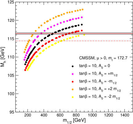
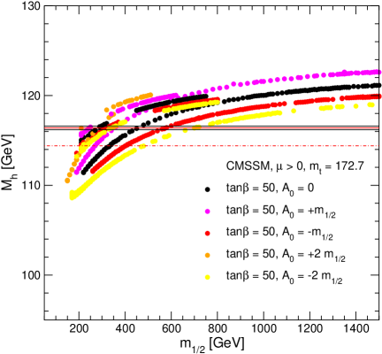
Figure 1: The CMSSM predictions for $M_{h}$ as functions of $m_{1/2}$ with (a) $\tan\beta=10$ and (b) $\tan\beta=50$ for various $A_{0}$. A hypothetical LHC measurement is shown, namely $M_{h}=116.4\pm 0.2\,\,\mathrm{GeV}$, as well as the present 95% C.L. exclusion limit of $114.4\,\,\mathrm{GeV}$.

In our previous analysis, we simply applied a cut-off on $M_{h}$, considering only parameter choices for which FeynHiggs gave $M_{h}>113.0\,\,\mathrm{GeV}$. However, now that the $M_{h}$ constraint assumes greater importance, here we use more completely the likelihood information available from LEP. Accordingly, we evaluate as follows the $M_{h}$ contribution to the overall $\chi^{2}$ function . Our starting points are the $CL_{s}(M_{h})$ values provided by the final LEP results on the SM Higgs boson search, see Fig. 9 in [19] . We obtain by inversion from $CL_{s}(M_{h})$ the corresponding value of ${\tilde{\chi}}^{2}(M_{h})$ determined from [90]

$$\frac{1}{2}{\rm erfc}(\sqrt{\frac{1}{2}\tilde{\chi}^{2}(M_{h})})\equiv CL_{s}(M_{h})~{},$$ (18)

and note the fact that $CL_{s}(M_{h}=116.4\,\,\mathrm{GeV})=0.5$ implies that $\tilde{\chi}^{2}(116.4\,\,\mathrm{GeV})=0$ as is appropriate for a one-sided limit. Correspondingly we set $\tilde{\chi}^{2}(M_{h}>116.4\,\,\mathrm{GeV})=0$. The theory uncertainty is included by convolving the likelihood function associated with $\tilde{\chi}^{2}(M_{h})$ and a Gaussian function, $\tilde{\Phi}(x)$, normalized to unity and centred around $M_{h}$, whose width is $1.5\,\,\mathrm{GeV}$:

$$\chi^{2}(M_{h})=-2\log\left(\int_{-\infty}^{\infty}e^{-\tilde{\chi}^{2}(x)/2}\;\tilde{\Phi}(M_{h}-x)\,{\rm d}x\right)~{}.$$ (19)

In this way, a theoretical uncertainty of up to $3\,\,\mathrm{GeV}$ is assigned for $\sim 95\%$ of all $M_{h}$ values corresponding to one parameter point. The final $\chi^{2}_{M_{h}}$ is then obtained as

$$\chi^{2}_{M_{h}}=\chi^{2}(M_{h})-\chi^{2}(116.4\,\,\mathrm{GeV}) {\rm~{}for~{}} M_{h}\leq 116.4\,\,\mathrm{GeV}~{},$$ (20)

$$\chi^{2}_{M_{h}}=0 {\rm~{}for~{}} M_{h}>116.4\,\,\mathrm{GeV}~{},$$ (21)

and is then combined with the corresponding quantities for the other observables we consider, see eq. (1).

3 Updated CMSSM analysis

As already mentioned, in our previous analysis of the CMSSM [1] we used the range $m_{t}=178.0\pm 4.3\,\,\mathrm{GeV}$ that was then preferred by direct measurements [17]. The preferred range evolved subsequently to $172.7\pm 2.9\,\,\mathrm{GeV}$ [18]. In view of this past evolution and possible future developments, in this Section we first analyze the current situation in some detail, emphasizing some new aspects related to the lower value of $m_{t}$, and then provide a guide to possible future developments.

The effects of the lower $m_{t}$ value are threefold. First, it drives the SM prediction of $M_{W}$ and $\sin^{2}\theta_{\mathrm{eff}}$ slightly further away from the current experimental value (whereas $(g-2)_{\mu}$ and ${\rm BR}(b\to s\gamma)$ are little affected). This increases the favoured magnitude of the supersymmetric contributions, i.e., it effectively lowers the preferred supersymmetric mass scale. Secondly, the predicted value of the lightest Higgs boson mass in the MSSM is lowered by the new $m_{t}$ value, see, e.g., Ref. [91] and Fig. 1. The effects on the electroweak precision observables of the downward shift in $M_{h}$ are minimal, but the LEP Higgs bounds [19, 20] now impose a more important constraint on the MSSM parameter space, notably on $m_{1/2}$. In our previous analysis, we rejected all parameter points for which FeynHiggs yielded $M_{h}<113\,\,\mathrm{GeV}$. The best fit values in Ref. [1] corresponded to relatively small values of $M_{h}$, a feature that is even more pronounced for the new $m_{t}$ value. Thirdly, the focus-point region of the CMSSM parameter space now appears at considerably lower $m_{0}$ than previously, increasing its importance for the $\chi^{2}$ analysis.

In view of all these effects, we now update our previous analysis of the phenomenological constraints on the supersymmetric mass scale $m_{1/2}$ in the CMSSM using the new, lower value  of $m_{t}$ and including a $\chi^{2}$ contribution from $M_{h}$, evaluated as discussed in the previous Section. As in Ref. [1] we use the experimental information on the cold dark matter density from WMAP and other observations to reduce the dimensionality of the CMSSM parameter space. In the parameter region considered in our analysis we find an acceptable dark matter relic density along coannihilation strips, in the Higgs funnel region and in the focus-point region. We comment below on the behaviours of the $\chi^{2}$ function in each of these regions.

As seen in the first panel of Fig. 2, which displays the behaviour of the $\chi^{2}$ function out to the tips of typical WMAP coannihilation strips, the qualitative feature observed in Ref. [1] of a pronounced minimum in $\chi^{2}$ at $m_{1/2}$ for $\tan\beta=10$ is also present for the new value of $m_{t}$. However, the $\chi^{2}$ curve now depends more strongly on the value of $A_{0}$, corresponding to its strong impact on $M_{h}$, as seen in Fig. 1. Values of $A_{0}/m_{1/2}<-1$ are disfavoured at the 90% C.L., essentially because of their lower $M_{h}$ values, but $A_{0}/m_{1/2}=2$ and 1 give equally good fits and descriptions of the data. The old best fit point in Ref. [1] had $A_{0}/m_{1/2}=-1$, but there all $A_{0}/m_{1/2}$ gave a similarly good description of the experimental data. The minimum $\chi^{2}$ value is slightly below 3. This is somewhat higher than the result in Ref. [1], but still represents a good overall fit to the experimental data. The rise in the minimum value of $\chi^{2}$, compared to Ref. [1], is essentially a consequence of the lower experimental central value of $m_{t}$, and the consequent greater impact of the LEP constraint on $M_{h}$ [19, 20]. In the cases of the observables $M_{W}$ and $\sin^{2}\theta_{\mathrm{eff}}$, a smaller value of $m_{t}$ induces a preference for a smaller value of $m_{1/2}$, but the opposite is true for the Higgs mass bound. The rise in the minimum value of $\chi^{2}$ reflects the correspondingly increased tension between the electroweak precision observables and the $M_{h}$ constraint.

A breakdown of the contributions to $\chi^{2}$ from the different observables can be found for some example points in Table 1. The best-fit points for $\tan\beta=10$ and 50 are shown in the first and third lines, respectively. The second line shows a point near the tip of the WMAP coannihilation strip for $\tan\beta=10$, the fourth line shows a point at the tip of the rapid-annihilation Higgs funnel for $\tan\beta=50$. The fifth till the seventh row show points in the focus point region (see below) for $\tan\beta=50$ with low, intermediate and high $m_{1/2}$. It is instructive to compare the contributions to $\chi^{2}$ at the best-fit points with those at the coannihilation, Higgs funnel and focus points. One can see that, for large $m_{1/2}$ values in all the different regions, $(g-2)_{\mu}$ always gives the dominant contribution. However, with the new lower experimental value of $m_{t}$ also $M_{W}$ and $\sin^{2}\theta_{\mathrm{eff}}$ give substantial contributions, adding up to more than 50% of the $(g-2)_{\mu}$ contribution at the coannihilation and Higgs funnel points. On the other hand, $M_{h}$ and ${\rm BR}(b\to s\gamma)$ make negligible contributions to $\chi^{2}$ at these points. As seen from the last lines of the Table, the situation may be different in the focus-point region for low $m_{1/2}$: the first example given yields a reasonably good description of $M_{W}$, $\sin^{2}\theta_{\mathrm{eff}}$ and even $(g-2)_{\mu}$, while the largest contribution to $\chi^{2}$ arises from ${\rm BR}(b\to s\gamma)$ . This smoothly changes to the behavior for large $m_{1/2}$ as described above also in the focus-point region, as can be seen from the last two rows in Tab. 1.

$\tan\beta$	$m_{1/2}$	$m_{0}$	$A_{0}$	comment	$\chi^{2}_{\rm tot}$	$M_{W}$	$\sin^{2}\theta_{\mathrm{eff}}$	$(g-2)_{\mu}$	$b\to s\gamma$	$M_{h}$
10	320	90	320	best fit	2.55	1.01	0.12	0.63	0.23	0.52
10	880	270	1760	bad fit	9.71	2.29	1.28	6.14	0.01	0
50	570	390	-570	best fit	2.79	1.44	0.31	0.08	0.91	0.04
50	1910	1500	-1910	bad fit	9.61	2.21	1.11	6.29	0.01	0
50	250	1320	-250	focus	7.34	0.89	0.15	1.69	3.76	0.84
50	330	1640	-330	focus	6.06	1.24	0.28	3.21	1.33	0
50	800	2970	-800	focus	8.73	1.92	0.72	6.05	0.04	0

Table 1: Breakdown of $\chi^{2}$ contributions from the different precision observables to $\chi^{2}_{\rm tot}$ for some example points. All masses are in GeV. The first and third rows are the best fits for $\tan\beta=10$ and 50, the second row is representative of the coannihilation strip, the fourth row is representative of the Higgs funnel region, and the last three rows are representatives of the focus point-region.

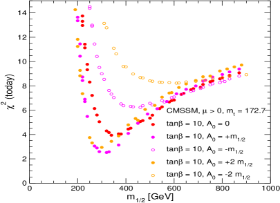
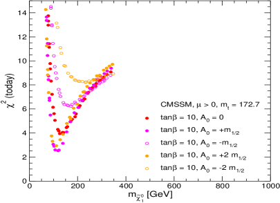
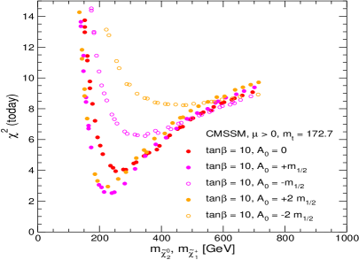
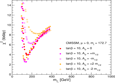
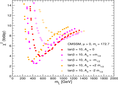
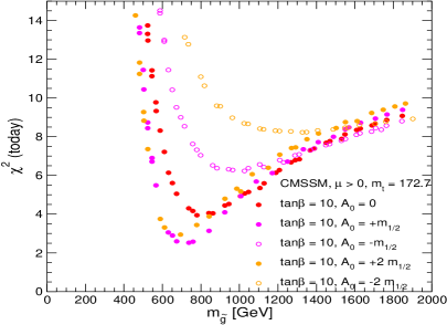
\begin{picture}(0.0,0.0) \put(0.0,0.0){} \put(0.0,0.0){} \put(0.0,0.0){} \put(0.0,0.0){} \put(0.0,0.0){} \put(0.0,0.0){} \put(0.0,0.0){} \put(0.0,0.0){} \put(0.0,0.0){} \put(0.0,0.0){} \put(0.0,0.0){} \put(0.0,0.0){} \put(0.0,0.0){} \put(0.0,0.0){} \end{picture}

Figure 2: The combined likelihood function $\chi^{2}$ for the electroweak observables $M_{W}$, $\sin^{2}\theta_{\mathrm{eff}}$, $(g-2)_{\mu}$, ${\rm BR}(b\to s\gamma)$, and $M_{h}$ evaluated in the CMSSM for $\tan\beta=10$, $m_{t}=172.7\pm 2.9\,\,\mathrm{GeV}$ and various discrete values of $A_{0}$, with $m_{0}$ then chosen to yield the central value of the relic neutralino density indicated by WMAP and other observations. We display the $\chi^{2}$ function for (a) $m_{1/2}$, (b) $m_{\tilde{\chi}^{0}_{1}}$, (c) $m_{\tilde{\chi}^{0}_{2}},m_{\tilde{\chi}^{\pm}_{1}}$, (d) $m_{\tilde{\tau}_{1}}$, (e) $m_{\tilde{t}_{1}}$ and (f) $m_{\tilde{g}}$.

The remaining panels of Fig. 2 update our previous analyses [1] of the $\chi^{2}$ functions for various sparticle masses within the CMSSM, namely the lightest neutralino $\tilde{\chi}^{0}_{1}$, the second-lightest neutralino $\tilde{\chi}^{0}_{2}$ and the (almost degenerate) lighter chargino $\tilde{\chi}^{\pm}_{1}$, the lightest slepton which is the lighter stau $\tilde{\tau}_{1}$, the lighter stop squark $\tilde{t}_{1}$, and the gluino $\tilde{g}$. Reflecting the behaviour of the global $\chi^{2}$ function in the first panel of Fig. 2, the changes in the optimal values of the sparticle masses are not large. The 90% C.L. upper bounds on the particle masses are nearly unchanged compared to the results for $m_{t}=178.0\pm 4.3\,\,\mathrm{GeV}$ given in Ref. [1].

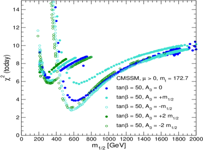
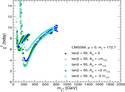
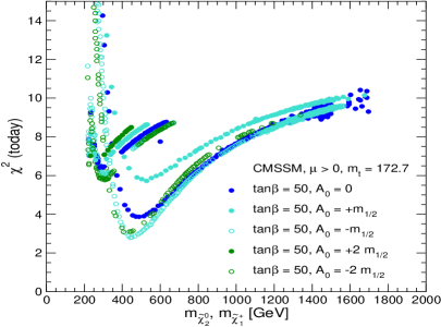
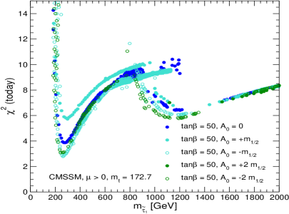
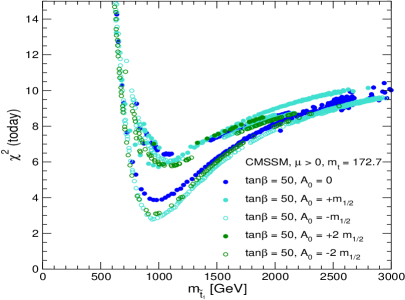
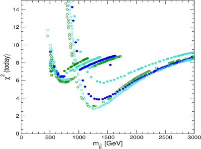
\begin{picture}(0.0,0.0) \put(0.0,0.0){} \put(0.0,0.0){} \put(0.0,0.0){} \put(0.0,0.0){} \put(0.0,0.0){} \put(0.0,0.0){} \put(0.0,0.0){} \put(0.0,0.0){} \put(0.0,0.0){} \put(0.0,0.0){} \put(0.0,0.0){} \put(0.0,0.0){} \put(0.0,0.0){} \put(0.0,0.0){} \end{picture}

Figure 3: As in Fig. 2, but now for $\tan\beta=50$.

The corresponding results for WMAP strips in the coannihilation, Higgs funnel and focus-point regions for the case $\tan\beta=50$ are shown in Fig. 3. The spread of points with identical values of $A_{0}$ at large $m_{1/2}$ is due to the broadening and bifurcation of the WMAP strip in the Higgs funnel region, and the higher set of $\chi^{2}$ curves originate in the focus-point region, as discussed in more detail below. We see in panel (a) that the minimum value of $\chi^{2}$ for the fit with $m_{t}=172.7\pm 2.9\,\,\mathrm{GeV}$ is larger by about a unit than in our previous analysis with $m_{t}=178.0\pm 4.3\,\,\mathrm{GeV}$. Because of the rise in $\chi^{2}$ for the $\tan\beta=10$ case, however, the minimum values of $\chi^{2}$ are now very similar for the two values of $\tan\beta$ shown here. The dip in the $\chi^{2}$ function for $\tan\beta=50$ is somewhat steeper than in the previous analysis, since the high values of $m_{1/2}$ are slightly more disfavoured due to their $M_{W}$ and $\sin^{2}\theta_{\mathrm{eff}}$ values. The best fit values of $m_{1/2}$ are very similar to their previous values. The preferred values of the sparticle masses are shown in the remaining panels of Fig. 3. Due to the somewhat steeper $\chi^{2}$ behavior, the preferred ranges have slightly lower masses than in Ref. [1].

We now return to one novel feature as compared to Ref. [1], namely the appearance of a group of points with moderately high $\chi^{2}$ that have relatively small $m_{1/2}\sim 200\,\,\mathrm{GeV}$. These points have relatively large values of $m_{0}$, as reflected in the relatively large values of $m_{\tilde{\tau}_{1}}$ and $m_{\tilde{t}_{1}}$ seen in panels (d) and (e) of Fig. 3. These points are located in the focus-point region of the $(m_{1/2},m_{0})$ plane [92], where the LSP has a larger Higgsino content, whose enhanced annihilation rate brings the relic density down into the range allowed by WMAP. By comparison with our previous analysis, the focus-point region appears at considerably lower values of $m_{0}$, because of the reduction in the central value of $m_{t}$. This focus-point strip extends to larger values of $m_{0}$ and hence $m_{1/2}$ that are not shown. The least-disfavoured focus points have a $\Delta\chi^{2}$ of at least 3.3 (see the discussion of Table 1 above), and most of them are excluded at the 90% C.L.

Taken at face value, the preferred ranges for the sparticle masses shown in Figs. 2 and 3 are quite encouraging for both the LHC and the ILC. The gluino and squarks lie comfortably within the early LHC discovery range, and several electroweakly-interacting sparticles would be accessible to ILC(500) (the ILC running at $\sqrt{s}=500\,\,\mathrm{GeV}$). The best-fit CMSSM point is quite similar to the benchmark point SPS1a [93] (which is close to point B of Ref. [94]) which has been shown to offer good experimental prospects for both the LHC and ILC [95]. The prospects for sparticle detection are also quite good in the least-disfavoured part of the focus-point region for $\tan\beta=50$ shown in Figs. 3, with the exception of the relatively heavy squarks.

As indicated in Tab. 1 above, the minimum values of $\chi^{2}$ are 2.5 for $\tan\beta=10$ and 2.8 for $\tan\beta=50$, found for $m_{1/2}\sim 320,570\,\,\mathrm{GeV}$ and $A_{0}=+m_{1/2},-m_{1/2}$, respectively, revealing no preference for either large or small $\tan\beta$  . We display in Fig. 4 the $\chi^{2}$ functions for two intermediate values of $\tan\beta=20,35$, for the cases $A_{0}=0,\pm m_{1/2}$. The minima of $\chi^{2}$ are 2.2 and 2.5, respectively, which are not significantly different from the values when $\tan\beta=10,50$. Thus, this analysis reveals no preference for intermediate values of $\tan\beta$, either. The $\chi^{2}$ minima are found for $A_{0}=0,-m_{1/2}$, respectively. They appear when $m_{1/2}\sim 400,500\,\,\mathrm{GeV}$, values intermediate between the locations of the minima for $\tan\beta=10,50$, demonstrating the general stability of this analysis.

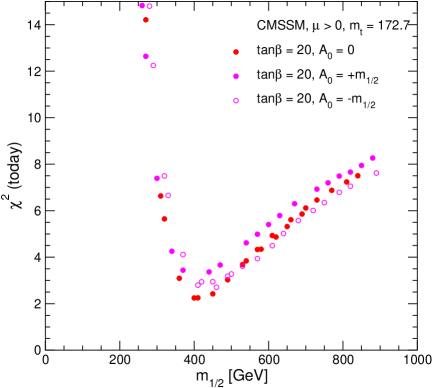
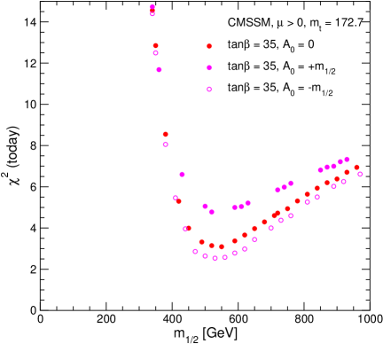
Figure 4: The $\chi^{2}$ functions for $\tan\beta=20,35$ and $A_{0}=0,\pm m_{1/2}$.

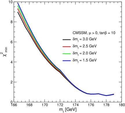
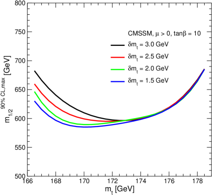
\begin{picture}(0.0,0.0) \put(0.0,0.0){} \put(0.0,0.0){} \end{picture}

Figure 5: The dependence of (a) the minimum value of the $\chi^{2}$ distribution, $\chi^{2}_{\rm min}$, and (b) the 90% C.L. upper limit for $m_{1/2}$ on $m_{t}$ and its experimental error $\delta m_{t}$, keeping the experimental values and theoretical predictions for the other precision observables unchanged.

$m_{t}$	$m_{1/2}$	$m_{0}$	$A_{0}$	$M_{h}$	$\chi^{2}_{\rm tot}$	$M_{W}$	$\sin^{2}\theta_{\mathrm{eff}}$	$(g-2)_{\mu}$	$b\to s\gamma$	$M_{h}$
168	270	80	270	111.5	10.10	1.79	0.14	0.01	0.60	7.57
168	370	100	370	113.5	8.81	3.43	1.02	1.56	0.06	2.73
168	530	140	530	115.3	10.32	4.11	1.63	3.98	0.00	0.60
168	800	210	800	116.9	13.09	4.87	2.45	5.77	0.00	0.00
168	200	80	400	111.1	17.69	0.57	0.06	1.86	6.72	8.49
168	300	100	600	114.1	7.11	2.90	0.68	0.50	1.19	1.83
168	520	160	1040	117.2	10.07	4.20	1.71	4.08	0.08	0.00
168	820	250	1640	118.8	13.70	5.08	2.66	5.95	0.01	0.00
173	190	70	190	111.1	17.20	0.03	0.36	4.56	3.78	8.49
173	270	80	270	114.2	2.72	0.29	0.05	0.01	0.68	1.70
173	330	90	330	115.8	2.24	0.91	0.08	0.80	0.19	0.27
173	370	100	370	116.6	2.95	1.12	0.18	1.56	0.08	0.00
173	530	140	530	118.8	6.02	1.54	0.49	3.98	0.00	0.00
173	800	210	800	120.7	8.80	2.04	0.99	5.77	0.00	0.00
173	170	80	340	112.1	25.10	0.02	0.40	6.21	12.57	5.91
173	200	80	400	113.7	12.12	0.00	0.70	1.85	7.15	2.41
173	300	100	600	117.2	2.70	0.82	0.06	0.50	1.31	0.00
173	520	160	1040	120.8	6.32	1.61	0.54	4.08	0.09	0.00
173	820	250	1640	122.9	9.27	2.18	1.13	5.95	0.01	0.00
178	210	60	0	112.5	10.68	0.34	1.43	3.25	0.70	4.93
178	240	60	0	113.8	5.38	0.41	1.52	0.76	0.27	2.41
178	330	80	0	116.7	0.76	0.01	0.17	0.58	0.00	0.00
178	450	110	0	119.0	2.89	0.11	0.00	2.76	0.02	0.00
178	600	140	0	120.9	4.75	0.22	0.02	4.48	0.03	0.00
178	800	190	0	122.4	6.19	0.36	0.13	5.67	0.02	0.00
178	190	70	190	113.6	13.26	0.43	1.51	4.56	4.03	2.73
178	270	80	270	117.1	1.53	0.08	0.68	0.01	0.77	0.00
178	330	90	330	119.0	1.14	0.02	0.10	0.80	0.23	0.00
178	370	100	370	119.9	1.76	0.06	0.03	1.56	0.10	0.00
178	530	140	530	122.4	4.20	0.20	0.01	3.98	0.00	0.00
178	800	210	800	124.7	6.35	0.41	0.17	5.77	0.00	0.00

Table 2: Breakdown of $\chi^{2}$ contributions from the different precision observables to $\chi^{2}_{\rm tot}$ for some example points with $m_{t}=168,173,178\,\,\mathrm{GeV}$, $\delta m_{t}=2.5\,\,\mathrm{GeV}$ and $\tan\beta=10$. All masses shown are in GeV. The fifth column shows the $M_{h}$ value for the corresponding point, and the last column shows the $\chi^{2}$ contribution of this $M_{h}$ value. The values of $A_{0}$ were selected so as to minimize $\chi^{2}_{\rm tot}$ for the corresponding value of $m_{1/2}$.

In view of the possible future evolution of both the central value of $m_{t}$ and its experimental uncertainty $\delta m_{t}$, we have analyzed the behaviour of the global $\chi^{2}$ function for $166\,\,\mathrm{GeV}<m_{t}<179\,\,\mathrm{GeV}$ and $1.5\,\,\mathrm{GeV}<\delta m_{t}<3.0\,\,\mathrm{GeV}$ for the case of $\tan\beta=10$ (assuming that the experimental results and theoretical predictions for the precision observables are otherwise unchanged), as seen in the left panel of Fig. 5. We see that the minimum value of $\chi^{2}$ is almost independent of the uncertainty $\delta m_{t}$, but increases noticeably as the assumed central value of $m_{t}$ decreases. This effect is not strong when $m_{t}$ decreases from $178.0\,\,\mathrm{GeV}$ to $172.7\,\,\mathrm{GeV}$, but does become significant for $m_{t}<170\,\,\mathrm{GeV}$. This effect is not independent of the known preference of the ensemble of precision electroweak data for $m_{t}\sim 175\,\,\mathrm{GeV}$ within the SM [39, 40], to which the observables $M_{W}$ and $\sin^{2}\theta_{\mathrm{eff}}$ used here make important contributions. On the other hand, as already commented, within the CMSSM there is the additional effect that the best fit values of $m_{1/2}$ for very low $m_{t}$ result in $M_{h}$ values that are excluded by the LEP Higgs searches [19, 20] and have a very large $\chi^{2}_{M_{h}}$, resulting in an increase of the lowest possible $\chi^{2}$ value for a given top-quark mass value. This effect also increases the value of $m_{1/2}$ where the $\chi^{2}$ function is minimized. This is analyzed in more detail in Table 2, where we show the breakdown of the different contributions to $\chi^{2}$ for $m_{t}=168,173,178\,\,\mathrm{GeV}$ for $\delta m_{t}=2.5\,\,\mathrm{GeV}$ and $\tan\beta=10$. The $A_{0}$ values are chosen so as to minimize $\chi^{2}_{\rm tot}$ for each choice of $m_{1/2}$. For $m_{t}=168\,\,\mathrm{GeV}$, $\chi^{2}_{\rm tot}$ exhibits only a shallow and relatively high minimum, and $M_{h}$ and ${\rm BR}(b\to s\gamma)$ give the largest contribution for low $m_{1/2}$, shifting smoothly to large contributions from $M_{W}$, $\sin^{2}\theta_{\mathrm{eff}}$ and $(g-2)_{\mu}$ for larger $m_{1/2}$. For $m_{t}=173\,\,\mathrm{GeV}$, a more pronounced minimum of $\chi^{2}_{\rm tot}$ appears for relatively small $m_{1/2}$ values. For lower $m_{1/2}$, again $M_{h}$ and ${\rm BR}(b\to s\gamma)$ give large contributions, whereas for higher values this shifts again to $M_{W}$, $\sin^{2}\theta_{\mathrm{eff}}$ and $(g-2)_{\mu}$, after passing through a minimum with a very good fit quality where no single contribution exceeds unity. The same trend, just slightly more pronounced, can be observed for $m_{t}=178\,\,\mathrm{GeV}$. Finally, in the right panel of Fig. 5 we demonstrate that the 90% C.L. upper limit on $m_{1/2}$ shows only a small variation, less than 10% for $m_{t}$ in the preferred range above $170\,\,\mathrm{GeV}$ . Finally we note that the upper limit on $m_{1/2}$ is essentially independent of $\delta m_{t}$ .

It is striking that the preference noted earlier for relatively low values of $m_{1/2}$ remains almost unaltered after the change in $m_{t}$ and the change in the treatment of the LEP lower limit on $M_{h}$. There seems to be little chance at present of evading the preference for small $m_{1/2}$ hinted by the present measurements of $M_{W}$, $\sin^{2}\theta_{\mathrm{eff}}$, ${\rm BR}(b\to s\gamma)$ and $(g-2)_{\mu}$, at least within the CMSSM framework. It should be noted that the preference for a relatively low SUSY scale is correlated with the top mass value lying in the interval $170\,\,\mathrm{GeV}\;\raisebox{-3.00003pt}{$\stackrel{{\scriptstyle\displaystyle<}}{{\sim}}$}\;m_{t}\;\raisebox{-3.00003pt}{$\stackrel{{\scriptstyle\displaystyle<}}{{\sim}}$}\;180\,\,\mathrm{GeV}$.

4 NUHM Analysis

In the NUHM, one may parametrize the soft supersymmetry-breaking contributions to the squared masses of the two Higgs multiplets, $m_{1,2}^{2}$, as follows:

$$m_{i}^{2}\;=\;m_{0}^{2}(1+\delta_{i})~{},$$ (22)

where $m_{0}^{2}$ is the (supposedly) universal soft supersymmetry-breaking squared mass for the squarks and sleptons. As already mentioned, the increase of the dimensionality of the NUHM parameter space compared to the CMSSM, due to the appearance of the two new parameters $\delta_{1,2}$, makes a systematic survey quite involved. Here, as illustrations of what may happen in the NUHM, we analyze some specific parameter planes that generalize certain specific CMSSM points. We note that certain combinations of input parameter choices lead to soft SUSY-breaking Higgs mass squares which are negative at the GUT scale. When either $m_{1}^{2}+\mu^{2}<0$ or $m_{2}^{2}+\mu^{2}<0$, the point is excluded, so as to ensure vacuum stability at the GUT scale [6].

Since it is the value of $m_{1/2}$ that affects most importantly the masses of the sparticles that might be observable at the LHC or ILC, our primary objective is to investigate whether the introduction of extra NUHM parameters affects significantly the preference for small $m_{1/2}$ found previously within the CMSSM: see Figs. 6 and 7. After satisfying ourselves on this point, we subsequently explore the possible dependences on $M_{A}$ and $\mu$: see Fig. 8. In order to present our results we use parameter planes with generic points that do not necessarily satisfy the CDM constraint. Exhibiting full parameter planes rather than just the regions where the neutralino relic density respects the WMAP limits (we indicate these strips in the plots) provides a better understanding of the dependences of the $\chi^{2}$ function on the different NUHM variables. It also provides a context for understanding the branchings of the $\chi^{2}$ function visible in Fig. 9, which are due to the bifurcations of the WMAP strips in the parameter planes. We also note that, in NUHM models with a light gravitino where the CDM constraint does not apply, generic regions of these parameter planes may be consistent with cosmology.

In view of our primary objective, Fig. 6 shows two examples of $(m_{1/2},m_{0})$ planes for fixed values of $\mu,M_{A},A_{0}$ and $\tan\beta$ (top row) and two examples of $(m_{1/2},\mu)$ planes for fixed values of $m_{0},M_{A},A_{0}$ and $\tan\beta$ (bottom row). In both the two top panels, the left boundaries of the shaded regions are provided by the LEP lower limit on the chargino mass, the upper bounds on $m_{1/2}$ are provided by the GUT stability constraint, and the lower edges of the shaded regions are provided by the stau LSP constraint. The colour codings are as follows. In each panel, the best fit NUHM point that respects the WMAP constraints on the relic neutralino density is marked by a (blue) plus sign, and the (blue) cross indicates the CMSSM values of $(m_{1/2},m_{0})$ [or $(m_{1/2},\mu)$] for the chosen values of the other parameters. The green (medium grey) regions have $\Delta\chi^{2}<1$ relative to the minimum when the WMAP/CDM constraint is not employed. Hence, some points in this region may have a lower $\chi^{2}$ than our best fit point when the CDM constraint is employed.

In all four panels of Fig. 6, our best CDM fit, denoted by the plus sign, is within 1 sigma of the overall minimum $\chi^{2}$, and hence lies within the green region. The yellow (light grey) regions have $\Delta\chi^{2}<3.84$, and the black points have larger values of $\Delta\chi^{2}$ relative to the absolute minimum. Traversing the regions with $\Delta\chi^{2}<1,3.84$, there are thin, darker shaded strips where the relic neutralino density lies within the range favoured by WMAP. That is, in these regions, $\chi^{2}$ is within 1 or 3.84 of the minimum $\chi^{2}$ when the WMAP/CDM bound is included. The blue cross must always lie within these regions. Our sampling procedure causes these WMAP strips to appear intermittent. In the top right panel of Fig. 6, we note two vertical tramlines, which are due to rapid annihilation via the direct-channel $A$ pole. Since $M_{A}$ is fixed in each of these panels, there is always a value of $m_{1/2}$ such that $2m_{\tilde{\chi}^{0}_{1}}\approx M_{A}$, in principle even for $\tan\beta=10$. We note that the analogous tramlines are invisible in panel (a), because they have a $\Delta\chi^{2}>4$ and thus would be located in the black shaded region.

In the lower two panels, large values of $\mu$ are excluded due to the GUT constraint, large values of $m_{1/2}$ are excluded by the stau LSP constraint, and low values of $\mu$ and $m_{1/2}$ are exuded by the chargino mass limit. In the lower left panel, large values of $m_{1/2}$ are excluded because the ${\tilde{\tau}}_{1}$ becomes the LSP, whereas in the right panel our computation was limited to $m_{1/2}<1000\,\,\mathrm{GeV}$, thus producing the right-hand boundary. Within the regions allowed by these constraints, the same colour codings are used. In the lower right panel, one sees clearly the effect of the pseudoscalar funnel at $m_{1/2}\approx 680\,\,\mathrm{GeV}$. In the lower left panel, this possibility is excluded by the GUT stability constraint.

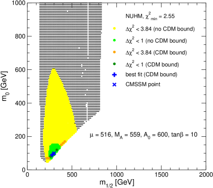
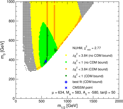
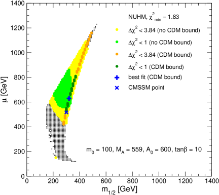
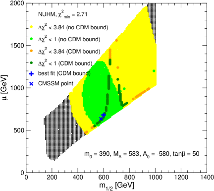
\begin{picture}(0.0,0.0) \put(0.0,0.0){} \put(0.0,0.0){} \put(0.0,0.0){} \put(0.0,0.0){} \put(0.0,0.0){} \put(0.0,0.0){} \end{picture}

Figure 6: Sample NUHM scenarios shown in the ($m_{1/2},m_{0}$) plane (top row) and ($m_{1/2},\mu$) plane (bottom row). The CMSSM points shown in the left (right) column correspond to the best fit points for $\tan\beta=10\;(50)$. The other parameters are given in the plots. The green [medium grey] (yellow [light grey]) regions have $\Delta\chi^{2}<1(3.84)$, whilst the black regions have larger $\Delta\chi^{2}$. The strips where the neutralino relic density respects the WMAP limits have darker shadings. The blue plus sign marks the best-fit NUHM point that respects the relic density bounds, and the CMSSM point is marked with a blue cross.

The planes in Fig. 6 have been defined such that the CMSSM points marked by (blue) crosses in the different panels of Fig. 6 lie at the minima of the CMSSM $\chi^{2}$ functions shown in Figs. 2 and 3. They enable us to study whether the CMSSM preference for relatively small $m_{1/2}$ may be perturbed by generalizing to the larger NUHM parameter space. In each case, we see that the CMSSM point lies close to the best NUHM fit, whose $\chi^{2}$ is lower by just 0.00, 0.02, 0.72 and 0.08, respectively. We also note that the ranges of $m_{1/2}$ favoured at this level are quite close to the CMSSM values. Thus, in these cases, the introduction of two extra parameters in the NUHM does not modify the preference for relatively small values of $m_{1/2}$ observed previously in the CMSSM. In the top left panel for $\tan\beta=10$, we see that the preferred range of $m_{0}$ is also very close to the CMSSM value. On the other hand, we see in the top right panel that rather larger values of $m_{0}$ would be allowed for $\tan\beta=50$ at the $\Delta\chi^{2}<1$ level. This is due to the insensitivity of the annihilation cross section to $m_{0}$ in the funnel due to rapid annihilation via the pseudoscalar Higgs boson $A$. We also see in the bottom two panels that quite wide ranges of $\mu$ would be allowed for either value of $\tan\beta$ .

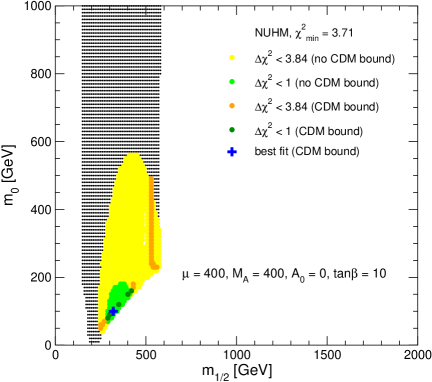
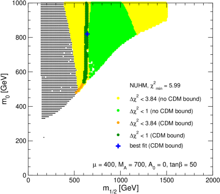
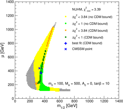
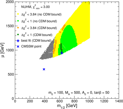
\begin{picture}(0.0,0.0) \put(0.0,0.0){} \put(0.0,0.0){} \put(0.0,0.0){} \put(0.0,0.0){} \put(0.0,0.0){} \put(0.0,0.0){} \end{picture}

Figure 7: Additional sample NUHM scenarios shown in the ($m_{1/2},m_{0}$) plane (top row) and ($m_{1/2},\mu$) plane (bottom row). The colour coding is the same as in Fig. 6.

Fig. 7 displays four analogous NUHM planes, specified this time by values of $\mu,M_{A}$ and $A_{0}$ in the top row and $m_{0},M_{A},A_{0}$ in the bottom row that do not correspond to minima of the $\chi^{2}$ function for the CMSSM with the corresponding values of $\tan\beta$. These examples were studied in detail in [6], and enable us to explore whether there may be good NUHM fits that are not closely related to the best CMSSM fits. In the top panels, the left boundaries are due to the chargino constraint, and the bottom boundaries are due to the stau LSP constraint. In the left panel, the right boundary is due to GUT stability, but in the right panel it is due to a sampling limit. In the bottom left panel the GUT, stau and chargino constraints operate similarly as in Fig. 6, and the tail at low $\mu$ and large $m_{1/2}$ is truncated by the GUT stability constraint. In the bottom right panel, the top boundary is due to GUT stability, the bottom boundary to the stau, and the boundary at large $m_{1/2}$ is another sampling limitation . Within the allowed regions of Fig. 7, the colour codings are the same as in Fig. 6. The best fit CDM point lies within the $\Delta\chi^{2}<1$ green regions in the top left and bottom right panels, whereas in the upper right panel the best fit point has $\Delta\chi^{2}$ slightly larger than 1, and its $\Delta\chi^{2}$ is even greater in the bottom left panel.

In the $(m_{1/2},m_{0})$ planes shown in the top row, we see that the ranges of $m_{1/2}$ favoured at the $\Delta\chi^{2}<1$ level are again limited to values close to the best-fit CDM values. The range of $m_{0}$ for a given $\Delta\chi^{2}$ is somewhat restricted for $\tan\beta=10$ (top left), but is again considerably larger for $\tan\beta=50$ (top right). As for the $(m_{1/2},\mu)$ planes in the bottom row, we see in the left panel for $\tan\beta=10$ that the range of $m_{1/2}$ is again restricted at the $\Delta\chi^{2}<1$ level, whereas the range of $\mu$ is almost completely unrestricted. A similar conclusion holds in the bottom right panel for $\tan\beta=50$, though here the range of $m_{1/2}$ is somewhat broader .

Having established that the CMSSM preference for small values of $m_{1/2}$ is generally preserved in the NUHM, whereas different values of $m_{0}$ and $\mu$ are not necessarily disfavoured, we now study further the sensitivity to $\mu$ and $M_{A}$ via the four examples of $(\mu,M_{A})$ planes shown in Fig. 8. In each case, we have made specific choices of $A_{0}$, $\tan\beta$, $m_{1/2}$ and $m_{0}$. In the two panels on the left, these correspond to the best CMSSM fit along the corresponding WMAP strip. The examples on the right were studied in [6]. In each case, we restrict our attention to the regions of the plane that have no vacuum instability below the GUT scale. This constraint provides the near-vertical right-hand edges of the coloured regions, whereas the other boundaries are due to various phenomenological constraints. The near-vertical boundaries at small $\mu$ in the top panels are due to the LEP chargino exclusion, and those in the bottom panels are due to the stau LSP constraint. The boundary at low $M_{A}$ in the top left panel is also due to the stau LSP constraint, whereas that in the top right panel is again the GUT stability constraint.

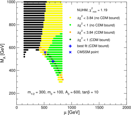
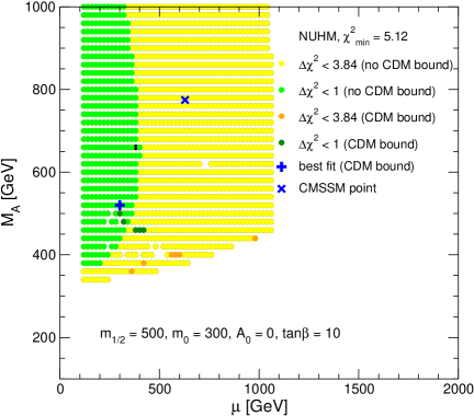
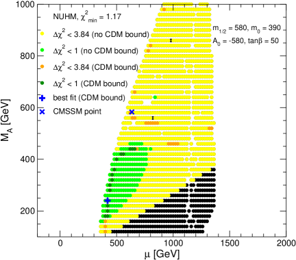
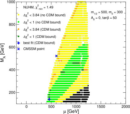
\begin{picture}(0.0,0.0) \put(0.0,0.0){} \put(0.0,0.0){} \put(0.0,0.0){} \put(0.0,0.0){} \put(0.0,0.0){} \put(0.0,0.0){} \put(0.0,0.0){} \put(0.0,0.0){} \put(0.0,0.0){} \put(0.0,0.0){} \put(0.0,0.0){} \put(0.0,0.0){} \put(0.0,0.0){} \put(0.0,0.0){} \put(0.0,0.0){} \put(0.0,0.0){} \end{picture}

Figure 8: Sample NUHM $(\mu,M_{A})$ planes for different choices of $(m_{1/2},m_{0},A_{0},\tan\beta)$: (a) $(300\,\,\mathrm{GeV},100\,\,\mathrm{GeV},600\,\,\mathrm{GeV},10)$, (b) $(500\,\,\mathrm{GeV},300\,\,\mathrm{GeV},0,10)$, (c) $(580\,\,\mathrm{GeV},390\,\,\mathrm{GeV}$, $-580\,\,\mathrm{GeV},50)$, and (d) $(500\,\,\mathrm{GeV},300\,\,\mathrm{GeV},0,50)$. The colour coding is as in Fig. 6.

Within the allowed regions of Fig. 8, the colour codings are the same as in Fig. 6. We see that in the top left panel the WMAP strip runs parallel to the lower boundary defined by the stau LSP constraint. The best fit NUHM point has $\chi^{2}=1.19$, which is somewhat less than two units smaller than for the CMSSM point. This is hardly significant, and suggests that the absolute minimum of the NUHM $\chi^{2}$ lies at a similar value of $m_{1/2}$. As seen from the location and shape of the green region with $\Delta\chi^{2}<1$, the fit is relatively insensitive to the magnitudes of $\mu$ and $M_{A}$, as long as they are roughly proportional, but small values of $\mu/M_{A}$ are disfavoured. In contrast, for the larger value of $m_{1/2}$ shown in the top right panel of Fig. 8, we see that low values of $\mu$ are preferred. However, the minimum value of $\chi^{2}=5.12$ in the NUHM is not much lower than in the CMSSM, even though it occurs for significantly smaller values of both $\mu$ and $M_{A}$ .

Turning now to the bottom left panel of Fig. 8 for $\tan\beta=50$ and $A_{0}=580\,\,\mathrm{GeV}$, with $m_{1/2}$ and $m_{0}$ again chosen so as to minimize $\chi^{2}$ (i.e., to reproduce the corresponding best-fit point), we note several features familiar from the two previous panels. The WMAP strip clings close to the left boundary of the allowed region, apart from an intermittent funnel straddling the $M_{A}=2m_{\tilde{\chi}^{0}_{1}}$ line. The minimum of $\chi^{2}=1.13$ for the NUHM is somewhat smaller than for the CMSSM. The $\Delta\chi^{2}<1$ NUHM region is a lobe extending away from the origin at small $\mu$ and $M_{A}$. Similar features are seen in the bottom right panel for $\tan\beta=50$ and $A_{0}=0$, except that the $\Delta\chi^{2}<1$ lobe extends up to rather larger values of $\mu$ and $M_{A}$ .

These examples show that, although the absolute values of $\mu$ and $M_{A}$ are typically relatively unconstrained in the NUHM , their values tend to be correlated, often with a restricted range for their ratio: $M_{A}/\mu\sim 1.4,\leq 1,\sim 2$ at the $\Delta\chi^{2}<1$ level in the first three panels of Fig. 8. On the other hand, the correlation in the fourth panel takes the form $M_{A}\sim\frac{1}{2}(\mu-400\,\,\mathrm{GeV}$).

To conclude this Section, we make some remarks about the preferred masses of sparticles and their possible detectability within the NUHM framework, in the light of the above $\chi^{2}$ analysis. Since the ranges of $m_{1/2}$ favoured within the CMSSM are also favoured in the NUHM, one should expect that the LHC prospects for detecting the gluino and several other sparticles may also be quite good in the NUHM. On the other hand, the greater uncertainties in $m_{0},\mu$ and $M_{A}$ suggest that the prospects for sparticle studies at the ILC may be more variable within the NUHM. These remarks are borne out by Figs. 9 and 10, which display $\chi^{2}$ functions for various sparticle masses in a selection of NUHM scenarios. Fig. 9 presents masses in the four NUHM scenarios shown in Fig. 6, in which the CMSSM points correspond to the best-fit points from Sect. 3, and Fig. 10 presents masses in two of the scenarios shown in Fig. 8.

In each panel of Fig. 9, we display the $\chi^{2}$ functions for the masses of the $\tilde{\chi}^{0}_{1}$, $\tilde{\chi}^{0}_{2}/\tilde{\chi}^{\pm}_{1}$, $\tilde{\tau}_{1}$, $\tilde{t}_{1}$ and $\tilde{g}$, for NUHM parameters along the WMAP strips in the corresponding panels of Fig. 6. Since there are several branches of the WMAP strips in some cases, the $\chi^{2}$ functions are sometimes multivalued. In the top left panel of Fig. 9, we see well-defined preferred values for the sparticle masses, with the gluino and stop masses falling comfortably within reach of the LHC, and the $\tilde{\chi}^{0}_{1},\tilde{\tau}_{1}$ and possibly also the $\tilde{\chi}^{0}_{2}$ and $\tilde{\chi}^{\pm}_{1}$ within reach of the ILC(500). When $\Delta\chi^{2}\sim 4.5$, new branches of the $\chi^{2}$ function appear, corresponding to a branching of the WMAP strip around a rapid-annihilation funnel when $M_{A}=559\,\,\mathrm{GeV}\sim 2m_{\tilde{\chi}^{0}_{1}}$. This funnel is not visible in Fig. 6, but would appear in the black-spotted region of large $\Delta\chi^{2}$. The ILC(1000) would have a good chance to see even the lighter stop. Turning to the top right panel of Fig. 9, we see that the branching due to the rapid-annihilation funnel appears at much lower $\Delta\chi^{2}$, reflecting the closeness of the funnel to the best-fit point in the top right panel of Fig. 6. In this case, whereas the ${\tilde{g}}$ should be observable at the LHC, the ${\tilde{t}}_{1}$ might well be problematic . The $\tilde{\chi}^{0}_{1}$ would be kinematically accessible at the ILC(500), but the ${\tilde{\tau}}_{1}$ might well be too heavy: the rises in the branches of its $\chi^{2}$ function at larger masses reflect the extension of the WMAP strip to large $m_{0}$ that is seen in the corresponding panel of Fig. 6. In this particular scenario, the $\tilde{\chi}^{0}_{2}$ and $\tilde{\chi}^{\pm}_{1}$ would probably not be observable at the ILC(500). The ILC(1000) on the other hand, would have a high potential to detect them. The bottom left panel of Fig. 9 has the most canonical $\chi^{2}$ functions: the gluino and stop would very probably lie within reach of the LHC and the $\tilde{\tau}_{1}$ within reach of the ILC(500), whereas the $\tilde{\chi}^{0}_{2}$ and $\tilde{\chi}^{\pm}_{1}$ might be more problematic. Again the ILC(1000) offers much better opportunities here, possibly even for the lighter stop. Finally, the prospective observabilities in the bottom right scenario would be rather similar to those in the top right scenario: we again see that, as one moves away from the coannihilation strip, the $\tilde{\tau}_{1}$ may become much heavier than the $\tilde{\chi}^{0}_{1}$, and too heavy to observe at the ILC(500). The ILC(1000) should, on the other hand, offers very good prospects.

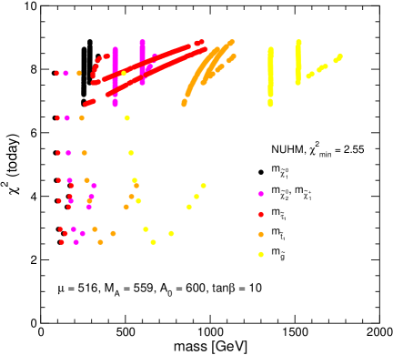
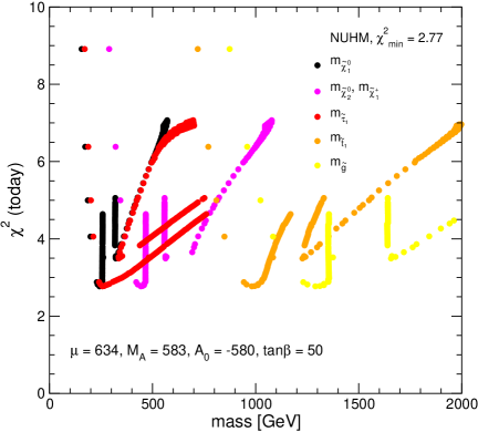
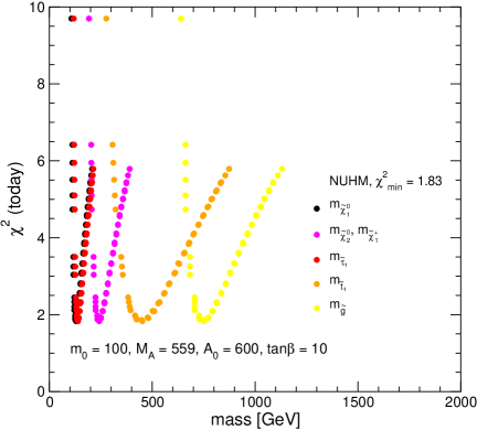
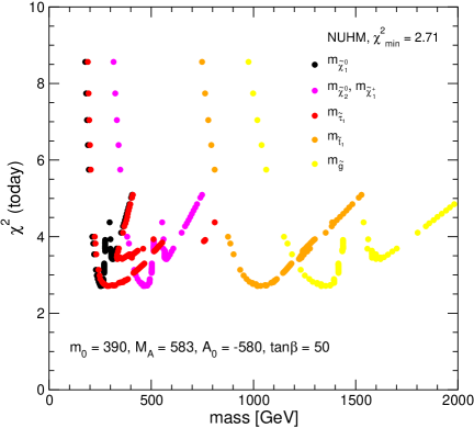
\begin{picture}(0.0,0.0) \put(0.0,0.0){} \put(0.0,0.0){} \put(0.0,0.0){} \put(0.0,0.0){} \put(0.0,0.0){} \put(0.0,0.0){} \end{picture}

Figure 9: The likelihood $\chi^{2}$ along the WMAP strips in the sample NUHM scenarios shown in Fig. 6, as a function of the masses of the $\tilde{\chi}^{0}_{1}$, $\tilde{\chi}^{0}_{2}/\tilde{\chi}^{\pm}_{1}$, $\tilde{\tau}_{1}$, $\tilde{t}_{1}$ and $\tilde{g}$. The branchings in the $\chi^{2}$ curves reflect the corresponding branchings in the WMAP strips in Fig. 6.

Fig. 10 presents a similar analysis of sparticle masses of the two favoured scenarios in Fig. 8, namely in the two left-hand panels. In these cases, we show the variations of the $\chi^{2}$ functions for the different masses as one follows the WMAP strip to larger values of $M_{A}$. In the left panel of Fig. 10, we display the masses of the $\tilde{\chi}^{0}_{2}$ and $\tilde{\chi}^{\pm}_{1}$ (which are nearly equal) in black, the mass of the $\tilde{\chi}^{0}_{3}$ in pink, the masses of the $\tilde{\chi}^{0}_{4}$ and $\tilde{\chi}^{\pm}_{2}$ (which are nearly equal) in red, the mass of the $\tilde{t}_{1}$ in yellow (with black border), and $M_{A}$ in blue. In each case, the $+$ sign of the same colour represents the best fit in the CMSSM for the same values of $m_{1/2},m_{0},A_{0}$ and $\tan\beta$. The fact that the minima of the NUHM lie somewhat below the CMSSM points reflect the fact that the NUHM offers a slightly better fit, but the difference is not significant. In this case, the preferred masses of the $\tilde{\chi}^{0}_{2}$ and $\tilde{\chi}^{\pm}_{1}$ are almost identical to the best-fit CMSSM values, and the same would be true for the $\tilde{\chi}^{0}_{1}$ and $\tilde{g}$, which are not shown. The masses of the $\tilde{\chi}^{0}_{3}$, $\tilde{t}_{1}$ and $A$ are also very similar to their CMSSM values, but the $\tilde{\chi}^{0}_{4}$ and $\tilde{\chi}^{\pm}_{2}$ may be significantly heavier. In addition to the above sparticle masses, the right panel also includes the mass of the $\tilde{\tau}_{1}$ in orange. In this case, whereas the masses of the $\tilde{\chi}^{0}_{1}$ (not shown), $\tilde{\chi}^{0}_{2}/\tilde{\chi}^{\pm}_{1}$ and $\tilde{g}$ (not shown) preferred in the NUHM are similar to their values at the best-fit CMSSM point, this is not true for the other sparticles shown. The $A$ boson may be considerably lighter, the $\tilde{\chi}^{0}_{3}$, $\tilde{\chi}^{0}_{4}$ and the $\tilde{\chi}^{\pm}_{2}$ may be either lighter or heavier, and the $\tilde{\tau}_{1}$ and $\tilde{t}_{1}$ might be significantly heavier for points along the Higgs funnel visible in Fig. 8. Thus, in this case the prospects for detecting some sparticles at the LHC or ILC may differ substantially in the NUHM from the CMSSM.

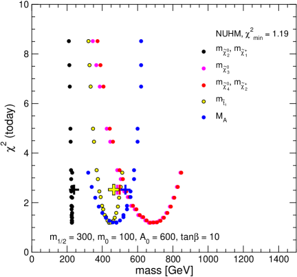
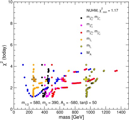
Figure 10: The likelihood $\chi^{2}$ along the WMAP strips in the sample NUHM scenarios shown in the left panels of Fig. 8, as a function of the masses of the $\tilde{\chi}^{0}_{2}/\tilde{\chi}^{\pm}_{1}$ (black), $\tilde{\chi}^{0}_{3}$ (pink), $\tilde{\chi}^{0}_{4}/\tilde{\chi}^{\pm}_{2}$ (red), $\tilde{\tau}_{1}$ (orange) [omitted from the left panel], $\tilde{\tau}_{1}$ (yellow with black border) and $A$ boson (blue). The branchings in the $\chi^{2}$ curves in the right panel reflect the corresponding branchings in the WMAP strips in the bottom left panel of Fig. 8. The crosses indicate the corresponding best fit points in the CMSSM.

To summarize: these examples demonstrate that, although the preferred value of the overall sparticle mass scale set by $m_{1/2}$ may be quite similar in the NUHM to its CMSSM value, the masses of some sparticles in the NUHM may differ significantly from the corresponding CMSSM values.

5 VCMSSM Analysis

As an alternative to the above NUHM generalization of the CMSSM, we now examine particular CMSSM models with the additional constraint $B_{0}=A_{0}-m_{0}$ motivated by minimal supergravity models, namely the VCMSSM framework introduced earlier. We still assume that the gravitino is too heavy to be the LSP. The extra constraint reduces the dimensionality of the VCMSSM parameter space, as compared with the CMSSM, facilitating its exploration. In the CMSSM case, the electroweak vacuum conditions can be used to fix $|\mu|$ and $M_{A}$ as functions of $m_{1/2},m_{0}$ and $A_{0}$ for a large range of fixed values of $\tan\beta$. On the other hand, in the VCMSSM case the expression for $B_{0}$ in terms of $A_{0}$ and $m_{0}$ effectively yields a relation between $|\mu|$ and $M_{A}$ that is satisfied typically for only one value of $\tan\beta$, for any fixed set of $m_{1/2},m_{0}$ and $A_{0}$ values [98, 7].

As already mentioned, motivated by $(g-2)_{\mu}$ and (to a lesser extent) ${\rm BR}(b\to s\gamma)$, we restrict our attention here to the case $\mu>0$. As is well known, other phenomenological constraints tend to favour $\tan\beta\;\raisebox{-3.00003pt}{$\stackrel{{\scriptstyle\displaystyle>}}{{\sim}}$}\;5$, see e.g. Refs. [91, 99]. This condition is generally obeyed along the WMAP coannihilation strip for neutralino dark matter in the VCMSSM if one assumes $A_{0}\geq 0$, in which case the resultant value of $\tan\beta$ tends to increase with $m_{1/2}$ and $m_{0}$ along the WMAP strip. We have studied the choices $A_{0}/m_{0}=0,0.75,3-\sqrt{3}$ and 2. In this Section we restrict our attention to these cases, and in the next Section we compare the VCMSSM results with the corresponding gravitino dark matter scenarios.

Since in the CMSSM the value of $\chi^{2}$ tends first to decrease and then to increase with $m_{1/2}$, but does not vary strongly with $\tan\beta$, we would expect the $\chi^{2}$ function to exhibit a similar dependence on $m_{1/2}$ also in the VCMSSM scenario. This effect is indeed seen in the first panel of Fig. 11: there are well-defined local minima at $m_{1/2}\sim 400$ to 600 GeV, as $A_{0}/m_{0}$ varies from 0 to 2. However, for the latter value of $A_{0}/m_{0}$, we notice some isolated (red) points with $m_{1/2}\sim 140\,\,\mathrm{GeV}$ and much lower $\chi^{2}\sim 2$. At these points, which barely survive the LEP chargino limit, rapid annihilation through a direct-channel light-Higgs pole brings the neutralino relic density down into the WMAP range [24]. The remaining panels of Fig. 11 display the $\chi^{2}$ functions for the masses of the $\tilde{\chi}^{0}_{1},\tilde{\tau}_{1},\tilde{\chi}^{0}_{2},\tilde{\chi}^{\pm}_{1},\tilde{t}_{1}$ and $\tilde{g}$. Their qualitative features are similar to those shown earlier for the CMSSM, with the addition of the exceptional low-mass rapid-annihilation points. In these VCMSSM NDM scenarios, the LHC has good prospects for the $\tilde{g}$ and $\tilde{t}_{1}$ and the ILC(500) has good prospects for the $\tilde{\chi}^{0}_{1}$ and $\tilde{\tau}_{1}$, whereas the prospects for the $\tilde{\chi}^{0}_{2}$ and $\tilde{\chi}^{\pm}_{1}$ would be dimmer, except at the isolated rapid-annihilation points. The ILC(1000), on the other hand, would have a good chance to detect the $\tilde{\chi}^{0}_{2}$ and the $\tilde{\chi}^{\pm}_{1}$, depending somewhat on $A_{0}/m_{0}$. These points might also be accessible to the Tevatron, in particular via searches for gluinos.

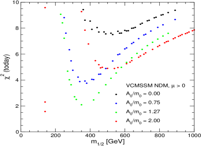
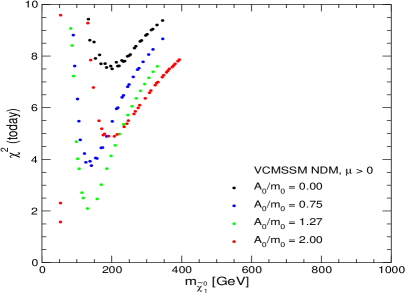
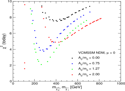
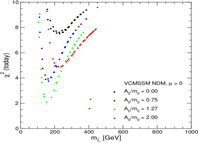
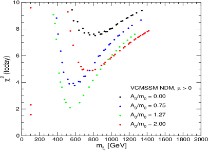
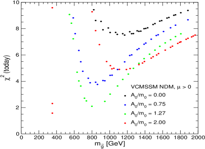
\begin{picture}(0.0,0.0) \put(0.0,0.0){} \put(0.0,0.0){} \put(0.0,0.0){} \put(0.0,0.0){} \put(0.0,0.0){} \put(0.0,0.0){} \put(0.0,0.0){} \put(0.0,0.0){} \put(0.0,0.0){} \put(0.0,0.0){} \end{picture}

Figure 11: The combined likelihood $\chi^{2}$ along the WMAP strips for NDM scenarios with $A_{0}/m_{0}=0,0.75,3-\sqrt{3}$ and $2$, as a function (a) of $m_{1/2}$, (b) of $m_{\tilde{\chi}^{0}_{1}}$, (c) of $m_{\tilde{\chi}^{0}_{2}}$ and $m_{\tilde{\chi}^{\pm}_{1}}$, (d) of $m_{\tilde{\tau}_{1}}$, (e) of $m_{\tilde{t}_{1}}$ and (f) $m_{\tilde{g}}$.

We find no analogous focus-point regions in the VCMSSM. When $A_{0}/m_{0}$ is large, the RGE evolution of $\mu$ does not reduce it, even when $m_{0}$ is very large . For smaller $A_{0}/m_{0}$, the value of $\tan\beta$ fixed by the electroweak vacuum conditions in the VCMSSM becomes small: $\tan\beta<5$ when $m_{0}$ is large. In this case, as in the CMSSM, the focus-point region is not reached.

In order to understand better the variation of $\chi^{2}$ with $m_{1/2}$ in Fig. 11, and in particular to understand its relatively low value at the rapid light-Higgs annihilation points with $m_{1/2}\sim 140\,\,\mathrm{GeV}$ [24], we display separately in Fig. 12 the dependences of (a) $M_{W}$, (b) $\sin^{2}\theta_{\mathrm{eff}}$, (c) ${\rm BR}(b\to s\gamma)$, (d) $(g-2)_{\mu}$ and (e) $M_{h}$ on $m_{1/2}$ for the case $A_{0}/m_{0}=2$ . Along the VCMSSM WMAP strip, we see that $M_{W}$ prefers a very low value of $m_{1/2}$, with the rapid-annihilation points slightly disfavoured, whereas $\sin^{2}\theta_{\mathrm{eff}}$ prefers a range of somewhat larger values of $m_{1/2}$, with the rapid-annihilation points slightly favoured. However, we then see that both ${\rm BR}(b\to s\gamma)$ and $(g-2)_{\mu}$ independently strongly disfavour $m_{1/2}\sim 200\,\,\mathrm{GeV}$, whereas the rapid-annihilation points fit these measurements very well. The same tendency is observed for $M_{h}$.

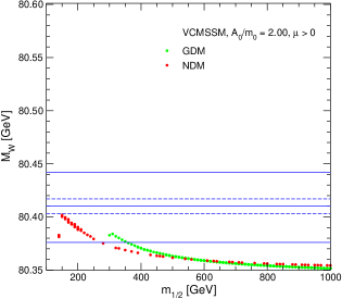
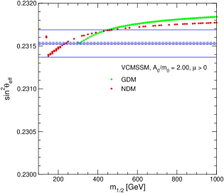
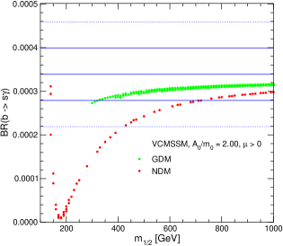
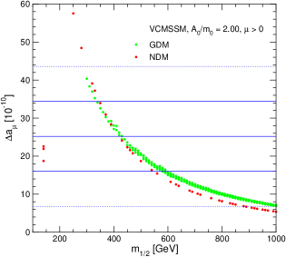
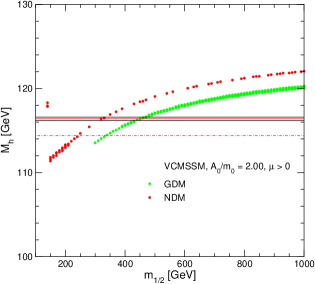
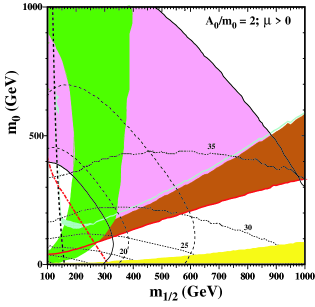
\begin{picture}(0.0,0.0) \put(0.0,0.0){} \put(0.0,0.0){} \put(0.0,0.0){} \put(0.0,0.0){} \put(0.0,0.0){} \put(0.0,0.0){} \put(0.0,0.0){} \put(0.0,0.0){} \end{picture}

Figure 12: Results as functions of $m_{1/2}$ along the VCMSSM WMAP strip for neutralino dark matter when $A_{0}/m_{0}=2$, for (a) $M_{W}$, (b) $\sin^{2}\theta_{\mathrm{eff}}$, (c) ${\rm BR}(b\to s\gamma)$, (d) $(g-2)_{\mu}$ and (e) $M_{h}$. Note the NDM points at low $m_{1/2}\sim 140\,\,\mathrm{GeV}$ that simultaneously fit very well ${\rm BR}(b\to s\gamma)$ and $(g-2)_{\mu}$. In panel (f) we display phenomenological constraints in the $(m_{1/2},m_{0})$ plane for the VCMSSM with $A_{0}/m_{0}=2$, including both the NDM WMAP strip (blue) and the GDM wedge (yellow). The regions disfavoured by $b\to s\gamma$ and favoured by $(g-2)_{\mu}$ are shaded green and pink (darker and lighter grey), respectively, the LEP Higgs constraint is a near-vertical (red) dashed line, and the (blue) dotted lines are contours of $\tan\beta$, as fixed by the VCMSSM vacuum conditions.

These behaviours can be understood by referring to panel (f) of Fig. 12, where the regions disfavoured by $b\to s\gamma$ and favoured by $(g-2)_{\mu}$ are shaded green and pink (darker and lighter grey), respectively. The shaded $(g-2)_{\mu}$ region represents a 2-$\sigma$ deviatation based on (14), while the dashed lines represent the region favoured at the 1-$\sigma$ level. The LEP Higgs constraint is a diagonal (red) dot-dashed line, while the near-vertical black dashed line shows the LEP constraint on the chargino mass. The pale (blue) shaded strip is favoured by WMAP for NDM. Below this strip, there is a red shaded region in which the LSP is the $\tilde{\tau}_{1}$ and therefore excluded. Below the $\tilde{\tau}_{1}$ LSP region, the gravitino is the LSP [9]. In the unshaded portion of the GDM region, the next-to-lightest supersymmetric particle (NLSP) will decay into a gravitino with unacceptable effects on the abundances of the light elements and is excluded by BBN [100, 9, 10, 101]. The pale (yellow) shaded wedge is favoured for gravitino dark matter as this region is allowed by BBN constraints. Finally, the black dotted curves labeled 20, 25, 30 and 35 correspond to the values of $\tan\beta$ required by the VCMSSM vacuum conditions. We see that the rapid-annihilation tail of the WMAP strip rises at low $m_{1/2}$ into a region allowed by $b\to s\gamma$, favoured by $(g-2)_{\mu}$ and tolerated by $M_{h}$. It is the synchronized non-monotonic behaviour of these last three observables that explains the similar non-monotonic behaviour of $\chi^{2}$ along the NDM WMAP strip in Fig. 11 and the low value of $\chi^{2}$ for the isolated rapid-annihilation point at $m_{1/2}\sim 140\,\,\mathrm{GeV}$ [24]. This is in fact the best overall fit point in this VCMSSM scenario, as seen in Fig. 11.

The preferred ranges of $m_{1/2}$ seen in Fig. 11 correspond, through the VCMSSM vacuum conditions, to preferred ranges in $\tan\beta$. As seen in Fig. 13, these increase with the chosen value of $A_{0}/m_{0}$, as does the correlation with $m_{1/2}$. For $A_{0}/m_{0}=0$ (top left panel), $\tan\beta\sim 7$, increasing to $\tan\beta\sim 10,15,32$ for $A_{0}/m_{0}=0.75,3-\sqrt{3},3$, respectively. In the last case, descending the VCMSSM WMAP strip to lower $m_{1/2}$, whereas we see that $\chi^{2}$ exceeds 10 for $m_{1/2}<350\,\,\mathrm{GeV}$, we see again the isolated dark (red) rapid-annihilation points with $m_{1/2}\sim 140\,\,\mathrm{GeV}$ [24], which have relatively large $\tan\beta\sim 37$.

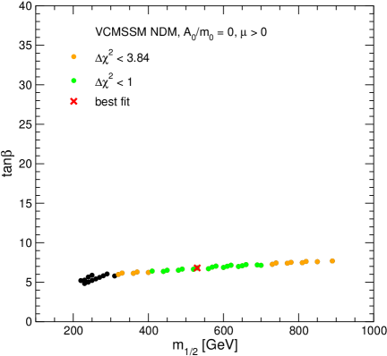
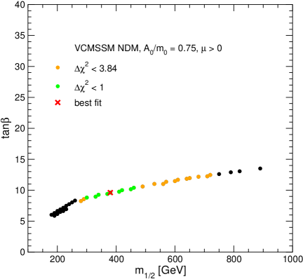
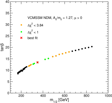
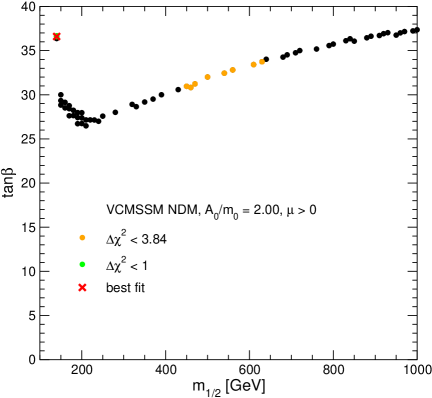
\begin{picture}(0.0,0.0) \put(0.0,0.0){} \put(0.0,0.0){} \put(0.0,0.0){} \put(0.0,0.0){} \put(0.0,0.0){} \put(0.0,0.0){} \end{picture}

Figure 13: Illustration of the preferred regions in the space of VCMSSM models for (a) $A_{0}=0$, (b) $A_{0}/m_{0}=0.75$, (c) $A_{0}/m_{0}=3-\sqrt{3}$ and (d) $A_{0}/m_{0}=2$. In each case, the red points show the $\chi^{2}$ minimum, the green points have $\Delta\chi^{2}<1$, the orange points have $\Delta\chi^{2}<3.84$, and the black points have larger $\chi^{2}$.

We conclude that the extra constraint imposed in the VCMSSM modifies but does not remove the preference found within the CMSSM for small $m_{1/2}$. Within the VCMSSM with neutralino dark matter, the minimum of $\chi^{2}$ usually occurs along the generic WMAP coannihilation strip at $m_{1/2}\sim 500\,\,\mathrm{GeV}$. However, when $A_{0}/m_{0}=2$, we find lower values of $\chi^{2}$ in the rapid light-Higgs annihilation region with $m_{1/2}\sim 140\,\,\mathrm{GeV}$. The preferred value of $\tan\beta$ varies between $\sim 7$ and $\sim 32$ on the generic WMAP strip, depending on the value of $A_{0}/m_{0}$, but $\tan\beta\sim 37$ in the light Higgs-pole annihilation region for $A_{0}/m_{0}=2$. These points offer prospects for a gluino discovery at the Tevatron: all the other preferred parameter sets offer good prospects for observing sparticles at the LHC and ILC(500).

6 GDM Analysis

The relation $A_{0}=B_{0}+m_{0}$ is just one of the further conditions on supersymmetry-breaking parameters that would be imposed in minimal supergravity (mSUGRA) models. The other is the equality between $m_{0}$ and the gravitino mass. So far, we have implicitly assumed that the gravitino is sufficiently heavy that the LSP is always the lightest neutralino $\tilde{\chi}^{0}_{1}$ and the cosmological constraints on gravitino decays are unimportant. However, this is not always the case in mSUGRA models. Indeed, in generic mSUGRA scenarios, as seen in the bottom right panel of Fig. 12, in addition to a WMAP strip where the $\tilde{\chi}^{0}_{1}$ is the LSP as we have assumed so far, there is a wedge of parameter space at lower values of $m_{0}$ (for given choices of $m_{1/2}$ and the other parameters), where the gravitino is the LSP. In this case, there are important astrophysical and cosmological constraints on the decays of the long-lived NLSP [100, 10, 101], which is generally the lighter stau $\tilde{\tau}_{1}$ in such mSUGRA scenarios .

Fig. 14 displays the $\chi^{2}$ function for a sampling of GDM scenarios obtained by applying the supplementary gravitino mass condition to VCMSSM models for $A_{0}/m_{0}=0,0.75,3-\sqrt{3}$ and 2, and scanning the GDM wedges at low $m_{0}$. These wedges are scanned via a series of points at fixed (small) $m_{0}$ and increasing $m_{1/2}$. We note that there is a marginal tendency for $\chi^{2}$ to increase with increasing $m_{0}$, though this is not as marked as the tendency to increase with $m_{1/2}$, and that the scan lines are more widely separated for the smaller values of $A_{0}$. Comparing Figs. 11 and 14, we see that lower $\chi^{2}$ values may be attained in the GDM cases. The third panel of Fig. 12 and last panel of Fig. 13 illustrate how this comes about in the case $A_{0}/m_{0}=2$: there is a large contribution to $\chi^{2}$ from $b\to s\gamma$ in the NDM for small $m_{1/2}$ that is absent in the GDM, which strongly prefers the combination of smaller $m_{0}$ and smaller $\tan\beta$ found in the GDM models .

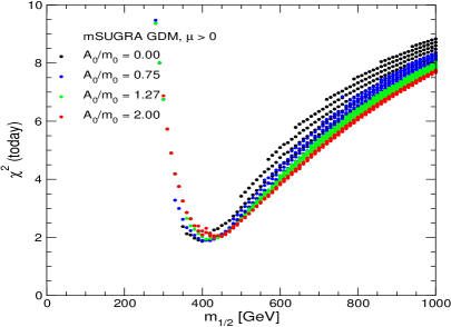
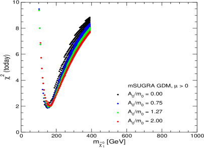
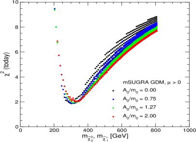
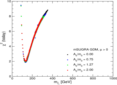
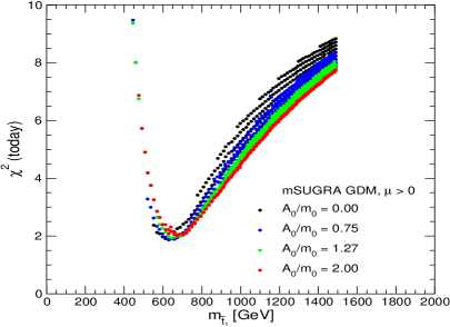
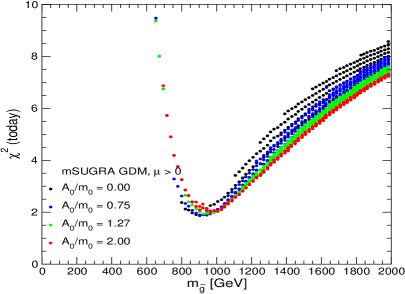
\begin{picture}(0.0,0.0) \put(0.0,0.0){} \put(0.0,0.0){} \put(0.0,0.0){} \put(0.0,0.0){} \put(0.0,0.0){} \put(0.0,0.0){} \put(0.0,0.0){} \put(0.0,0.0){} \put(0.0,0.0){} \put(0.0,0.0){} \end{picture}

Figure 14: The dependence of the $\chi^{2}$ function on $m_{1/2}$ for GDM scenarios with $A_{0}/m_{0}=0,0.75,3-\sqrt{3}$ and $2$, scanning the regions where the lighter stau $\tilde{\tau}_{1}$ is the NLSP, shown as a function of (a) $m_{1/2}$, (b) $m_{\tilde{\chi}^{0}_{1}}$, (c) $m_{\tilde{\chi}^{0}_{2}}$ and $m_{\tilde{\chi}^{\pm}_{1}}$, (d) $m_{\tilde{\tau}_{1}}$, (e) $m_{\tilde{t}_{1}}$, and (f) $m_{\tilde{g}}$.

As seen in Fig. 14, the global minimum of $\chi^{2}$ for all the VCMSSM GDM models with $A_{0}/m_{0}=0,0.75,3-\sqrt{3}$ and 2 is at $m_{1/2}\sim 450\,\,\mathrm{GeV}$. However, this minimum is not attained for GDM models with larger $m_{0}$, as they do not reach the low-$m_{1/2}$ tip of the GDM wedge seen, for example, in the last panel of Fig. 15. In general, we see in the different panels of Fig. 14 that, as in the CMSSM, there are good prospects for observing the $\tilde{g}$ and perhaps the $\tilde{t}_{1}$ at the LHC, and that the ILC(500) has good prospects for the $\tilde{\chi}^{0}_{1}$ and $\tilde{\tau}_{1}$, though these diminish for larger $m_{0}$. The ILC(1000), again, offers much better chances also for large $m_{0}$. We recall that, in these GDM scenarios, the $\tilde{\tau}_{1}$ is the NLSP, and that the $\tilde{\chi}^{0}_{1}$ is heavier. The $\tilde{\tau}_{1}$ decays into the gravitino and a $\tau$, and is metastable with a lifetime that may be measured in hours, days or weeks. Specialized detection strategies for the LHC were discussed in [25]: this scenario would offer exciting possibilities near the $\tilde{\tau}_{1}$ pair-production threshold at the ILC.

As discussed above, a feature of the class of GDM scenarios discussed here is that the required value of $\tan\beta$ increases with $m_{1/2}$. Therefore, the preference for relatively small $m_{1/2}$ discussed above maps into an analogous preference for moderate $\tan\beta$, as shown in Fig. 15. The different panels are for the four choices $A_{0}/m_{0}=0,0.75,3-\sqrt{3}$ and 2. In each case, the red point indicates the minimum of the $\chi^{2}$ function, the green points have $\Delta\chi^{2}<1$ corresponding to the 68 % confidence level, the orange points have $\Delta\chi^{2}<3.84$ corresponding to the 95 % confidence level, and the black points have larger $\Delta\chi^{2}$. We see that, at the 95 % confidence level

$$300\,\,\mathrm{GeV}\;\raisebox{-3.00003pt}{$\stackrel{{\scriptstyle\displaystyle<}}{{\sim}}$}\;m_{1/2}\;\raisebox{-3.00003pt}{$\stackrel{{\scriptstyle\displaystyle<}}{{\sim}}$}\;800\,\,\mathrm{GeV},\quad 15\;\raisebox{-3.00003pt}{$\stackrel{{\scriptstyle\displaystyle<}}{{\sim}}$}\;\tan\beta\;\raisebox{-3.00003pt}{$\stackrel{{\scriptstyle\displaystyle<}}{{\sim}}$}\;27$$ (23)

in this mSUGRA class of GDM models.

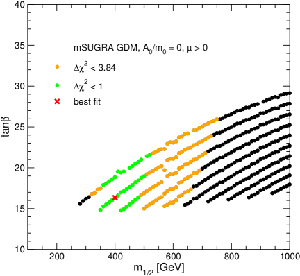
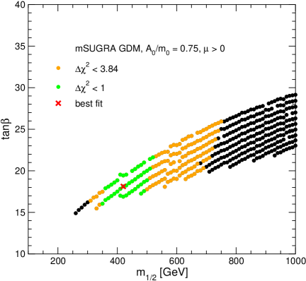
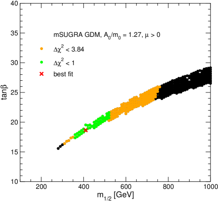
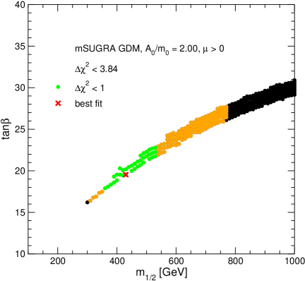
\begin{picture}(0.0,0.0) \put(0.0,0.0){} \put(0.0,0.0){} \put(0.0,0.0){} \put(0.0,0.0){} \put(0.0,0.0){} \put(0.0,0.0){} \end{picture}

Figure 15: Illustration of the preferred regions in the space of mSUGRA-motivated GDM models for (a) $A_{0}=0$, (b) $A_{0}/m_{0}=0.75$, (c) $A_{0}/m_{0}=3-\sqrt{3}$ and (d) $A_{0}/m_{0}=2$. In each case, the red points show the $\chi^{2}$ minimum, the green points have $\Delta\chi^{2}<1$, the orange points have $\Delta\chi^{2}<3.84$, and the black points have larger $\chi^{2}$.

7 Conclusions

Precision electroweak data and rare processes have some sensitivity to the loop corrections that might be induced by supersymmetric particles. As we discussed previously in the context of the CMSSM [1, 2], present data exhibit some preference for a relatively low scale of soft supersymmetry breaking: $m_{1/2}\sim 300\ldots 600\,\,\mathrm{GeV}$. This preference is largely driven by $(g-2)_{\mu}$, with some support from measurements of $M_{W}$ and $\sin^{2}\theta_{\mathrm{eff}}$. In this paper we have re-evaluated this preference, in the light of new measurements of $m_{t}$ and $M_{W}$, and treating more completely the information provided by the bound from the LEP direct searches for the Higgs boson. The preference for $m_{1/2}\sim 300\ldots 600\,\,\mathrm{GeV}$ is maintained in the CMSSM, and also in other scenarios that implement different assumptions for soft supersymmetry breaking. These include the less constrained NUHM models in which the soft supersymmetry-breaking scalar masses for the two Higgs multiplets are treated as free parameters as well as more constrained VCMSSM models in which the soft trilinear and bilinear supersymmetry-breaking parameters are related. The same preference is also maintained in GDM models motivated by mSUGRA, where the LSP is the gravitino instead of being a neutralino as assumed in the other scenarios.

Whilst $m_{1/2}$ is quite constrained in our analysis, there are NUHM scenarios in which $m_{0}$ could be considerably larger than the corresponding values in the CMSSM, and significant variations in $\mu$ and $M_{A}$ are also possible. Within the CMSSM and NUHM, we find no preference for any particular range of $\tan\beta$, but the preferred values of $m_{1/2}$ in the VCMSSM and GDM scenarios studied here correspond to intermediate values of $\tan\beta\sim 15$ to 30.

The ranges of $m_{1/2}$ that are preferred would correspond to gluinos and other sparticles being light enough to be produced readily at the LHC. Many sparticles would also be observable at the ILC in the preferred CMSSM, VCMSSM and GDM scenarios considered, but the larger values of $m_{0}$ allowed in some of the NUHM scenarios would reduce the number of sparticle species detectable at the ILC, at least when operated at 500 GeV, whereas the ILC at $\sqrt{s}=1000\,\,\mathrm{GeV}$ covers the full range for some sparticle species. There are also prospects for detecting supersymmetry at the Tevatron in some special VCMSSM models with neutralino dark matter.

We re-emphasize that our analysis depends in considerable part on the estimate of the Standard Model contribution to $(g-2)_{\mu}$ based on $e^{+}e^{-}$ annihilation data, that we assume in this paper. Our conclusions would be weakened if the Standard Model calculation were to be based on $\tau$ decay data. Additional $e^{+}e^{-}$ data are now coming available, and it will be important to take into account whatever update of the Standard Model contribution to $(g-2)_{\mu}$ they may provide. However, the measurement of $M_{W}$ is increasing in importance, particularly in the light of the recent evolution of the preferred value of $m_{t}$. Future measurements of $M_{W}$ and $m_{t}$ at the Tevatron will be particularly important in this regard.

Acknowledgements

S.H. and G.W. thank P. Bechtle and K. Desch for detailed explanations on how to obtain $\chi^{2}$ values from the SM Higgs boson searches at LEP. We thank A. Read for providing the corresponding $CL_{s}$ numbers. The work of S.H. was partially supported by CICYT (grant FPA2004-02948) and DGIID-DGA (grant 2005-E24/2). The work of K.A.O. was partially supported by DOE grant DE-FG02-94ER-40823.

References

- [1] J. Ellis, S. Heinemeyer, K. Olive and G. Weiglein, JHEP 0502 013, hep-ph/0411216.
- [2] J. Ellis, S. Heinemeyer, K. Olive and G. Weiglein, hep-ph/0508169.
- [3] H. Nilles, Phys. Rep. 110 (1984) 1.
-
[4]
H. Haber and G. Kane,
Phys. Rep. 117, (1985) 75;
R. Barbieri, Riv. Nuovo Cim. 11, (1988) 1. -
[5]
V. Berezinsky, A. Bottino, J. Ellis, N. Fornengo,
G. Mignola and S. Scopel,
Astropart. Phys. 5 (1996) 1,
hep-ph/9508249;
M. Drees, M. Nojiri, D. Roy and Y. Yamada, Phys. Rev. D 56 (1997) 276, [Erratum-ibid. D 64 (1997) 039901], hep-ph/9701219;
M. Drees, Y. Kim, M. Nojiri, D. Toya, K. Hasuko and T. Kobayashi, Phys. Rev. D 63 (2001) 035008, hep-ph/0007202;
P. Nath and R. Arnowitt, Phys. Rev. D 56 (1997) 2820, hep-ph/9701301;
A. Bottino, F. Donato, N. Fornengo and S. Scopel, Phys. Rev. D 63 (2001) 125003, hep-ph/0010203;
S. Profumo, Phys. Rev. D 68 (2003) 015006, hep-ph/0304071;
D. Cerdeno and C. Munoz, JHEP 0410 (2004) 015, hep-ph/0405057;
H. Baer, A. Mustafayev, S. Profumo, A. Belyaev and X. Tata, JHEP 0507 (2005) 065, hep-ph/0504001. -
[6]
J. Ellis, K. Olive and Y. Santoso,
Phys. Lett. B 539 (2002) 107,
hep-ph/0204192;
J. Ellis, T. Falk, K. Olive and Y. Santoso, Nucl. Phys. B 652 (2003) 259, hep-ph/0210205. - [7] J. Ellis, K. Olive, Y. Santoso and V. Spanos, Phys. Lett. B 573 (2003) 162, hep-ph/0305212; Phys. Rev. D 70 (2004) 055005, hep-ph/0405110.
-
[8]
J. Ellis, J. Kim and D. Nanopoulos,
Phys. Lett. B 145 (1984) 181;
T. Moroi, H. Murayama and M. Yamaguchi, Phys. Lett. 303 (1993) 289;
J. Ellis, D. Nanopoulos, K. Olive and S. Rey, Astropart. Phys. 4 (1996) 371, hep-ph/9505438;
M. Bolz, W. Buchmüller and M. Plümacher, Phys. Lett. B 443 (1998) 209, hep-ph/9809381;
T. Gherghetta, G. Giudice and A. Riotto, Phys. Lett. B 446 (1999) 28, hep-ph/9808401;
T. Asaka, K. Hamaguchi and K. Suzuki, Phys. Lett. B 490 (2000) 136, hep-ph/0005136;
M. Fujii and T. Yanagida, Phys. Rev. D 66 (2002) 123515, hep-ph/0207339; Phys. Lett. B 549 (2002) 273, hep-ph/0208191;
M. Bolz, A. Brandenburg and W. Buchmüller, Nucl. Phys. B 606 (2001) 518, hep-ph/0012052;
W. Buchmüller, K. Hamaguchi and M. Ratz, Phys. Lett. B 574 (2003) 156, hep-ph/0307181. - [9] J. Ellis, K. Olive, Y. Santoso and V. Spanos, Phys. Lett. B 588 (2004) 7, hep-ph/0312262.
- [10] J. Ellis, K. Olive and E. Vangioni, Phys. Lett. B 619 (2005) 30, astro-ph/0503023.
-
[11]
J. Feng, S. Su and F. Takayama,
Phys. Rev. D 70 (2004) 075019,
hep-ph/0404231;
Phys. Rev. D 70 (2004) 063514,
hep-ph/0404198;
J. Feng, A. Rajaraman and F. Takayama, Phys. Rev. Lett. 91 (2003) 011302, hep-ph/0302215. -
[12]
T. Appelquist and J. Carazzone,
Phys. Rev. D 11 (1975) 2856;
A. Dobado, M. Herrero and S. Peñaranda, Eur. Phys. J. C 7 (1999) 313, hep-ph/9710313, Eur. Phys. J. C 12 (2000) 673, hep-ph/9903211; Eur. Phys. J. C 17 (2000) 487, hep-ph/0002134. - [13] S. Heinemeyer, W. Hollik and G. Weiglein, Phys. Rept. 425 (2006) 265, hep-ph/0412214.
- [14] J. Ellis, K. Olive, Y. Santoso and V. Spanos, Phys. Lett. B 565 (2003) 176, hep-ph/0303043.
-
[15]
H. Baer and C. Balazs,
JCAP 0305 (2003) 006,
hep-ph/0303114;
A. Lahanas and D. Nanopoulos, Phys. Lett. B 568 (2003) 55, hep-ph/0303130;
U. Chattopadhyay, A. Corsetti and P. Nath, Phys. Rev. D 68 (2003) 035005, hep-ph/0303201;
C. Munoz, hep-ph/0309346. -
[16]
C. Bennett et al.,
Astrophys. J. Suppl. 148 (2003) 1,
astro-ph/0302207;
D. Spergel et al. [WMAP Collaboration], Astrophys. J. Suppl. 148 (2003) 175, astro-ph/0302209. -
[17]
V. Abazov et al. [D0 Collaboration],
Nature 429 (2004) 638,
hep-ex/0406031;
P. Azzi et al. [CDF Collaboration, D0 Collaboration], hep-ex/0404010. - [18] CDF Collaboration, D0 Collaboration and Tevatron Electroweak Working Group, hep-ex/0507091.
- [19] LEP Higgs working group, Phys. Lett. B 565 (2003) 61, hep-ex/0306033.
- [20] LEP Higgs working group, hep-ex/0107030; hep-ex/0107031; LHWG-Note 2004-01, see: lephiggs.web.cern.ch/LEPHIGGS/papers/ .
-
[21]
J. Ellis, K. Olive, Y. Santoso and V. Spanos,
Phys. Rev. D 69 (2004) 095004,
hep-ph/0310356;
B. Allanach and C. Lester, Phys. Rev. D 73 (2006) 015013, hep-ph/0507283;
B. Allanach, hep-ph/0601089;
R. de Austri, R. Trotta and L. Roszkowski, hep-ph/0602028. - [22] J. Aguilar-Saavedra et al., hep-ph/0511344.
-
[23]
J. Polonyi,
Budapest preprint KFKI-1977-93 (1977);
R. Barbieri, S. Ferrara and C. Savoy, Phys. Lett. B 119 (1982) 343. - [24] A. Djouadi, M. Drees and J. Kneur, Phys. Lett. B 624 (2005) 60, hep-ph/0504090.
-
[25]
K. Hamaguchi, Y. Kuno, T. Nakaya and M. Nojiri,
Phys. Rev. D 70 (2004) 115007,
hep-ph/0409248;
J. Feng and B. Smith, Phys. Rev. D 71 (2005) 015004 [Erratum-ibid. D 71 (2005) 0109904], hep-ph/0409278;
A. De Roeck, J. Ellis, F. Gianotti, F. Moortgat, K. Olive and L. Pape, hep-ph/0508198. -
[26]
B. Allanach, G. Belanger, F. Boudjema and A. Pukhov,
JHEP 0412 (2004) 020,
hep-ph/0410091;
H. Baer, J. Ferrandis, S. Kraml and W. Porod, hep-ph/0511123. -
[27]
A. Sirlin,
Phys. Rev. D 22 (1980) 971;
W. Marciano and A. Sirlin, Phys. Rev. D 22 (1980) 2695. - [28] P. Chankowski, A. Dabelstein, W. Hollik, W. Mösle, S. Pokorski and J. Rosiek, Nucl. Phys. B 417 (1994) 101.
- [29] D. Garcia and J. Solà, Mod. Phys. Lett. A 9 (1994) 211.
-
[30]
A. Djouadi and C. Verzegnassi,
Phys. Lett. B 195 (1987) 265;
A. Djouadi, Nuovo Cim. A 100 (1988) 357. -
[31]
B. Kniehl,
Nucl. Phys. B 347 (1990) 89;
F. Halzen and B. Kniehl, Nucl. Phys. B 353 (1991) 567;
B. Kniehl and A. Sirlin, Nucl. Phys. B 371 (1992) 141; Phys. Rev. D 47 (1993) 883. -
[32]
K. Chetyrkin, J.H. Kühn and M. Steinhauser,
Phys. Rev. Lett. 75 (1995) 3394,
hep-ph/9504413;
L. Avdeev et al., Phys. Lett. B 336 (1994) 560, [Erratum-ibid. B 349 (1995) 597], hep-ph/9406363. - [33] K. Chetyrkin, J.H. Kühn and M. Steinhauser, Nucl. Phys. B 482 (1996) 213, hep-ph/9606230.
- [34] A. Djouadi, P. Gambino, S. Heinemeyer, W. Hollik, C. Jünger and G. Weiglein, Phys. Rev. Lett. 78 (1997) 3626, hep-ph/9612363; Phys. Rev. D 57 (1998) 4179, hep-ph/9710438.
- [35] S. Heinemeyer and G. Weiglein, JHEP 0210 (2002) 072, hep-ph/0209305; hep-ph/0301062.
- [36] J. Haestier, S. Heinemeyer, D. Stöckinger and G. Weiglein, JHEP 0512 (2005) 027, hep-ph/0508139; hep-ph/0506259.
- [37] S. Heinemeyer, W. Hollik, D. Stöckinger, A.M. Weber and G. Weiglein, hep-ph/0604147.
- [38] S. Heinemeyer and G. Weiglein, hep-ph/0508168.
-
[39]
[The ALEPH, DELPHI, L3, OPAL, SLD Collaborations,
the LEP Electroweak Working Group,
the SLD Electroweak and Heavy Flavour Groups],
hep-ex/0509008;
[The ALEPH, DELPHI, L3 and OPAL Collaborations, the LEP Electroweak Working Group], hep-ex/0511027. -
[40]
M. Grünewald,
hep-ex/0304023; for an update, see:
C. Diaconu, talk given at the Lepton-Photon 2005 Symposium, Uppsala, Sweden, June 2005: lp2005.tsl.uu.se/lp2005/LP2005/programme/presentationer/morning/
diaconu.pdf; see also: lepewwg.web.cern.ch/LEPEWWG/Welcome.html. - [41] A. Czarnecki and W. Marciano, Phys. Rev. D 64 (2001) 013014, hep-ph/0102122.
-
[42]
M. Knecht,
hep-ph/0307239;
M. Passera, hep-ph/0509372. - [43] T. Kinoshita and M. Nio, hep-ph/0402206.
- [44] M. Davier, S. Eidelman, A. Höcker and Z. Zhang, Eur. Phys. J. C 31 (2003) 503, hep-ph/0308213.
- [45] K. Hagiwara, A. Martin, D. Nomura and T. Teubner, Phys. Rev. D 69 (2004) 093003, hep-ph/0312250.
- [46] S. Ghozzi and F. Jegerlehner, Phys. Lett. B 583 (2004) 222, hep-ph/0310181.
- [47] J. de Troconiz and F. Yndurain, hep-ph/0402285.
- [48] J. Bijnens, E. Pallante and J. Prades, Phys. Rev. Lett. 75 (1995) 1447 [Erratum-ibid. 75 (1995) 3781], hep-ph/9505251; Nucl. Phys. B 474 (1996) 379, hep-ph/9511388; Nucl. Phys. B 626 (2002) 410, hep-ph/0112255.
-
[49]
M. Hayakawa, T. Kinoshita and A. Sanda,
Phys. Rev. D 54 (1996) 3137,
hep-ph/9601310;
M. Hayakawa and T. Kinoshita, Phys. Rev. D 57 (1998) 465 [Erratum-ibid. D 66 (2002) 019902], hep-ph/9708227; hep-ph/0112102. -
[50]
M. Knecht and A. Nyffeler,
Phys. Rev. D 65 (2002) 073034,
hep-ph/0111058;
M. Knecht, A. Nyffeler, M. Perrottet and E. De Rafael, Phys. Rev. Lett. 88 (2002) 071802, hep-ph/0111059;
I. Blokland, A. Czarnecki and K. Melnikov, Phys. Rev. Lett. 88 (2002) 071803, hep-ph/0112117;
M. Ramsey-Musolf and M. Wise, Phys. Rev. Lett. 89 (2002) 041601, hep-ph/0201297;
J. Kühn, A. Onishchenko, A. Pivovarov and O. Veretin, Phys. Rev. D 68 (2003) 033018, hep-ph/0301151. - [51] K. Melnikov and A. Vainshtein, Phys. Rev. D 70 (2004) 113006, hep-ph/0312226.
- [52] A. Hocker, hep-ph/0410081.
- [53] A. Aloisio et al. [KLOE Collaboration], hep-ex/0407048.
- [54] R. Akhmetshin et al. [CMD-2 Collaboration], Phys. Lett. B 578 (2004) 285, hep-ex/0308008.
- [55] M. Achasov et al. [SND Collaboration], hep-ex/0506076.
- [56] G. Bennett et al., [The Muon g-2 Collaboration], Phys. Rev. Lett. 92 (2004) 161802, hep-ex/0401008.
- [57] G. Bennett et al., [The Muon g-2 Collaboration], hep-ex/0602035.
- [58] T. Moroi, Phys. Rev. D 53 (1996) 6565 [Erratum-ibid. D 56 (1997) 4424], hep-ph/9512396.
- [59] G. Degrassi and G. Giudice, Phys. Rev. D 58 (1998) 053007, hep-ph/9803384.
- [60] S. Heinemeyer, D. Stöckinger and G. Weiglein, Nucl. Phys. B 690 (2004) 62, hep-ph/0312264.
- [61] S. Heinemeyer, D. Stöckinger and G. Weiglein, Nucl. Phys. B 699 (2004) 103, hep-ph/0405255.
- [62] H. Asatrian, A. Hovhannisyan, C. Greub, T. Hurth and V. Poghosyan, hep-ph/0512097.
-
[63]
K. Adel and Y. Yao,
Phys. Rev. D 49 (1994) 4945,
hep-ph/9308349;
C. Greub, T. Hurth and D. Wyler, Phys. Lett. B 380 (1996) 385, hep-ph/9602281; Phys. Rev. D 54 (1996) 3350, hep-ph/9603404;
A. Ali, talk given at ICHEP04, Beijing, August 2004, to appear in the proceedings, see: ichep04.ihep.ac.cn/db/paper.php . - [64] P. Gambino and M. Misiak, Nucl. Phys. B 611 (2001) 338, hep-ph/0104034.
- [65] K. Chetyrkin, M. Misiak and M. Münz, Phys. Lett. B 400, (1997) 206, [Erratum-ibid. B 425 (1998) 414] hep-ph/9612313.
- [66] T. Hurth, E. Lunghi and W. Porod, Nucl. Phys. B 704 (2005) 56, hep-ph/0312260.
- [67] M. Neubert, Eur. Phys. J. C 40 (2005) 165, hep-ph/0408179.
-
[68]
R. Barate et al. [ALEPH Collaboration],
Phys. Lett. B 429 (1998) 169;
S. Chen et al. [CLEO Collaboration], Phys. Rev. Lett. 87 (2001) 251807, hep-ex/0108032;
P. Koppenburg et al. [Belle Collaboration], Phys. Rev. Lett. 93 (2004) 061803, hep-ex/0403004;
K. Abe et al. [Belle Collaboration], Phys. Lett. B 511 (2001) 151, hep-ex/0103042;
B. Aubert et al. [BABAR Collaboration], hep-ex/0207074; hep-ex/0207076;
see also www.slac.stanford.edu/xorg/hfag/ . - [69] G. Belanger, F. Boudjema, A. Pukhov and A. Semenov, Comput. Phys. Comm. 149 (2002) 103, hep-ph/0112278; hep-ph/0405253.
- [70] C. Degrassi, P. Gambino and G. Giudice, JHEP 0012 (2000) 009, hep-ph/0009337.
-
[71]
P. Cho, M. Misiak and D. Wyler,
Phys. Rev. D 54, 3329 (1996),
hep-ph/9601360;
A. Kagan and M. Neubert, Eur. Phys. J. C 7 (1999) 5, hep-ph/9805303;
A. Ali, E. Lunghi, C. Greub and G. Hiller, Phys. Rev. D 66 (2002) 034002, hep-ph/0112300;
G. Hiller and F. Krüger, Phys. Rev. D 69 (2004) 074020, hep-ph/0310219;
M. Carena, D. Garcia, U. Nierste and C. Wagner, Phys. Lett. B 499 (2001) 141, hep-ph/0010003;
D. Demir and K. Olive, Phys. Rev. D 65 (2002) 034007, hep-ph/0107329;
T. Hurth, hep-ph/0212304. -
[72]
F. Abe et al. [CDF Collaboration],
Phys. Rev. D 57 (1998) 3811;
D. Acosta et al. [CDF Collaboration], Phys. Rev. Lett. 93 (2004) 032001, hep-ex/0403032;
V. Abazov et al. [D0 Collaboration], Phys. Rev. Lett. 94 (2005) 071802, hep-ex/0410039;
D0 Collaboration, D0note, 4733-CONF, see:
www-d0.fnal.gov/Run2Physics/WWW/results/prelim/B/B21/B21.pdf ;
M. Herndon [CDF and D0 Collaborations], FERMILAB-CONF-04-391-E. Published Proceedings 32nd International Conference on High-Energy Physics (ICHEP 04), Beijing, China, August 16-22, 2004;
CDF Collaboration, CDF note 7670, see:
www-cdf.fnal.gov/physics/new/bottom/050407.blessed-bsmumu . -
[73]
A. Dedes, H. Dreiner and U. Nierste,
Phys. Rev. Lett. 87 (2001) 251804,
hep-ph/0108037;
R. Arnowitt, B. Dutta, T. Kamon and M. Tanaka, Phys. Lett. B 538 (2002) 121, hep-ph/0203069;
S. Baek, P. Ko and W. Song, Phys. Rev. Lett. 89 (2002) 271801, hep-ph/0205259;
C. Huang and X. Wu, Nucl. Phys. B 657 (2003) 304, hep-ph/0212220;
S. Baek, Y. Kim and P. Ko, JHEP 0502 (2005) 067, hep-ph/0406033;
H. Baer, C. Balazs, A. Belyaev, J. Mizukoshi, X. Tata and Y. Wang, JHEP 0207 (2002) 050, hep-ph/0205325. - [74] J. Ellis, K. Olive and V. Spanos, Phys. Lett. B 624 (2005) 47, hep-ph/0504196.
- [75] J. Ellis, K. Olive, Y. Santoso and V. Spanos, hep-ph/0603136.
- [76] S. Heinemeyer, W. Hollik and G. Weiglein, Comp. Phys. Comm. 124 2000 76, hep-ph/9812320; Eur. Phys. J. C 9 (1999) 343, hep-ph/9812472. The codes are accessible via www.feynhiggs.de .
-
[77]
S. Heinemeyer,
hep-ph/0407244;
T. Hahn, S. Heinemeyer, W. Hollik and G. Weiglein, hep-ph/0507009;
T. Hahn, M. Frank, S. Heinemeyer, W. Hollik, H. Rzehak and G. Weiglein, in preparation. -
[78]
Y. Okada, M. Yamaguchi, T. Yanagida,
Prog. Theor. Phys. 85 (1991) 1;
J. Ellis, G. Ridolfi, F. Zwirner, Phys. Lett. B 257 (1991) 83;
H. Haber, R. Hempfling, Phys. Rev. Lett. 66 (1991) 1815. - [79] P. Chankowski, S. Pokorski, J. Rosiek, Phys. Lett. B 286 (1992) 307; Nucl. Phys. B 423 (1994) 437, hep-ph/9303309.
- [80] A. Dabelstein, Nucl. Phys. B 456 (1995) 25, hep-ph/9503443; Z. Phys. C 67 (1995) 495, hep-ph/9409375.
- [81] G. Degrassi, S. Heinemeyer, W. Hollik, P. Slavich, G. Weiglein, Eur. Phys. J. C 28 (2003) 133, hep-ph/0212020.
-
[82]
M. Carena, D. Garcia, U. Nierste and C. Wagner,
Nucl. Phys. B 577 (2000) 577,
hep-ph/9912516;
H. Eberl, K. Hidaka, S. Kraml, W. Majerotto and Y. Yamada, Phys. Rev. D 62 (2000) 055006, hep-ph/9912463. -
[83]
T. Banks,
Nucl. Phys. B 303 (1988) 172;
L. Hall, R. Rattazzi and U. Sarid, Phys. Rev. D 50 (1994) 7048, hep-ph/9306309;
R. Hempfling, Phys. Rev. D 49 (1994) 6168;
M. Carena, M. Olechowski, S. Pokorski and C. Wagner, Nucl. Phys. B 426 (1994) 269, hep-ph/9402253. - [84] G. Degrassi, A. Dedes, P. Slavich, Nucl. Phys. B 672 (2003) 144, hep-ph/0305127.
-
[85]
S. Martin,
Phys. Rev. D 65 (2002) 116003,
hep-ph/0111209;
Phys. Rev. D 66 (2002) 096001,
hep-ph/0206136;
Phys. Rev. D 67 (2003) 095012,
hep-ph/0211366;
Phys. Rev. D 68 075002 (2003),
hep-ph/0307101;
Phys. Rev. D 70 (2004) 016005,
hep-ph/0312092;
Phys. Rev. D 71 (2005) 016012,
hep-ph/0405022;
Phys. Rev. D 71 (2005) 116004,
hep-ph/0502168;
S. Martin and D. Robertson, hep-ph/0501132. - [86] S. Heinemeyer, W. Hollik, H. Rzehak and G. Weiglein, Eur. Phys. J. C 39 (2005) 465, hep-ph/0411114; hep-ph/0506254.
- [87] B. Allanach, A. Djouadi, J. Kneur, W. Porod and P. Slavich, JHEP 0409 (2004) 044, hep-ph/0406166.
- [88] S. Ambrosanio, A. Dedes, S. Heinemeyer, S. Su and G. Weiglein, Nucl. Phys. B 624 (2001) 3, hep-ph/0106255.
- [89] J. Ellis, S. Heinemeyer, K. Olive and G. Weiglein, Phys. Lett. B 515 (2001) 348, hep-ph/0105061.
- [90] S. Eidelman et al. [Particle Data Group], Phys. Lett. B 592 (2004) 1.
- [91] S. Heinemeyer, W. Hollik and G. Weiglein, JHEP 0006 (2000) 009, hep-ph/9909540.
-
[92]
J. Feng, K. Matchev and T. Moroi,
Phys. Rev. Lett. 84 (2000) 2322,
hep-ph/9908309;
Phys. Rev. D 61 (2000) 075005,
hep-ph/9909334;
J. Feng, K. Matchev and F. Wilczek, Phys. Lett. B 482 (2000) 388, hep-ph/0004043;
J. Feng and K. Matchev, Phys. Rev. D 63 (2001) 095003, hep-ph/0011356. - [93] B. Allanach et al., Eur. Phys. J. C 25 (2002) 113, hep-ph/0202233.
-
[94]
M. Battaglia et al.,
Eur. Phys. J. C 22, 535 (2001),
hep-ph/0106204;
M. Battaglia, A. De Roeck, J. Ellis, F. Gianotti, K. Olive and L. Pape, Eur. Phys. J. C 33 (2004) 273, hep-ph/0306219. - [95] G. Weiglein et al. [LHC / ILC Study Group], to appear in Phys. Rep., hep-ph/0410364.
- [96] Tevatron Electroweak Working Group, hep-ex/0603039.
- [97] J. Ellis, S. Heinemeyer, K. Olive and G. Weiglein, JHEP 0301 (2003) 006, hep-ph/0211206.
- [98] M. Drees and M. Nojiri, Nucl. Phys. B 369 (1992) 54.
- [99] A. Dedes, S. Heinemeyer, S. Su and G. Weiglein, Nucl. Phys. B 674 (2003) 271, hep-ph/0302174.
- [100] R. Cyburt, J. Ellis, B. Fields and K. Olive, Phys. Rev. D 67 (2003) 103521, astro-ph/0211258.
-
[101]
K. Kohri, T. Moroi and A. Yotsuyanagi,
hep-ph/0507245 and references therein;
D. Cerdeno, K. Choi, K. Jedamzik, L. Roszkowski and R. Ruiz de Austri, hep-ph/0509275.