Absence of the London limit for the first-order phase transition to a color superconductor

Abstract

We study the effects of gauge-field fluctuations on the free energy of a homogeneous color superconductor in the color-flavor-locked (CFL) phase. Gluonic fluctuations induce a strong first-order phase transition, in contrast to electronic superconductors where this transition is weakly first order. The critical temperature for this transition is larger than the one corresponding to the diquark pairing instability. The physical reason is that the gluonic Meissner masses suppress long-wavelength fluctuations as compared to the normal conducting phase where gluons are massless, which stabilizes the superconducting phase. In weak coupling, we analytically compute the temperatures associated with the limits of metastability of the normal and superconducting phases, as well as the latent heat associated with the first-order phase transition. We then extrapolate our results to intermediate densities and numerically evaluate the temperature of the fluctuation-induced first-order phase transition, as well as the discontinuity of the diquark condensate at the critical point. We find that the London limit of magnetic interactions is absent in color superconductivity.

I Introduction

It was suggested a long time ago that quark matter might exist within the central regions of superdense stars itoh . Since Quantum Chromodynamics (QCD) is an asymptotically free theory asymptfree , it was argued that the extremely compressed matter found in neutron stars consists of quarks rather than of hadrons and that realistic calculations in the framework of QCD become possible collinsperry . At high baryon densities and sufficiently low temperatures, however, a phase transition between normal and color-superconducting quark matter is expected love ; reviews ; dirkreview ; recentreviews . Therefore, color superconductivity (CSC) may be relevant to explain several important aspects of the highly compressed matter present in compact stars, e.g., the cooling rates astrostuff , and the rotational properties of stars madsen . Nevertheless, trustworthy perturbative calculations can only be performed for ultra-high chemical potentials, $\mu\gg\Lambda_{\rm QCD}$. The weak-coupling expansion of the temperature for the diquark pairing instability reads son ; gapTc

$$\ln\frac{T_{c}}{\mu}=-\frac{3\pi^{2}}{\sqrt{2}g}+\ln\frac{2048\sqrt{2}\pi^{3}}{9\sqrt{3}g^{5}}+\gamma-\frac{\pi^{2}+4}{8}+O(g)\;,$$ (1)

where $g$ is QCD running coupling constant at the chemical potential $\mu$, and $\gamma$ is the Euler-Mascheroni constant. The energy gap at $T=0$ in the CFL phase is dirkreview

$$\Delta(0)=2^{-\frac{1}{3}}\pi e^{-\gamma}\,T_{c}\;.$$ (2)

It follows from the Ginzburg-Landau (GL) theory of CSC in weak coupling that the phase transition is of second order at $T_{c}$ and the GL parameter is gia

$$\kappa=\sqrt{\frac{72\pi^{3}}{7\zeta(3)\alpha_{s}}}\,\frac{T_{c}}{\mu}\;,$$ (3)

with $\alpha_{s}=g^{2}/(4\pi)$. When $g\rightarrow 0$ then $\kappa\rightarrow 0$ and, therefore, the CFL color superconductor is of extreme type I.

It is well known in the context of electronic superconductors that gauge-field fluctuations change the second-order phase transition into a first-order transition ma . However, the strength of this first-order transition is sensitive to the relationship among the three length scales that are involved: the coherence length near the transition, $\xi$, the magnetic penetration depth near the transition, $\lambda$, and the coherence length at $T=0$, $\xi_{0}\sim\frac{1}{T_{c}}$. A superconductor with $\lambda\gg\xi_{0}$ is said to be in the London limit. In this case, the coupling between the gauge field and the order parameter is approximately local. The opposite case, $\lambda\ll\xi_{0}$, corresponds to the Pippard limit and the coupling becomes highly nonlocal lif . For a type-I electronic superconductor the Pippard limit is always realized at $T=0$. As the temperature is raised towards the transition to normal quark matter, the penetration depth increases and so does the ratio $\lambda/\xi_{0}$. A crossover from the Pippard limit to the London limit would be expected if the transition is of second order. How does the first-order phase transition induced by gauge-field fluctuations change this scenario? Are both limits still realized? In the case of known electronic superconductors of type I, the first-order phase transition is sufficiently weak to warrant a crossover between Pippard and London limits, which has been indeed observed experimentally for strong type-I materials like aluminum bonalde . However, the situation is completely different for a color superconductor. It was shown in a previous work dirkfluct that $\lambda\ll\xi_{0}$ is maintained at the phase transition for asymptotically high baryon density. As will be shown below, this feature remains valid when the results of Ref. dirkfluct are extrapolated to moderately high densities.

The current work, which is an extension and continuation of the previous project dirkfluct , is organized as follows. In the next section, we shall review the generalized GL free energy derived previously. The relevant thermodynamic quantities of the first-order color-superconducting transition will be calculated in weak coupling in Sec. III and the extrapolation of the results to moderate coupling will be presented in Sec. IV. Concluding remarks will then be given in Sec. V. Moreover, technical details on the derivation of the generalized GL free energy, which were skipped in Ref. dirkfluct , will be sketched in the appendix. In contrast to Ref. dirkfluct , the zero-temperature coherence length will be defined as $\xi_{0}=1/(2\pi T_{c})$. Our units are $\hbar=c=k_{B}=1$ and 4-vectors are denoted by capital letters, $K\equiv K^{\mu}=(\omega,\vec{k})$. In our formulas, Tr indicates the summation over all indices including momentum, $\vec{k}$, and energy, $\omega$, while tr denotes the summation over all indices except momentum and energy.

II The generalized Ginzburg-Landau free energy

The CJT effective potential dirkreview reads

$$\Gamma[\bar{\cal D},\bar{\cal S}]=\frac{T}{2\,\Omega}\left\{{\rm Tr}\ln\bar{\cal D}^{-1}+{\rm Tr}(D^{-1}\bar{\cal D}-1)-{\rm Tr}\ln\bar{\cal S}^{-1}-{\rm Tr}(S^{-1}\bar{\cal S}-1)-2\,\Gamma_{2}[\bar{\cal D},\bar{\cal S}]\right\}\;,$$ (4)

where $\Omega$ denotes the 3-volume of the system, $\bar{\cal D}$ and $\bar{\cal S}$ are the full gluon and quark propagators, $D^{-1}$ and $S^{-1}$ are the corresponding inverse tree-level propagators, and $\Gamma_{2}$ is the sum of all two-particle irreducible vacuum diagrams. We work in the two-loop approximation, i.e., $\Gamma_{2}$ contains only the diagrams shown in Fig. 1. The first diagram, containing quark propagators, leads to a term of order $g^{2}\mu^{4}$ in $\Gamma$, while the other two diagrams, containing only gluon propagators, lead to terms proportional to powers of $T$. Therefore, at small temperatures $T\sim T_{c}\sim\mu\exp(-1/g)$, one can drop the last two diagrams and restrict the consideration to the first. In explicit form,

$$\Gamma_{2}[\bar{\cal D},\bar{\cal S}]=-\frac{1}{2}\,{\rm Tr}\{\bar{\cal D}\,\Pi[\bar{\cal S}]\}\;,$$ (5)

where

$$\Pi[\bar{\cal S}]\equiv\frac{1}{2}\,{\rm Tr}(\hat{\Gamma}\,\bar{\cal S}\,\hat{\Gamma}\,\bar{\cal S})$$ (6)

is a functional of the full quark propagator $\bar{\cal S}$ and the bare quark-gluon vertex $\hat{\Gamma}$. Note that the trace in Eq. (5) is over momenta, as well as Lorentz and adjoint color indices, while in Eq. (6) it is over momenta, as well Dirac, flavor, and fundamental color indices. The minus sign in Eq. (5) takes account of the fermion loop and the factor 1/2 is due to the fact that this is a second-order correction to the CJT effective potential. The factor 1/2 in Eq. (6) accounts for the doubling of the fermionic degrees of freedom in Nambu-Gor’kov space.

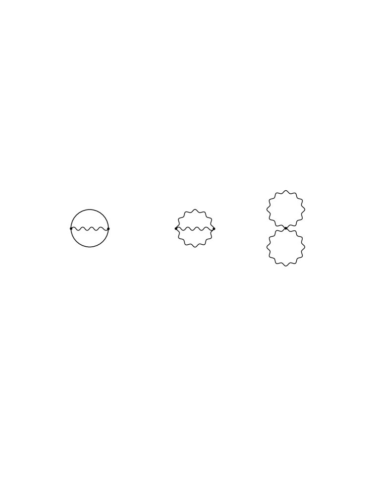
Figure 1: The two-loop approximation to $\Gamma_{2}$. Straight lines denote quark propagators, wavy lines denote gluon propagators.

The free energy is given by the CJT effective potential at its stationary points, determined by

$$\left.\frac{\delta\Gamma}{\delta\bar{\cal D}}\right|_{\bar{\cal D}={\cal D},\bar{\cal S}={\cal S}}=0\;,\;\;\;\;\left.\frac{\delta\Gamma}{\delta\bar{\cal S}}\right|_{\bar{\cal D}={\cal D},\bar{\cal S}={\cal S}}=0\;.$$ (7)

The first condition gives a Dyson-Schwinger equation for the gluon propagator,

$${\cal D}^{-1}=D^{-1}+\Pi[{\cal S}]\;.$$ (8)

One now sees that, at the stationary point, the second term in Eq. (4) cancels the last term,

$$\Gamma[{\cal D},{\cal S}]=\frac{T}{2\Omega}\left[{\rm Tr}\ln{\cal D}^{-1}-{\rm Tr}\ln{\cal S}^{-1}-{\rm Tr}(S^{-1}{\cal S}-1)\right]\;.$$ (9)

In terms of the gluon and quark propagators in the normal phase, ${\cal D}_{n}(K)$ and ${\cal S}_{n}(K)$, the propagators in the superconducting phase are written as

$${\cal S}(K) = {\cal S}_{n}(K)+\delta{\cal S}(K,\Delta)\;,$$ (10a)

$${\cal D}^{-1}(K) = {\cal D}_{n}^{-1}(K)+\delta\Pi(K,\Delta)\;,$$ (10b)

where $\delta\Pi\equiv\Pi-\Pi_{n}$, i.e., ${\cal D}_{n}^{-1}$ already contains the hard-dense-loop (HDL) resummed gluon self-energy $\Pi_{n}$. The gluon self-energy in the superconducting phase, $\Pi$, depends on the superconducting gap parameter, $\Delta$, and so $\delta\Pi$ also depends on $\Delta$. Similarly, the quark propagator in the normal phase ${\cal S}_{n}$ contains quark self-energy corrections, and $\delta{\cal S}$ depends on $\Delta$.

Inserting Eqs. (10) into Eq. (9), we obtain

$$\Gamma=\Gamma_{n}+{\Gamma}_{\rm cond}+{\Gamma}_{\rm fluc}+\Gamma_{\rm fluc}^{\prime}\;,$$ (11)

where

$$\Gamma_{n} = \frac{T}{2\,\Omega}\left[{\rm Tr}\ln{\cal D}_{n}^{-1}-{\rm Tr}\ln{\cal S}_{n}^{-1}-{\rm Tr}(S^{-1}{\cal S}_{n}-1)\right]\;,$$ (12a)

$${\Gamma_{\rm cond}} = \frac{T}{2\,\Omega}\left[{\rm Tr}({\cal D}_{n}{\delta}{\Pi})-{\rm Tr}(S^{-1}\delta{\cal S})+{\rm Tr}\ln(1+{\cal S}_{n}^{-1}\delta{\cal S})\right]\;,$$ (12b)

$${\Gamma}_{\rm fluc} = \frac{T}{2\,\Omega}{\sum_{\vec{k},\omega=0}}{\rm tr}\left\{\ln\left[1+{\cal D}_{n}(K){\delta}{\Pi}(K,\Delta)\right]-{\cal D}_{n}(K){\delta}{\Pi}(K,\Delta)\right\}\;,$$ (12c)

$${\Gamma}_{\rm fluc}^{\prime} = \frac{T}{2\,\Omega}{\sum_{\vec{k},\omega\neq 0}}{\rm tr}\left\{\ln\left[1+{\cal D}_{n}(K){\delta}{\Pi}(K,\Delta)\right]-{\cal D}_{n}(K){\delta}{\Pi}(K,\Delta)\right\}\;.$$ (12d)

The generalized GL free energy is the difference in the CJT effective potential between the superconducting phase and the normal phase, $\Gamma-\Gamma_{n}$. It includes both the ordinary GL terms and the fluctuation terms. Note that we have added a term ${\rm Tr}({\cal D}_{n}\delta\Pi)$ in $\Gamma_{\rm cond}$ and simultaneously subtracted it in $\Gamma_{\rm fluc},\Gamma_{\rm fluc}^{\prime}$. This term corresponds to the so-called exchange (free) energy kapusta and must be present in order to obtain the correct expression for $\Gamma_{\rm cond}$ Iida ; ioannis . Therefore, we have to subtract it in the fluctuation part of the free energy. Only with this subtraction, $\Gamma_{\rm fluc}+\Gamma_{\rm fluc}^{\prime}$ represents the well-known plasmon ring resummation kapusta . We note in passing that it is quite gratifying to see that the CJT formalism naturally contains all these different many-body contributions to the free energy.

In Ref. baym , the exchange energy was not subtracted from the plasmon ring contribution. This leads to an overall change of sign of the fluctuation energy. As shown below [see Eq. (19)], the contribution of the fluctuation energy is $\sim\ln(1+u)-u$, which is always negative, while in Ref. baym it is $\sim\ln(1+u)$ which is positive (for $u>0$). Therefore, the authors of Ref. baym concluded that gauge-field fluctuations raise the free energy of the color-superconducting phase, and thus decrease the transition temperature to the normal phase. In our case, however, the gauge-field fluctuations decrease the free energy, i.e., stabilize the color-superconducting phase and therefore lead to a larger transition temperature.

This is physically plausible if one remembers that gauge-field fluctuations are also present in the normal phase, namely in the first term in Eq. (12a). Since transverse gluons are massless in the normal phase, $\Pi_{n}(0)=0$, long-wavelength fluctuations are enhanced over those in the color-superconducting phase where gluons are massive, $\delta\Pi\neq 0$. Thus, the fluctuation energy in the normal phase is larger than in the superconducting phase.

As shown in the appendix, the weak-coupling approximation gives rise to Iida ; ioannis

$$\Gamma_{\rm cond}=\frac{6\mu^{2}}{\pi^{2}}\,t\,\Delta^{2}(T)+\frac{21\zeta(3)}{4\pi^{4}}\left(\frac{\mu}{T_{c}}\right)^{2}\Delta^{4}(T),$$ (13)

where $T_{c}$ is determined up to the accuracy of Eq. (1) and $t\equiv(T-T_{c})/T_{c}$ is the reduced temperature. The gap parameter of the fermionic quasiparticle excitations is $\Delta$ (8-fold) and $2\Delta$ (1-fold) rischke . One can check that the quadratic and quartic coefficients of $\Gamma_{\rm cond}$ for CSC are, respectively, 12 ($=8\times 1^{2}+2^{2}$) and 24 ($=8\times 1^{4}+2^{4}$) times larger than those for an electronic superconductor. The relevant fluctuation term is

$$\Gamma_{\rm fluc}=8\,T\int\frac{d^{3}\vec{k}}{(2\pi)^{3}}\left\{\ln\left[1+\frac{m^{2}(T,k)}{k^{2}}\right]-\frac{m^{2}(T,k)}{k^{2}}\right\},$$ (14)

while $\Gamma_{\rm fluc}^{\prime}$ is of higher order. The momentum-dependent Meissner mass reads

$$m^{2}(T,k)=\frac{1}{\lambda^{2}}f(k\xi_{0}),$$ (15)

with the chromomagnetic penetration depth given by

$$\frac{1}{\lambda^{2}}=\frac{7\zeta(3)}{24\pi^{4}}\frac{g^{2}\mu^{2}\Delta^{2}}{T_{c}^{2}},$$ (16)

and

$$f(y)=\frac{6}{7{\zeta}(3)}{\sum_{s=0}^{\infty}}{\int^{1}_{0}}dx\frac{1-x^{2}}{(s+{\frac{1}{2}})[4(s+{\frac{1}{2}})^{2}+y^{2}x^{2}]}\;.$$ (17)

Carrying out the integration in Eq. (14) and combining the result with Eq. (13), we find

$$\Gamma=\frac{6\mu^{2}}{\pi^{2}}\,t\,\Delta^{2}(T)+\frac{21\zeta(3)}{4\pi^{4}}\left(\frac{\mu}{T_{c}}\right)^{2}\Delta^{4}(T)+32\pi(T_{c})^{4}\,F\left(\frac{\xi_{0}^{2}}{\lambda^{2}(T)}\right),$$ (18)

where the function $F$ is defined by

$$F(z)={\int^{\infty}_{0}}dx\,x^{2}\left\{\ln\left[1+{\frac{z}{x^{2}}}f(x)\right]-\frac{z}{x^{2}}f(x)\right\}\;.$$ (19)

The London limit corresponds to small arguments in Eqs. (17) and (19). We have

$$f(y)=1-\frac{31}{140}\frac{\zeta(5)}{\zeta(3)}y^{2}+O(y^{4}),$$ (20)

and

$$F(z)\simeq-\frac{\pi}{3}z^{\frac{3}{2}}.$$ (21)

In the Pippard limit the arguments of $f(y)$ and $F(z)$ become large and we end up with

$$f(y)=\frac{3\pi^{3}}{28\zeta(3)y}\left[1-12\,\frac{4\ln y+4\ln 2+\gamma}{\pi^{3}y}+O(y^{-2})\right]$$ (22)

and

$$F(z)\simeq-\frac{3\pi^{3}}{28\zeta(3)}z\Big{[}\ln\Big{(}\frac{3\pi^{3}}{28\zeta(3)}z\Big{)}+{\rm const}\Big{]}.$$ (23)

Here we have retained the first corrections for both limits of the function $f(y)$ in order to assess the deviation from each limit at the CSC phase transition.

Before concluding this section, let us clarify once more several differences between our formulation and that of Ref. baym . First, since in their treatment the term $-m^{2}(T,k)/k^{2}$ in Eq. (14), which arises from the subtraction of the exchange energy, is missing, their formal power-series expansion for the fluctuation energy in terms of $\Delta$ starts already at quadratic order. This then gives rise to a renormalized critical temperature $T_{c}^{\prime}$. When including the term in question, there is no such renormalization of $T_{c}$. Nevertheless, the difference between $T_{c}$ and $T_{c}^{\prime}$ is of order $\mathcal{O}(g^{2})$, and the two-loop approximation employed in the derivation of Eq. (18) is not sufficiently accurate to provide all corrections of this order. Furthermore, the authors of Ref. baym approximated the momentum-dependent Meissner mass by a constant and simply cut off the momentum integration in Eq. (14). In that case, one is effectively in the London limit of Eqs. (17) and (19), where the fluctuation energy is of the form of Eq. (21). The shift in the transition temperature compared to that of Eq. (1) is then only of order $\mathcal{O}(g^{2})$ baym , and not of order $\mathcal{O}(g)$, as found here and in Ref. dirkfluct .

III The first-order CSC transition in weak coupling

A generic first-order phase transition can be described by three characteristic temperatures: the transition temperature $T_{c}^{*}$, the maximum temperature of the (metastable) superheated superphase $T_{\rm sh}$, and the minimum temperature of the (metastable) supercooled normal phase $T_{\rm sc}$, respectively. These temperatures are related in the following way,

$$T_{\rm sc}<T_{c}^{*}<T_{\rm sh}\;,$$ (24)

and they can be obtained from the generalized GL free energy (18). The lower margin of a supercooled normal phase corresponds to

$$\left.\frac{\partial^{2}\Gamma}{\partial\Delta^{2}}\right|_{\Delta=0}=0,$$ (25)

and, using Eq. (18), we have

$$T_{\rm sc}=T_{c}\;,$$ (26)

which relates $T_{\rm sc}$ with the onset temperature for diquark pairing. On the other hand, the transition occurs at

$$\frac{\partial\Gamma}{\partial\Delta}=0\;,\qquad\Gamma=0\;,$$ (27)

for a value of $\Delta\equiv\Delta_{c^{*}}\neq 0$. This implies that

$$t_{c}^{*} + \frac{7\zeta(3)}{4\pi^{2}}\frac{\Delta^{2}_{c^{*}}}{T^{2}_{c}}+\frac{7\zeta(3)}{18\pi^{3}}g^{2}F^{\prime}\left(\frac{\xi_{0}^{2}}{\lambda^{2}_{c^{*}}}\right)=0\;,$$

$$t_{c}^{*} + \frac{7\zeta(3)}{8\pi^{2}}\frac{\Delta^{2}_{c^{*}}}{T^{2}_{c}}+\frac{7\zeta(3)}{18\pi^{3}}g^{2}\frac{\lambda^{2}_{c^{*}}}{\xi_{0}^{2}}F\left(\frac{\xi_{0}^{2}}{\lambda^{2}_{c^{*}}}\right)=0\;.$$ (28)

Eliminating $t_{c}^{*}$ in the equations above we have

$${\cal F}\left(\frac{\xi_{0}^{2}}{\lambda^{2}_{c^{*}}}\right)=\frac{216{\pi}^{7}}{7{\zeta}(3)g^{4}}\left(\frac{T_{c}}{\mu}\right)^{2}\;,$$ (29)

where ${\cal F}(z)=-F^{\prime}(z)/z+F(z)/z^{2}$. Solving Eq. (29) for $\Delta^{2}_{c^{*}}$, with the aid of Eq. (23), we obtain

$$\Delta^{2}_{c^{*}}=\frac{\pi^{2}}{63{\zeta}(3)}\,g^{2}T^{2}_{c}\;.$$ (30)

The transition temperature is obtained substituting Eq. (30) into either one of Eqs. (28), which produces

$$T_{c}^{*}=\Big{(}1+\frac{\pi^{2}}{12\sqrt{2}}g\Big{)}\,T_{c}\;.$$ (31)

These were the results reported in Ref. dirkfluct . The penetration depth at the transition is

$$\frac{1}{\lambda^{2}_{c^{*}}}=\frac{g^{4}}{216\pi^{2}}\mu^{2}\;,$$ (32)

which yields the ratio

$$\frac{\xi_{0}^{2}}{\lambda^{2}_{c^{*}}}=\frac{g^{4}\mu^{2}}{864\pi^{4}T_{c}^{2}}\gg 1\;.$$ (33)

Thus, the Pippard limit is valid for the entire CSC phase at sufficiently large chemical potentials.

We shall proceed to determine $T_{\rm sh}$. The free energy $\Gamma$ as a function of $\Delta$ has a local maximum between $\Delta=0$ and the minimum $\Delta_{c^{*}}$ at $T=T_{c}^{*}$ in the superconducting phase. As $T$ increases, the local minimum remains unchanged until it coalesces with the local maximum, where

$$\frac{\partial\Gamma}{\partial\Delta}=0\;,\qquad\frac{\partial^{2}\Gamma}{\partial\Delta^{2}}=0\;,$$ (34)

for a value of $\Delta\equiv\Delta_{\rm sh}\neq 0$. It then follows that

$$t_{\rm sh}+\frac{7{\zeta}(3)}{4\pi^{2}}\frac{{\Delta^{2}_{\rm sh}}}{T^{2}_{c}} + \frac{7{\zeta}(3)}{18\pi^{3}}g^{2}F^{\prime}\left(\frac{\xi_{0}^{2}}{\lambda_{\rm sh}^{2}}\right)=0\;,$$

$$F^{\prime\prime}\left(\frac{\xi_{0}^{2}}{\lambda_{\rm sh}^{2}}\right) = -\frac{432\pi^{7}}{7\zeta(3)g^{4}}\Big{(}\frac{T_{c}}{\mu}\Big{)}^{2}\;.$$ (35)

Moreover, Eq. (35) together with Eq. (23) yields

$$\Delta^{2}_{\rm sh}=\frac{\pi^{2}}{126\zeta(3)}g^{2}T^{2}_{c^{*}}=\frac{1}{2}\Delta^{2}_{c^{*}}\;.$$ (36)

Subtracting the first equation in Eq. (28) from Eq. (35) and using (23), we find that

$$t_{\rm sh}-t_{c}^{*}=\frac{g^{2}}{72}(1-\ln{2})\;,$$ (37)

and as a result

$$T_{\rm sh}=\left[1+\frac{g^{2}}{72}(1-\ln{2})\right]T_{c}^{*}\;.$$ (38)

Note that $T_{c}^{*}$ is one order of $g$ closer to $T_{\rm sh}$ than to $T_{\rm sc}$. The ratio

$$\frac{\xi_{0}^{2}}{\lambda_{\rm sh}^{2}}=\frac{g^{4}\mu^{2}}{1728\pi^{4}T_{c}^{2}}$$ (39)

implies that even the metastable CSC state is in the Pippard limit in weak coupling. Although the diagrammatics behind the generalized GL free energy function (18) determine $T_{c}$ only up to subleading order, the leading-order differences among the three characteristic temperatures do not change if higher-order corrections to $T_{c}$ are included.

Another observable associated with the first-order phase transition is the latent heat $L=T_{c}{\Delta}S$, where $\Delta S$ is the change in entropy density at the transition. We have

$$\Delta S=-\Big{(}\frac{\partial\Gamma}{\partial T}\Big{)}_{\Delta=\Delta_{c}^{*}}=\frac{2g^{2}}{21\zeta(3)}{\mu^{2}}T_{c}\;,$$ (40)

and as a result

$$L=\frac{2g^{2}}{21\zeta(3)}{\mu^{2}}T^{2}_{c}\equiv\frac{6\mu^{2}}{\pi^{2}}\,\Delta_{c^{*}}^{2}\;.$$ (41)

Now we calculate the strength of the first-order phase transition as was defined in Ref. ma ,

$$t_{\rm HLM}=\frac{L}{{\Delta}c_{v}}\;,$$ (42)

where ${\Delta}c_{v}$ is the jump in specific heat at the second-order phase transition, ignoring the fluctuations. If we ignore the third term in Eq. (18) we recover the ordinary GL theory from which we find $\Delta c_{v}=24\mu^{2}T_{c}/[7\zeta(3)]$. Thus, we have

$$\frac{t_{\rm HLM}}{T_{c}}=\frac{g^{2}}{36}\;.$$ (43)

Note that Eq. (43) implies that the strength of the first-order phase transition weakens (logarithmically) with increasing chemical potential, which is in agreement with the fact that the second-order phase transition is recovered at asymptotically large densities. Note that for electronic superconductors, $t_{\rm HLM}/T_{c}\sim 10^{-6}$ ma which, for realistic values of $g\sim 1$ is much smaller than the right-hand side of Eq. (43).

IV Numerical results

Strictly speaking, the weak-coupling results in the previous section are only valid at ultra-high baryon densities such that $\mu\gg\Lambda_{\rm QCD}$. For quark matter that may exist inside a compact star $\mu$ is expected to be slightly higher than $\Lambda_{\rm QCD}$, and then the weak-coupling expansion becomes problematic. Nevertheless, we shall assume that the generalized GL free energy remains numerically reliable down to realistic quark densities. Even though this is not the case, the qualitative statement for the absence of the London limit in CSC may still survive, due to the reason given at the end of this section.

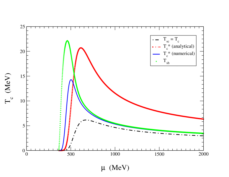
Figure 2: Comparison between the different temperatures involved in the discussion of the fluctuation-induced first-order phase transition.

We solved Eq. (29) and the second equation in Eq. (35) numerically in order to find $\Delta_{c^{*}}$ and $\Delta_{\rm sh}$ as functions of the chemical potential. The transition temperature $T_{c}^{*}$ is obtained using $\Delta_{c^{*}}$ in either one of Eqs. (28) and the temperature $T_{\rm sh}$ is obtained from the first equation in Eq. (35). We use the 3-loop formula for $\alpha_{s}=g^{2}/4\pi$ pdg ,

$$\alpha_{s}(\mu) = \frac{4\pi}{\beta_{0}\ln(\mu^{2}/\Lambda_{\rm QCD}^{2})}\left[1-\frac{2\beta_{1}}{\beta_{0}^{2}}\frac{\ln[\ln(\mu^{2}/\Lambda_{\rm QCD}^{2})]}{\ln(\mu^{2}/\Lambda_{\rm QCD}^{2})}\right.$$ (44)

$$+ \left.\frac{4\beta_{1}^{2}}{\beta_{0}^{4}[\ln(\mu^{2}/\Lambda_{\rm QCD}^{2})]^{2}}\left(\left\{\ln\left[\ln\left(\frac{\mu^{2}}{\Lambda_{\rm QCD}^{2}}\right)\right]-1/2\right\}^{2}+\frac{\beta_{2}\beta_{0}}{8\beta_{1}^{2}}-\frac{5}{4}\right)\right],$$

where $\beta_{0}=9$, $\beta_{1}=51-19/(3N_{f})=32$, $\beta_{2}=2857-5033N_{f}/9+325N_{f}^{2}/27$, for three colors and three flavors $N_{f}=3$. Moreover, we have taken $\Lambda_{QCD}=364$ MeV in our calculations, in order to obtain the correct value of $\alpha_{s}$ at the scale of the $Z$-boson mass.

Figure 2 shows the three temperatures $T_{\rm sc}$, $T_{c}^{*}$ and $T_{\rm sh}$ as functions of the chemical potential, along with the weak-coupling formula (31) obtained in Ref. dirkfluct . Note that $T_{c}^{*}$ is still closer to $T_{\rm sh}$ than to $T_{\rm sc}$ down to few hundreds of MeV.

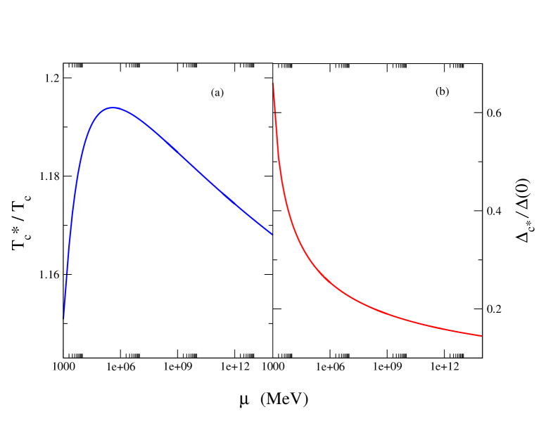
Figure 3: (a) Comparison between the critical temperatures at high densities. (b) Discontinuity of the gap at the transition.

A comparison between the numerically evaluated critical temperature $T_{c}^{*}$ and $T_{c}$ is shown in Fig. 3 (a) and the discontinuity of the gap at $T_{c}^{*}$, relative to its value at $T=0$, (2), is shown in Fig. 3 (b) shortpaper . Both plots indicate that

$$\lim_{\mu\to\infty}\frac{T_{c}^{*}}{T_{c}}=1\;,\qquad\lim_{\mu\to\infty}\frac{\Delta_{c^{*}}}{\Delta(0)}=0\;,$$ (45)

as expected, although the convergence is rather slow.

Now we will address the question of whether or not the London limit is realized near $T_{c}^{*}$ for color superconductors in the range of chemical potentials explored here. From Fig. 4 we see that the ratio $\xi_{0}/\lambda_{c^{*}}\gg 1$, meaning that only the Pippard limit of magnetic interactions is present in color superconductivity. Even for the minimum value of the ratio $\xi_{0}/\lambda_{c^{*}}$, which is around $\mu=700$ MeV, the Pippard expansion of $m^{2}(k,T)$ in Eq. (22) works better than the London expansion, displayed in Eq. (20). This is also the case for the metastable CSC state up to $T_{\rm sh}$, as is shown in Fig. 5.

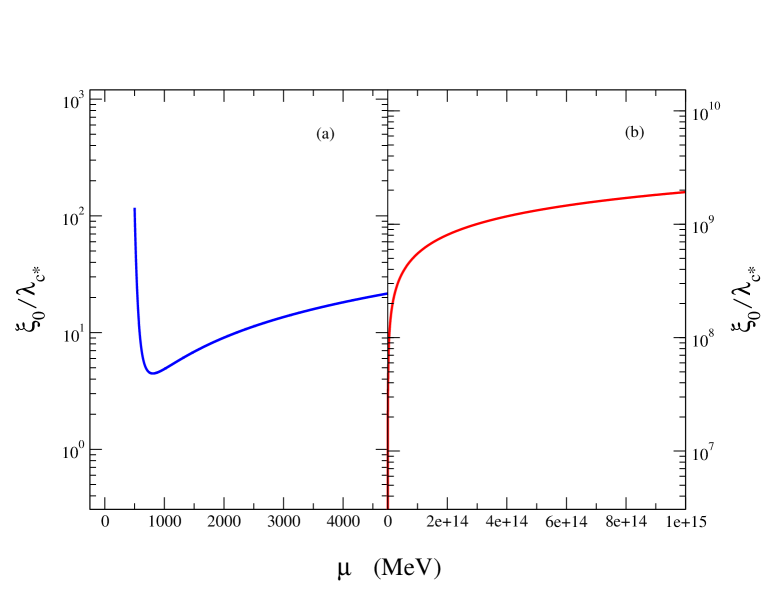
Figure 4: (a) $\xi_{0}/\lambda_{c^{*}}$ at small chemical potentials. (b) The same ratio at very large chemical potentials.

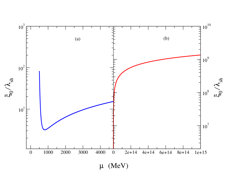
Figure 5: (a) $\xi_{0}/\lambda_{\rm sh}$ at small chemical potentials. (b) The same ratio at very large chemical potentials.

It is instructive to express the right-hand side of Eq. (29) in terms of the GL parameter (3) and compare it with the corresponding equation for a metallic superconductor, whose generalized GL free energy was given in Ref. dirkfluct . We have

$${\cal F}\Big{(}\frac{\xi_{0}^{2}}{\lambda^{2}_{c^{*}}}\Big{)}=\frac{3\pi^{2}\kappa^{2}}{16\alpha_{s}}\;,$$ (46)

for color superconductors and

$${\cal F}\Big{(}\frac{\xi_{0}^{2}}{\lambda^{2}_{c^{*}}}\Big{)}=\frac{\pi^{2}\kappa^{2}}{16\alpha_{e}v_{F}}\;,$$ (47)

for electronic superconductivity. A large value on the right-hand side of Eq. (46) or Eq. (47) points to the London limit at the first-order phase transition. Since $\alpha_{e}\ll\alpha_{s}$ and $v_{F}\sim\alpha_{e}$, the right-hand side of Eq. (47) is much larger than that of Eq. (46) under the same GL parameter. In other words, the London limit is more likely to be realized in metallic superconductors.

V Concluding remarks

In this paper we have systematically calculated the effects of gauge-field fluctuations on the free energy of a homogeneous CFL color superconductor in the Hartree-Fock approximation. We evaluated both analytically and numerically the temperature of the fluctuation-induced first-order phase transition, the latent heat, as well as the maximum temperature of a superheated superphase. It was also shown that the London limit for color-magnetic interactions in CFL color superconductors is absent. As the main reason we identified the weakness of electromagnetic interactions in comparison to strong interactions, $\alpha_{e}\ll\alpha_{s}$. Thus, one can say that once the gauge-field fluctuations are taken into account, the local-coupling approximation between the order parameter and the gauge fields is not valid in the CFL phase.

By using an inhomogeneous GL theory, Iida and Baym iidavortices investigated the formation of vortices and supercurrents induced by external magnetic fields and rotation in pairing states near the critical temperature. Since they used a mean-field approximation, all gauge fields were regarded as averaged quantities and fluctuations around their mean values were not considered. In order to see how the inclusion of fluctuations would change their results one has to derive an effective action that depends only on the order parameter and the gauge fields. This action would display non-local interactions between the gauge fields and the diquark condensate. Such an effective action could be obtained using the formalism developed in Ref. philipp .

It was shown in Ref. ma , by a one-loop renormalization-group calculation using the $\epsilon$ expansion, that no stable infrared fixed point can exist for a theory involving local interactions between abelian gauge fields and order parameters, unless the number of order parameter components, $N$, is artificially extended to $N>N_{c}=365$, which is far beyond the case of relevance for electronic superconductivity. This is then interpreted as signaling the presence of a first-order transition. Therefore, for electronic superconductors, gauge-field fluctuations are always expected to change the order of the phase transition to first order, irrespective of further details about the transition. For color superconductors the effective action containing only the order parameter and the gauge fields as well as the specific form of their interactions is not known, and the general result derived in Ref. ma may not be applicable. However, the results we obtained for the CFL phase seem to suggest that fluctuation-induced first-order phase transitions are indeed present in color superconductivity. Furthermore, due to the absence of the London limit, we expect that, once gauge-field fluctuations and first-order phase transitions are taken into account, local diquark-gluon interactions are never realized in color superconductors, regardless which phase is considered. This would constitute a striking new physical effect that would only come about in color superconductivity. In fact, the crossover from nonlocal to local interactions near the critical temperature in superconducting metals of strong type I has been recently observed bonalde . What we found in this paper rules out the possibility of observing such a crossover in color superconductors.

Recently, a GL free energy that takes into account the effects of nonzero quark masses and charge neutrality has been derived within the mean-field approximation Iidamass . A study on the validity of local diquark-gluon interactions in this case and the effects of gauge-field fluctuations on the phase diagram obtained in Ref. Iidamass is in progress and will be reported elsewhere future .

Appendix A

In this appendix, we sketch some important steps for the derivation of the generalized GL free energy in the presence of gauge-field fluctuations, which is shown in Eq. (18), in terms of Feynman diagrams. We have

$$\bigl{[}S^{-1}(P)\bigr{]}^{c_{1}c_{2}}_{f_{1}f_{2}} = (i\gamma_{\mu}P_{\mu}-\mu\gamma_{4}\rho_{3})\delta^{c_{1}c_{2}}\delta_{f_{1}f_{2}}\;,$$ (48a)

$$\bigl{[}\delta{\cal S}^{-1}(P)\bigr{]}^{c_{1}c_{2}}_{f_{1}f_{2}} = i\phi(P)\gamma_{5}\rho_{2}(\delta^{c_{1}}_{f_{1}}\delta^{c_{2}}_{f_{2}}-\delta^{c_{1}}_{f_{2}}\delta^{c_{2}}_{f_{1}})\;,$$ (48b)

$${\cal D}_{n}^{ll^{\prime}}(K)_{ij} \approx \frac{{\delta}^{ll^{\prime}}}{k^{2}+\frac{\pi}{4}m_{D}^{2}\frac{|\omega|}{k}}\left(\delta_{ij}-\frac{k_{i}k_{j}}{k^{2}}\right)\;,$$ (48c)

$${\cal D}_{n}^{ll^{\prime}}(K)_{j4} = 0\;,$$ (48d)

$${\cal D}_{n}^{ll^{\prime}}(K)_{44} \approx \frac{\delta^{ll^{\prime}}}{k^{2}+m_{D}^{2}},$$ (48e)

where $P=(\nu,\vec{p})$, $K=(\omega,\vec{k})$, $m_{D}^{2}=3\,g^{2}\mu^{2}/(2\pi^{2})$, $\rho$ represents Pauli matrices with respect to Nambu-Gorkov indices, $c_{i}$ and $l,l^{\prime}$ stand for the fundamental and adjoint color indices, respectively, $f_{i}$ are fundamental flavor indices, and $\nu$, $\mu$ correspond to discrete Matsubara frequencies. The symbol “$\approx$” in the gluon propagator means that we used the approximation for the total HDL gluon propagator that is relevant for the CSC energy scale.

Diagrammatically, ${\cal D}_{n}$ is denoted by a wavy line, ${\cal S}_{n}$ is represented by a thick line, and the CSC correction to the inverse quark propagator (A1b) is associated with a two-point vertex bearing a cross. The corresponding diagrammatic expansions for $\delta{\cal S}$ and $\delta\Pi$ are

In weak coupling we expand ${\cal S}_{n}$ as

Expanding $\,\Gamma_{\rm cond}$ up to the fourth power of $\phi(P)$ we find

where the weak-coupling approximation has been employed in order to retain the diagrams with at most one HDL gluon line. The diagram bearing two crosses yields the expression ${\sum_{PP^{\prime}}}\Phi(P)K(P|P^{\prime})\Phi(P^{\prime})$, where the kernel $K(P|P^{\prime})$ is isomorphic to the kernel in the Dyson-Schwinger equation for the diquark scattering amplitude in the normal phase. Moreover, taking $\Phi(P)$ to be proportional to the pairing mode, i.e.,

$$\phi(P)=\Delta\sin\Big{[}\,\frac{g}{3\sqrt{2}\pi}\ln\Big{(}\frac{1}{\hat{\nu}}\Big{)}\Big{]}\hskip 8.5359pt,$$ (49)

where $\Delta$ is the energy gap, $\hat{\nu}=(3/2)^{5/2}\,g^{5}\nu/(256\pi^{4}\mu)$, we have that

is proportional to $T-T_{c}$, with $T_{c}$ determined up to subleading order in $g$ [see Eq. (1)]. For the diagrams with four crosses the same mechanism yields

at $T=T_{c}$, which reduces the number of quartic terms in $\Gamma_{\rm cond}$. Moreover, it will be shown at the end of this appendix that the following two diagrams

(50)

are of higher order in weak coupling and can be dropped. For $\,\Gamma_{\rm cond}$ we end up with

which produces the terms in Eq. (13). Now we treat the fluctuation terms $\Gamma_{\rm fluc}+\Gamma^{\prime}_{\rm fluc}$ , whose diagrammatic representation is

  (51)

where $\Gamma_{\rm fluc}$ includes only the contribution from the static gluons and $\Gamma^{\prime}_{\rm fluc}$ contains remaining contributions. Due to the Meissner effect, the shaded bubble does not vanish when the spatial momentum of the gluon line goes to zero at zero Matsubara energy. A resummation of all ring diagrams in Eq. (51) is necessary for $\Gamma_{\rm fluc}$ and the result is the right-hand side of Eq. (14). Regarding $\Gamma^{\prime}_{\rm fluc}$, where the Matsubara energy of the gluon line is nonzero, dynamical screening prevents an infrared divergence for the integral over gluon momentum. In weak coupling $\Gamma^{\prime}_{\rm fluc}$ is dominated by the first diagram in Eq. (51), which is again of higher order. Therefore, the contribution of $\Gamma^{\prime}_{\rm fluc}$ can be safely neglected.

Now we present the argument supporting our assertion that the two diagrams in Eq. (50) and the first diagram in $\Gamma^{\prime}_{\rm fluc}$ can be neglected in weak coupling. Let us denote the contribution of the first diagram in Eq. (50) by $c_{1}\Delta^{4}$. It consists of five free quark propagators with four-momentum $(\nu,\vec{p})$ and a self-energy insertion $\Sigma(P)\sim g^{2}\nu\ln\left(\mu/|\nu|\right)\sim g\nu$. The main contribution to the $\vec{p}$-integration comes from a shell of thickness $\sim|\nu|$ around the Fermi surface and then we have

$$c_{1}\sim\mu^{2}T{\sum_{\nu}}\frac{1}{|\nu|^{4}}\,\Sigma(\nu)\sim g\,\frac{\mu^{2}}{T_{c}^{2}},$$ (52)

which is of ${\cal O}(g)$ in comparison to the quartic term in Eq. (13). The contribution of the second diagram in Eq. (50), denoted by $c_{2}\Delta^{4}$, can be estimated similarly. As is the case with the gap equation, the dominating contribution comes from the magnetic gluons with nonzero Matsubara energy. The integration for the quark propagators over the magnitude of their momenta $\vec{p}$, $\vec{p}$ ^′, on each side of the gluon line can be approximately decoupled from the integration for the gluon propagator over the angle between $\vec{p}$ and $\vec{p}$ ^′, where the latter produces the forward logarithm. We then find

$$c_{2}\sim g^{2}T^{2}\mu^{4}{\sum_{\nu\not=\nu^{\prime}}}\frac{1}{\nu^{2}\nu^{\prime 2}}\,\frac{1}{\mu^{2}}\ln\left(\frac{\mu}{\nu-\nu^{\prime}}\right)\sim g\,\frac{\mu^{2}}{T_{c}^{2}},$$ (53)

which is again of higher order. Now we consider the first diagram in $\Gamma^{\prime}_{\rm fluc}$ and denote its contribution as $c_{3}\Delta^{4}$. Since the typical momentum for the gluon line is $k\sim m_{D}^{2/3}|\omega|^{1/3}\gg\omega$ and $\omega\sim T_{c}$, each bubble can be approximated by the static magnetic self-energy of gluons at the Pippard limit, i.e.,

$$c_{3}\sim g^{4}T{\sum_{\omega\not=0}}\int\frac{d^{3}\vec{k}}{(2\pi)^{3}}\,\frac{1}{(k^{2}+\frac{\pi}{4}m_{D}^{2}\frac{|\omega|}{k})^{2}}\left(\frac{\mu^{2}}{T_{c}^{2}}\,\frac{T_{c}}{k}\right)^{2}\sim\frac{g^{4}\mu^{4}}{T_{c}^{2}m_{D}^{2}}{\sum_{\omega\not=0}}\frac{1}{|\omega|}\,.$$ (54)

The sum over $\omega$ has a cutoff when $\omega\sim m_{D}$ and then we end up with ${\sum_{\omega\not=0}}|\omega|^{-1}\sim\ln\left(\mu/T_{c}\right)\sim 1/g$. Consequently, we have $c_{3}\sim g\,\mu^{2}/T_{c}^{2}$, which is also negligible.

References

- (1) D. Ivanenko and D.F. Kurdgelaidze, Astrofiz. 1, 479 (1965); Lett. Nuovo Cim. 2, 13 (1969); N. Itoh, Prog. Theor. Phys. 44, 291 (1970); F. Iachello, W.D. Langer, and A. Lande, Nucl. Phys. A 219, 612 (1974).
- (2) H.D. Politzer, Phys. Rev. Lett. 30, 1346 (1973); D.J. Gross and F. Wilczek, Phys. Rev. D 8, 3633 (1973); Phys. Rev. D 9, 980 (1974).
- (3) J.C. Collins and M.J. Perry, Phys. Rev. Lett. 34, 1353 (1975).
- (4) For early works, see: D. Bailin and A. Love, Phys. Rept. 107, 325 (1984), and references therein.
- (5) M. Alford, K. Rajagopal, and F. Wilczek, Nucl. Phys. B 537, 443 (1999); R. Rapp, T. Schäfer, E.V. Shuryak, and M. Velkovsky, Phys. Rev. Lett. 81, 53 (1998); K. Rajagopal and F. Wilczek, hep-ph/0011333, to appear as Chapter 35 in the Festschrift in honor of B.L. Ioffe, At the Frontier of Particle Physics/Handbook of QCD, M. Shifman ed., (World Scientific 2001); M. Alford, Ann. Rev. Nucl. Part. Sci. 51, 131 (2001); T. Schäfer, hep-ph/0304281; H.-c. Ren, hep-ph/0404074, and references therein.
- (6) D.H. Rischke, Prog. Part. Nucl. Phys. 52, 197 (2004).
- (7) I.A. Shovkovy, Found. Phys. 35, 1309 (2005); M. Huang, Int. J. Mod. Phys. E 14, 675 (2005); T. Schäfer, hep-ph/0509068.
- (8) T. Schäfer and K. Schwenzer, Phys. Rev. D 70, 114037 (2004); H. Grigorian, D. Blaschke, and D. Voskresensky, Phys. Rev. C 71, 045801 (2005); D.N. Aguilera, D. Blaschke, M. Buballa, and V.L. Yudichev, Phys. Rev. D 72, 034008 (2005); P. Jaikumar, C.D. Roberts, and A. Sedrakian, nucl-th/0509093; A. Schmitt, I.A. Shovkovy, and Q. Wang, Phys. Rev. D 73, 034012 (2006).
- (9) J. Madsen, Phys. Rev. Lett. 85, 10 (2000); C. Manuel, A. Dobado, and F.J. Llanes-Estrada, JHEP 0509, 076 (2005).
- (10) D.T. Son, Phys. Rev. D 59, 094019 (1999).
- (11) T. Schäfer and F. Wilczek, Phys. Rev. D 60, 114033 (1999); R.D. Pisarski and D.H. Rischke, Phys. Rev. D 61 051501 (2000); D.K. Hong, V.A. Miransky, I.A. Shovkovy, and L.C.R. Wijewardhana, Phys. Rev. D 61 056001 (2000), [Erratum-ibid. D 62, 059903 (2000)]; W.E. Brown, J.T. Liu, and H.-c. Ren, Phys. Rev. D 61, 114012 (2000), Phys. Rev. D 62, 054016, 054013, (2000); Q. Wang and D.H. Rischke, Phys. Rev. D 65, 054005 (2002).
- (12) I. Giannakis and H.-c. Ren, Nucl. Phys. B 669, 462 (2003).
- (13) B.I. Halperin, T.C. Lubensky, and S. Ma, Phys. Rev. Lett. 32, 292 (1974).
- (14) See, for instance, E.M. Lifshitz and L.P. Pitaevskii, Statistical Physics (Pergamon Press, New York, 1980); see also V.P. Gusynin and I.A. Shovkovy, Nucl. Phys. A 700, 577 (2002) for the case of a color superconductor.
- (15) I. Bonalde, B.D. Yanoff, M.B. Salamon, and E.E.M. Chia, Phys. Rev. B 67, 012506 (2003).
- (16) I. Giannakis, D. Hou, H.-c. Ren, and D.H. Rischke, Phys. Rev. Lett. 93, 232301 (2004).
- (17) A.L. Fetter and J.D. Walecka, Quantum Theory of Many-Particle Systems (McGraw Hill, New York, 1971); J.I. Kapusta, Finite-temperature field theory (Cambridge University Press, Cambridge, 1989).
- (18) K. Iida and G. Baym, Phys. Rev. D 63, 074018 (2001).
- (19) I. Giannakis and H.-c. Ren, Phys. Rev. D 65, 054017 (2002).
- (20) T. Matsuura, K. Iida, T. Hatsuda, and G. Baym, Phys. Rev. D 69, 074012 (2004).
- (21) D.H. Rischke, Phys. Rev. D 62, 054017 (2000).
- (22) Review of Particle Physics by Particle Data Group, Phys. Rev. D 66, 010001 (2002).
- (23) J.L. Noronha, I. Giannakis, D. Hou, H.-c. Ren, and D.H. Rischke, nucl-th/0511047, to appear in the proceedings of 18th International Conference on Ultrarelativistic Nucleus-Nucleus Collisions: Quark Matter 2005 (QM 2005), Budapest, Hungary, 4-9 Aug 2005.
- (24) K. Iida and G. Baym, Phys. Rev. D 66, 014015 (2002), [Erratum-ibid., Phys. Rev. D 66, 059903(E) (2002)].
- (25) P.T. Reuter, Q. Wang, and D.H. Rischke, Phys. Rev. D 70, 114029 (2004); Erratum-ibid. D 71, 099901 (2005).
- (26) K. Iida, T. Matsuura, M. Tachibana, and T. Hatsuda, Phys. Rev. D 71, 054003 (2005).
- (27) J.L. Noronha, I. Giannakis, D. Hou, H.-c. Ren, and D.H. Rischke, in preparation.