Dynamical mass generation in strongly coupled Quantum Electrodynamics with weak magnetic fields

Abstract

We study the dynamical generation of masses for fundamental fermions in quenched quantum electrodynamics in the presence of weak magnetic fields using Schwinger-Dyson equations. Contrary to the case where the magnetic field is strong, in the weak field limit the coupling should exceed certain critical value in order for the generation of masses to take place, just as in the case where no magnetic field is present. The weak field limit is defined as $eB\ll m(0)^{2}$, where $m(0)$ is the value of the dynamically generated mass in the absence of the field. We carry out a numerical analysis to study the magnetic field dependence of the mass function above critical coupling and show that in this regime the dynamically generated mass and the chiral condensate for the lowest Landau level increase proportionally to $(eB)^{2}$.

It is well known that in QED, fermions can acquire masses through self interactions without the need of a nonzero bare mass. This phenomenon, known as dynamical mass generation (DMG), happens above a certain critical value of the coupling and its description can only be carried out in terms of non-perturbative treatments. Schwinger-Dyson Equations (SDEs) provide a natural platform to study DMG. In the quenched version of QED, a favorite starting point is to make an ansatz for the fermion-photon vertex and then study the fermion propagator equation in its decoupled form. It is also well known that in the presence of strong magnetic fields, it is possible to generate fermion masses for any value of the coupling. This phenomenon has been given the name of magnetic catalysis Gusynin ; Leung ; Hong ; Ferrer . Non-perturbative aspects of dynamical mass generation in the presence of weak magnetic fields have earlier been considered in the context of Nambu–Jona-Lasinio (NJL) model GusNJL , QCD Shushpanov and (2+1)-dimensional QED Farakos . In the context of QED4, the only work to our knowledge, is that of Kikuchi and Ng Kikuchi . However, they concentrate mainly on the behaviour of the critical coupling in the presence of the weak magnetic fields. In this paper, we undertake the study of the weak field dependence of the dynamically generated mass and the chiral condensate in QED in the rainbow truncation of SDE.

The SDE for the fermion propagator without external fields (in vacuum) in the rainbow approximation is

$$S_{F}^{-1}(p)=S_{F}^{(0)\,-1}(p)-\frac{i\alpha}{4\pi^{3}}\int d^{4}k\ \gamma^{\mu}S_{F}(k)\gamma^{\nu}\Delta_{\mu\nu}^{(0)}(q),$$ (1)

where $q\!=\!k\!-\!p$ and $\alpha=e^{2}/(4\pi)$ is the electromagnetic coupling constant. In this expression $\Delta_{\mu\nu}^{(0)}(q)$ is the bare photon propagator, which in covariant gauges is written as $\Delta_{\mu\nu}^{(0)}(q)=-\left(g_{\mu\nu}+(\xi-1)q_{\mu}q_{\nu}/q^{2}\right)/q^{2}$, $\xi$ being the usual covariant gauge parameter. We write the full fermion propagator as $S_{F}(p)={F(p^{2})}/{({\not\!p}-M(p^{2}))}$. $F(p^{2})$ is referred to as the wave function renormalization and $M(p^{2})$ as the mass function. In the Landau gauge $(\xi=0)$ $F(p^{2})=1$ and the mass function has nontrivial solutions for values of the coupling above the critical value $\alpha_{c}=\pi/3$. In the presence of external fields, SDEs have been a subject of study already for some time, see for example Ref. gitman .

When the magnetic field is strong, Landau levels are separated from each other by an amount $\sim\sqrt{eB}$ in such a way that for any value of the coupling $\alpha$, only the lowest Landau level (LLL) contributes to the DMG Gusynin ; Leung ; Hong ; Ferrer . However, in the case of weak external magnetic fields, Landau levels are close to each other and hence all contributions should be taken into account, which adds considerably to the complexity of the problem, as emphasized also in the fourth article of reference Gusynin .

The presence of the field breaks Lorentz invariance. Consequently, a simple Fourier transform on a single momentum variable is not possible. Nevertheless, it has been shown Ritus that the mass operator in the presence of an electromagnetic field can be written as a combination of the structures

$$\gamma^{\mu}\Pi_{\mu}\,,\,\sigma^{\mu\nu}F_{\mu\nu}\,,\,(F_{\mu\nu}\Pi^{\nu})^{2}\,,\,\gamma_{5}F_{\mu\nu}\tilde{F}^{\mu\nu}$$ (2)

which commute with the operator $(\gamma\cdot\Pi)^{2}$, where $\Pi_{\mu}\!=\!i\partial_{\mu}\!-\!eA^{\mbox{\tiny{ext}}}_{\mu},\ F_{\mu\nu}\!=\!\partial_{\mu}A^{\mbox{\tiny{ext}}}_{\nu}\!-\!\partial_{\nu}A^{\mbox{\tiny{ext}}}_{\mu},\ \tilde{F}^{\mu\nu}=\frac{1}{2}\epsilon^{\mu\nu\lambda\tau}F_{\lambda\tau},\ \sigma_{\mu\nu}=i[\gamma_{\mu},\gamma_{\nu}]/2$ and $A^{\mbox{\tiny{ext}}}$ is the external vector potential. We take $A^{\mbox{\tiny{ext}}}_{\mu}=B(0,-y/2,x/2,0)$ which describes a constant magnetic field ${\mathbf{B}}=B{\mathbf{\hat{z}}}$ vanish .

In order to find a diagonal representation for the mass operator, we thus need to find the eigenfunctions $\psi_{p\sigma}$ of the operator $(\gamma\cdot\Pi)^{2}$, namely

$$(\gamma\cdot\Pi)^{2}\psi_{p\sigma}u_{\sigma\chi}=p^{2}\psi_{p\sigma}u_{\sigma\chi}\,,$$ (3)

where $u_{\sigma\chi}$ are taken as the eigenspinors of $\Sigma_{3}$ and $\gamma_{5}$. We work in cylindrical coordinates ${\bf r}=(r,\phi,z)$ and in the chiral representation of the $\gamma-$matrices where $\Sigma_{3}$ and $\gamma_{5}$ are both diagonal with eigenvalues $\sigma=\pm 1$ and $\chi=\pm 1$. The normalized eigenfunctions $\psi_{p\sigma}$ (see for example Ref. Sokolov ) are given by

$$\psi_{p\sigma}(t,{\bf r})=Ne^{-i(E_{p}t-p_{z}z)}e^{i(l_{p}-\frac{(\sigma+1)}{2})\phi}I_{n_{p}-\frac{(\sigma+1)}{2}}^{s_{p}}(\rho)$$ (4)

where $N=\sqrt{2\gamma/(2\pi)^{3}}$, $\rho=\gamma r^{2}$, $\gamma=eB/2$, $p^{2}=E_{p}^{2}-p_{z}^{2}-2eBn$ and

$$I_{n}^{s}(\rho)=\sqrt{\frac{s!}{n!}}e^{-\rho/2}\rho^{(n-s)/2}L_{s}^{n-s}(\rho)$$ (5)

are the Laguerre functions footnote1 with the quantum numbers $n,l,s$ related by $n=l+s$. Since the problem involves only a magnetic field, the solutions do not depend on the eigenvalues $\chi$.

The solutions can be conveniently arranged in a matrix form

$$\Psi_{p}(x)=\sum_{\sigma=\pm 1}\psi_{p\sigma}(x)\Delta(\sigma)$$ (6)

where $\Delta(\sigma)\equiv{\mbox{diag}}\left\{\delta_{\sigma 1},\delta_{\sigma-1},\delta_{\sigma 1},\delta_{\sigma-1}\right\}$ is a $4\times 4$ matrix and $x=(t,{\bf r})$.

The matrix in Eq. (6) is used to rotate the two-point fermion Green’s function between coordinate, $G(x,y)$ and momentum spaces, ${\mathcal{G}}(k)$, as

$$G(x,y)=\sum_{n_{k},s_{k}}\int d^{2}k_{\parallel}\Psi_{k}(x){\mathcal{G}}(k)\bar{\Psi}_{k}(y)\,,$$ (7)

where $k_{\parallel}=(k_{0},0,0,k_{3})$ and $\bar{\Psi}_{k}=\gamma^{0}\Psi^{\dagger}_{k}\gamma^{0}$. The above expression can be substituted into the equation relating the two-point fermion Green’s function and the mass operator $M(x,y)$ in coordinate space, namely

$$\gamma\cdot\Pi(x)G(x,y)\!-\!\!\int\!\!d^{4}x^{\prime}M(x,x^{\prime})G(x^{\prime},y)=\delta^{4}(x-y)$$ (8)

to find the explicit form for the function ${\mathcal{G}}$ in momentum space, which is given by

$${\mathcal{G}}(k)=\frac{1}{\gamma\cdot k-\Sigma(k)}\,.$$ (9)

In order to arrive at this equation, we have used the completeness of the functions $\psi_{k\sigma}$ expressed in terms of $\Psi_{k}$ as

$$\sum_{n_{k},s_{k}}\int d^{2}k_{\parallel}\Psi_{k}(x)\bar{\Psi}_{k}(y)=\delta^{4}(x-y)$$ (10)

along with the properties

$$\gamma\cdot\Pi(x)\Psi_{k}(x) = \Psi_{k}(x)(\gamma\cdot k)$$

$$\int d^{4}x^{\prime}M(x,x^{\prime})\Psi_{k}(x^{\prime}) = \Psi_{k}(x)\Sigma(k)\,,$$ (11)

and the definition of the mass operator $\Sigma(k)$ in momentum space

$$M(k,k^{\prime}) \equiv \int d^{4}xd^{4}x^{\prime}\bar{\Psi}_{k}(x)M(x,x^{\prime})\Psi_{k^{\prime}}(x^{\prime})$$ (12)

$$= \delta_{n_{k}n_{k^{\prime}}}\delta_{s_{k}s_{k^{\prime}}}\delta^{2}(k_{\parallel}-k^{\prime}_{\parallel})\Sigma(k)\,.$$

With the aid of Eqs. (9)–(12) it is now straightforward to transform the SDE for the mass operator in the rainbow approximation from coordinate space, namely,

$$M(x,x^{\prime})=-ie^{2}\gamma^{\mu}G(x,x^{\prime})\gamma^{\nu}D^{(0)}_{\mu\nu}(x-x^{\prime})\,,$$ (13)

to momentum space, which now reads

$$\delta_{n_{p}n_{p^{\prime}}}\delta_{s_{p}s_{p^{\prime}}}\delta^{2}(p_{\parallel}-p^{\prime}_{\parallel})\Sigma(p)=-ie^{2}\int d^{4}xd^{4}x^{\prime}\sum_{n_{k},s_{k}}\int d^{2}k_{\parallel}\bar{\Psi}_{p}(x)\gamma^{\mu}\Psi_{k}(x)\frac{D^{(0)}_{\mu\nu}(x-x^{\prime})}{\gamma\cdot k-\Sigma(k)}\bar{\Psi}_{k}(x^{\prime})\gamma^{\nu}\Psi_{p^{\prime}}(x^{\prime})\,,$$ (14)

where the bare photon propagator is

$$D^{(0)}_{\mu\nu}(x-x^{\prime})=\int\frac{d^{4}q}{(2\pi)^{4}}\frac{e^{-iq\cdot(x-x^{\prime})}}{q^{2}+i\epsilon}\Delta^{(0)}_{\mu\nu}(q)\,.$$ (15)

Having considered the dependence of the mass function $\Sigma(k)$ on the structures in Eq. (2), its remaining, most general form can be written as ${\not\!k}-\Sigma(k)={\mathcal{F}}^{-1}(k)\left[{\not\!k}-{\mathcal{M}}(k)\right]\,,$ where, as in the case of vacuum, ${\mathcal{F}}(k)$ and ${\mathcal{M}}(k)$ are called the wave function renormalization and mass functions, respectively, in the presence of the field. We work in the Landau gauge ($\xi=0$) where we know that for vacuum $F=1$. Since we aim at a description for small magnetic field strengths, we naturally expect ${\mathcal{F}}\sim 1$ in the Landau gauge. Furthermore, let us work with the ansatz that ${\mathcal{M}}(k)$ is proportional to the unit matrix. Weakness of the magnetic field also implies that the bare vertex is a reasonable choice in the sense that Ward Identity is satisfied in the Landau gauge up to a correction connected with the mass function ${\mathcal{M}}(k)$. This correction might be expected to be small because ${\mathcal{M}}(k)\sim{\mathcal{M}}(p)$ for small values of momenta as the mass function is practically a constant, and it falls off sharply as $1/k$ for large momenta.

The self-consistent equation for the mass function is obtained by considering the diagonal part $(n_{p}=n_{p^{\prime}}\ s_{p}=s_{p^{\prime}})$ and taking the trace of Eq. (14). The integrals over $x$ and $x^{\prime}$ in Eq. (14) are readily performed. Having set $n_{p}=n_{p^{\prime}}\ s_{p}=s_{p^{\prime}}$, the integral over $x$ is just the complex conjugate of the one over $x^{\prime}$. The first one is found from the expression

$$\int d^{4}x\psi^{*}_{p\sigma_{p}}(x)\psi_{k\sigma_{k}}(x)e^{-iq\cdot x} = \delta^{2}(p_{\parallel}-k_{\parallel}-q_{\parallel})(-1)^{s_{k}-(\sigma_{p}+1)/2}\sqrt{\frac{(n_{p}-(\sigma_{p}+1)/2)!s_{k}!}{(n_{k}-(\sigma_{k}+1)/2)!s_{p}!}}$$ (16)

$$\times\left(\frac{q_{\perp}^{2}}{4\gamma}\right)^{(l_{k}-l_{p})/2-(\sigma_{k}-\sigma_{p})/4}e^{-q_{\perp}^{2}/4\gamma}L_{n_{p}-(\sigma_{p}+1)/2}^{n_{k}-n_{p}-(\sigma_{k}-\sigma_{p})/2}(q_{\perp}^{2}/4\gamma)L_{s_{k}}^{s_{p}-s_{k}}(q_{\perp}^{2}/4\gamma)\,,$$

where $q_{\perp}=(0,q_{1},q_{2},0)$. Equation (16) is real and thus, integrating over $x$ and $x^{\prime}$ in Eq. (14), results in the square of the right-hand side of Eq. (16). The presence of the delta function in this last equation, allows easy integration over $k_{\parallel}$. Gathering the above described elements, we obtain self-consistent equation for the mass function

$${\mathcal{M}}(p_{\parallel},n_{p}) = \frac{-ie^{2}}{2}\sum_{\sigma_{k},\sigma_{p}=\pm 1}\sum_{n_{k},s_{k}}\frac{s_{p}!s_{k}!}{(n_{p}-\frac{(\sigma_{p}+1)}{2})!(n_{k}-\frac{(\sigma_{k}+1)}{2})!}\int\frac{d^{4}q}{(2\pi)^{4}}\frac{e^{-q_{\perp}^{2}/2\gamma}}{q^{2}+i\epsilon}\frac{{\mathcal{M}}((p-q)_{\parallel},n_{k})}{(p-q)_{\parallel}^{2}-2eBn_{k}-{\mathcal{M}}^{2}((p-q)_{\parallel},n_{k})}$$ (17)

$$\left(\frac{q_{\perp}^{2}}{4\gamma}\right)^{l_{k}-l_{p}-\frac{(\sigma_{k}-\sigma_{p})}{2}}\!\!\left[2+\frac{1}{q^{2}}\left(q_{\perp}^{2}(1-\delta_{\sigma_{p}\sigma_{k}})-q_{\parallel}^{2}\delta_{\sigma_{p}\sigma_{k}}\right)\right]\!\!\left[L_{n_{p}-\frac{(\sigma_{p}+1)}{2}}^{n_{k}-n_{p}-\frac{(\sigma_{k}-\sigma_{p})}{2}}(q_{\perp}^{2}/4\gamma)\right]^{2}\!\!\!\!\left[L_{s_{k}}^{s_{p}-s_{k}}(q_{\perp}^{2}/4\gamma)\right]^{2}\,,$$

where in the notation for the mass function we have emphasized the breakdown of Lorentz invariance. We expect that ${\mathcal{M}}((p-q)_{\parallel},n_{k})$ should be independent of $s_{k}$ since the energy only depends on the principal quantum number $n_{k}$. Furthermore we assume that ${\mathcal{M}}((p-q)_{\parallel},n_{k})$ is a slowly varying function of $n_{k}$ and thus make the approximation ${\mathcal{M}}((p-q)_{\parallel},n_{k})\sim{\mathcal{M}}((p-q)_{\parallel},n_{k}=0)$. For consistency we consider the case $n_{p}=0$. Hereafter, we employ the more convenient notation ${\mathcal{M}}(k_{\parallel},n_{k}=0)\equiv{\mathcal{M}}(k_{\parallel})$ for generic arguments of the mass function. With these considerations the sum over $s_{k}$ can be computed by means of the result in Ref. Gautam . It is worth mentioning that after summing over $s_{k}$, the resulting equation is the same as Eq. (50) in Ref. Leung when considering the case $n_{k}=0$, which corresponds to the strong field limit.

In the situation where the magnetic field is weak, we expand $[(p-q)_{\parallel}^{2}-2eBn_{k}-{\mathcal{M}}^{2}((p-q)_{\parallel})]^{-1}$ as a geometric series in powers of $eB$. The remaining sum over $n_{k}$ can be performed also by resorting to Ref. Gautam yielding, after a Wick rotation

$${\mathcal{M}}(p_{\parallel}) \simeq \frac{\alpha}{4\pi^{3}}\int d^{4}q\frac{{\mathcal{M}}((p-q)_{\parallel})}{q^{2}[(p-q)_{\parallel}^{2}+q_{\perp}^{2}+{\mathcal{M}}^{2}((p-q)_{\parallel})]}\left\{3+\left[\frac{4}{[(p-q)_{\parallel}^{2}+q_{\perp}^{2}+{\mathcal{M}}^{2}((p-q)_{\parallel})]^{2}}\right.\right.$$ (18)

$$- \left.\left.\frac{6(6-q_{\perp}^{2}/q^{2})q_{\perp}^{2}}{[(p-q)_{\parallel}^{2}+q_{\perp}^{2}+{\mathcal{M}}^{2}((p-q)_{\parallel})]^{3}}+\frac{36q_{\perp}^{4}}{[(p-q)_{\parallel}^{2}+q_{\perp}^{2}+{\mathcal{M}}^{2}((p-q)_{\parallel})]^{4}}\right](eB)^{2}\right\}\,,$$

keeping only the lowest order contribution in $eB$. Notice that, as expected, the $s_{p}$ dependence of the mass function disappears on carrying out the sum over $s_{k}$.

Solving the above equation numerically is still not trivial, owing to the fact that the unknown function ${\mathcal{M}}((p-q)_{\parallel})$ within the integral is Lorentz non-invariant. However, we can always expand it out in powers of $(eB)^{2}$. Therefore, ${\mathcal{M}}((p-q)_{\parallel})={\mathcal{M}}_{0}(p-q)+(eB)^{2}{\mathcal{M}_{1}}$, where ${\mathcal{M}_{1}}$ is responsible for breaking the Lorentz invariance of ${\mathcal{M}}_{0}(p-q)$.

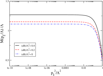
Figure 1: Mass function in the LLL for different values of the weak external magnetic field for $\alpha=6.5\alpha_{c}$.

Consistently, we carry out the same expansion on the left hand side of Eq. (18). As the Lorentz invariance should be restored for the leading terms, we justifiably complete the momenta to achieve the same. This filters out the vacuum result. To calculate the magnetic field effect, we solve the integral equation for ${\mathcal{M}_{1}}$ obtained by comparing powers of $(eB)^{2}$. The results for ${\mathcal{M}}(p_{\parallel}/\Lambda)$ in the LLL are depicted in Fig. 1, scaled by the ultraviolet cut-off $\Lambda$. Note that the results have been shown for a value of the coupling significantly above the critical value only for the magnetic field dependence to stand out. The same qualitative behaviour persists even in the immediate vicinity of the critical coupling, footnote2 .

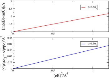
Figure 2: Magnetic contribution to the dynamically generated mass (upper graph) and condensate (lower graph) in the LLL as a function of $(eB)^{2}$ for $\alpha=6.5\alpha_{c}$.

The dot-dashed line corresponds to the vacuum. The effect of the external field is to increase the dynamically generated mass, preserving the qualitative features of the mass function profile. We have numerically verified that the critical value of the coupling is independent of the strength of the magnetic field, which is consistent with the findings of Ref. Kikuchi . To see the magnetic contribution to the dynamically generated mass, we show in Fig. 2 the difference $m(eB)-m(0)$, as a function of $(eB)^{2}$, where $m$ is the dynamical fermion mass, namely, $m\equiv{\mathcal{M}}(0)$. Notice that this difference grows linearly with $(eB)^{2}$. This is the same behaviour as was observed for the NJL model in GusNJL . We also evaluate the condensate defined as $\langle\bar{\psi}\psi\rangle=i\ {\rm Tr}\ G(x,x)$. In the weak field limit, spacing between Landau levels becomes small. To compute the condensate, the sum over these levels, can be carried out by replacing $\sum_{n}$ with the integral $\int d^{2}k_{\perp}/(2\pi\ eB)$, along with the substitution $2eBn\rightarrow k_{\perp}^{2}$. The weak field contribution to the condensate also turns out to be quadratic and with the above mentioned substitutions, it owes itself entirely to the non Lorentz invariant piece of the mass function in our computational set up. Its behavior as a function of $(eB)^{2}$ is also shown in Fig. 2.

In summary, we have shown that for $\alpha>\alpha_{c}$ the dynamically generated mass increases quadratically with the magnetic field strength. As compared to the strong field case, this is a four-fold dependence on the magnetic field Gusynin ; Hong ; Leung ; Ferrer . Such a dependence is similar to that found in GusNJL for the NJL model. In the supercritical phase of QED, i.e, $\alpha>\alpha_{c}$, the gap equation of Ref. Kikuchi can be solved in the linearized approximation, giving the same quadratic dependence as we have demonstrated through explicit numerical evaluation of the SDE in our setup private . It is ineteresting to note that Farakos et. al. Farakos also report similar behaviour in (2+1)-dimensional QED. Authors of this work employ the Schwinger proper time method, neglecting the field dependent phase of the fermion propagator. Therefore, a direct comparison with our findings is not straightforward. Contrary to the widely studied case when the field is strong and the LLL dominates, all the Landau levels should be taken into account in the weak field limit. This feature makes the problem a difficult one and hence has been discussed less frequently in literature. Here we have shown that under plausible assumptions about the behavior of the mass function, the sum over Landau levels can be performed. The relaxation of some of the assumptions made is a natural generalization of this work, along with the inclusion of a thermal bath and the study of the gauge dependence of the results in the context of the Ward identities Ferrer2 and the Landau-Khalatnikov-Fradkin transformations BPR .

We acknowledge the valuable discussions with V. de la Incera, E. Ferrer, V. Gusynin, C.N. Leung, V.A. Miransky, C. Schubert and A. Sánchez. Support has been received in part by PAPIIT under Grant No. IN107105 and CONACyT under Grant Nos. 40025-F and 46614-I.

References

(1) V.P. Gusynin, V.A. Miransky and I.A. Shovkovy,
Phys. Lett. B 349 477 (1995); Phys. Rev. D 52 4747 (1995);
Nucl. Phys. B 462 249 (1996); Nucl. Phys. B 563, 361 (1999).
(2) D.-S. Lee, C.N. Leung and Y.J. Ng, Phys. Rev. D 55, 6504
(1997).
(3) D.K. Hong, Phys. Rev. D 57, 3759 (1998).
(4) E.J. Ferrer and V. de la Incera, Phys. Lett. B 481, 287 (2000).
(5) V.P. Gusynin, V.A. Miransky and I.A. Shovkovy, Phys. Lett. B
349, 477 (1995).
(6) I.A. Shushpanov and A.V. Smilga, Phys. Lett. B 402,
351 (1997).
(7) K. Farakos, G. Koutsoumbas, N.E. Mavromatos and A. Momen,
Phys. Rev. D 61 , 045005 (2000).
(8) Y. Kikuchi and Y. J. Ng, Phys. Rev. D 38, 3578 (1988).
(9) E. S. Fradkin, S. M. Gitman, and
Sh. M. Shvartsman. “Quantum Electrodynamics with Unstable
Vacuum” ed. V. L. Ginzburg. Nova Science, Commak, New York, (1995).
(10) V.I. Ritus in “Issues in Intense-Field Quantum
Electrodynamics”, Ed. V.L. Ginzburg Nova Science, Commack, New
York (1987).
(11) Notice that the second and fourth structures in
Eq. (2) vanish identically for a constant magnetic field.
(12) A.A. Sokolov and I.M. Ternov “Radiation from
Relativistic Electrons”, American Institute of Physics, New York
(1986).
(13) We use the standard definition for the associated
Laguerre polynomials
instead
of the definition used in Ref. Sokolov .
(14)
G. Gangopadhyay, J. Phys. A 32, L433 (1999).
(15) It is appropriate here to recall the resuts presented
in interesting papers by Bardeen, Leung and Love, BLL , which
imply that QED with a large bare coupling constant is not a closed
theory. It should be supplemented by certain perturbatively irrelevant
operators which become relevant due to strong QED interactions.
(16) W.A. Bardeen, C.N. Leung and S.T. Love, Phys. Rev. Lett.
56, 1230 (1986); C.N. Leung, S.T. Love and W.A. Bardeen, Nucl. Phys.
B273 649 (1986).
(17) V.P. Gusynin, private communication
(18) E.J. Ferrer and V. de la Incera, Phys. Rev. D 58, 065008 (1998); C.N. Leung and S.-Y. Wang, “Gauge
Independent Approach to Chiral Symmetry Breaking in a Strong Magnetic
Field ”, hep-ph/0510066.
(19) A. Bashir, M.R. Pennington and A. Raya, “On Gauge
Independent Dynamical Chiral Symmetry Breaking”, hep-ph/0511291.