Bounds on Neutrino Masses from Baryogenesis

in

Thermal and Non-thermal Scenarios

Submitted in partial fulfillment of the requirements
for the degree of
Ph. D. (Physics)
by

Narendra Sahu

00412907
Under the guidance of

Prof. Urjit. A. Yajnik

Department of Physics
Indian Institute of Technology, Bombay, Mumbai, 400076, India.

ACKNOWLEDGMENTS

This piece of work is a result of constant guidance and support of my supervisor Prof. Urjit A Yajnik. I have no words to thank him. Without his help it would not be possible to bring up to the present form of the manuscript.

I am very much indebted to Prof. S Uma Sankar and Prof. P Ramadevi for their encouragement and support. Without their help it would not be possible to reach at the present status of the thesis.

I am also thankful to Prof. Pijushpani Bhattacharjee for his collaboration and allowing me to work at Indian Institute of Astro Physics (IIAP). At this juncture, I would like to extend my thanks to staffs of IIAP for their co-operation and providing me all the facilities to work there.

I would like to give my sincere thanks to Prof. R.N. Mohapatra, Prof. M.K. Parida, Prof. Utpal Sarkar and Dr. M. Plumacher for their helps and suggestions.

It is my great pleasure to thank Prof. Shiva Prasad, the present Head of the Department (HOD) of Physics and Prof. S.S. Major, the former HOD of Physics, who have provided me a studious atmospehere to work here.

My sincere thanks to Prof. P.P. Singh, Prof. D.S. Mishra, Prof. A. Shukla, Prof. B.P. Singh who have taught me various subjects during my course work. I would also like to thank Prof. S.H. Patil and Prof. S.N. Bhatia with whom I enjoy discussing general physics.

I would like to thank Ameeya for his helps in learning the computational packages, like “LINUX” , “LATEX” and “XMGR”. Without his helps it would be too difficult for me to learn these packages. At this juncture I would like to extend my thanks to Ranjit who has helped me a lot in learning “FORTRAN”. My special thanks to Rabi, Bipin Singh and Mohan with whom I enjoy discussing physics of neutrinos.

I would like to thank my friends Vinod, Joseph, Niharika, Ajay, Biswajit and Ramesh who have comeforwarded to share their thoughts and providing me the moral supports. At this juncture I would like to extend my thanks to my lab-mates Pravina, Anjishnu, Ashutosh and Poonam for their helps in many aspects.

The help and excellent logistic support from the office staff of the Department of Physics, especially Mrs. B. Jose and Mr. Dilip Kalambate is gratefully acknowledged.

Lastly, but not least, I would like to thank my family members for their patience and providing me constant support to work at IIT Bombay.

Narendra Sahu

Approval Certificate

This is to certify that the thesis entitled “Bounds on Neutrino Masses from Baryogenesis in Thermal and Non-thermal scenarios” by Narendra Sahu, 00412907 is approved for the the degree of Doctor of Philosophy.

Examiners
  
  
Supervisor
  
Chairman
 

Date:
Place:

ABSTRACT

Present low energy neutrino oscillation data are elegantly explained by neutrino oscillation hypothesis with very small masses ($\leq 1eV$) of the light neutrinos. These masses can be either Dirac or Majorana. Small Majorana masses of the light neutrinos, however, can be generated through the seesaw mechanism without any fine tuning. This can be achieved by introducing right handed neutrinos into the electroweak model which are invariant under all gauge transformations. The Majorana masses of these right handed neutrinos are free parameters of the model and are expected to be either at $TeV$ scale or at a higher scale. This indicates the existence of new physics beyond Standard Model ($SM$) at some predictable high energy scale.

Beyond $SM$ baryogenesis via leptogenesis is an attractive scenario that links the physics of right handed neutrino sector with the low energy neutrino data. Majorana mass of the neutrino violates lepton ($L$) number and thus provides a natural path to generate $L$-asymmetry. The leptogenesis occurs via the out of equilibrium decay of heavy right handed Majorana neutrinos to $SM$ leptons and Higgses. Assuming a normal mass hierarchy in the right handed heavy Majorana neutrino sector the final $L$-asymmetry is given by the $CP$-violating decays of lightest right handed Majorana neutrino, $N_{1}$. A partial $L$-asymmetry is then transformed to the baryon ($B$) asymmetry via the non perturbative sphaleron processes.

We divide the thesis into two parts. In part-I, we study baryogenesis via leptogenesis in a thermal scenario, while part-II of the thesis is devoted to study the same in a non-thermal scenario. In both scenarios we discuss bounds on the mass scale of right handed heavy Majorana neutrinos from the leptogenesis constraint. Moreover, we divide the phenomenological models into two categories, type-I and type-II, depending on the seesaw mechanism used to generate the light Majorana neutrino masses.

Part-I of the thesis begins with a brief introduction to type-I seesaw models. In this model, the Majorana mass matrix of the light neutrinos is given by $m_{\nu}=m_{D}M_{R}^{-1}m_{D}^{T}$, where $m_{D}$ is the Dirac mass matrix of the neutrinos. On the other hand, in the type-II seesaw models the Majorana mass matrix of the light neutrinos is given by $m_{\nu}=M_{L}-m_{D}M_{R}^{-1}m_{D}^{T}$, where the additional mass $M_{L}$, in contrast to type-I case, is provided by the vacuum expectation value of the triplet $\Delta_{L}$. The two terms, $M_{L}$ and $m_{D}M_{R}^{-1}m_{D}^{T}$, contributing the neutrino mass matrix $m_{\nu}$ are called type-II and type-I respectively. Irrespective of the magnitudes of type-II and Type-I terms, it is shown that in a hierarchical mass basis of right handed Majorana neutrinos the leptogenesis constraint gives rise a lower bound on the mass scale of $N_{1}$ to be $M_{1}\geq O(10^{8})\,{\rm GeV}$, assuming that the $CP$-violating decays of $N_{1}$ produces the observed $B$-asymmetry via the leptogenesis route. Numerically we check the compatibility of this bound with the low energy neutrino oscillation data.

As a specific example of type-II seesaw models, we consider Left-Right symmetric model with spontaneous $CP$-violation. The Lagrangian of this model is $CP$-invariant and the Yukawa couplings are real. Due to spontaneous breaking of the gauge symmetry, some of the neutral Higgses acquire complex vacuum expectation values, which lead to $CP$-violation. In this model, we identify the neutrino Dirac mass matrix with that of charged lepton mass matrix. We assume a hierarchical spectrum of the right handed neutrino masses and derive a bound on this hierarchy by assuming that the decays of $N_{1}$ produces the observed $B$-asymmetry via the leptogenesis route. It is shown that the mass hierarchy we obtain is compatible with the current neutrino oscillation data.

The bound on the mass scale of $N_{1}$, in production of $L$-asymmetry through it’s $CP$-violating decays to $SM$ Higgs and lepton, is $\geq 10^{8}GeV$ which is far above the current accelerator energy range and beyond the reach of the next generation accelerators. However, these scenarios are well motivated by the current status of low energy neutrino oscillation data. An elegant alternative is to consider mechanisms which work at $TeV$ scale and be consistent with the low energy neutrino data. We assume that the required asymmetry of the present Universe is produced during the $B-L$ gauge symmetry breaking phase transition. Below $T_{\rm B-L}$, the scale of $B-L$ symmetry breaking phase transition, the preservation of $L$-asymmetry constrains the mass scale of $N_{1}$, to be $O(10)TeV$ if the Dirac masses of the light neutrinos are of $10^{2}$ order smaller than the charged lepton masses. By solving the required Boltzmann equations we check the compatibility of $10TeV$ scale right handed neutrino with the low energy neutrino oscillation data. We discuss a scenario for the production of large $L$-asymmetry during the $B-L$ gauge symmetry breaking phase transition.

In part-II of the thesis, we discuss soliton-fermion systems in gauge theories. Solitons emerge as the time independent solutions of non linear wave equations in classical gauge theories. However, their interactions with fermions lead to a curious phenomenon of fractional fermion number. We have considered the possibility of fermion fractionization in various toy models and its implication for stabilizing otherwise metastable solitons.

A typical solitonic solution in 3+1 dimensional gauge theory is cosmic string. It is a 1+1 dimensional extended object. During the early Universe phase transitions such objects are formed as topological defects. These objects are highly non-thermal and carry a fraction of energy of the Universe in their core called false vacuum. The decay of these objects produces quanta of massive particles, which may survive for long times and hence can provide a link between the early Universe and recent cosmology. In particular, we study baryogenesis via the route of leptogenesis.

We study the contribution to the baryon asymmetry of the Universe ($BAU$) due to decay of heavy right handed Majorana neutrinos released from closed loops of $B-L$ cosmic strings in the light of current ideas on light neutrino masses and mixings implied by atmospheric and solar neutrino measurements. We have estimated the contribution to $BAU$ from cosmic string loops which disappear through the process of (a) slow shrinkage due to energy loss through gravitational radiation — which we call slow death (SD), and (b) repeated self-intersections — which we call quick death (QD). We find that for reasonable values of the relevant parameters, the SD process dominates over the QD process as far as their contribution to BAU is concerned. It is shown that for the $B-L$ symmetry breaking scale $\eta_{\rm B-L}\mbox{\raisebox{-2.58334pt}{~{}$\stackrel{{\scriptstyle>}}{{\sim}}$~{}}}1.7\times 10^{11}\,{\rm GeV}$ the SD process of cosmic string loops contribute significantly to the present $BAU$.

Keywords: seesaw mechanism,type-I seesaw models, type-II seesaw models, $CP$-asymmetry, leptogenesis, baryogenesis, soliton, cosmic strings, fermion zero modes.

Chapter 1 Introduction

One of the challenging problems in theoretical physics is baryogenesis. Since we live in a baryonic Universe it is worth investigating. Moreover, baryogenesis plays an important role in the interface of particle physics and cosmology and thus provides a scope to link them. Though there are a few evidences regarding the presence of antibaryons, they are tenuous. In particular, the presence of antiproton in the cosmic ray shower is one in O($10^{4}$).

The present Universe is electrically neutral. This is an indication of the $U(1)_{em}$ symmetry of the present Universe. Therefore, without loss of generality we assume it holds since the Big-Bang. If baryon ($B$) number and lepton ($L$) number were absolutely conserved by all possible interactions occurring in the early Universe, then the total $B$ and $L$ numbers of the present Universe must simply reflect their apparently arbitrarily imposed initial values. A plausible guess would be that the initial $B$ and $L$ numbers were exactly zero. That means each particle has its own antiparticle carrying an equal and opposite quantum number thus maintaining a charge neutrality since the Big-Bang. Then the questions arise “where are the antibaryons (antimatter) ?” and “ why the present Universe is baryonic (matter) ?”.

Assuming a highly symmetric state in the early Universe, a matter-antimatter asymmetry can be dynamically generated in an expanding Universe if the particle interactions and the cosmological evolution satisfy Sakharov criteria [1], i.e.

• Baryon number violation.

• $C$ (charge conjugation) and $CP$ (charge conjugation plus parity)-violation.

• Out of thermal equilibrium.

Based on these criteria, several mechanisms have been put forwarded since late seventies. One of the early proposals is Grand Unified Theory ($GUT$)-baryogenesis [2, 3]. Since $B-L$ is a gauge symmetry of most of the known $GUT$ models, any asymmetry produced at the $GUT$ scale will be erased. Thus the $GUT$ solution of baryogenesis is unlikely to be true. During the early Universe phase transitions the last opportunity to produce the baryon asymmetry is the electroweak ($EW$) phase transition. The strategy is to assume a first order phase transition to ensure an epoch of non-equilibrium evolution [4, 5, 6], during which the $B$, $C$ and $CP$ violating effects must take place, satisfying the Sakharov criteria [1]. However, the thermodynamics of $EW$ phase transition indicates that a first order phase transition is unlikely [7] thus making baryogenesis unfeasible within the Standard Model ($SM$).

In the thermal era of the early Universe a plausible explanation of the observed $B$-asymmetry of the Universe ($BAU$) is that it arose from a $L$-asymmetry  [8, 9, 10, 11]. The conversion of the $L$-asymmetry to the $B$-asymmetry then occurs via the high temperature behavior of the $B+L$ anomaly of the $SM$ [12, 13, 14]. This is an appealing route for several reasons. First, the extremely small neutrino masses, suggested by the solar [15] and atmospheric  [16] neutrino anomalies and the KamLAND experiment [17], point to the possibility of Majorana masses for the neutrinos generated by the seesaw mechanism  [18] that involves the right handed heavy Majorana neutrinos. This suggests the existence of new physics at a predictable high energy scale. Since the Majorana mass terms violate lepton number they can generate $L$-asymmetry in a natural way. Second, most particle physics models incorporating the above possibility demand new Yukawa couplings and also possibly scalar self-couplings; these are the kind of couplings which, unlike gauge couplings, can naturally accommodate adequate $CP$ violation, one of the necessary ingredients [1] for generating the $BAU$.

Most proposals along these lines rely on out-of-equilibrium decay of the heavy Majorana neutrinos to generate the $L$-asymmetry. In the simplest scenario a right handed neutrino per generation is added to the $SM$ [8, 9]. They are coupled to left handed neutrinos via Dirac charged lepton mass matrix [18]. Since the right handed neutrino is a singlet under $SM$ gauge group a Majorana mass term ($M_{R}$) can be added to the Lagrangian. Diagonalization of neutrino mass matrix leads to two Majorana neutrino states per generation: a light neutrino state (mass $\sim m_{D}^{2}/M_{R}$) which is almost left handed and a heavy neutrino state (mass $\sim M_{R}$) which is almost right handed. This is called type-I seesaw mechanism [18] in which there are no Majorana mass terms for the left handed fields. The wide class of models in which the light neutrinos derive their masses via type-I seesaw mechanism are called type-I seesaw models. In such models the right handed neutrinos do not possess any gauge interaction. An appealing way to solve this problem is to extend the $SM$ by the inclusion of an extra $U(1)_{\rm B-L}$ gauge symmetry  [11]. At a high scale, the singlet Higgs field $\chi$ acquires a vacuum expectation value ($VEV$) and thus breaking the $B-L$ gauge symmetry. The $VEV$ of $\chi$ provides heavy Majorana masses to the singlet right handed neutrinos through the Yukawa couplings. However, the $B-L$ gauge symmetry in such models is quite ad hoc.

An alternative is to consider models in which the $B-L$ gauge symmetry emerges naturally. One of the possibilities is the Left-Right symmetric model $SU(2)_{L}\times SU(2)_{R}\times U(1)_{\rm B-L}$. It can be embedded in the higher gauge groups of most of the known Grand Unified Theories (GUTs) [19]. In such models Majorana masses, $M_{L}$, for left handed neutrinos occur in general, through the $VEV$ of the triplet $\Delta_{L}$ [20, 21, 22, 23, 24]. The diagonalization of neutrino mass matrix in such models gives also a light and a heavy neutrino state per generation. The heavy neutrino state has mass $\sim M_{R}$ but the light neutrino mass is $\sim(M_{L}-m_{D}^{2}/M_{R})$. The two contributions to the light neutrino mass matrix, $m_{D}^{2}/M_{R}$ and $M_{L}$ are called type-I and type-II terms respectively. Such models in which both type-I and type-II terms contributing the light neutrino mass matrix are called type-II seesaw models. Because of $B-L$ is a gauge charge of such models, no primordial $B-L$ can exist. Further, the rapid violation of the $B+L$ conservation by the anomaly due to the high temperature sphaleron fields erases any $B+L$ generated earlier. Thus the $L$-asymmetry must have been produced entirely during or after the $B-L$ gauge symmetry breaking phase transition.

The goal of the present neutrino oscillation experiments is to determine the nine parameters in the leptonic mixing matrix assuming that the neutrino masses are Majorana in nature. The set of parameters include three light neutrino masses, three mixing angles and three phases which include one Dirac and two Majorana. At present the neutrino oscillation experiments able to measure the two mass square differences, the solar and the atmospheric, and three mixing angles with varying degrees of precision, while there is no information about the phases. The Majorana phases can be investigated in neutrinoless double beta decay experiments, while the Dirac phase can be investigated in the long base line neutrino oscillation experiments. Moreover, it is difficult to constrain the parameters of the right handed neutrinos from the low energy neutrino data. However, several attempts [25] have been made by inverting the neutrino mass matrix in type-I seesaw models.

Baryogenesis via leptogenesis provides an attractive scenario to link the physics of right handed neutrino sector with the low energy neutrino data [26]. We assume that the mass basis of right handed Majorana neutrinos, $N_{i}$, $i=1,2,3,$ is diagonal. In this basis, we further assume that the mass spectrum of right handed Majorana neutrinos is in normal hierarchy, $M_{1}<M_{2}<M_{3}$. In this scenario, while the heavier neutrinos $N_{2}$ and $N_{3}$ decay, the lightest right handed Majorana neutrino $N_{1}$ is still in thermal equilibrium. Thus any $L$-asymmetry produced by the decay of $N_{2}$ and $N_{3}$ is erased by the lepton number violating interactions mediated by $N_{1}$. Hence the final $L$-asymmetry is given by the $CP$-violating decays of $N_{1}$. The required $L$-asymmetry constrains the mass scale of $N_{1}$, in the type-I seesaw models, to be $M_{1}\geq 10^{9}GeV$  [27, 28, 29, 30]. On the other hand, in type-II seesaw models, where the Majorana mass term for left handed fields also contribute to the neutrino mass matrix, this bound can be reduced by an order of magnitude [31, 32]. This bound is well compatible with the low energy neutrino oscillation data.

As a specific example of type-II seesaw models, we study Left-Right symmetric model. In this model, we [33] consider a special case in which $CP$-asymmetry arises through the spontaneous symmetry breaking [34]. The Lagrangian of the model is $CP$-invariant which demands that all the Yukawa couplings should be real. In this scenario the vacuum expectation values ($VEV$s) of the neutral Higgses are complex which lead to $CP$-violation. In the Left-Right symmetric model, there are four complex neutral scalars which acquire $VEV$s. However, the unbroken global $U(1)$ symmetries associated with $SU(2)_{L}$ and $SU(2)_{R}$ gauge groups allow two of the phases to be set to zero. Using the remnant $U(1)$ symmetry after the breaking of $SU(2)_{R}$, one phase choice is made to make the $VEV$ of $\Delta_{R}$, and hence the mass matrix of right handed neutrinos, real. The phase associated with the other $U(1)$ symmetry can be chosen to achieve two different types of simplification of neutrino mass matrix. In the type-II choice, the $m_{\nu}^{I}$ is made real leaving the $CP$-violating phase purely with $m_{\nu}^{II}$. In this phase convention, we derive a lower bound on the mass scale of $N_{1}$ from the leptogenesis constraint by assuming a normal mass hierarchy in the right handed neutrino sector. It is shown that the mass scale of $N_{1}$ satisfy the constraint $M_{1}\geq 10^{8}GeV$ [33], which is in good agreement with the lower bound on $M_{1}$ in generic type-II seesaw models [31, 32]. In the type-I phase choice, only the type-I term contains $CP$-violating phase leaving type-II term real. This allows us to derive an upper bound on the heavy neutrino mass hierarchy from the leptogenesis constraint. In order to achieve the observed baryon asymmetry of the present Universe, it is found that the mass hierarchy of right handed neutrinos satisfy the constraint $M_{2}/M_{1}\leq 17$ and $M_{3}/M_{1}\leq 289$ simultaneously [33]. Numerically we verified that these bounds are compatible with the low energy neutrino oscillation data for all values of $M_{1}\geq 10^{8}GeV$ as implied by the lower bound on $M_{1}$ in type-II phase convention.

The bound on $M_{1}$, in production of $L$-asymmetry through the $CP$-violating decays of thermally generated $N_{1}$, is $\geq 10^{8}GeV$ which is far above the current accelerator energy range and beyond the reach of the next generation accelerators. However, these scenarios are well motivated by the current status of low energy neutrino oscillation data. An alternative is to consider mechanisms which work at the $TeV$ scale and may rely on the new particle content implied in supersymmetric extensions of the $SM$ [35]. The Minimal Supersymmetric $SM$ ($MSSM$) holds only marginal possibilities for baryogenesis. The Next to Minimal or $NMSSM$ possesses robust mechanism for baryogenesis [36] however the model has unresolved issues vis a vis the $\mu$ problem due to domain walls [37]. However its restricted version, the $nMSSM$ is reported [38, 39, 40, 41, 42] to tackle all of the concerned issues.

It is worth investigating other possibilities, whether or not supersymmetry is essential to the mechanism. We therefore studied [43] the consequence of heavy Majorana neutrinos given the current knowledge of light neutrinos. The starting point is the observation [44, 45] that the heavy neutrinos participate in the erasure of any pre-existing asymmetry through scattering as well as decay and inverse decay processes. Estimates using general behavior of the thermal rates lead to a conclusion that there is an upper bound on the temperature $T_{\rm B-L}$ at which $B-L$ asymmetry could have been created. This bound is $T_{\rm B-L}\mbox{\raisebox{-2.58334pt}{~{}$\stackrel{{\scriptstyle<}}{{\sim}}$~{}}}10^{13}GeV\times(1eV/m_{\nu})^{2}$, where $m_{\nu}$ is the typical light neutrino mass. We extend this analysis by numerical solution of the Boltzmann equations and obtain regions of viability in the parameter space spanned by $\tilde{m}_{1}$-$M_{1}$, where $\tilde{m}_{1}$ is called effective neutrino mass parameter. We find that our results are in consonance with [45] where it was argued that scattering processes provide a weaker constraint than the decay processes. If the scatterings become the main source of erasure of the primordial asymmetry then the constraint can be interpreted to imply $T_{B-L}<M_{1}$. Further, this temperature can be as low as $TeV$ range with $\tilde{m}_{1}$ within the range expected from neutrino observations. This is compatible with seesaw mechanism if the “pivot” mass scale is two order smaller than that of the charged leptons. We conjecture that the hypothesis of $TeV$ scale right handed neutrino can be verified in near future and hence an indirect evidence of generating the baryon asymmetry at $TeV$ scale [43].

Part-II of this manuscript is devoted to study the formation and evolution of topological defects [46], in particular cosmic strings, in the early Universe. The corresponding consequences have been studied in details along the direction of baryogenesis via the route of leptogenesis.

Topological defects arise as the solitonic solutions in gauge theories. ‘Solitons’ or ‘solitary waves’ are the time independent solutions of non-linear wave equations in classical field theories. The prime among them is $\lambda\phi^{4}$ theory. In 1+1-dimensions the solitonic solutions in $\lambda\phi^{4}$ theory are called ‘kinks’. Note that, kink is purely a solitary wave but not a soliton. However, in field theory the distinction between them is completely blurred. Each solitonic solution is designated by a number called the ‘topological charge’ or ‘winding number’. The topological charge is nothing but the boundary conditions imposed on the field which is conventionally different from the Noether charge comes from the continuous global symmetry associated with the theory.

In Quantum Field Theory ($QFT$), solutions of Dirac equation in the presence of solitonic objects lead to a curious phenomenon of ‘fractional fermion number’ [47]. This is because of the existence of degenerate zero energy modes of fermions while quantized in the background of a solitonic vacuum. In contrast to it, in the translational invariant vacuum there is no zero energy solutions of Dirac equation and therefore fermions are quantized by integral unit. The fractionally charged solitonic states are therefore superselected from the normal vacuum and are not allowed to decay in isolation. Note that the fermion number we are talking about is the eigenvalue of the number operator in $QFT$.

An inevitable feature of the early Universe phase transitions is the formation of topological defects [46]. In particular we shall deal with cosmic strings. The breakdown of any $U(1)$ gauge symmetry to $\mathbb{Z}$ ensures the formation cosmic strings since $\pi_{1}\left(U(1)/\mathbb{Z}\right)=\pi_{0}(\mathbb{Z})=\mathbb{Z}$. These defects are extended objects and are not distributed thermally. Therefore, the decay of these objects can be a non-thermal source of massive particles. Moreover, the cosmic strings formed at a phase transition can also influence the nature of a subsequent phase transition that may have important implications for the generation of $BAU$ [48, 49].

An important feature of these cosmic strings is that during their formation they trap zero modes of fermions [50] which are well predicted [51]. These fermionic zero modes induce fractional fermion number ($|n|/2$), where $n$ is the winding number of a string. If $n$ is odd then the induced fermion number on the string is half-integral. Therefore, it is superselected [52] from the translation invariant vacuum where the eigenvalues of the number operator possesses integral fermion number. So a string of half integer fermion number can not decay in isolation. However, this conclusion may not be true for closed loops which are chopped off from the infinite straight strings. This remains an important open question for cosmology.

There exist both analytical as well as numerical studies of the evolution of cosmic string networks in the early Universe. These suggest that the string network quickly enters a scaling regime in which the energy density of the strings scales as a fixed fraction of the energy density of radiation in the radiation dominated epoch or the energy density of matter in the matter dominated epoch. In both cases the energy density scales as the inverse square of cosmic time $t$. In this regime one of the fundamental physical process that maintains the strings network to be in that configuration is the formation of sub-horizon size closed loops which are pinched off from the network whenever a string segment curves over into a loop, intersecting itself.

In many scenarios [53, 54, 55, 56, 57] it has been studied that the decaying, collapsing, or repeatedly self-intersecting closed loops of such cosmic strings provide a non-thermal source of massive particles that “constitute” the string. The decay of these massive particles give rise to the observed $B$-asymmetry or at least can give a significant contribution to it. Assuming that the final demise of each string loop produces $O(1)$ right handed neutrino, $N_{1}$, the observed $B$-asymmetry  [58] requires the constraint on its mass $M_{1}\leq 2.4\times 10^{12}\left(\eta_{\rm B-L}/10^{13}\,{\rm GeV}\right)^{1/2}\,{\rm GeV}$, $\eta_{\rm B-L}$ being the scale of $U(1)_{\rm B-L}$ gauge symmetry breaking phase transition. Here we have assumed that at a temperature above the mass scale of $N_{1}$ there is no lepton asymmetry. A net asymmetry has been produced just below the mass scale of $N_{1}$ by it’s $CP$-violating decay to $SM$ Higgs and lepton. In order to take into account the wash out effects we solve the required Boltzmann equations [9, 11, 28, 59] by including the right handed neutrinos of cosmic string origin as well of thermal origin. It is shown that the delayed decay of cosmic string loops over produce the baryon asymmetry of the Universe for $\eta_{\rm B-L}>O(10^{11})\,{\rm GeV}$ [60]. This, On the other hand, gives an upper bound on the CP-violating phase to produce the required asymmetry of the present Universe.

The rest of the manuscript is organized as follows. In chapter 2, we briefly discuss the thermal baryogenesis via the route of leptogenesis in type-I seesaw models. In chapter 3, thermal baryogenesis via the route of leptogenesis in type-II seesaw models is discussed in detail. In both cases we find that the scale of operation of leptogenesis should be very high, of the order $O(>10^{8})\,{\rm GeV}$. In chapter 4, we propose the possibility that $TeV$ scale masses for the right handed heavy neutrinos are consistent with the seesaw and may yet suffice to explain the baryon asymmetry. A relevant model is also summarized. The second part of the thesis is devoted to study the formation and evolution of topological defects in the early Universe. In chapter 5, we briefly introduce the soliton-fermion systems in $QFT$. We than discuss the consequences of quantization of fermions in the background of solitons. The same hypothesis is extended to the case of cosmic strings in chapter 6. In chapter 7, evolution of $B-L$ cosmic strings is discussed in greater detail. In a scaling regime the decay of the massive particles emitted from the cosmic string loops produce a baryon asymmetry via the leptogenesis route. The consequences for the energy scale of leptogenesis is discussed. The thesis ends by a summary and conclusions in chapter 8. Through out this manuscript we use natural units and set $c=\hbar=k_{B}=1$.

Part-I
Baryogenesis via Leptognesis
in
Thermal Scenario

Chapter 2 Thermal leptogenesis in type-I seesaw models and bounds on neutrino masses

2.1 Heavy Majorana neutrinos: The physics beyond standard model

Within the $SM$ the left handed neutrinos are massless. However, the present evidence from the neutrino oscillation experiments [15, 16, 17] suggests that the left handed neutrinos possess small masses ($\leq 1eV$). These masses can be either Dirac or Majorana. Small Majorana masses of the light neutrinos, however, can be generated via seesaw mechanism [18] that involves the right handed heavy Majorana neutrinos. This indicates the existence of new physics beyond $SM$ at a predictable high energy scale.

In the simplest scenario a massive right handed neutrino $N_{R}$ of mass $M_{R}$ per generation is added to the $SM$. They are coupled to the left handed neutrinos via Dirac mass matrix $m_{D}$. Since the right handed neutrino is a singlet under $SM$ gauge group, $N_{R}-N_{R}$ coupling can be added to the $SM$ Lagrangian. This gives a Majorana mass to the right handed neutrino. On the other hand, the $\nu_{L}-\nu_{L}$ coupling is not allowed by the $SM$ Lagrangian as it violates the lepton number by two units. Therefore, the upper left $3\times 3$ block of the $6\times 6$ neutrino mass matrix is zero; see for example section 2.2. The diagonalization of the neutrino mass matrix thus leads to two Majorana neutrino states per generation: a light neutrino state of mass $\sim m_{D}^{2}/M_{R}$ which is almost left handed and a heavy neutrino state of mass $\sim M_{R}$ which is almost right handed. This is called type-I seesaw mechanism. The class of models in which the Majorana masses of the light neutrinos are obtained via this mechanism are called type-I seesaw models.

2.2 Type-I seesaw mechanism and neutrino masses

To generate the light neutrino masses via type-I seesaw mechanism we add a massive right handed neutrino per generation to the $SM$ Lagrangian. For three generation of neutrinos, the terms in the Lagrangian for the massive right handed Majorana neutrinos are taken to be

$$\mathcal{L}_{N_{R}}=i\bar{N}_{Ri}\gamma^{\mu}\partial_{\mu}N_{Ri}+\left[\bar{\nu}_{Li}m_{Dij}N_{Rj}+\frac{1}{2}\bar{N^{c}}_{Ri}M_{Rij}N_{Rj}+H.C.\right],$$ (2.1)

where $i,j=1,2,3$ are family indices. Without loss of generality we can choose a basis in which the right handed Majorana neutrinos are diagonal. In this basis the neutrino mass matrix in $6\times 6$ block is given as

$$\begin{pmatrix}0&m_{D}\\ m_{D}^{T}&M_{R}\end{pmatrix}.$$ (2.2)

Diagonalizing the neutrino mass matrix (2.2) into $3\times 3$ blocks we get the mass matrix for the light neutrinos to be

$$m_{\nu} = -m_{D}\frac{1}{M_{R}}m_{D}^{T}$$ (2.3)

$$= -v^{2}h\frac{1}{M_{R}}h^{T},$$

where $v$ is the vacuum expectation value of $SM$ Higgs and $h$ is the relevant Yukawa coupling matrix. From equation (2.3), it is clear that larger the mass scale of the right handed neutrinos the smaller is the mass scale of the left handed neutrinos. Diagonalization of the light neutrino mass matrix $m_{\nu}$, through the lepton flavor mixing matrix $U_{PMNS}$ [61], gives us three light Majorana neutrino states. The eigenvalues are

$$U_{L}^{\dagger}m_{\nu}U_{L}^{*}=-dia(m_{1},m_{2},m_{3})\equiv-D_{m},$$ (2.4)

where $m_{1}$, $m_{2}$, $m_{3}$ are chosen to be real. Combining equations (2.3) and (2.4) we get the diagonal mass matrix

$$D_{m}=v^{2}U_{L}^{\dagger}h\frac{1}{M_{R}}h^{T}U_{L}^{*}.$$ (2.5)

The smallness of the light neutrino masses imply that the mass scales of right handed neutrinos, $N_{1},N_{2}$ and $N_{3}$ exist at a high scale and beyond the energy range of current accelerators. However, their decay to $SM$ particles may have significant consequences. In particular, we consider baryogenesis via the route of leptogenesis through the out-of-equilibrium decay of the right handed heavy Majorana neutrinos to $SM$ particles.

2.3 Thermal leptogenesis in type-I seesaw models

In thermal scenario we assume that the out-of-equilibrium decay of the heavy right handed Majorana neutrinos to $SM$ leptons and Higgses produce a net lepton asymmetry  [8]. We further assume a normal mass hierarchy, $M_{1}\ll M_{2}<M_{3}$ among the right handed Majorana neutrinos $N_{1},N_{2}$ and $N_{3}$. In this scenario, while the heavier neutrinos $N_{2}$ and $N_{3}$ decay, the lightest right handed neutrino $N_{1}$ is still in thermal equilibrium. Any $L$-asymmetry thus produced by the decay of $N_{2}$ and $N_{3}$ is erased by the lepton number violating interactions mediated by $N_{1}$. Therefore, it is reasonable to assume that the final $L$-asymmetry is produced by the out-of-equilibrium decays of $N_{1}$ only. A partial $L$-asymmetry is then transformed to $B$-asymmetry via the high temperature sphalerons which are in equilibrium at a temperature $10^{12}GeV$ to $10^{2}GeV$. Below the electroweak phase transition ($T_{ew}\sim 100GeV$), the sphaleron transitions fall quickly out of thermal equilibrium. Therefore, the B-asymmetry produced until at the scale of $100GeV$ is the final $B$-asymmetry of the universe that is observed today.

2.3.1 Upper bound on $CP$-asymmetry

Beyond $SM$ all the processes mediated by right handed neutrino, $N_{R}$ naturally violate lepton number. Out of which the dominant channel is the decays of $N_{R}$ to $SM$ lepton ($\ell$) and Higgs ($\phi$) through the Yukawa coupling. The required Lagrangian for the coupling is given by

$$\mathcal{L}_{Y}=h_{ij}\bar{\ell}_{i}\phi N_{Rj}+h.c.\,,$$ (2.6)

where $h_{ij}$ is the Yukawa coupling matrix, and $i,j=1,2,3$ for three flavors.

We shall work in a basis in which the Majorana mass matrix of right handed neutrinos is diagonal. In this basis the right handed Majorana neutrino is given by $N_{j}=N_{Rj}\pm N^{c}_{Rj}$, which satisfies $N_{j}^{c}=\pm N_{j}$. The type-I seesaw mechanism then gives the corresponding light neutrino mass eigenstates $\nu_{1}$, $\nu_{2}$, $\nu_{3}$ with masses $m_{1}$, $m_{2}$, $m_{3}$, respectively; these are mixtures of flavor eigenstates $\nu_{e}$, $\nu_{\mu}$, $\nu_{\tau}$.

The decays of the heavy right handed Majorana neutrino can create a non-zero $L$-asymmetry only if their decay violates $CP$. The $CP$-asymmetry parameter in the decay of $N_{j}$ is defined as

$$\epsilon_{j}=\frac{\Gamma(N_{j}\rightarrow\ell\phi)-\Gamma(N_{j}\rightarrow\ell^{c}\phi^{c})}{\Gamma(N_{j}\rightarrow\ell\phi)+\Gamma(N_{j}\rightarrow\ell^{c}\phi^{c})}\,.$$ (2.7)

In the hierarchical scenario it is reasonable to assume that the decays of $N_{1}$ is the leading process that produces the final $L$-asymmetry. In this scenario, equation (2.7) gives rise to the $CP$-asymmetry, obtained by superposing the tree diagram with the one loop radiative correction [8] and self energy correction diagrams [62], to be

Figure 2.1: (a)tree level (b) one loop correction (c) self-energy correction diagrams for the decay process of $N_{1}$.

$$\epsilon_{1}=\frac{1}{8\pi\left[h^{\dagger}h\right)_{11}}\sum_{j}Im\left[(hh^{\dagger})_{1j}^{2}\right]g\left(\frac{M_{j}^{2}}{M_{1}^{2}}\right),$$ (2.8)

where $g(x)=-3/2\sqrt{x}$ in the limit $x=(M_{j}^{2}/M_{1}^{2})\gg 1$ (which indicates a hierarchy among right handed neutrinos). In this approximation equation (2.8) translates to

$$\epsilon_{1} \simeq -\frac{3M_{1}}{16\pi[h^{\dagger}h]_{11}}\sum_{j}Im\left[(h^{\dagger}h)^{2}_{1j}\frac{1}{M_{j}}\right]$$ (2.9)

$$\simeq -\frac{3M_{1}}{16\pi[h^{\dagger}h]_{11}}\sum_{j=2,3}Im\left[(h^{\dagger}h)_{1j}\left(\frac{1}{M_{R}}\right)_{jj}(h^{T}h^{*})^{T}_{1j}\right].$$

Using (2.3) and (2.5) in equation (2.9) we get

$$\epsilon_{1} \simeq -\frac{3M_{1}}{16\pi v^{2}[h^{\dagger}h]_{11}}Im(h^{\dagger}U_{L}D_{m}U_{L}^{T}h^{*})_{11}$$ (2.10)

$$= -\frac{3M_{1}}{16\pi v^{2}[h^{\dagger}h]_{11}}Im\sum_{i}\left[(h^{\dagger}U_{L})_{1i}(D_{m})_{ii}(U_{L}^{T}h^{*})_{i1}\right]$$

$$= \frac{3M_{1}}{16\pi v^{2}[h^{\dagger}h]_{11}}\left[m_{1}Im\left[(U_{L}^{\dagger}h)_{11}\right]^{2}+\sum_{i\neq 1}m_{i}Im\left[(U_{L}^{\dagger}h)_{i1}\right]^{2}\right].$$

We now define [27, 28]

$$R=vD_{m}^{-1/2}U_{L}^{\dagger}hD_{M}^{-1/2},$$ (2.11)

such that $RR^{T}=1$. This implies that $Im(RR^{T})_{11}=0$. Then it is straightforward to show that

$$\frac{1}{m_{1}}Im(U_{L}^{\dagger}h)_{11}^{2}=-Im\sum_{i\neq 1}\frac{1}{m_{i}}Im(U_{L}^{\dagger}h)_{i1}^{2}.$$ (2.12)

Using (2.12) in equation (2.10) we get

$$\epsilon_{1}=\frac{3M_{1}}{16\pi v^{2}[\tilde{h}^{\dagger}\tilde{h}]_{11}}\sum_{i\neq 1}\frac{(m_{i}^{2}-m_{1}^{2})}{m_{i}}Im(\tilde{h}_{i1})^{2},$$ (2.13)

where $\tilde{h}=U_{L}^{\dagger}h$.

The recent atmospheric neutrino data [16] indicates $\nu_{\mu}\leftrightarrow\nu_{\tau}$ oscillation with nearly maximal mixing($\theta_{atm}\simeq 45^{\circ}$) and a mass-squared-difference

$$\Delta m^{2}_{atm}\equiv|m_{3}^{2}-m_{2}^{2}|\approx 2.6\times 10^{-3}eV^{2}.$$ (2.14)

We assume a normal hierarchy among the light neutrino mass eigen states. In this scenario the atmospheric neutrino mass is

$$\sqrt{\Delta m^{2}_{atm}}=m_{3}\approx 0.05eV.$$ (2.15)

Using (2.15) in equation (2.13) we get the upper bound on the $CP$-asymmetry parameter to be

$$|\epsilon_{1}|\leq\frac{3M_{1}}{16\pi v^{2}}\sqrt{\Delta m_{atm}^{2}}.$$ (2.16)

2.3.2 Analytical estimation of $L$-asymmetry and lower bound on the mass of lightest right handed neutrino

In this section, we analytically estimated the $L$-asymmetry from the out-of-equilibrium decays of $N_{1}$. We assume that above the mass scale of $N_{1}$, all the lepton violating processes mediated by $N_{1}$ are fast enough to bring it in thermal equilibrium. Hence there is no net $L$-asymmetry. Below the mass scale of $N_{1}$ all these processes fall out of equilibrium. Any $L$-asymmetry thus produced by the decays of $N_{1}$ is not erased.

In a comoving volume, the net $L$-asymmetry is defined by

$$Y_{L}=\frac{n_{N_{R}}}{s}\epsilon_{1}\delta,$$ (2.17)

where $s=(2\pi^{2}/45)g_{*}T^{3}$ is the entropy density at any epoch of temperature $T$, $\epsilon_{1}$ is the $CP$-violating parameter and $\delta$ is the wash out factor due to the $L$-violating processes mediated by $N_{1}$ at a temperature $T\leq M_{1}$. A part of the produced $L$-asymmetry is then transferred to $B$-asymmetry via the sphaleron transitions and is given by [44]

$$Y_{B}=\frac{p}{p-1}Y_{L},~{}~{}\mathrm{with}~{}~{}p=\frac{8N_{F}+4N_{\phi}}{22N_{F}+13N_{\phi}},$$ (2.18)

where $N_{F}$ is the number of generation for right handed neutrinos and $N_{\phi}$ is number of doublet Higgs. For three generation of right handed neutrinos, $p=28/79$. Using (2.17) and (2.16) in equation (2.18) we get a bound on the net $B$-asymmetry to be

$$Y_{B}\leq\frac{p}{p-1}\frac{n_{N_{R}}}{s}\frac{3M_{1}}{16\pi v^{2}}\sqrt{\Delta m_{atm}^{2}}\delta.$$ (2.19)

Recent observations from Wilkinson Microwave Anisotropy Probe ($WMAP$) show that the matter-antimatter asymmetry in the present Universe measured in terms of $\frac{n_{B}}{n_{\gamma}}$ is [63]

$$\left(\frac{n_{B}}{n_{\gamma}}\right)_{0}\equiv\left(6.1^{+0.3}_{-0.2}\right)\times 10^{-10},$$ (2.20)

where the subscript $0$ presents the matter-antimatter asymmetry that is observed today.

To compare with the observed value, we now recast the bound on $B$-asymmetry (2.19) in terms of $(n_{B}/n_{\gamma})$. This is given to be

$$(n_{B}/n_{\gamma})=7Y_{B}\leq 7\frac{p}{p-1}\frac{n_{N_{R}}}{s}\frac{3M_{1}}{16\pi v^{2}}\sqrt{\Delta m_{atm}^{2}}\delta.$$ (2.21)

Comparing (2.20) and (2.21) we get the constraint on the mass scale of $N_{1}$ to be

$$M_{1}\geq 0.84\times 10^{9}GeV\left(\frac{\eta_{B}}{6.4\times 10^{-10}}\right)\left(\frac{10^{-3}}{\frac{n_{N_{R}}}{s}\delta}\right)\left(\frac{v}{174GeV}\right)^{2}\left(\frac{0.05eV}{\sqrt{\Delta m_{atm}^{2}}}\right),$$ (2.22)

where we have used $v=174GeV$, the scale of electroweak phase transition. Other physical quantities, the atmospheric neutrino mass and the observed baryon asymmetry, are normalized with respect to their observed values.

2.3.3 Numerical estimation of $L$-asymmetry

The analytical estimation in section 2.3.2 shows that in a thermal scenario to create a successful $L$-asymmetry from the decay of $N_{1}$ it is required that $M_{1}\geq O(10^{9})GeV$. We now check the compatibility of this bound on $M_{1}$ numerically by solving the Boltzmann equations [9, 11, 28].

For demonstration purpose, we consider a model  [64] based on the gauge group $SU(2)\times U(1)_{Y}\times U(1)_{Y^{\prime}}$, where $Y^{\prime}$ is a linear combination of $Y$ and $B-L$. Since $B-L$ is a gauge symmetry, no primordial $L$ asymmetry exists. A net $L$-asymmetry is created dynamically after the $B-L$ gauge symmetry breaking phase transition. A part of this asymmetry is then transformed to $B$-asymmetry via the non-perturbative sphaleron processes.

In a diagonal basis the right handed Majorana neutrinos acquire masses $M_{i}=f_{i}\eta_{B-L}$, $\eta_{B-L}$ being the scale of $B-L$ symmetry breaking phase transition and $f$ being the Majorana Yukawa coupling matrix. Above the mass scale of $N_{1}$ all the interactions mediated by $N_{1}$ are fast enough to keep it in thermal equilibrium. This implies that there is no net $L$-asymmetry. However, as the temperature of thermal plasma falls and becomes comparable with the mass scale of $N_{1}$, an $L$-asymmetry is created through the $CP$-violating decays of $N_{1}$. However, a part of the created asymmetry is erased by the inverse decay and $L$-violating scatterings mediated by $N_{1}$. We study the dynamical generation of a net $L$-asymmetry by solving the relevant Boltzmann equations

$$\frac{dY_{N1}}{dZ} = -(D+S)\left(Y_{N1}-Y^{eq}_{N1}\right)$$ (2.23)

$$\frac{dY_{B-L}}{dZ} = -\epsilon_{1}D\left(Y_{N1}-Y^{eq}_{N1}\right)-WY_{B-L},$$ (2.24)

where $Y_{a}=(n_{a}/s)$ is the density of any species $`a^{\prime}$ in a comoving volume and $s$ is the entropy density. Here $Z=M_{1}/T$ is a dimensionless parameter, where $T$ is related to the cosmic time $t$ through the time temperature relation

$$t=0.3g_{*}^{-1/2}\frac{M_{pl}}{T^{2}}.$$ (2.25)

A derivation of these equations is given in appendix A. The terms $D$, $S$ and $W$ occurring above are now discussed.

1. $D=\frac{\Gamma_{D}}{HZ}$ accounts for the decay and inverse decay of lightest right handed neutrino into lepton and Higgs, $N_{1}\leftrightarrow\phi(\bar{\phi})+l(\bar{l})$, where

   $$\Gamma_{D} = \frac{1}{16\pi v^{2}}\tilde{m}_{1}M_{1}^{2}\frac{K_{1}(Z)}{K_{2}(Z)}$$ (2.26)

   $$\Gamma_{ID} = \frac{n_{N1}^{eq}}{n_{l}^{eq}}\Gamma_{D}.$$ (2.27)

   In the equation (2.26) the parameter $\tilde{m}_{1}$ is defined as

   $$\tilde{m}_{1}=\frac{(m_{D}^{\dagger}m_{D})_{11}}{M_{1}},$$ (2.28)

   called the effective mass of the light neutrino  [11]. $K_{1}$ and $K_{2}$ are modified Bessel functions whose ratio in equation (2.26) gives the time dilation factor. At a temperature above the mass scale of $N_{1}$ one can check that $\Gamma_{D}\simeq\Gamma_{ID}$. Below its mass scale the inverse decays are blocked. So the density of $N_{1}$ changes significantly due to the decays of $N_{1}$.

2. $S=\frac{\Gamma_{S}}{HZ}$ accounts for the lepton number violating $\Delta L=1$ scatterings. The possible reactions $N_{1}+l(\bar{l})\leftrightarrow\bar{t}(t)+q(\bar{q})$ via the exchange of $\phi$ in the s-channel and $N_{1}+t(\bar{t})\leftrightarrow\bar{l}(l)+q(\bar{q})$ through the exchange of $\phi$ in the t-channel, are shown in figure 2.2. The total rate of $\Delta L=1$ violating scatterings is given as

   $$\Gamma_{S}=2\Gamma^{N_{1}}_{\phi,t}+4\Gamma^{N_{1}}_{\phi,s},$$ (2.29)

   

   Figure 2.2: $\Delta L=1$ lepton number violating scatterings mediated by Standard Model Higgs through s or t-channel.

   where

   $$\Gamma^{N1}_{\phi,t} = \frac{m_{t}^{2}}{64\pi^{3}v^{4}}\frac{M_{1}^{2}\tilde{m}_{1}}{K_{2}(Z)}$$ (2.30)

   $$\int_{1}^{\infty}dx\sqrt{x}K_{1}(Z\sqrt{x})\left[\frac{x-1}{x}+\frac{1}{x}\ln\left(\frac{x-1+y^{\prime}}{y^{\prime}}\right)\right]$$

   $$\Gamma^{N1}_{\phi,s} = \frac{m_{t}^{2}}{128\pi^{3}v^{4}}\frac{M_{1}^{2}\tilde{m}_{1}}{K_{2}(Z)}\int_{1}^{\infty}dx\sqrt{x}K_{1}(Z\sqrt{x})\left[\frac{x-1}{x}\right]^{2}.$$ (2.31)

   Here we have used $y^{\prime}=(m^{2}_{\phi}/M_{1}^{2})$ and the dimensionless quantity $x=s^{\prime}/M_{1}^{2}$, with $s^{\prime}$ being the square of center of mass energy. Note that in the above scattering rates we have neglected the corrections due to second and third generation right handed heavy Majorana neutrinos.

3. $W=\frac{\Gamma_{W}}{HZ}$ constitute the wash out processes which compete with the decay term that actually produce the asymmetry. Here $\Gamma_{W}$ receives the contribution from the inverse decay ($\Gamma_{ID}$), $\Delta L=1$ scatterings ($\Gamma^{N1}_{\phi,t},\Gamma^{N1}_{\phi,s}$) and $\Delta L=2$ scatterings ($\Gamma^{l}_{N},\Gamma^{l}_{N,t}$). The $\Delta L=2$ scattering processes, $\ell\phi\leftrightarrow\bar{\ell}\bar{\phi}$ via the exchange of $N_{1}$ and $\ell\ell\leftrightarrow\bar{\phi}\bar{\phi}$ mediated by $N_{1}$ in the $t$-channel, are shown in the figure 2.3. Combining all these processes we get the total scattering rate for the wash out processes to be

   

   Figure 2.3: $\Delta L=2$, lepton number violating scatterings mediated by lightest right handed neutrino.

$$\Gamma_{W}=\frac{1}{2}\Gamma_{ID}+2\left(\Gamma^{l}_{N1}+2\Gamma^{l}_{N1,t}\right)+2\Gamma^{1}_{\phi,t}+\frac{n_{N1}}{n_{N1}^{eq}}\Gamma_{\phi,s}.$$ (2.32)

Here

$$\Gamma^{l}_{N1} = \frac{Z^{2}}{256\pi^{3}v^{4}}M_{1}^{3}\tilde{m}_{1}^{2}\int_{0}^{\infty}dx\sqrt{x}K_{1}(Z\sqrt{x})$$ (2.33)

$$\frac{1}{x}\{x+\frac{x}{D_{1}(x)}+\frac{x^{2}}{2D^{2}_{1}(x)}[1+(\frac{x+1}{D_{1}(x)})]\ln(1+x)\}$$

$$\Gamma^{l}_{N1,t} = \frac{Z^{2}}{256\pi^{3}v^{4}}M_{1}^{3}\tilde{m}_{1}^{2}$$ (2.34)

$$\int_{0}^{\infty}dx\sqrt{x}K_{1}(Z\sqrt{x})\{\frac{x}{x+1}+(\frac{1}{x+2})\ln(1+x)\},$$

where

$$\frac{1}{D_{1}(x)}=\frac{x-1}{(x-1)^{2}+c_{1}},~{}~{}\mathrm{with}~{}~{}c_{1}=\frac{\tilde{\Gamma}_{D}}{M_{1}}$$ (2.35)

The quantities $\Gamma_{i}^{X}$ are thermally averaged reaction rates per particle X. They are related to the reaction densities $\gamma_{i}$ as

$$\Gamma_{i}^{X}(Z)=\frac{\gamma_{i}(Z)}{n_{X}^{eq}}$$ (2.36)

The reaction densities are obtained from the reduced cross-sections $\hat{\sigma_{i}}(s^{\prime}/M_{1}^{2})$ as follows-

$$\gamma_{i}(Z)=\frac{M_{1}^{4}}{64\pi^{4}}\frac{1}{Z}\int^{\infty}_{(m_{a}^{2}+m_{b}^{2})/M_{1}^{2}}dx~{}\hat{\sigma}_{i}(x)\sqrt{x}K_{1}(Z\sqrt{x}),$$ (2.37)

where $m_{a}$ and $m_{b}$ are the masses of the two particles in the initial state.

Equations (2.23) and (2.24) have been solved numerically. We assume that far above its mass scale the species $N_{1}$ is in thermal equilibrium. So the initial abundance of $N_{1}$ is determined by its equilibrium distribution. Further at equilibrium, decays or lepton number violating scatterings will not produce any asymmetry. Therefore, we assume the following initial conditions

$$Y^{in}_{N1}=Y^{eq}_{N1}~{}~{}{\mathrm{a}nd}~{}~{}Y^{in}_{B-L}=0.$$ (2.38)

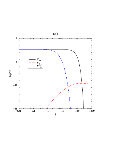
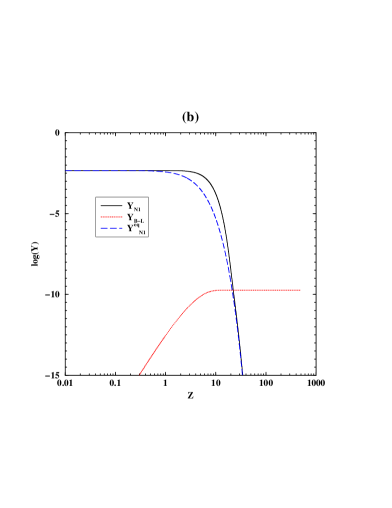
Figure 2.4: Dynamical evolution of neutrino number density in a comoving volume and the produced $B-L$ asymmetry at $M_{1}=10^{10}GeV$ and $\epsilon_{1}=-5\times 10^{-8}$.

In fig. 2.4 (a) we have used $\tilde{m}_{1}=10^{-6}eV$. Far above the mass scale of $N_{1}$ (i.e. $Z\ll 1$) the $B-L$ asymmetry is zero. As the temperature falls (i.e. Z increases) the asymmetry builds up and finally it reaches a constant value $Y_{B-L}=2.6\times 10^{-10}$ when the wash out effects become negligible. On the other hand, in fig. 2.4 (b) we have used $\tilde{m}_{1}=10^{-4}eV$ and we get a smaller asymmetry $1.8\times 10^{-10}$. This is because of larger effective neutrino mass. Note that the wash out effects not only depend on $M_{1}$ but also $\tilde{m}_{1}$. Therefore, for a larger $\tilde{m}_{1}$ the wash out effects is more and thus we get effectively a smaller asymmetry.

We now introduce a new parameter $m_{*}$ to be called equilibrium neutrino mass. It is defined by [45]

$$m_{*}=\frac{\tilde{\Gamma}_{D}}{H},$$ (2.39)

where

$$\tilde{\Gamma}_{D}=\frac{1}{16\pi v^{2}}\tilde{m}_{1}M_{1}^{2}$$ (2.40)

is obtained from equation (2.26) in the limit $Z\rightarrow\infty$ and $H$ is the Hubble expansion parameter. At any epoch of temperature $T$, the Hubble expansion parameter is defined as

$$H=1.67g_{*}^{1/2}\frac{T^{2}}{M_{pl}}.$$ (2.41)

Using (2.41) in equation (2.39) we get the equilibrium mass at $T\sim M_{1}$ to be

$$m_{*}=16\pi g_{*}^{1/2}\frac{G_{N}^{1/2}}{\sqrt{2}G_{F}}\simeq 2\times 10^{-3}eV,$$ (2.42)

where $G_{N}$ and $G_{F}$ are Newton and Fermi constants respectively and therefore $m_{*}$ may also be called cosmological neutrino mass [43].

We now define a dimensionless parameter $K=\frac{\tilde{m}_{1}}{m_{*}}$, which determines whether the species $N_{1}$ is in thermal equilibrium. For $K>1$, the inverse decay processes are fast enough to ensure the species $N_{1}$ to be in equilibrium, irrespective of its initial abundance, in the epoch $Z\rightarrow 0$ ($T\rightarrow\infty$). In this regime, any pre-existing asymmetry gets erased by the rapid inverse decay processes. Therefore, it is called strong wash out regime [28]. In this case the final lepton asymmetry doesn’t depend on the initial conditions (2.38). On the other hand, if $K\leq 1$, then the inverse decay processes are suppressed and the abundance of $N_{1}$ is not brought to equilibrium even for $Z\rightarrow 0$. In this case, any pre-existing asymmetry produced at the B-L symmetry breaking scale continue to be as it is until it gets some comparable contribution from the decays of $N_{1}$. So this regime is called weak wash out regime. In this regime the final lepton asymmetry strongly depends on the initial conditions.

In the following we study the solution of Boltzmann equations (2.23) and (2.24) by taking the zero initial abundance of $N_{1}$ for two different values of $\tilde{m}_{1}$ in the case $K\leq 1$. For the numerical solution we assume that

$$Y^{in}_{N1}=0~{}~{}{\mathrm{a}nd}~{}~{}Y^{in}_{B-L}=0$$ (2.43)

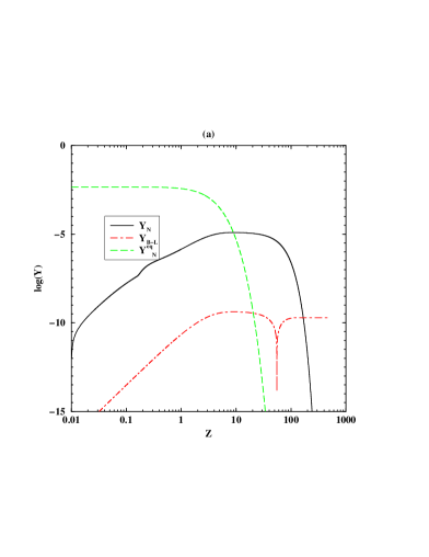
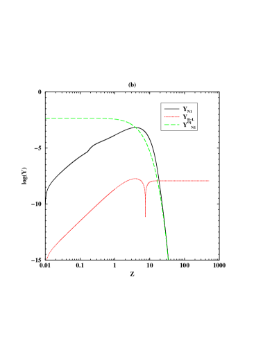
Figure 2.5: Dynamical evolution of neutrino number density for $K\leq 1$ and $Y_{N_{1}}^{in}=0$ along with the produced $B-L$ asymmetry at $M_{1}=10^{10}GeV$ and $\epsilon_{1}=-5\times 10^{-5}$.

In the figure 2.5(a) we have used $\tilde{m}_{1}=10^{-6}eV$, which is three orders of magnitude less than the equilibrium mass, $m_{*}\simeq O(10^{-3})eV$ of the light neutrino. In this scenario, the lightest right handed neutrino $N_{1}$ decays being out of equilibrium through out the evolution. Hence the erasure any pre-existing $L$-asymmetry is prevented. This remark is relevant to our study in chapter 4. On the other hand, in figure 2.5(b) we have used a larger $\tilde{m}_{1}=10^{-4}eV$, which is one order of magnitude less than $m_{*}$. Therefore, the neutrino abundance reaches the equilibrium value at an earlier time than the previous case.

Similar calculations are done for the case $K>1$ [28]. It is shown that the species $N_{1}$ is brought to equilibrium quickly even if we start with the zero abundance of $N_{1}$, and hence erasing any pre-existing asymmetry, in the epoch $Z\rightarrow 0$.

Chapter 3 Thermal leptogenesis in type-II seesaw models and bounds on neutrino masses

3.1 Introduction

In the type-I seesaw models the upper left $3\times 3$ block of the $6\times 6$ neutrino mass matrix is zero; see e.g., section 2.2. This is because of the absence of $\nu_{L}-\nu_{L}$ interaction in the $SM$ Lagrangian as it violates the lepton number by two units. In contrast to it, in type-II seesaw models the presence of an additional scalar triplet $\Delta_{L}$ allows us to add a $\nu_{L}-\nu_{L}$ interaction to the $SM$ Lagrangian by compensating the two units of $B-L$ charge appearing in the $\nu_{L}-\nu_{L}$ interaction term. At a low scale the $\Delta_{L}$ acquires a $VEV$, thus providing an additional mass $M_{L}=f\langle\Delta_{L}\rangle$, $f$ being the Majorana Yukawa coupling, to the light neutrino mass eigenstate through the diagonalization of the $6\times 6$ neutrino mass matrix. As a result the light neutrino mass matrix takes the form $m_{\nu}=M_{L}-m_{D}^{2}/M_{R}$. The two terms are called type-II and type-I respectively. The class of models in which both type-I and type-II terms occurring in $m_{\nu}$ are called type-II seesaw models.

3.2 Type-II seesaw mechanism and neutrino masses

In the minimal scenario, to achieve the light neutrino masses via the type-II seesaw mechanism, a scalar triplet $\Delta_{L}$ and a right handed Majorana neutrino per family are added to the $SM$. Thus the Lagrangian of this model reads

$$\mathcal{L}=\mathcal{L}_{SM}+\mathcal{L}_{new}\,$$ (3.1)

where $\mathcal{L}_{SM}$ is the $SM$ Lagrangian and $\mathcal{L}_{new}$ is the additional Lagrangian that contains the new interaction involving the right handed neutrinos and the triplet $\Delta_{L}$. The relevant terms of the Lagrangian are given to be

$$-\mathcal{L}_{new} \ni \frac{1}{2}M_{Ri}N_{Ri}^{T}CN_{Ri}+M_{\Delta}^{2}Tr\Delta_{L}^{\dagger}\Delta_{L}+h_{ij}\bar{\ell}_{i}\phi\bar{N}_{Rj}$$ (3.2)

$$+ f_{ij}\ell^{T}Ci\tau_{2}\Delta\ell_{j}-\mu\phi^{T}i\tau_{2}\Delta_{L}\phi+H.C.\,$$

where $\ell^{T}=(\nu_{Li},e_{Li})$ and $\phi^{T}=(\phi^{0},\phi^{-})$ and

$$\Delta_{L}=\begin{pmatrix}\frac{1}{\sqrt{2}}\delta^{+}&\delta^{++}\\ \delta^{0}&-\frac{1}{\sqrt{2}}\delta^{+}\end{pmatrix}.$$ (3.3)

In the presence of these interactions, the neutral component of the triplet acquires a $VEV$,

$$\langle\Delta_{L}\rangle=\begin{pmatrix}0&0\\ v_{L}&0\end{pmatrix},$$ (3.4)

at a scale much below the electroweak symmetry breaking phase transition. Due to this $VEV$ there are now in general two sources of light neutrino masses

$$m_{\nu} = fv_{L}-v^{2}hM_{R}^{-1}h^{T}$$ (3.5)

$$= m_{\nu}^{II}+m_{\nu}^{I}.$$

Note that $m_{\nu}^{II}$ that contribute to the neutrino mass matrix in the present case was absent in type-I models.

We can diagonalize the light neutrino mass matrix $m_{\nu}$, through lepton flavor mixing matrix $U_{L}$ [61]. This gives us three light Majorana neutrinos of masses

$$U_{L}^{T}m_{\nu}U_{L}=dia(m_{1},m_{2},m_{3})\equiv D_{m},$$ (3.6)

where the masses $m_{1},m_{2}$ and $m_{3}$ can be chosen to be real and positive.

3.3 Thermal leptogenesis in type-II seesaw models

In the type-II seesaw models the following decay modes:

$$\Delta\rightarrow\left\{\begin{array}[]{lr}\ell+\ell\\ \phi^{\dagger}+\phi^{\dagger}\end{array}\right.$$

and

$$N\rightarrow\left\{\begin{array}[]{lr}\bar{\ell}+\phi\\ \ell+\phi^{\dagger}\end{array}\right.$$

violate lepton number by two units and hence produce the lepton asymmetry. In the above equations $\ell$ and $\phi$ are $SM$ lepton and Higgs.

In what follows we assume a normal mass hierarchy in the heavy Majorana neutrino sector. We also assume that the quartic self coupling of the $SM$ Higgs, which is expected to be of order unity, is much larger than the Majorana Yukawa coupling of lightest right handed heavy Majorana neutrino $N_{1}$. In this case while the heavier right handed neutrinos, $N_{2}$ and $N_{3}$ and the triplet $\Delta_{L}$ decay, the lightest of heavy Majorana neutrinos is still in thermal equilibrium. Any asymmetry thus produced by the decay of $N_{2}$, $N_{3}$ and $\Delta_{L}$ will be erased by the lepton number violating interactions mediated by $N_{1}$. Therefore, it is reasonable to assume that the final lepton asymmetry is given only by the $CP$-violating decays of $N_{1}$ to the $SM$ fields $\ell$ and $\phi$.

3.3.1 Upper bound on $CP$-asymmetry

In comparison to the $CP$-asymmetry (2.8) in type-I models there is an additional contribution  [65, 66] in type-II seesaw models due to the one loop radiative correction through the virtual triplet $\Delta_{L}$ in the decays of lightest right handed Majorana neutrino. We assume that the masses of $\Delta_{L}$, $N_{2}$ and $N_{3}$ are much heavier than the the mass scale of $N_{1}$. In this scenario the total $CP$-asymmetry is given by

$$\epsilon_{1}=\epsilon_{1}^{I}+\epsilon_{1}^{II},$$ (3.7)

where the contribution to $\epsilon_{1}^{I}$ comes from the interference of tree level, self-energy correction and the one loop radiative correction diagrams involving the heavier Majorana neutrinos $N_{2}$ and $N_{3}$. This contribution is the same as in type-I models [27, 28] and is given by

$$\epsilon_{1}^{I}=\frac{3M_{1}}{16\pi v^{2}}\frac{\sum_{i,j}Im\left[(h^{\dagger})_{1i}(m_{\nu}^{I})_{ij}(h^{*})_{j1}\right]}{(h^{\dagger}h)_{11}}.$$ (3.8)

Figure 3.1: One loop radiative correction through the virtual triplet $\Delta_{L}$.

On the other hand the contribution to $\epsilon_{1}^{II}$ in equation (3.7) comes from the interference of tree level diagram and the one loop radiative correction diagram involving the triplet $\Delta_{L}$ as shown in fig. 3.1. It is given by [31, 67]

$$\epsilon_{1}^{II}=\frac{3M_{1}}{16\pi v^{2}}\frac{\sum_{i,j}Im\left[(h^{\dagger})_{1i}(m_{\nu}^{II})_{ij}(h^{*})_{j1}\right]}{(h^{\dagger}h)_{11}}.$$ (3.9)

Substituting (3.8) and (3.9) in equation (3.7) and using (3.5), we get the total CP-asymmetry

$$\epsilon_{1}=\frac{3M_{1}}{16\pi v^{2}}\frac{Im(h^{\dagger}m_{\nu}h^{*})_{11}}{(h^{\dagger}h)_{11}}.$$ (3.10)

Using (3.6) in equation (3.10) we get

$$\epsilon_{1} = \frac{3M_{1}}{16\pi v^{2}}\frac{Im(h^{\dagger}U_{L}^{*}D_{m}U_{L}^{\dagger}h^{*})_{11}}{(h^{\dagger}h)_{11}}$$ (3.11)

$$= \frac{3M_{1}}{16\pi v^{2}}\frac{\sum_{i}m_{i}Im[(U_{L}^{T}h)_{i1}^{*}]^{2}}{\sum_{i}|(U_{L}^{T}h)_{i1}|^{2}}.$$

With an assumption of normal mass hierarchy for the light Majorana neutrinos the upper bound on $CP$-asymmetry (3.11) can be given by

$$\epsilon_{1}\leq\frac{3M_{1}}{16\pi v^{2}}m_{3}.$$ (3.12)

Note that the above upper bound (3.12) for $\epsilon_{1}$ as a function of $M_{1}$ and $m_{3}$ was first obtained for the case of type-I seesaw models [27]. However, the same relation holds in the case of type-II seesaw models also [31] independent of the relative magnitudes of $m_{\nu}^{I}$ and $m_{\nu}^{II}$.

3.3.2 Estimation of $L$-asymmetry and lower bound on the mass of lightest right handed neutrino

Assuming $M_{1}\ll M_{2}$, $M_{3}$, $M_{\Delta}$, the final lepton asymmetry is given by the out of equilibrium decays of the lightest right handed Majorana neutrino $N_{1}$. A part of this asymmetry is then transformed to $B$-asymmetry by the thermally equilibrated sphaleron processes which violate $B+L$ quantum number of $SM$ fermions. In a comoving volume a net $B$-asymmetry can be written as

$$Y_{B}=\frac{n_{B}}{s}=0.55\epsilon_{1}Y_{N_{1}}\delta,$$ (3.13)

where the factor 0.55 in front [44] is the fraction of $L$-asymmetry that is converted to $B$-asymmetry. Here $Y_{N_{1}}$ is the density of $N_{1}$ in a comoving volume which is given by $Y_{N_{1}}=n_{N_{1}}/s$, $s$ being the entropy density of the Universe at any epoch of temperature $T$ and $\delta$ is the wash out factor.

We now recast equation (3.13) in terms of a measurable quantity $(n_{B}/n_{\gamma})$ which is given by

$$\left(\frac{n_{B}}{n_{\gamma}}\right)=7(Y_{B})=3.85(\epsilon_{1}Y_{N_{1}}\delta).$$ (3.14)

Substituting equation (3.12) in (3.14) we get a bound on the baryon asymmetry to be

$$\left(\frac{n_{B}}{n_{\gamma}}\right)\leq 3.85\left(\frac{3M_{1}}{16\pi v^{2}}\right)m_{3}Y_{N_{1}}\delta.$$ (3.15)

Using (2.15) in equation (3.15) and comparing with the observed baryon asymmetry (2.20) we get a bound on the mass of $N_{1}$ to be

$$M_{1}\geq 0.84\times 10^{8}GeV\left(\frac{10^{-2}}{Y_{N_{1}}\delta}\right)\left(\frac{0.05eV}{m_{3}}\right).$$ (3.16)

This bound was obtained in type-I seesaw models. However, in this case we revisit the same bound on the mass of $N_{1}$ irrespective of any assumption regarding the magnitude of type-I and type-II terms in the neutrino mass matrix (3.5).

3.4 Spontaneous $CP$-violation and leptogenesis in Left-Right symmetric models

In section 3.2 we demonstrated the type-II seesaw mechanism in a minimal scenario by adding a right handed Majorana neutrino per generation and a heavy triplet $\Delta_{L}$ to the $SM$. However, the light neutrino masses via type-II seesaw mechanism can be obtained naturally in Left-Right or $SO(10)$ models. In the following we consider the low energy left-right symmetric model in which we assume the case of spontaneous $CP$-violation ($SCPV$). In this scenario we derive an upper bound on the $CP$-asymmetry. Moreover, we discuss the bounds on neutrino masses from the leptogenesis constraint.

3.4.1 Left-Right symmetric model and $SCPV$

In the low energy left-right symmetric model the right handed charged lepton of each family, which was a singlet under the $SM$ gauge group $SU(2)_{L}\otimes U(1)_{Y}$, gets a new partner $\nu_{R}$. These two form a doublet under the $SU(2)_{R}$ of the left-right symmetric gauge group $SU(2)_{L}\otimes SU(2)_{R}\otimes U(1)_{B-L}$. Similarly, in the quark sector, the right handed up and down quarks of each family, which were singlets under $SM$ gauge group, combine to form a doublet under $SU(2)_{R}$.

The Higgs sector of the model is dictated by two triplets $\Delta_{L}$ and $\Delta_{R}$ and a bidoublet $\Phi$, which contains two copies of $SM$ Higgs. Under $SU(2)_{L}\otimes SU(2)_{R}\otimes U(1)_{B-L}$ the field content and the quantum numbers of the Higgs fields are given as

$$\Phi = \begin{pmatrix}\phi_{1}^{0}&\phi_{1}^{+}\\ \phi_{2}^{-}&\phi_{2}^{0}\end{pmatrix}\sim(1/2,1/2,0)$$ (3.17)

$$\Delta_{L} = \begin{pmatrix}\delta_{L}^{+}/\sqrt{2}&\delta_{L}^{++}\\ \delta_{L}^{0}&-\delta_{L}^{+}/\sqrt{2}\end{pmatrix}\sim(1,0,2)$$ (3.18)

$$\Delta_{R} = \begin{pmatrix}\delta_{R}^{+}/\sqrt{2}&\delta_{R}^{++}\\ \delta_{R}^{0}&-\delta_{R}^{+}/\sqrt{2}\end{pmatrix}\sim(0,1,2).$$ (3.19)

To achieve the correct phenomenology, the various Higgs multiplets in the model should have the following VEVs,

$$\langle\Delta_{R}\rangle=\begin{pmatrix}0&0\\ v_{R}e^{i\theta_{R}}&0\end{pmatrix},$$ (3.20)

$$\langle\Phi\rangle=\begin{pmatrix}k_{1}e^{i\alpha}&0\\ 0&k_{2}e^{i\beta}\end{pmatrix},$$ (3.21)

and

$$\langle\Delta_{L}\rangle=\begin{pmatrix}0&0\\ v_{L}e^{i\theta_{L}}&0\end{pmatrix}.$$ (3.22)

The electric charge of the fields is given by

$$Q=T^{3}_{L}+T^{3}_{R}+\frac{1}{2}(B-L).$$ (3.23)

In the above $v_{L}$, $v_{R}$, $k_{1}$ and $k_{2}$ are real parameters and the electroweak symmetry breaking scale $v=174$ GeV is given by $v^{2}=k_{1}^{2}+k_{2}^{2}$. Further we require that $v_{L}\ll v\ll v_{R}$. The requirement of the spontaneous breakdown of parity gives rise to

$$v_{L}v_{R}=\gamma(k_{1}^{2}+k_{2}^{2})=\gamma v^{2},$$ (3.24)

where $\gamma$ is parameter which is a function of the quartic couplings in the Higgs potential.

The minimisation of the most general Higgs potential involving $\Delta_{L},\Delta_{R}$ and $\Phi$ was studied in refs. [34]. The relations between the various couplings, for which the above set of VEVs are generated, were derived. In this scenario, the gauge symmetry $SU(2)_{L}\times SU(2)_{R}\times U(1)_{B-L}$ is broken to $U(1)_{em}$ in a single step. Thus the $CP$-violating phases come into existence at the same scale where the left-right symmetry is broken. Since $v\ll v_{R}$, the $SM$ symmetry is present as an approximate symmetry at the scale where symmetry breaking occurs.

The fermions get their masses via Yukawa couplings. The Lagrangian for one generation of quarks and leptons is

$$-\mathcal{L}_{yuk} = \tilde{h}_{q}\bar{q}_{L}\Phi q_{R}+\tilde{g}_{q}\bar{q}_{L}\tilde{\Phi}q_{R}+\tilde{h}_{l}\bar{\ell}_{L}\Phi l_{R}+\tilde{g}_{l}\bar{\ell}_{L}\tilde{\Phi}l_{R}$$ (3.25)

$$+if(\ell_{L}^{T}C\tau_{2}\Delta_{L}\ell_{L}+\ell_{R}^{T}C\tau_{2}\Delta_{R}\ell_{R})+H.c.\,$$

where $q$ and $\ell$ are quark and lepton doublets, $\tilde{\Phi}=\tau_{2}\Phi^{*}\tau_{2}$ and $C$ is the Dirac charge conjugation matrix. Further the Majorana Yukawa coupling $f$ is the same for both left and right handed neutrinos to maintain the discrete $L\leftrightarrow R$ symmetry.

Substituting the complex $VEV$s (3.20), (3.21) and (3.22) in (3.25) we obtain fermion mass terms to be

$$\mathcal{L}_{mass} = (\tilde{h}_{q}k_{1}e^{i\alpha}+\tilde{g}_{q}k_{2}e^{i\beta})\bar{u}_{L}u_{R}+(\tilde{h}_{q}k_{2}e^{i\beta}+\tilde{g}_{q}k_{1}e^{i\alpha})\bar{d}_{L}d_{R}$$ (3.26)

$$+(\tilde{h}_{l}k_{1}e^{i\alpha}+\tilde{g}_{l}k_{2}e^{i\beta})\bar{\nu}_{L}\nu_{R}+(\tilde{h}_{l}k_{2}e^{i\beta}+\tilde{g}_{l}k_{1}e^{i\alpha})\bar{e}_{L}e_{R}$$

$$+f(\nu_{L}^{T}Cv_{L}e^{i\theta_{L}}\nu_{L}+\nu_{R}^{T}Cv_{R}e^{i\theta_{R}}\nu_{R})+H.C.$$

Generalizing the above equation (3.26) for three generation of matter fields we get the up and down quark mass matrices to be

$$(M_{u})_{ij}=(\tilde{h}_{q})_{ij}k_{1}e^{i\alpha}+(\tilde{g}_{q})_{ij}k_{2}e^{i\beta}~{}~{}\mathrm{and}~{}~{}(M_{d})_{ij}=(\tilde{h}_{q})_{ij}k_{2}e^{i\beta}+(\tilde{g}_{q})_{ij}k_{1}e^{i\alpha}.$$ (3.27)

We assume [34, 68] $k_{1}/k_{2}\sim m_{t}/m_{b}$. In the seesaw mechanism, the Dirac mass matrix of the neutrinos is assumed to be similar to the mass matrix of the charged leptons. For $k_{2}\ll k_{1}$, and further assuming $\tilde{h}_{l}\sim\tilde{g}_{l}$ in (3.26), the Dirac mass matrix of the neutrinos to a good approximation becomes $\tilde{h}_{l}k_{1}e^{i\alpha}$. Thus neglecting $k_{2}$ terms, the masses of three generations of neutrinos are given by

$$\mathcal{L}_{\nu-mass}=\bar{\nu}_{L_{i}}k_{1}e^{i\alpha}(\tilde{h}_{l})_{ij}\nu_{R_{j}}+f_{ij}(v_{L}e^{i\theta_{L}}\nu_{L_{i}}^{T}C\nu_{L_{j}}+v_{R}e^{i\theta_{R}}\nu_{R_{i}}^{T}C\nu_{R_{j}})+H.C.$$ (3.28)

The Majorana mass matrix for the right handed neutrinos can be diagonalized by making the following orthogonal transformation on $\nu_{R}$

$$N_{R}=O_{R}^{T}\nu_{R}.$$ (3.29)

In this basis, we have

$$O_{R}^{T}fO_{R} = f_{dia},$$ (3.30)

$$h = \tilde{h}O_{R}.$$ (3.31)

In the transformed basis we get the mass matrix for the neutrinos

$$\begin{pmatrix}fv_{L}e^{i\theta_{L}}&k_{1}e^{i\alpha}h\\ k_{1}e^{i\alpha}h^{T}&f_{dia}v_{R}e^{i\theta_{R}}\end{pmatrix}.$$ (3.32)

Diagonalizing the neutrino mass matrix into $3\times 3$ blocks we get the light neutrino mass matrix to be

$$m_{\nu}=fv_{L}e^{i\theta_{L}}-\frac{k_{1}^{2}}{v_{R}}(hf_{dia}^{-1}h^{T})e^{i(2\alpha-\theta_{R})}$$ (3.33)

Notice that the Lagrangian (3.25) is invariant under the following unitary transformations of the fermion and Higgs fields,

$$\psi_{L}\longrightarrow U_{L}\psi_{L}~{}~{} \mathrm{and}~{}~{} \psi_{R}\longrightarrow U_{R}\psi_{R},$$ (3.34)

$$\Phi\longrightarrow U_{L}\Phi U_{R}^{\dagger}~{}~{} \mathrm{and}~{}~{} \tilde{\Phi}\longrightarrow U_{L}\tilde{\Phi}U_{R}^{\dagger}$$ (3.35)

$$\Delta_{L}\longrightarrow U_{L}\Delta_{L}U_{L}^{\dagger}~{}~{} \mathrm{and}~{}~{} \Delta_{R}\longrightarrow U_{R}\Delta_{R}U_{R}^{\dagger},$$ (3.36)

where $\psi_{L,R}$ is a doublet of quark or lepton fields. The invariance under $U_{L}$ is the result of the remnant global $U(1)$ symmetry which remains after the breaking of the gauge symmetry $SU(2)_{L}$ and similarly for $U_{R}$. The matrices $U_{L}$ and $U_{R}$ can be parametrized as

$$U_{L}=\begin{pmatrix}e^{i\gamma_{L}}&0\\ 0&e^{-i\gamma_{L}}\end{pmatrix}~{}~{}\mathrm{and}~{}~{}U_{R}=\begin{pmatrix}e^{i\gamma_{R}}&0\\ 0&e^{-i\gamma_{R}}\end{pmatrix}.$$ (3.37)

By redefining the phases of the fermion fields we can rotate away two of the phase degrees of freedom from the scalar sector of the theory. Thus only two of the four phases of Higgs $VEV$s have phenomenological consequences. Under these unitary transformations, the $VEV$s (3.20), (3.21) and (3.22) become

$$\langle\Delta_{R}\rangle=\begin{pmatrix}0&0\\ v_{R}e^{i(\theta_{R}-2\gamma_{R})}&0\end{pmatrix},$$ (3.38)

$$\langle\Phi\rangle=\begin{pmatrix}k_{1}e^{i(\alpha+\gamma_{L}-\gamma_{R})}&0\\ 0&k_{2}e^{i(\beta-\gamma_{L}+\gamma_{R})}\end{pmatrix},$$ (3.39)

and

$$\langle\Delta_{L}\rangle=\begin{pmatrix}0&0\\ v_{L}e^{i(\theta_{L}-2\gamma_{L})}&0\end{pmatrix}.$$ (3.40)

We choose $\gamma_{R}=\theta_{R}/2$ so that the masses of the right handed neutrinos are real. The light neutrino mass matrix (3.33) then becomes

$$m_{\nu} = fv_{L}e^{i(\theta_{L}-2\gamma_{L})}-\frac{k_{1}^{2}}{v_{R}}(hf_{dia}^{-1}h^{T})e^{i(2\alpha+2\gamma_{L}-\theta_{R})}$$ (3.41)

$$= m_{\nu}^{II}+m_{\nu}^{I}$$ (3.42)

Conventionally, in equation (3.41), $\gamma_{L}$ was chosen to be $-\alpha+\theta_{R}/2$  [34, 69]. This makes $m_{\nu}^{I}$ real leaving the imaginary part purely in $m_{\nu}^{II}$. We call this type-II phase choice. The light neutrino mass matrix, with this phase choice, is

$$m_{\nu}=fv_{L}e^{i\theta^{\prime}_{L}}-\frac{k_{1}^{2}}{v_{R}}(hf_{dia}^{-1}h^{T}),$$ (3.43)

where $\theta^{\prime}_{L}=(\theta_{L}-\theta_{R}+2\alpha)$. On the other hand, by choosing $\gamma_{L}=\theta_{L}/2$ in equation (3.41) $m_{\nu}^{II}$ can be made real, with the phase occurring purely in $m_{\nu}^{I}$. We call this type-I phase choice. Consequently the light neutrino mass matrix (3.41) becomes

$$m_{\nu}=fv_{L}-\frac{k_{1}^{2}}{v_{R}}e^{i\theta^{\prime}_{R}}(hf_{dia}^{-1}h^{T})\,$$ (3.44)

where $\theta^{\prime}_{R}=(\theta_{L}-\theta_{R}+2\alpha)$. The $CP$-violating parameter $\epsilon_{1}$ which gives rise to the lepton asymmetry is independent of the phase choice. However, the theoretical upper bound on $\epsilon_{1}$ is not a physical parameter of the theory and can depend on the choice of phases as we see in the next section. In numerical calculations, we take into account the consistency of the bounds coming from the different phase choices.

Using (3.6) we can diagonalize the light neutrino mass matrix $m_{\nu}$. This gives us three eigenvalues, $m_{1}$, $m_{2}$ and $m_{3}$ which are chosen to be real.

3.4.2 Upper bound on $CP$-asymmetry in Left-Right symmetric models with $SCPV$

Following the same convention in section 3.3.1 we can write the total $CP$-asymmetry in Left-Right symmetric model as

$$\epsilon_{1}=\frac{3M_{1}}{16\pi v^{2}}\frac{\sum_{i,j}Im\left[h^{T}_{1i}(m_{\nu}^{I}+m_{\nu}^{II})_{ij}h_{j1}\right]}{(h^{T}h)_{11}}.$$ (3.45)

From equation (3.45), we see that the physical observable $\epsilon_{1}$ is not affected by the choice of phases. In the following, we use bound on $\epsilon_{1}$ from the observed baryon asymmetry to obtain bounds on right-handed neutrino masses for the two different phase choices.

A. The type-II choice of phases

In this choice of phases the type-I mass term is real. The only source of $CP$-violation in the light neutrino mass matrix $m_{\nu}$ lies in the type-II mass term. Thus in this case $\epsilon_{1}^{I}=0$ because of both h and $m_{\nu}^{I}$ are real. The total $CP$-asymmetry in this choice of phases is therefore given by

$$\epsilon_{1} = \epsilon_{1}^{II}$$ (3.46)

$$= \frac{3M_{1}v_{L}}{16\pi v^{2}}\frac{(h^{T}fh)_{11}}{(h^{T}h)_{11}}Im(e^{i\theta^{\prime}_{L}}).$$

Using (3.30) and (3.31) in equation (3.46) we get

$$\epsilon_{1}=\frac{3M_{1}v_{L}}{16\pi v^{2}}\frac{\sum_{i}f_{i}(O_{R}^{T}h)_{i1}^{2}}{\sum_{i}(O_{R}^{T}h)_{i1}^{2}}sin\theta^{\prime}_{L},$$ (3.47)

where $f_{i}=(M_{i}/v_{R})$. Up to a first order approximation it is reasonable to assume that $\sum_{i}f_{i}\approx 1$. In this approximation the maximum value of the $CP$-asymmetry (3.47) is given by [27, 28, 31, 32]

$$\epsilon_{1,max}=\frac{3M_{1}v_{L}}{16\pi v^{2}}.$$ (3.48)

Thus, for type-II phase choice, a bound on $\epsilon_{1}$ leads to a bound on $M_{1}$.

B. The type-I choice of phases

In the type-I choice of phases the type-II mass term is real. Hence the $CP$-violation comes through the type-I mass term only. The total $CP$-asymmetry in this case is therefore given by

$$\epsilon_{1} = \epsilon_{1}^{I}$$ (3.49)

$$= \frac{3M_{1}k_{1}^{2}}{16\pi v^{2}v_{R}}\frac{(h^{T}hf_{dia}^{-1}h^{T}h)_{11}}{(h^{T}h)_{11}}Im(e^{-i\theta_{R}^{\prime}}).$$

Let us consider the type-I term of the light neutrino mass matrix

$$m_{\nu}^{I} = m_{\nu}-m_{\nu}^{II}$$ (3.50)

$$= -\frac{k_{1}^{2}}{v_{R}^{\prime}}hf_{dia}^{-1}h^{T},$$

where $v^{\prime}_{R}=v_{R}e^{i\theta_{R}^{\prime}}$. We can find a diagonalizing matrix $U={\cal{O}}U_{phase}$ for $m_{\nu}^{I}$ such that

$$U^{T}m_{\nu}^{I}U\equiv-D_{m_{I}}=-dia(m_{I_{1}},m_{I_{2}},m_{I_{3}})$$ (3.51)

where $m_{I_{1}},m_{I_{2}}$ and $m_{I_{3}}$ are made real by choosing $U_{phase}=e^{i\theta_{R}^{\prime}/2}$. Therefore, from equation (3.51) we have

$$D_{m_{I}}=\frac{k_{1}^{2}}{v_{R}}{\cal{O}}^{T}\left(hf_{dia}^{-1}h^{T}\right){\cal{O}}.$$ (3.52)

Using (3.52) in equation (3.49) the $CP$-asymmetry $\epsilon_{1}$ can be rewritten as

$$\epsilon_{1} = \frac{3M_{1}}{16\pi v^{2}}\frac{\sum_{i}\left[(h^{T}{\cal{O}})_{1i}D_{m_{I_{ii}}}({\cal{O}}^{T}h)_{i1}\right]}{\sum_{i}\left[(h^{T}{\cal{O}})_{1i}({\cal{O}}^{T}h)_{i1}\right]}Im(e^{-i\theta_{R}^{\prime}})$$ (3.53)

$$= \frac{3M_{1}}{16\pi v^{2}}\frac{\sum_{i}m_{I_{i}}({\cal{O}}^{T}h)_{i1}^{2}}{\sum_{i}({\cal{O}}^{T}h)_{i1}^{2})}Im(e^{-i\theta_{R}^{\prime}}).$$

In the above equation (3.53) the maximum value of $CP$-asymmetry is thus given by [27, 28]

$$|\epsilon_{1,max}|=\frac{3M_{1}}{16\pi v^{2}}\sum_{i}m_{I_{i}}.$$ (3.54)

In the equation (3.54) $m_{I}$s are the eigenvalues of the matrix $m_{\nu}^{I}$ and are not the physical light neutrino masses. It is desirable to express the $\epsilon_{1,max}$ in terms of physical parameters. In order to calculate the $m_{I}$s we will assume a hierarchical texture of Majorana coupling

$$f_{dia}=\frac{M_{1}}{v_{R}}\begin{pmatrix}1&0&0\\ 0&\alpha_{A}&0\\ 0&0&\alpha_{B}\end{pmatrix},$$ (3.55)

where $1\ll\alpha_{A}=(M_{2}/M_{1})\ll\alpha_{B}=(M_{3}/M_{1})$. We identify the neutrino Dirac Yukawa coupling $h$ with that of charged leptons [18]. We assume $h$ to be of Fritzsch type [70]

$$h=\frac{(m_{\tau}/v)}{1.054618}\begin{pmatrix}0&a&0\\ a&0&b\\ 0&b&c\end{pmatrix}.$$ (3.56)

We make this assumption because Fritzsch mass matrices are well motivated phenomenologically. By choosing the values of $a$, $b$ and $c$ suitably one can get the hierarchy for charged leptons and quarks. In particular  [70]

$$a=0.004,~{}~{}~{}b=0.24~{}~{}~{}{\rm and}~{}~{}~{}c=1$$ (3.57)

can give the mass hierarchy of charged leptons. For this set of values the mass matrix $h$ is normalized with respect to the $\tau$-lepton mass. The set of values of $a$, $b$ and $c$ are roughly in geometric progression. They can be expressed in terms of the electro-weak gauge coupling $\alpha_{w}=\frac{g^{2}}{4\pi}=\frac{\alpha}{sin^{2}\theta_{w}}$. In particular $a=2.9\alpha_{w}^{2}$, $b=6.5\alpha_{w}$ and $c=1$. Here onwards we will use these set of values for the parameters of $h$. Using equation (3.55) and (3.56) in equation (3.52), we now get

$$D_{mI} = \frac{v^{2}}{v_{R}}\left(hf_{dia}^{-1}h^{T}\right)_{dia}$$ (3.58)

$$\simeq \frac{v^{2}}{M_{1}}\frac{(m_{\tau}/v)^{2}}{(1.054618)^{2}}\begin{pmatrix}0&0&0\\ 0&A&0\\ 0&0&B\end{pmatrix},$$

where the eigenvalues $A$ and $B$ are functions of $\alpha_{A}$ and $\alpha_{B}$ and their sum is given by

$$A+B=\frac{1}{2}\left[a^{2}+\frac{1}{\alpha_{A}}(a^{2}+b^{2})+\frac{1}{\alpha_{B}}(b^{2}+c^{2})\right].$$ (3.59)

Using equation (3.58) we can write the maximum value of $CP$-asymmetry (3.54)

$$\epsilon_{1,max} = \frac{3M_{1}}{16\pi v^{2}}(m_{I2}+m_{I3})$$ (3.60)

$$= \frac{3}{16\pi}\frac{(m_{\tau}/v)^{2}}{(1.054618)^{2}}(A+B).$$

Thus we see that, in type-I choice of phases, the leptogenesis parameter $\epsilon_{1}$ constrains the hierarchy parameters $\alpha_{A}$ and $\alpha_{B}$. In the following two sections, we will obtain numerical bounds on $\alpha_{A}$ and $\alpha_{B}$ in a manner consistent with the bound $M_{1}$ coming from the type-II phase choice.

3.4.3 Estimation of $L$-asymmetry and bound on neutrino masses

A net $B-L$ asymmetry is generated when left-right symmetry breaks. A partial $B-L$ asymmetry is then gets converted to $B$-asymmetry by the high temperature sphaleron transitions. However these sphaleron fields conserve $B-L$. Therefore, the produced $B-L$ asymmetry will not be washed out, rather they will keep on changing it to $B$-asymmetry. Thus in a comoving volume a net $B$-asymmetry is given by

$$Y_{B}=\frac{n_{B}}{s}=\frac{28}{79}\epsilon_{1}Y_{N1}\delta,$$ (3.61)

where the factor $\frac{28}{79}$ in front [44] is the fraction of $B-L$ asymmetry that gets converted to $B$-asymmetry. Here $\epsilon_{1}$ is given by equation (3.60). The other symbols involved in equation (3.61) carry the usual meaning; see, e.g. section 3.3.2. However, the observed baryon asymmetry of the Universe is measured in terms of $n_{B}/n_{\gamma}$. Therefore, we rewrite equation (3.61) as

$$\left(\frac{n_{B}}{n_{\gamma}}\right)=7(Y_{B})=2.48(\epsilon_{1}Y_{N}\delta).$$ (3.62)

Substituting the type-II phase choice relation (3.48) in (3.62) and comparing with the observed value (2.20) of the baryon asymmetry we get the bound on the mass of lightest right handed neutrino to be

$$M_{1}\geq 1.25\times 10^{8}GeV\left(\frac{10^{-2}}{Y_{N_{1}}\delta}\right)\left(\frac{0.1eV}{v_{L}}\right).$$ (3.63)

On the other hand, substitution of $\epsilon_{1,max}$ from the type-I phase choice (3.60) in equation (3.62) and then comparison with the observed value (2.20) gives the constraint

$$A+B\geq 3.46\times 10^{-3}(10^{-2}/Y_{N}\delta)\left(\frac{\left(n_{B}/n_{\gamma}\right)_{0}}{6.1\times 10^{-10}}\right)\left(\frac{2GeV}{m_{\tau}}\right)\left(\frac{v}{174GeV}\right)^{2},$$ (3.64)

where the physical quantities are normalized with respect to their observed values. The above equation, for the values of $a$, $b$ and $c$ from (3.57), gives only one constraint on the two hierarchy parameters $\alpha_{A}$ and $\alpha_{B}$. We will determine the individual parameters $\alpha_{A}$ and $\alpha_{B}$ by demanding that their values should reproduce the low energy neutrino parameters correctly, while satisfying the inequalities $M_{1}>O(10^{8})$ GeV and $\alpha_{B}>\alpha_{A}>>1$. Individual bounds on $\alpha_{A}$ and $\alpha_{B}$ can also be obtained if we assume that the $\alpha_{A}$ term and the $\alpha_{B}$ term in the sum $A+B$ from equation (3.59) are roughly equal. We then get

$$\alpha_{A}=(M_{2}/M_{1})\leq 17~{}~{}{\rm and}~{}~{}\alpha_{B}=(M_{3}/M_{1})\leq 289.$$ (3.65)

3.4.4 Checking the Consistency of $f$-matrix eigenvalues

The solar and atmospheric evidences of neutrino oscillations are nicely accommodated in the minimal framework of the three-neutrino mixing, in which the three neutrino flavors $\nu_{e}$, $\nu_{\mu}$, $\nu_{\tau}$ are unitary linear combinations of three neutrino mass eigenstates $\nu_{1}$, $\nu_{2}$, $\nu_{3}$ with masses $m_{1}$, $m_{2}$, $m_{3}$ respectively. The mixing among these three neutrinos determines the structure of the lepton mixing matrix [61] which can be parameterized as

$$U_{L}=\begin{pmatrix}c_{1}c_{3}&s_{1}c_{3}&s_{3}e^{i\delta}\\ -s_{1}c_{2}-c_{1}s_{2}s_{3}e^{i\delta}&c_{1}c_{2}-s_{1}s_{2}s_{3}e^{i\delta}&s_{2}c_{3}\\ s_{1}s_{2}-c_{1}c_{2}s_{3}&-c_{1}s_{2}-s_{1}c_{2}s_{3}e^{i\delta}&c_{2}c_{3}\end{pmatrix}dia(1,e^{i\alpha},e^{i(\beta+\delta)}),$$ (3.66)

where $c_{j}$ and $s_{j}$ stands for $\cos\theta_{j}$ and $\sin\theta_{j}$. The two physical phases $\alpha$ and $\beta$ associated with the Majorana character of neutrinos are not relevant for neutrino oscillations [71] and will be set to zero here onwards. While the Majorana phases can be investigated in neutrinoless double beta decay experiments [72], the CKM-phase $\delta\in[-\pi,\pi]$ can be investigated in long base line neutrino oscillation experiments. For simplicity we set it to zero, since we are interested only in the magnitudes of elements of $U_{L}$. The best fit values of the neutrino masses and mixings from a global three neutrino flavors oscillation analysis are  [73]

$$\theta_{1}=\theta_{\odot}\simeq 34^{\circ},~{}~{}\theta_{2}=\theta_{atm}=45^{\circ},~{}~{}\theta_{3}\leq 10^{\circ},$$ (3.67)

and

$$\Delta m_{\odot}^{2}=m_{2}^{2}-m_{1}^{2} \simeq m_{2}^{2}=7.1\times 10^{-5}\ {\rm eV}^{2}$$

$$\Delta m_{atm}^{2}=m_{3}^{2}-m_{2}^{2} \simeq m_{3}^{2}=2.6\times 10^{-3}\ {\rm eV}^{2}.$$ (3.68)

Using equation (3.33) we rewrite the $f$-matrix

$$f=(\frac{eV}{v_{L}})\left[(m_{\nu}/eV)+\frac{4}{(1.054165)^{2}}\frac{1}{(M_{1}/{\rm GeV})}\begin{pmatrix}\frac{a^{2}}{\alpha_{A}}&0&\frac{ab}{\alpha_{A}}\\ 0&a^{2}+\frac{b^{2}}{\alpha_{B}}&\frac{bc}{\alpha_{B}}\\ \frac{ab}{\alpha_{A}}&\frac{bc}{\alpha_{B}}&\frac{b^{2}}{\alpha_{A}}+\frac{c^{2}}{\alpha_{B}}\end{pmatrix}\right],$$ (3.69)

where the neutrino mass matrix $m_{\nu}$ is given by equation(3.6). The constrained eigenvalues $\alpha_{A}$ and $\alpha_{B}$ are given by equation (3.65).

In the following, we choose $M_{1}$ to be larger than the bound given by type-II phase choice (3.63) and $m_{1}$ such that $m_{1}^{2}<<\Delta_{sol}$. For such $m_{1}$ and $M_{1}$, we choose suitable $\alpha_{A}$ and $\alpha_{B}$ that are compatible with the low energy neutrino oscillation data. In particular here we choose $m_{1}=1.0\times 10^{-3}eV$, $M_{1}=1.0\times 10^{8}$ GeV, $\alpha_{A}=17$, $\alpha_{B}=170$ and $\theta_{3}=6^{\circ}$. Then we get

$$f_{dia}=\frac{2.16\times 10^{-3}eV}{v_{L}}\begin{pmatrix}1&0&0\\ 0&17.3&0\\ 0&0&169.7\end{pmatrix}.$$ (3.70)

Thus, for the above values of $m_{1}$ and $M_{1}$, the assumed hierarchy of right-handed neutrino masses is consistent with global low energy neutrino data. Comparing equation (3.70) with (3.55) we get

$$\frac{M_{1}}{v_{R}}=\frac{2.16\times 10^{-3}eV}{v_{L}}.$$ (3.71)

This implies that $v_{R}=O(10^{10})$ GeV for $v_{L}=0.1$ eV. These values of $v_{L}$ and $v_{R}$ are compatible with genuine seesaw $v_{L}v_{R}=\gamma v^{2}$ for a small value of $\gamma\simeq O(10^{-4})$ [74]. On the other hand, if we choose the parameters $m_{1}=1.0\times 10^{-3}$ eV, $M_{1}=1.0\times 10^{9}$ GeV, $\alpha_{A}=17$, $\alpha_{B}=65$ and $\theta_{3}=6^{\circ}$ we get

$$f_{dia}=\frac{1.6\times 10^{-3}eV}{v_{L}}\begin{pmatrix}1&0&0\\ 0&16.76&0\\ 0&0&64.68\end{pmatrix}.$$ (3.72)

Once again we have consistency between the assumed hierarchy of right-handed neutrino masses and global low energy neutrino data. Again comparing equation (3.72) with (3.55) we get

$$\frac{M_{1}}{v_{R}}=\frac{1.6\times 10^{-3}eV}{v_{L}}.$$ (3.73)

Thus for $v_{L}=0.1$ eV one can get $v_{R}=O(10^{11}$ GeV). Again these values are compatible with seesaw for $\gamma\simeq O(10^{-3})$.

Here we demonstrated the consistency of our choice of the matrix $f$ with neutrino data for two different choices of $\alpha_{A}$ and $\alpha_{B}$. For other choices of these parameters, to be consistent with $1<<\alpha_{A}<<\alpha_{B}$, one can choose appropriate values of $m_{1}\leq 10^{-3}$ eV and $M_{1}\geq 10^{8}$ GeV in equation (3.69) which will reproduce the correct eigenvalues of the matrix $f$.

Chapter 4 Gauged $B-L$ symmetry and upper bounds on neutrino masses

4.1 Introduction

It has long been recognized that the existence of heavy Majorana neutrinos has important consequences for the baryon asymmetry of the Universe [8]. With the discovery of the neutrino masses and mixings, it becomes clear that only $B-L$ can be considered to be a conserved global symmetry of the $SM$ and not the individual quantum numbers $B-L_{e}$, $B-L_{\mu}$ and $B-L_{\tau}$. Combined with the fact that the classical $B+L$ symmetry is anomalous [12, 13, 14] it becomes important to analyse the consequences of any $B-L$ violating interactions because the two effects combined can result in the unwelcome conclusion of the net baryon number of the Universe being zero.

At present two broad possibilities exist as viable explanations of the observed baryon asymmetry of the Universe. One is the baryogenesis through leptogenesis [8]. This has been analysed extensively in [9, 11, 28] and has provided very robust conclusions for neutrino physics. Its typical scale of operation has to be high, at least an intermediate scale of $10^{9}GeV$. This has to do with the intrinsic competition needed between the lepton number violating processes and the expansion scale of the Universe. While the mechanism does not prefer any particular unification scheme, it has the virtue of working practically unchanged upon inclusion of supersymmetry [75].

The alternative to this is provided by mechanisms which work at the TeV scale [35] and may rely on the new particle content implied in supersymmetric extensions of the $SM$. It is worth investigating other possibilities  [43], whether or not supersymmetry is essential to the mechanism. The starting point is the observation  [44, 45] that the heavy neutrinos participate in the erasure of any pre-existing asymmetry through scattering as well as decay and inverse decay processes. Estimates using general behavior of the thermal rates lead to a conclusion that there is an upper bound on the temperature $T_{\rm B-L}$ at which $B-L$ asymmetry could have been created. This bound is $T_{B-L}\mbox{\raisebox{-2.58334pt}{~{}$\stackrel{{\scriptstyle<}}{{\sim}}$~{}}}10^{13}$GeV$\times(1eV/m_{\nu})^{2}$, where $m_{\nu}$ is the typical light neutrino mass. This bound is too weak to be of accelerator physics interest. We extend this analysis by numerical solution of the Boltzmann equations and obtain regions of viability in the parameter space spanned by $\tilde{m}_{1}$-$M_{1}$, where $\tilde{m}_{1}$ is the effective light neutrino mass parameter as defined in eq. (2.28) and $M_{1}$ is the mass of the lightest of the heavy Majorana neutrinos. We find that our results are in consonance with [45] where it was argued that scattering processes provide a weaker constraint than the decay processes. If the scatterings become the main source of erasure of the primordial asymmetry then the constraint can be interpreted to imply $T_{B-L}<M_{1}$. Further, this temperature can be as low as $TeV$ range with $\tilde{m}_{1}$ within the range expected from neutrino observations. This is compatible with see-saw mechanism if the “pivot” mass scale is a factor of $10^{2}$ smaller than that of the charged leptons.

Here we assume that a lepton asymmetry is produced when the $B-L$ gauge symmetry is broken without referring to any specific unification scheme. However, in [76] it was shown that the Left-Right symmetric model [77] presents just such a possibility. In this model $B-L$ appears as a gauged symmetry in a natural way. The phase transition is rendered first order so long as there is an approximate discrete symmetry $L\leftrightarrow R$, independent of details of other parameters. Spontaneously generated $CP$ phases then allow creation of lepton asymmetry. We check this scenario here against our numerical results and in the light of the discussion above.

4.2 Erasure constraints: An analytical estimation

The presence of several heavy Majorana neutrino species ($N_{i}$) gives rise to processes depleting the existing lepton asymmetry in two ways. They are (i) scattering processes (S) among the $SM$ fermions and (ii) Decay (D) and inverse decays (ID) of the heavy neutrinos. We assume a normal mass hierarchy among the right handed neutrinos such that only the lightest of the right handed neutrinos ($N_{1}$) makes a significant contribution to the above mentioned processes. At first we use a simpler picture, though the numerical results to follow are based on the complete formalism. The dominant contributions to the two types of processes are governed by the temperature dependent rates

$$\Gamma_{\scriptscriptstyle D}\sim\frac{h^{2}M_{1}^{2}}{16\pi(4T^{2}+M_{1}^{2})^{1/2}}\hskip 28.45274pt{\rm and}\hskip 28.45274pt\Gamma_{\scriptscriptstyle S}\sim\frac{h^{4}}{13\pi^{3}}\frac{T^{3}}{(9T^{2}+M_{1}^{2})},$$ (4.1)

where $h$ is typical Dirac Yukawa coupling of the neutrino.

Let us first consider the case $M_{1}>T_{B-L}$. For $T<T_{B-L}$, the $N_{1}$ states are not populated, nor is there sufficient free energy to create them, rendering the D-ID processes unimportant. We work in the scenario where the sphalerons are in equilibrium, maintaining rough equality of $B$ and $L$ numbers. As the $B-L$ continues to be diluted we estimate the net baryon asymmetry produced as [76]

$$10^{-d_{\scriptscriptstyle B}}\equiv\exp\left(-\int_{t_{B-L}}^{t_{\scriptscriptstyle EW}}\Gamma_{\scriptscriptstyle S}dt\right)=\exp\left(-\int_{T_{\scriptscriptstyle EW}}^{T_{B-L}}\frac{\Gamma_{\scriptscriptstyle S}}{H}\,\frac{dT}{T}\right),$$ (4.2)

where $t_{B-L}$ is the time of the $(B-L)$-breaking phase transition, $H$ is the Hubble parameter, and $t_{\scriptscriptstyle EW}$ and $T_{\scriptscriptstyle EW}$ corresponds to the electroweak scale after which the sphalerons are ineffective. Evaluating the integral gives an estimate for the exponent as

$$d_{\scriptscriptstyle B}\cong\frac{3\sqrt{10}}{13\pi^{4}\ln 10\sqrt{g_{*}}}\,h^{4}\frac{M_{Pl}T_{B-L}}{M_{1}^{2}}.$$ (4.3)

The same result upto a numerical factor is obtained in [78], the suppression factor $\omega^{(2)}$ therein. Eq. (4.3) can be solved for the Yukawa coupling $h$ which gives the Dirac mass term for the neutrino

$$h^{4}\mbox{\raisebox{-2.58334pt}{~{}$\stackrel{{\scriptstyle<}}{{\sim}}$~{}}}3200\,d_{\scriptscriptstyle B}\left(\frac{M_{1}^{2}}{T_{B-L}M_{Pl}}\right)\,$$ (4.4)

where we have taken $g_{*}=110$ for definiteness and $d_{\scriptscriptstyle B}$ here stands for total depletion including from subdominant channels. This can be further transformed into an upper limit on the light neutrino masses using the canonical seesaw relation. The constraint (4.3) can then be recast as

$$\tilde{m}_{1}\mbox{\raisebox{-2.58334pt}{~{}$\stackrel{{\scriptstyle<}}{{\sim}}$~{}}}\frac{180v^{2}}{\sqrt{T_{B-L}M_{Pl}}}\,\left(\frac{d_{\scriptscriptstyle B}}{10}\right)^{1/2}.$$ (4.5)

This bound is useful for the case of large suppression. Consider $d_{\scriptscriptstyle B}=10$. If we seek $T_{B-L}\sim 1$TeV and $M_{1}\sim 10$TeV, this bound is saturated for $m_{\nu}\approx 50$keV, corresponding to $h\approx m_{\tau}/v$. This bound is academic in view of the WMAP bound $\sum m_{\nu_{i}}\approx 0.69eV$ [63] . On the other hand, for the phenomenologically interesting case $m_{\nu}\approx 10^{-2}$eV, with $h\approx 10^{-5}\approx m_{e}/v$ and with $M_{1}$ and $T_{B-L}$ as above, eq. (4.5) can be read to imply that in fact $d_{\scriptscriptstyle B}$ is vanishingly small. This in turn demands, in view of the low scale we are seeking, a non-thermal mechanism for producing lepton asymmetry naturally in the range $10^{-10}$. Such a mechanism is discussed in sec. 4.4.

In the opposite regime $M_{1}<T_{B-L}$, both of the above types of processes could freely occur. The condition that complete erasure is prevented requires that the above processes are slower than the expansion scale of the Universe for all $T>M_{1}$. It turns out to be sufficient [45] to require $\Gamma_{\scriptscriptstyle D}<H$ which also ensures that $\Gamma_{\scriptscriptstyle S}<H$. This leads to the requirement

$$\tilde{m}_{1}<m_{*}\equiv 16\pi g_{*}^{1/2}\frac{G_{N}^{1/2}}{\sqrt{2}G_{F}}\simeq 2\times 10^{-3}eV$$ (4.6)

where the parameter $m_{*}$ [45] contains only universal couplings and $g_{*}$, and may be called the cosmological neutrino mass.

The constraint of equation (4.6) is compatible with models of neutrino mass if we identify the neutrino Dirac mass matrix $m_{D}$ as that of charged leptons. For a texture of $m_{D}$ to be Fritzsch type (3.56), equation (2.28) gives

$$\tilde{m_{1}}\simeq 2\times 10^{-3}eV\left(\frac{10^{7}GeV}{M_{1}}\right).$$ (4.7)

Thus with this texture of masses, eq. (4.6) is satisfied for $M_{1}\mbox{\raisebox{-2.58334pt}{~{}$\stackrel{{\scriptstyle>}}{{\sim}}$~{}}}O(10^{7})GeV$. If we seek $M_{1}$ mass within the TeV range, this formula suggests that the texture for the neutrinos should have the Dirac mass scale smaller by $10^{-3}$ relative to the charged leptons.

The bound (4.6) is meant to ensure that depletion effects remain unimportant and is rather strong. A more detailed estimate of the permitted values of $\tilde{m}_{1}$ and $M_{1}$ is obtained by solving the relevant Boltzmann equations in a scenario $T_{B-L}>M_{1}$ and $\Gamma_{D}<H$.

4.3 Numerical solutions of Boltzmann equations

The relevant Boltzmann equations [9, 11, 28, 59] for our purpose are

$$\frac{dY_{N1}}{dZ} = -(D+S)\left(Y_{N1}-Y^{eq}_{N1}\right)$$ (4.8)

$$\frac{dY_{B-L}}{dZ} = -WY_{B-L}.,$$ (4.9)

The terminologies used in the above equations are explicitly elaborated in chapter 1. We will summarize later by considering their importance from the view of present context. The thermal corrections to the above processes as well as the processes involving the gauge bosons may have significance for final L-asymmetry [59]. However their importance is under debate [79]. Therefore, we limit ourselves to the same formalism as in [9, 11, 28].

In equation (4.8) $D=\Gamma_{D}/HZ$, where $\Gamma_{D}$ determines the decay rate of $N_{1}$, $S=\Gamma_{S}/HZ$, where $\Gamma_{S}$ determines the rate of $\Delta_{\rm L}=1$ lepton violating scatterings. In equation (4.9) $W=\Gamma_{W}/HZ$, where $\Gamma_{W}$ incorporates the rate of depletion of the B-L number involving the lepton violating processes with $\Delta_{\rm L}=1$, $\Delta_{\rm L}=2$ as well as inverse decays creating $N_{1}$. The various $\Gamma$’s are related to the scattering densities [9] $\gamma$s as given by equation (2.36). As the Universe expands these $\Gamma$’s compete with the Hubble expansion parameter (H). Therefore, for the $\Delta L=1$ lepton number violating processes in a comoving volume, we have

$$\left(\frac{\gamma_{D}}{sH(M_{1})}\right),\left(\frac{\gamma^{N1}_{\phi,s}}{sH(M_{1})}\right),\left(\frac{\gamma^{N1}_{\phi,t}}{sH(M_{1})}\right)\propto k_{1}\tilde{m}_{1}.$$ (4.10)

On the other hand the dependence of the $\gamma$’s in $\Delta_{\rm L}=2$ lepton number violating processes on $\tilde{m}_{1}$ and $M_{1}$ are given by

$$\left(\frac{\gamma^{l}_{N1}}{sH(M_{1})}\right),\left(\frac{\gamma^{l}_{N1,t}}{sH(M_{1})}\right)\propto k_{2}\tilde{m}_{1}^{2}M_{1}.$$ (4.11)

Finally there are also lepton conserving processes where the dependence is given by

$$\left(\frac{\gamma_{Z^{\prime}}}{sH(M_{1})}\right)\propto k_{3}M_{1}^{-1}.$$ (4.12)

In the above equations (4.10), (4.11), (4.12), $k_{i}$, $i=1,2,3$ are dimensionful constants determined from other parameters. Since the lepton conserving processes are inversely proportional to the mass scale of $N_{1}$, they rapidly bring the species $N_{1}$ into thermal equilibrium for $M_{1}<T$. (4.11) are negligible because of their linear dependence on $M_{1}$. This is the regime in which we are while solving the Boltzmann equations in the following.

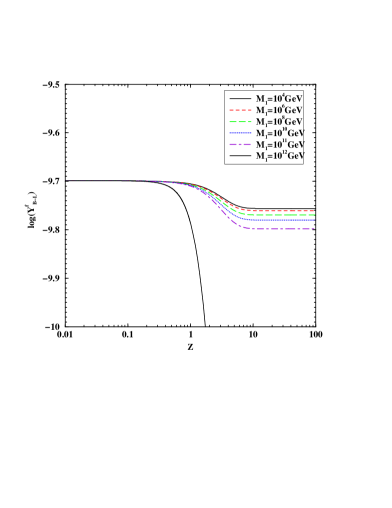
Figure 4.1: The evolution of B-L asymmetry for different values of $M_{1}$ shown against $Z(=M_{1}/T)$ for $\tilde{m}_{1}=10^{-4}$eV and $\eta^{raw}=2.0\times 10^{-10}$

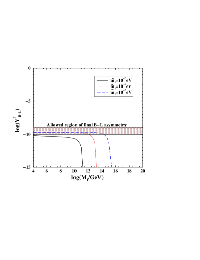
Figure 4.2: The allowed values of $M_{1}$ against the required final asymmetry is shown for $\eta^{raw}=2.0\times 10^{-10}$

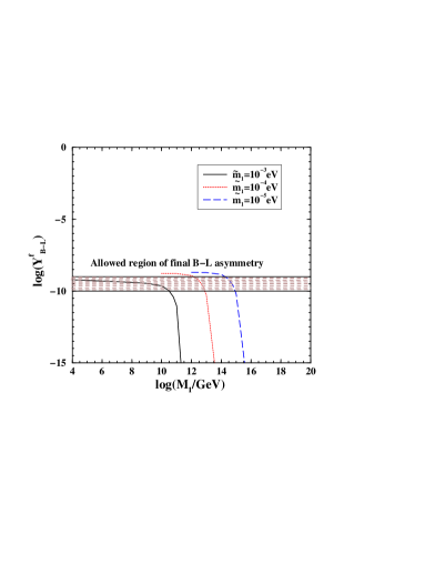
Figure 4.3: The allowed values of $M_{1}$ against the final required asymmetry is shown for $\eta^{raw}=2.0\times 10^{-9}$

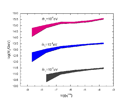
Figure 4.4: The allowed region of $M_{1}$ is shown for different values of $\tilde{m}_{1}$ for large values of $\eta^{\scriptscriptstyle raw}$

The equations (4.8) and (4.9) are solved numerically. The initial $B-L$ asymmetry is the net raw asymmetry produced during the B-L symmetry breaking phase transition by any thermal or non-thermal process. As such we impose the following initial conditions

$$Y^{in}_{N1}=Y^{eq}_{N1}~{}~{}{\mathrm{a}nd}~{}~{}Y^{in}_{B-L}=\eta^{raw}_{B-L}.$$ (4.13)

At temperature $T\geq M_{1}$, wash out effects involving $N_{1}$ are kept under check due to the $\tilde{m}_{1}^{2}$ dependence in (4.11) for small values of $\tilde{m}_{1}$. As a result a given raw asymmetry suffers limited erasure. As the temperature falls below the mass scale of $M_{1}$ the wash out processes become negligible leaving behind a final lepton asymmetry. Fig. 4.1 shows the result of solving the Boltzmann equations for different values of $M_{1}$.

If we demand that the initial raw asymmetry is of the order of $\alpha\times 10^{-10}$, with $\alpha\sim O(1)$, then in order to preserve the final asymmetry of the same order as the initial one it is necessary that the neutrino mass parameter $\tilde{m}_{1}$ should be less than $10^{-3}eV$. This can be seen from fig. 4.2. For $\tilde{m}_{1}=10^{-3}eV$ we can not find any value of $M_{1}$ to preserve the final asymmetry, $\alpha\times 10^{-10}$ in the allowed region. This is because of the large wash out effects as inferred from the equation (4.11). However, for $\tilde{m_{1}}=10^{-4}eV$ we get a lowest threshold on the lightest right handed neutrino of the order $10^{12}GeV$. For any value of $M_{1}\leq 10^{12}GeV$ the final asymmetry lies in the allowed region. This bound increases by two order of magnitude for further one order suppression of the neutrino parameter $\tilde{m}_{1}$. The important point being that $M_{1}=10TeV$ is within the acceptable range.

We now consider the raw asymmetry one order more than the previous case i.e. $\eta^{\scriptscriptstyle raw}_{\scriptscriptstyle B-L}=\alpha\times 10^{-9}$. From fig. 4.3 we see that for $\tilde{m}_{1}=10^{-3}eV$ there is only an upper bound $M_{1}=10^{10.5}GeV$, such that the final asymmetry lies in the allowed region for all smaller values of $M_{1}$. Thus for the case of raw asymmetry an order of magnitude smaller, the upper bound on $M_{1}$ decrease by two orders of magnitude (e.g. compare previous paragraph). However, the choice of smaller values of $\tilde{m}_{1}$ leads to a small window for values of $M_{1}$ for which we end up with the final required asymmetry. In particular for $\tilde{m}_{1}=10^{-4}eV$ the allowed range for $M_{1}$ is ($10^{12}~{}-~{}10^{13})GeV$, while for $\tilde{m}_{1}=10^{-5}eV$ the allowed range shifts to ($10^{14}~{}-~{}10^{15})GeV$. The window effect can be understood as follows. Increasing the value of $M_{1}$ tends to lift the suppression imposed by the $\tilde{m}_{1}^{2}$ dependence of the wash out effects, thus improving efficiency of the latter. However, further increase in $M_{1}$ makes the effects too efficient, erasing the raw asymmetry to insignificant levels.

The windowing effect emerges clearly as we consider the cases of large raw asymmetries. This is shown in fig. 4.4. It is seen that as the raw asymmetry increases the allowed regions become progressively narrower and lie in the range $(10^{10}~{}-~{}10^{15})GeV$. Thus a given raw lepton asymmetry determines a corresponding small range of the heavy Majorana neutrino masses for which we can obtain the final asymmetry of the required order $\alpha\times 10^{-10}$. Again smaller is the effective neutrino mass $\tilde{m}_{1}$ larger is the mean value of the allowed mass of the heavy Majorana neutrino and this is a consequence of normal see-saw.

Finally, in the following, we give an example for non-thermal creation of L-asymmetry in the context of left-right symmetric model.

4.4 Lepton asymmetry in left-right symmetric model

We discuss qualitatively the possibility of lepton asymmetry during the left-right symmetry breaking phase transition [76]. In the following we recapitulate the important aspects of left-right symmetric model for the present purpose and the possible non-thermal mechanism of producing raw lepton asymmetry. This asymmetry which gets converted to baryon asymmetry, can be naturally small if the quartic couplings of the theory are small. Smallness of zero-temperature $CP$ phase is not essential for this mechanism to provide small raw $L$ asymmetry.

4.4.1 Left-Right symmetric model and transient domain walls

The important features of the left-right symmetric model based on the gauge group $SU(2)_{L}\times SU(2)_{R}\times U(1)_{B-L}$ are elucidated in chapter 3. The Higgs potential of the theory naturally entails a vacuum structure wherein at the first stage of symmetry breaking, either one of $\Delta_{L}$ or $\Delta_{R}$ acquires a vacuum expectation value the left-right symmetry, $SU(2)_{L}\leftrightarrow SU(2)_{R}$, breaks. It is required that $\Delta_{R}$ acquires a VEV first, resulting in $SU(2)_{R}\otimes U(1)_{B-L}$ $\rightarrow U(1)_{Y}$. Finally $Q=T^{3}_{L}+T^{3}_{R}+\frac{1}{2}(B-L)$, survives after the bidoublet $\Phi$ and the $\Delta_{L}$ acquire VEVs.

If the left-right symmetry were exact, the first stage of breaking gives rise to stable domain walls [80, 81, 82] interpolating between the L and R-like regions. By L-like we mean regions favored by the observed phenomenology, while in the R-like regions the vacuum expectation value of $\Delta_{R}$ is zero. Unless some non-trivial mechanism prevents this domain structure, the existence of R-like domains would disagree with low energy phenomenology. Furthermore, the domain walls would quickly come to dominate the energy density of the Universe. Thus in this theory a departure from exact symmetry in such a way as to eliminate the R-like regions is essential.

The domain walls formed can be transient if there exists a slight deviation from exact discrete symmetry. As a result the thermal perturbative corrections to the Higgs field free energy will not be symmetric and the domain walls will be unstable. This is possible if the low energy ($\sim 10^{4}$GeV-$10^{9}$GeV) left-right symmetric theory is descended from a Grand Unified Theory (GUT) and the effect is small, suppressed by the GUT mass scale. In the process of cooling the Universe would first pass through the phase transition where this approximate symmetry breaks. The slight difference in free energy between the two types of regions causes a pressure difference across the walls, converting all the R-like regions to L-like regions. Details of this dynamics can be found in ref. [76].

4.4.2 Leptogenesis mechanism

In order to produce adequate lepton asymmetry the following criteria of Skharov’s have to be satisfied  [1]. $C$ and $CP$-violation and finally all the thermal processes have to be out of equilibrium. The first two properties can be realized if there is a $CP$-violating condensate exists in the domain wall. Finally the out-of-equilibrium condition can be realized from the directional motion of the domain walls to R-like regions and thus making all the domains L-like.

We now consider the interaction of neutrinos from the L-R wall, which is moving towards the energetically disfavored phase, the R-like region. The left-handed neutrino, $\nu_{L}$s, are massive in this domain as they couple with their $CP$-conjugate states, where as they are massless in the phase behind the wall as $\langle\Delta_{L}\rangle=0$. This can be seen from the Yukawa coupling

$$\mathcal{L}_{yuk}=f\Delta_{L}\bar{\nu_{L}^{c}}\nu_{L}+h.c.\,$$ (4.14)

and since $\Delta_{L}$ has a wall like profile, the mass of $\Delta_{L}$ is zero behind the wall and is $O(v_{R})$ in front of it.

To get a net lepton-asymmetry one needs the asymmetry between the reflection and transmission coefficients from the wall between $\nu_{L}$ and its $CP$-conjugate state $(\nu^{c}_{L})$. If it favors the transmission of $\nu_{L}$ to the L-like region then the excess of antineutrinos ($\nu^{c}_{L}$) reflected in front of the wall will equilibrate with the $\nu_{L}$ due to helicity flipping scatterings. However the transmitted excess of $\nu_{L}$ remain as it is, since it does not couple with $\nu^{c}_{L}$ behind the wall.

At least two of the Higgs expectation values in L-R model are generically complex, thus providing natural $CP$-violation  [34] permitting all parameters in the Higgs potential to be real. We choose the following profiles for the Higgses

$$\langle\phi\rangle=\begin{pmatrix}k_{1}e^{i\alpha}&0\\ 0&k_{2}\end{pmatrix},~{}~{}\langle\Delta_{L}\rangle=\begin{pmatrix}0&0\\ v_{L}e^{i\theta}&0\end{pmatrix},~{}~{}\langle\Delta_{R}\rangle=\begin{pmatrix}0&0\\ v_{R}&0\end{pmatrix}.$$ (4.15)

In the classical approximation where the wall width is assumed to be large the $CP$ violating phase inside the domain wall becomes position dependent. Under these circumstances a formalism exists [83, 84, 85], wherein the chemical potential $\mu_{\scriptscriptstyle L}$ created for the Lepton number can be computed as a solution of the diffusion equation

$$-D_{\nu}\mu_{\scriptscriptstyle L}^{\prime\prime}-v_{w}\mu_{\scriptscriptstyle L}^{\prime}+\theta(x)\,\Gamma_{\rm hf}\,\mu_{\scriptscriptstyle L}=S(x).$$ (4.16)

Here $D_{\nu}$ is the neutrino diffusion coefficient, $v_{w}$ is the velocity of the wall, taken to be moving in the $+x$ direction, $\Gamma_{\rm hf}$ is the rate of helicity flipping interactions taking place in front of the wall (hence the step function $\theta(x)$), and $S$ is the source term which contains derivatives of the position dependent complex Dirac mass.

After integration of the above equation and using inputs from the numerical solutions we find the raw Lepton asymmetry [76]

$$\eta^{\rm raw}_{\scriptscriptstyle L}\cong 0.01\,v_{w}\frac{1}{g_{*}}\,\frac{M_{1}^{4}}{T^{5}\Delta_{w}}\,$$ (4.17)

where $\eta^{\rm raw}_{\scriptscriptstyle L}$ is the ratio of $n_{L}$ to the entropy density, $s=(2\pi^{2}/45)g_{*}T^{3}$. In the right hand side $M_{1}$ stands for the Majorana neutrino mass, $\Delta_{w}$ is the wall width and $g_{*}$ the effective thermodynamic degrees of freedom at the epoch with temperature $T$. However, the high temperature sphalerons are efficiently converting the $L$ asymmetry into $B-L$ asymmetry. The standard chemical equilibrium calculation  [44] gives $\eta^{\rm raw}_{\scriptscriptstyle B-L}=\frac{79}{51}\eta^{\rm raw}_{\scriptscriptstyle L}$. Using $M_{1}=f\Delta_{\scriptscriptstyle T}$, with $\Delta_{\scriptscriptstyle T}$ is the temperature dependent VEV acquired by the $\Delta_{\scriptscriptstyle R}$ in the phase of interest, and $\Delta_{w}^{-1}=\sqrt{\lambda_{eff}}\Delta_{\scriptscriptstyle T}$ in equation (4.17) we get

$$\eta^{\rm raw}_{\scriptscriptstyle B-L}\cong 10^{-4}v_{w}\left(\frac{\Delta_{\scriptscriptstyle T}}{T}\right)^{5}f^{4}\sqrt{\lambda_{eff}}.$$ (4.18)

Here we have used $g_{*}=110$. Depending on the Majorana Yukawa coupling the raw asymmetry can take a range a values of $O(10^{-4}~{}-~{}10^{-10})$.

4.5 Results and discussions

We have assumed a non-thermal production of raw lepton asymmetry during the $B-L$ breaking phase transition in a generic theory incorporating $B-L$ as a gauge symmetry. If this asymmetry passes without much dilution to be the currently observed baryon asymmetry consistent with WMAP and Big Bang nucleosynthesis, then the effective neutrino mass parameter $\tilde{m}_{1}$ must be less than $10^{-3}eV$. Solution of the relevant Boltzmann equations shows that for $\tilde{m}_{1}=10^{-4}eV$ the mass of lightest right handed neutrino $N_{1}$ has to be smaller than $10^{12}GeV$ and can be as low as $10$ TeV. In a more restrictive scenario where the neutrino Dirac mass matrix is identified with that of the charged leptons it is necessary that $M_{1}>10^{7}GeV$ in order to satisfy $\tilde{m}_{1}<10^{-3}eV$. Therefore in the more restricted scenario all values $M_{1}$, $10^{8}GeV<M_{1}<10^{12}GeV$ can successfully create the required asymmetry. If the Dirac mass scale of neutrinos is less restricted, much lower values of $M_{1}$ are allowed. In particular, a right handed neutrino as low as 10 TeV is admissible.

If the raw asymmetry is large, the numerical solutions show a small window for $M_{1}$ to get the final asymmetry of the required order. The allowed range gets smaller as the raw asymmetry gets larger. This is true for all allowed values of the neutrino mass parameter $\tilde{m}_{1}$.

In summary, if the $B-L$ symmetry is gauged, we start with a clean slate for $B-L$ number and an asymmetry in it can be generated by a non-perturbative mechanism at the scale where it breaks. The presence of heavy right handed neutrinos still permits sufficient asymmetry to be left over in the form of baryons for a large range of values of the $B-L$ breaking scales. While other mechanisms of leptogenesis become unnatural below $10^{7}$ GeV (see for example chapter 1 and chapter 2) this mechanism even tolerates TeV scale. A specific mechanism of this kind is possible in the context of Left-Right symmetric model, presumably embedded in the larger unifying group $SO(10)$. Here we conjecture that upon incorporation of supersymmetry, the qualitative picture will remain unaltered and the present gravitino bound of $10^{9}$ GeV for reheating temperature after inflation can be easily accommodated.

Part-II
Topological Defects Cosmic Strings and Baryogenesis via Leptogenesis

Chapter 5 Soliton fermion systems in Quantum Field Theory

5.1 Introduction

“Solitary waves” and “solitons” emerge as the non perturbative solutions of non-linear wave equations in classical field theory. These are non-dispersive localized packets of energy moving uniformly in space. Although they have many common features, the former class of solutions do not keep their shape intact during a collision among themselves, whereas the latter do in the asymptotic time domain. Thus the latter class of solutions is a special subset of the former class of solutions, but the converse is not necessarily true. Having differentiated solitons from solitary waves, we should mention (without embarking into details) that the distinction between them in field theory is completely blurred. So here onwards, what merely called as “solitary wave”, we call it “soliton” as it is more crisp and appealing. A prototype example in field theory is the well known massive Thirring model where the solution is exactly solitonic.

It was believed that elementary particles in nature can be thought of as localized packets of energy, the prime among such theories is the famous Skyrme model. But till date no satisfactory formalism has been developed to view elementary particles as solitons as the present effective theory takes particles as point like, nor is there any experimental evidence at latest attainable energies to prove that particles have indeed extended features. We bypass this issue here but concentrate on defects occurring in gauge theories. Of course field theories describing elementary particles are quantum theories, whereas solitons are solutions of classical field theories. Although it is a classical solution, the quantization of bosonic fluctuation in the background of this non trivial vacuum, the so called “semiclassical treatment”, leads to a finite correction [86].

A topological solution can be obtained as a solution of a differential equation with a difficulty that the boundary values are known only at infinity. In the context of field theories a prototype example is the ‘kink’, which emerge as the solution of $\phi^{4}$-theory in 1+1 dimensions. For demonstration purpose, in section 5.2 we consider a toy model in 1+1 dimensions.

A more curious phenomenon happens in Quantum Field Theory (QFT) when a fermion interacts with a kink. This was first pointed out by Jackiw and Rebbi [47] in 1976. It was shown that the resulting fermion number becomes fractionalized. Although it is surprising, the consequences of this phenomena have already been studied extensively in literature in the context of condensed matter systems, polyacetylene being the standard example [87, 88, 89, 90], and in high energy physics, cosmic string being the example [50, 91].

5.2 Solitary waves in 1+1 dimensions

Soliton or solitary wave is a static, localized and finite energy solution of non-linear wave equation in classical field theory. For the present purpose we consider only bosonic fields $\phi(x,t)$ in one space and one time dimensions. The dynamics of the fields is governed by the Lagrangian

$$\mathcal{L}=\frac{1}{2}\partial_{\mu}\phi\partial^{\mu}\phi-V(\phi)\\ ,$$ (5.1)

where $V(\phi)$ is the required potential. In $\lambda\phi^{4}$-theory it is given by

$$V(\phi)=\frac{\lambda}{2}\left(\phi^{2}-\frac{\mu^{2}}{\lambda}\right)^{2}.$$ (5.2)

The Hamiltonian corresponding to the Lagrangian (5.1) is

$$\mathcal{H}=\frac{1}{2}\partial_{\mu}\phi\partial^{\mu}\phi+V(\phi).$$ (5.3)

In order to get solitonic solutions we demand that $\phi$ is independent of time. Thus the equation of motion will be

$$\frac{\partial^{2}\phi}{\partial x^{2}}=\frac{\partial V(\phi)}{\partial\phi}.$$ (5.4)

Again the finiteness of the energy requires that the energy functional

$$E[\phi]=\int_{-\infty}^{+\infty}dx\left[\frac{1}{2}\left(\frac{d\phi}{dx}\right)^{2}+V(\phi)\right]<\infty.$$ (5.5)

If the absolute minima of $V(\phi)$, which are also its zeros, occur at n points i.e

$$V(\phi)=0\hskip 28.45274ptfor\hskip 14.22636pt\phi=g^{i},i=1,2\cdots n$$ (5.6)

then the energy functional $E[\phi]$ can be minimized when the field $\phi(x,t)$ is constant in space-time and takes any one of these values. That is $E[\phi]=0$ if and only if $\phi(x,t)=g^{i}$. Further to make $E[\phi]$ finite at spatial infinity $(x\rightarrow\pm\infty)$, it requires that $V(\phi)=0$ at $x\rightarrow\pm\infty$, which is the absolute minimum of $V(\phi)$. In addition to that $\frac{d\phi}{dx}=0$. This implies that $\phi$=constant.

We now solve Eqn.(5.4). One of the easiest way to solve this equation is that, if we replace

$$\phi \leftrightarrow y$$

$$x \leftrightarrow t$$

$$V(\phi) \leftrightarrow -V(\phi)$$

in equation (5.4) then it will resemble with newtons second law of motion of a particle of unit mass moving in a negative potential. The solution $\phi(x)$ represents this particle’s motion of this analogue particle. So the total energy of this motion is conserved as x, the time, varies and is given by

$$W=\frac{1}{2}\left(\frac{d\phi}{dx}\right)^{2}-V(\phi).$$ (5.7)

Note that this energy is different from the energy of the soliton. Now using the above boundary conditions (used for soliton), we have $W=0$. This gives rise to

$$\int_{0}^{x}dx=\pm\int_{\phi(0)}^{\phi(x)}\frac{d\phi}{\sqrt{2V(\phi)}}.$$ (5.8)

Solving this equation for the particular potential defined in Eqn.(5.2) we get

$$\phi_{\pm}(x)=\pm\frac{\mu}{\sqrt{\lambda}}\tanh(\mu x).$$ (5.9)

The solution corresponding to $\phi_{+}(x)$ is called ‘kink’ and that of $\phi_{-}(x)$ is called ‘antikink’. Note that the coupling constant $\lambda$ appear in the denominator of the above Eqn.(5.9). If $\lambda\rightarrow 0$ then the corresponding solution $\phi\rightarrow\infty$. Thus the phenomenon is completely non-perturbative one. The energy corresponding to these solutions is given by

$$E=\int_{-\infty}^{+\infty}\epsilon dx,$$ (5.10)

where

$$\epsilon=\frac{\mu^{4}}{\lambda}{\mathrm{s}ech}^{4}(\mu x).$$ (5.11)

Sometimes this energy is called classical ‘kink mass’ $M_{cl}=E=\frac{4\mu^{3}}{3\lambda}$. At this point it is worth to point out the symmetric properties between kink and antikink. It is clear from equation (5.9) that

$$\phi_{+}(x) = -\phi_{-}(x)$$ (5.12)

$$= \phi_{-}(-x).$$

Thus a kink starts its motion from a trivial vacuum $\phi=-\frac{\mu}{\sqrt{\lambda}}$ at $x\rightarrow-\infty$ to reach other trivial vacuum $\phi=\frac{\mu}{\sqrt{\lambda}}$ at $x\rightarrow+\infty$ through zero. Although these are extended objects still its energy is concentrated within narrow region of space of $O(1/\mu)$. So these solutions is expected to behave as particles in high energy physics. Fortunately these solutions admit a Lorentz boost with a definite velocity ($v$). For example, the energy of the soliton transforms as

$$E\rightarrow E^{{}^{\prime}}=\frac{E}{\sqrt{1-v^{2}}}.$$ (5.13)

It is worth to point out that kink is merely a solitary wave and not a soliton. That means they do not survive collisions. Since in our current discussion (i.e. in context of $\phi^{4}$-theory) there is only a pair of kink and antikink solution exist, so it is difficult to check their shape retaining property in a collision. Of course, a numerical calculation is needed to check it. But it is beyond the scope of this manuscript.

5.3 Topological charge

Often we need to distinguish the topological solutions of a system of equations. So we define a ‘topological index’, which is conserved in time. It is very similar to ‘quantum number’ in QFT, but its origin is completely different. Now we will illustrate it in context of $\lambda\phi^{4}$ -theory. The potential has two degenerate minima, at $\phi=\pm\frac{\mu}{\sqrt{\lambda}}$. Consequently solutions of this system, whether static or time dependent, fall into four topological sectors. These are characterized by the pair of indices $(-\frac{\mu}{\sqrt{\lambda}},\frac{\mu}{\sqrt{\lambda}})$, $(\frac{\mu}{\sqrt{\lambda}},-\frac{\mu}{\sqrt{\lambda}})$, $(-\frac{\mu}{\sqrt{\lambda}},-\frac{\mu}{\sqrt{\lambda}})$, $(\frac{\mu}{\sqrt{\lambda}},\frac{\mu}{\sqrt{\lambda}})$ respectively. Where the quantities inside the parenthesis represents the value of $\phi_{\pm}(x)$ at their spatial infinity. Now we choose a particular sector $(-\frac{\mu}{\sqrt{\lambda}},-\frac{\mu}{\sqrt{\lambda}})$, which is nothing but the value of kink at $x\rightarrow-\infty$ and antikink at $x\rightarrow\infty$. Even though we may not be able to calculate easily what happens after they collide, but we can be sure that the resulting field configuration will lie in the $(-\frac{\mu}{\sqrt{\lambda}},-\frac{\mu}{\sqrt{\lambda}})$ sector. At this juncture it is worth to designate such sectors by a definite quantity called ‘topological charge’, defined by

$$Q=\frac{\sqrt{\lambda}}{\mu}\left[\phi(x=+\infty)-\phi(x=-\infty)\right],$$ (5.14)

associated with a conserved current

$$k^{\alpha}=\frac{\sqrt{\lambda}}{\mu}\epsilon^{\alpha\beta}\partial_{\beta}\phi\,$$ (5.15)

where $\alpha$, $\beta$= 0, 1. From equation (5.15) we get the topological charge

$$Q=\int_{-\infty}^{+\infty}k_{0}dx.$$ (5.16)

Thus we need both $\phi(\infty)$ and $\phi(-\infty)$ to identify a topological sector. If $Q=0$, then the object is a non topological object. Thus topological charges are nothing but the boundary conditions of the problem in contrast to usual Noether charge in QFT which comes from the continuous symmetry associated with the theory.

5.4 Fractional fermion charge in QFT

The phenomenon of fractional charge was first discovered by Jackiw and Rebbi [47] in their pioneering work in 1976. We begin by reviewing their work. Note that the charges we are talking about are not the wellknown and widely accepted fractional charge of quarks. But it is the charge which appear as the eigen value of number operator in the QFT. For our illustration purpose, we consider the 1+1-dimensional theory.

As an extension of equation (5.1) to include fermion field $\psi$, the additional terms are given by the Lagrangian

$$\mathcal{L}_{fermion}=\bar{\psi}\left(i\gamma^{\nu}\partial_{\nu}-g\phi(x,t)\right)\psi.$$ (5.17)

For the potential defined in equation (5.2), the trivial vacuua are $\phi=\pm\frac{\mu}{\sqrt{\lambda}}$. It is well known that the presence of two degenerate classical solutions indicate spontaneous breaking of the $\phi\rightarrow-\phi$ symmetry of the Lagrangian (5.1). Around each of these classical vacuua a whole tower of Fock states can be built and hence to be called vacuum sectors. In addition to that the system has also two other static solutions. Those are the solitonic solutions, the so called kink and its reflected partner the anti-kink, given respectively by

$$\phi_{s}=\pm\frac{\mu}{\sqrt{\lambda}}\tanh(\mu x).$$ (5.18)

As per the general theory of semi classical quantization of quantum fields, one can build two other separate towers of states, one around each of these solitonic solutions. In short, we have four sectors of states for this interacting system: two are the vacuum sectors built around $\phi=\pm\frac{\mu}{\sqrt{\lambda}}$ and others two are the soliton sectors $\pm(\mu/\sqrt{\lambda})\tanh(\mu x)$.

5.4.1 The vacuum sector

In the vacuum sector, $\phi=+\frac{\mu}{\sqrt{\lambda}}$, the Lagrangian for the fermion field $\psi$ is given by

$$\mathcal{L}=\bar{\psi}\left(i\gamma^{\nu}\partial_{\nu}-m_{F}\right)\psi\\ ,$$ (5.19)

where $m_{F}=g(\mu/\sqrt{\lambda})$ is the mass of the fermion and $\nu$ stands for 0,1. Since we have only one space dimension, we use the representation of the Dirac matrices as $\gamma^{1}=\beta\alpha=i\sigma^{3}$ and $\gamma^{0}=\beta=\sigma^{1}$. Let us denote by $u_{k}(x)$ and $v_{k}(x)$ the positive and negative energy spinorial solutions of the Dirac equations

$$(-i\alpha\partial_{x}+\beta m_{F})u_{k}(x) = E_{k}u_{k}(x)$$ (5.20)

$$(-i\alpha\partial_{x}+\beta m_{F})v_{k}(x) = -E_{k}v_{k}(x),$$ (5.21)

where $E_{k}=+\sqrt{k^{2}+m_{F}^{2}}$ and spinor indices have been suppressed. The Dirac field can be expanded in terms of these solutions and the destruction operators $b_{k}$ and $d_{k}$, obeying the usual anticommutation rules, as

$$\psi(x,t)=\sum_{k}[b_{k}u_{k}e^{-iE_{k}t}+d_{k}^{\dagger}v_{k}e^{iE_{k}t}].$$ (5.22)

The vacuum state in the $\phi=(+\mu/\sqrt{\lambda})$ sector is given by the conditions

$$b_{k}|0\rangle=d_{k}|0\rangle=0$$ (5.23)

with all the bosonic oscillators being in the ground state.

Note that the third Pauli matrix $\sigma^{3}$ acts as the charge conjugation matrix. It anticommutes with the Dirac Hamiltonian in Eq. (5.21) and generates for every positive energy solution $u_{k}(x)$ of energy $E_{k}$ the corresponding negative energy solution $v_{k}(x)$ of energy $-E_{k}$, i.e.

$$\sigma^{3}u_{k}(x)=v_{k}(x).$$ (5.24)

Hence all modes of the expansion (5.22) come in pairs with equal positive and negative energies. There are no zero energy solutions for $\psi$ in the vacuum sector that allowed by the Dirac equations (5.20) and (5.21).

Finally we consider the number density operator

$$\rho(x,t)=\frac{1}{2}\left[\psi^{\dagger}(x,t),\psi(x,t)\right].$$ (5.25)

The form of $\rho$ is designed so as to be odd under charge conjugation. Inserting the mode expansion (5.22) and using the orthonormality conditions of the Dirac spinors, the total charge becomes

$$Q = \int dx\rho(x,t)$$ (5.26)

$$= \frac{1}{2}\sum_{k}\left([b^{\dagger}_{k},b_{k}]+[d_{k},d^{\dagger}_{k}]\right)$$

$$= \sum_{k}\left([b^{\dagger}_{k}b_{k}-1/2]-[d^{\dagger}_{k}d_{k}-1/2]\right)$$

$$= \sum_{k}\left(b^{\dagger}_{k}b_{k}-d^{\dagger}_{k}d_{k}\right).$$

Notice that the half-integers cancel term by term because of the existence of paired positive and negative energy modes. Hence the familiar result in the vacuum sector that the charge operator has only integer eigenvalues.

5.4.2 The soliton Sector

In this section, we repeat the same procedure as we did in the trivial vacuum sector. We replace the $\phi$ by its solitonic value $\phi_{s}$ from Eq. (5.18). The corresponding Dirac equation becomes

$$\left(-i\alpha\partial_{x}+\beta m_{F}\tanh(\mu x)\right)\psi(x)=E\psi(x).$$ (5.27)

This equation has a set of positive energy solutions $\psi_{k}(x)$ associated with energy $E_{k}$. However, the charge conjugation matrix $\sigma^{3}$ again anticommutes with the Dirac Hamiltonian, $C^{-1}HC=-H$. Therefore, for every positive energy solution $\psi_{k}(x)$ there is a negative energy solution $\tilde{\psi_{k}}(x)$ with energy $-E_{k}$.

For the two components $\psi_{1,2}$ of the Dirac spinor, equation (5.27) yields the coupled equations

$$\left(-\partial_{x}+m_{F}\tanh(\mu x)\right)\psi_{2} = E\psi_{1}$$ (5.28)

$$\left(\partial_{x}+m_{F}\tanh(\mu x)\right)\psi_{1} = E\psi_{2}.$$ (5.29)

Solving these coupled equations we get an unpaired zero-energy solution

$$\psi_{0}=\begin{pmatrix}Nexp\left(-m_{F}\int_{0}^{x}dx^{\prime}\tanh(\mu x^{\prime})\right)\\ 0\end{pmatrix}.$$ (5.30)

In contrast to the normal vacuum, in the soliton sector we have a zero energy solution (5.30). This is because of the soliton function $(\mu/\sqrt{\lambda})\tanh(\mu x)$ which forms the background potential for the Dirac spinor tends to opposing limits $\pm(\mu/\sqrt{\lambda})$ as $x\rightarrow\pm\infty$. In infinite spatial volume this solution has no partner. It is self charge conjugate i.e. $\sigma^{3}\psi_{0}=\psi_{0}$. The mode expansion of the Dirac field operator now becomes

$$\psi(x,t)=\sum_{k\neq 0}\left[b_{k}\eta_{k}(x)e^{-iE_{k}t}+d^{\dagger}_{k}\tilde{\eta_{k}}(x)e^{iE_{k}t}\right]+a\psi_{0}(x)$$ (5.31)

where ‘a’ is the destruction operator for the zero mode $\psi_{0}$.

Unlike the vacuum sector built around $(\mu/\sqrt{\lambda})$ which had a unique ground state, in the solitonic sector there exists two degenerate ground states because of the existence of a zero energy solution of $\psi$. They are $|sol\rangle_{-}$, being the unfilled state, and $|sol\rangle_{+}$, being the filled state, obeying

$$a_{k}|sol\rangle_{-}=b_{k}|sol\rangle_{-}=d_{k}|sol\rangle_{-}=0$$ (5.32)

and

$$|sol\rangle_{+} = a^{\dagger}|sol\rangle_{-}$$

$$a|sol\rangle_{+} = |sol\rangle_{-}.$$ (5.33)

These are the two basic quantum soliton states of this system. They are energetically degenerate, but are distinguishable by their charge

$$Q = \frac{1}{2}\int dx\left[\psi^{\dagger}(x,t),\psi(x,t)\right]$$ (5.34)

$$= \frac{1}{2}\sum_{k}\left([b^{\dagger}_{k},b_{k}]+[d_{k},d^{\dagger}_{k}]\right)+(1/2)[a^{\dagger},a]$$

$$= \sum_{k}\left((b^{\dagger}_{k}b_{k}-1/2)-(d^{\dagger}_{k}d_{k}-1/2)\right)+(a^{\dagger}a-1/2)$$

$$= \sum_{k}\left(b^{\dagger}_{k}b_{k}-d^{\dagger}_{k}d_{k}\right)+(a^{\dagger}a-1/2)$$

Notice that the piece (-1/2) coming from the zero mode commutator remains uncanceled because it does not have a charge conjugate partner. Thus it is obvious that the total charge (the number operator) Q has half integral eigen values. The two degenerate soliton states have eigen values $\pm 1/2$ respectively for the total number operator Q:

$$Q|sol\rangle_{-} = -(1/2)|sol\rangle_{-}$$

$$Q|sol\rangle_{+} = (1/2)|sol\rangle_{+}$$ (5.35)

Thus the solitonic states are superselected from the normal vacuum due to the unavailability of fractional states in the translational invariant vacuum. Note that the fractionalization of the fermion number in the background of a nontrivial vacuum is one of the manifestation of Dirac negative energy sea.

5.5 Implication of fermion zero modes and superselection rules

By the name ‘superselection’ we mean that there are certain restrictions on nature and scope of possible measurements. It is shown that [92] there exist superselection rules for spinor fields which can be proved in context of the assignment of parity to the quantum mechanical states of a system.

The usual assumption in quantum mechanics is that it is possible to carry out a complete set of measurements; the result of which determines the state of any vector completely except for the usual phase factor. If there exist sectors $A$, $B$, $C$, etc. in the Hilbert space such that vectors in each subspace can be independently rescaled by phases, such sectors must be understood to be completely independent, and superposition of states from such unrelated sectors should be forbidden. Specifically, let state vectors $\Psi_{A}$, $\Psi_{B}$,$\Psi_{C}$ etc. belong to such independent sectors, so that it is assumed that no physical measurements distinguish between the state

$$\Psi_{A}+\Psi_{B}+\Psi_{C}+\ldots$$ (5.36)

and

$$e^{i\alpha}\Psi_{A}+e^{i\beta}\Psi_{B}+e^{i\gamma}\Psi_{C}+\ldots$$ (5.37)

where $\alpha$, $\beta$, $\gamma$, $\ldots$ are arbitrary phases. Then the expectation value of any operator possessing matrix elements connecting subspaces $A$ and $B$, or $A$ and $C$, etc. must be completely undefined. Hence such an operator will not correspond to a measurable quantity.

It is customary to say that a selection rule operates between subspace of the total Hilbert space if the state vectors of each subspace remain orthogonal to all state vectors of other subspaces as long as the system is isolated. There is, for instance, a selection rule which prevents any state of an isolated system from changing its total linear momentum. Similarly, the state vectors of the subspace containing all states with total angular momentum J will remain, in a closed systems, orthogonal to all states with any other total angular momentum. So we shall say that a superselection rule operates between subspaces if there does not exist any selection rule between them and if, in addition to this, there are no measurable quantities with finite matrix elements between their state vectors. For example if we superpose states of integral spin (bosonic) with half integral spin (fermionic) then the probability of finding of each states are equal and 1/2 each. So it is impossible to compare directly a spin half particle with a spin one particle. It is conjectured that [92] superselection rule not only work between the states of different intrinsic parity but also it works between the states of different total charge. For instance if we construct a state, by superposing the states $|1/2\rangle$ and $|1\rangle$, as

$$\psi_{s}=\frac{1}{2}[|1/2\rangle+|1\rangle]$$ (5.38)

then it is expected that under $P^{4}$ operation it will come back to it’s original state up to a phase. To verify this we can assign a parity $\pm 1$ to a Dirac neutrino and $\pm i$ to a Majorana neutrino in the trivial vacuum sector. But in the vortex sector the corresponding state is doubly degenerate and thus the parity assignment is half of their trivial vacuum values. Now the $P^{4}$ operation on (5.38) for a Majorana neutrino will give

$$P^{4}\psi_{s}=\frac{1}{2}[-|1/2\rangle+|1\rangle].$$ (5.39)

This state is another state orthogonal to (5.38) and hence implies the impossibility of superposition of such states. We discuss more about it in context of the decay of cosmic strings in chapter 6.

Chapter 6 Metastable topological defects and fermion zero modes

6.1 Introduction

In the process of cooling down from the highest possible energy scale till the present epoch, early Universe has been passed through several phase transitions. A phase transition occurs through the spontaneous breaking of a larger gauge symmetry group $G$ to any of its subgroup $H$. If the corresponding vacuum manifold ${\cal M}=G/H$ is non trivial then the topological defects are formed. Depending on the geometry of the manifold the possible defects are domain walls, cosmic strings, monopoles and textures. Domain walls form if ${\cal M}$ has disconnected components, strings can form if ${\cal M}$ has unshrinkable loops and monopoles form when ${\cal M}$ contains unshrinkable surfaces. The relevant properties of the manifold ${\cal M}$ are most conveniently studied using homotopy theory; the $n^{th}$ homotopy group $\pi_{n}({\cal M})$ classifies qualitatively distinct mappings from the n-dimensional sphere $S^{n}$ into the manifold ${\cal M}$. If $\pi_{0}({\cal M})\neq I$ then the formed defects are called domain walls. On the other hand, if $\pi_{1}({\cal M})\neq I$ then cosmic strings are formed and if $\pi_{2}({\cal M})\neq I$ then monopoles are formed. These are extended objects, cosmic strings being 1+1-dimensional, domain walls the 2+1-dimensional and finally monopoles the 3+1-dimensional but not point like.

The topological defects emerge as the solitonic solutions of non linear wave equations in gauge theories. Therefore, in the asymptotic time domain these objects are very stable and keep their original configurations in tact. However, they can be unwound by overcoming finite energy barriers. The dynamics of these objects may have several consequences that may link to the physics of early Universe with the recent cosmology. In particular, we discuss baryogenesis via leptogenesis from the decay products of cosmic strings in chapter 7.

6.2 Metastable topological defects

If there are several stages of symmetry breaking, the topological stability of these extended objects depend on the structure of the vacuum manifold at every stage. Under certain conditions defects stable at the first stage of symmetry breaking are rendered unstable at lower temperatures. Likewise objects that seem to enjoy topological stability in the low energy effective theory are actually unstable in the complete description of the theory. The instability however tends to energetically exorbitant thus rendering the object metastable [93].

There are several reasons that may stabilize objects that are unstable on topological grounds. For instance superconducting strings lead to small loops called vortons, stabilized by the electric current flowing through them. Here we consider the occurrence of fermionic zero-energy modes. As a rule of thumb, if the number of trapped zero-energy modes is $n$, the ground state of the defect carries fermion number $n/2$. Thus if $n$ is odd one obtains curious occurrence of fractionalization of fermion number, proven to be integer in translation invariant field theory. In general there are several internal charges the fermions may carry and the fractionalization rule affects all of them. It has been observed by several authors [94, 95, 96] that the unavailability of final states of matching charge should forbid the decay of such objects in isolation.

Here we consider the sequential breakdown of the gauge group $G\rightarrow H_{1}\rightarrow H_{2}$. If the vacuum manifold ${\cal M}=G/H_{1}$ is non-trivial then topological defects are formed. However, these defects in their corresponding low energy theories loss their stability after the breaking of second phase of symmetry if the manifold $G/H_{2}$ is simply connected and thus making the defect metastable. As an example we study the metastable cosmic strings in sec. 6.2.1.

6.2.1 Metastable cosmic strings and fermion zero modes

Here we construct two examples in which the cosmic strings of a low energy theory are metastable due to the embedding of the low energy symmetry group in a larger symmetry group at higher energy. Examples of this kind were considered in [93]. Borrowing the strategies for bosonic sector from there, we include appropriate fermionic content to ensure the zero-modes.

A. Dirac fermions

Consider first a model with two stages of symmetry breaking similar to [93], but with local $SU(2)$ gauge invariance. The two scalars $\vec{\Sigma}$ and $\sigma$ are respectively real triplet and complex doublet. The Lagrangian is taken to be

$$\mathcal{L} = -\frac{1}{4}F^{\mu\nu a}F^{a}_{\mu\nu}+\frac{1}{2}D_{\mu}{\vec{\Sigma}}\cdot D^{\mu}\vec{\Sigma}+D_{\mu}\sigma^{\dagger}D^{\mu}\sigma$$ (6.1)

$$- \lambda_{1}(\vec{\Sigma}\cdot\vec{\Sigma}-\eta_{1}^{2})^{2}-\lambda_{2}(\sigma^{\dagger}\sigma-\eta_{2}^{2})^{2}$$

$$+ \lambda_{12}\eta_{1}\vec{\Sigma}\cdot\sigma^{\dagger}{\vec{\tau}}\sigma$$

where isovector notation is used and $\tau$ are the Pauli matrices. It is assumed that $\eta_{1}\gg\eta_{2}$ and that the coupling $\lambda_{12}>0$ satisfies $\lambda_{12}\eta_{1}^{2}\ll$ $\lambda_{2}\eta_{2}^{2}$

The vacuum expectation value (VEV) $\vec{\Sigma}=(0\ 0\ \eta_{1})^{T}$ breaks the $SU(2)$ to the $U(1)$ generated by $\exp(i\tau^{3}\alpha/2)$. The effective theory of the $\sigma$ can be rewritten as the theory of two complex scalar $\sigma_{u}$ and $\sigma_{d}$ for the up and the down components respectively. The potential of the effective theory favors the minimum

$$\sigma_{u}=\eta_{2},\qquad\sigma_{d}=0$$ (6.2)

In the effective theory $\sigma_{u}$ enjoys a $U(1)$ invariance $\sigma_{u}\rightarrow e^{i\alpha}\sigma_{u}$ which is broken by the above VEV to $\mathbb{Z}\equiv\{e^{2n\pi i}\}$, $n=1,2,\ldots$. This makes possible vortex solutions with an ansatz in the lowest winding number sector

$$\sigma_{u}(r,\phi)=\eta_{2}f(r)e^{-i\phi}$$ (6.3)

where $r,\phi$ are planar coordinates with vortex aligned along the $z$ axis. The vortex configuration is a local minimum, however it can decay by spontaneous formation of a monopole-antimonopole pair [93]. These monopoles are permitted by the first breaking $SO(3)\rightarrow SO(2)$ in the $\Sigma$ sector. Paraphrasing the discussion of  [93], we have $SU(2)\rightarrow$$U(1)\rightarrow\mathbb{Z}$. The vortices are stable in the low energy theory because $\pi_{1}(U(1)/\mathbb{Z})$ is nontrivial. But in the $SU(2)$, the $\mathbb{Z}$ lifts to $\{e^{4n\pi i\tau^{3}/2}\}=I$ making it possible to unwind the vortex by crossing an energy barrier.

Consider now the introduction of a doublet of fermion species $\psi_{L}^{T}\equiv(N_{L},E_{L})$ assumed to be left handed and a singlet right handed species $N_{R}$. The Yukawa coupling of these to the $\sigma_{u}$ is given by $h{\overline{N_{R}}}\sigma^{\dagger}\psi_{L}$, which in the vortex sector reads

$$\mathcal{L}_{\sigma-\psi}\sim h\eta_{2}f(r)(e^{-i\phi}{\overline{N_{R}}}N_{L}+h.c.)$$ (6.4)

The lowest energy bound states resulting from this coupling are characterized by a topological index, [51] $\mathcal{I}\equiv n_{L}-n_{R}$ where $n_{L}$ and $n_{R}$ are the zero modes of the left handed and the right handed fermions respectively. This index can be computed using the formula [51, 97]

$$\mathcal{I}=\frac{1}{2\pi i}(\ln\textrm{det}M)|^{2\pi}_{\phi=0}$$ (6.5)

where $M$ is the position dependent effective mass matrix for the fermions. In the present case this gives rise to a single zero-energy mode for the fermions of species $N$. According to well known reasoning [47] to be recapitulated below, this requires the assignment of either of the values $\pm 1/2$ to the fermion number of this configuration.

B. Majorana fermions

The example above can be extended to the case where the $N_{R}$ is a Majorana fermion. Being a singlet $N_{R}$ admits a mass term $M_{\scriptstyle M}{\overline{N_{R}^{\scriptstyle C}}}N_{R}$, $M_{\scriptstyle M}$ signifying Majorana mass. This could also be a spontaneously generated mass due to the presence of a neutral scalar $\chi$ with coupling terms $h_{\scriptstyle M}\chi{\overline{N_{R}^{\scriptstyle C}}}N_{R}+h.c.$. If this $\chi$ acquires a VEV at energies higher than the $\Sigma$, the $N_{R}$ particles possess a Majorana mass and fermion number is not a conserved observable.

Finally we present the case where Majorana mass is spontaneously generated at the same scale at which the vortex forms. Consider a theory with local $SU(3)$ symmetry broken to $U(1)$ by two scalars, $\Phi$ an octet acquiring a VEV $\eta_{1}\lambda_{3}$ ($\lambda_{3}$ here being the third Gell-Mann matrix) and $\phi$, a ${\bar{3}}$, acquiring the VEV $\langle\phi^{k}\rangle=\eta_{2}\delta^{k2}$, with $\eta_{2}\ll\eta_{1}$. Thus

$$SU(3){\buildrel 8\over{\longrightarrow}}U(1)_{3}\otimes U(1)_{8}{\buildrel\overline{3}\over{\longrightarrow}}U(1)_{+}$$ (6.6)

Here $U(1)_{3}$ and $U(1)_{8}$ are generated by $\lambda_{3}$ and $\lambda_{8}$ respectively, and $U(1)_{+}$ is generated by $(\sqrt{3}\lambda_{8}+\lambda_{3})/2$ and likewise $U(1)_{-}$ to be used below. It can be checked that this pattern of VEVs can be generically obtained from the quartic scalar potential of the above Higgses. The effective theory at the second breaking $U(1)_{-}\rightarrow\mathbb{Z}$ gives rise to cosmic strings. However the $\mathbb{Z}$ lifts to identity in the $SU(3)$ so that the string can break with the formation of monopole-antimonopole pair.

Now add a multiplet of left-handed fermions belonging to $\overline{15}$. Its mass terms arise from the following coupling to the $\overline{3}$

$$\mathcal{L}_{\textrm{Majorana}}=h_{\scriptstyle M}\overline{\psi^{\scriptstyle C}}^{\{ij\}}_{k}\psi^{\{lm\}}_{n}\phi^{r}(\epsilon_{ilr}\delta^{n}_{j}\delta^{k}_{m})$$ (6.7)

The indices symmetric under exchange have been indicated by curly brackets. No mass terms result from the $8$ because it cannot provide a singlet from tensor product with $\overline{15}\otimes\overline{15}$ [19]. After substituting the $\phi$ VEV a systematic enumeration shows that all but the two components $\psi^{\{22\}}_{1}$ and $\psi^{\{22\}}_{3}$ acquire Majorana masses at the second stage of the breaking. Specifically we find the Majorana mass matrix to be indeed rank $13$. Thus, using either of the results [50] or [97] i.e.,  eq.(6.5) we can see that there will be $13$ zero modes present in the lowest winding sector of the cosmic string. Thus the induced fermion number differs from that of the vacuum by half-integer as required.

C. Final state zero-modes

The stability argument being advanced is in jeopardy if the final state after rupture of the topological object also possesses half-integral fermionic charge. To see that this is not the case it is necessary to study the zero-modes on the two semi-infinite strings shown in fig. 6.1. Generically we expect each of the halves to support the same number of zero-modes, making the total fermion number of the putative final state integer valued, as required for the validity of our argument.

Figure 6.1: Schematic configuration of isospin vectors after the rupture of a string. Internal orientations are mapped to external space. They are shown just outside the core of the two resulting pieces and on the mid-plane symmetrically separating the two.

Consider the ansatz for the lower piece ($l$) with origin at the corresponding monopole and coordinates $(r_{l},\theta_{l},\phi)$. For the domain $z<0$ let the ansatz for the field $\sigma$ be

$$U_{l}^{\infty}(\theta_{l},\phi)\begin{pmatrix}0\\ \eta_{2}\end{pmatrix}f_{l}(r_{l})\equiv\exp\{\frac{i}{2}\theta_{l}{\vec{\tau}}\cdot\hat{\phi}\}\begin{pmatrix}0\\ \eta_{2}\end{pmatrix}f_{l}(r_{l})$$ (6.8)

so that $\langle\sigma\rangle$ has the behavior

$$\langle\sigma\rangle=\left\{\begin{array}[]{lr}\begin{pmatrix}0\\ \eta_{2}\end{pmatrix}f_{l}(r_{l})&\textrm{for}\ \theta_{l}\approx 0\\ &\\ \begin{pmatrix}\eta_{2}e^{-i\phi}\\ 0\end{pmatrix}f_{l}(r_{l})&\textrm{for}\ \theta_{l}\approx\pi\end{array}\right.$$

which agrees with the ansatz (6.3) for the cosmic string at the South pole. Likewise for the domain $z>0$, i.e. the upper piece ($u$), we choose

$$U_{u}^{\infty}(\theta_{u},\phi)=\exp\{\frac{i}{2}(\pi-\theta_{u}){\vec{\tau}}\cdot\hat{\phi}\}$$ (6.9)

resulting in the behavior

$$\langle\sigma\rangle=\left\{\begin{array}[]{lr}\begin{pmatrix}\eta_{2}e^{-i\phi}\\ 0\end{pmatrix}f_{u}(r_{u})&\textrm{for}\ \theta_{u}\approx 0\\ &\\ \begin{pmatrix}0\\ \eta_{2}\end{pmatrix}f_{u}(r_{u})&\textrm{for}\ \theta_{u}\approx\pi\end{array}\right.$$

thus matching correctly with the cosmic string at the North pole. The ansatz for the heavier scalar $\Sigma$ needs to be appropriately set up, $U^{\infty}{\vec{\Sigma}}\cdot{\vec{\tau}}{U^{\infty}}^{\dagger}$ in both $l$ and $u$ domains. This scalar however does not contribute to fermion mass matrix.

The two maps match at the mid-plane where $\theta_{l}=\pi-\theta_{u}$ and $\sigma_{u}\sim e^{-i\phi}$ at $\theta_{l}=\theta_{u}=\pi/2$ so that we have ensured that the combined map is within the same homotopy class as the string we began with. Finally, as the two pieces move far away, each can be seen to have the same number of zero-modes. To see this we can choose [98, 99] fermion ansatz for the zero-modes compatible with the scalar field ansatz, in each of the patches $l$ and $u$. In (isospin)$\otimes$(two component spinor) notation for $\psi_{L}$ and for the two component fermion $N_{R}$,

$$\psi_{L}=U^{\infty}(\theta,\phi)\begin{pmatrix}0\\ 1\end{pmatrix}\otimes\begin{pmatrix}\varphi_{1}(r)\\ \chi_{1}(r)\end{pmatrix}\quad N_{R}=\begin{pmatrix}\varphi_{2}(r)\\ \chi_{2}(r)\end{pmatrix}$$ (6.10)

where the labels $l$, $u$ have been dropped. To analyse the asymptotic radial dependence choose $\gamma^{\ r}=\sigma^{2}$ the Pauli matrix. In each patch one finds the pair $\varphi_{1}(r),\chi_{2}(r)\sim e^{-h\eta_{2}r}$ to constitute the zero-mode while for the other pair, $\varphi_{2}(r),\chi_{1}(r)\sim e^{+h\eta_{2}r}$ which are therefore not normalizable. In any case, since each of the pieces acquires the same number of zero-modes, the total fermion number of the putative final state has been proved to be integer as required.

6.3 Assignment of fermion number

We now recapitulate the reasoning behind the assignment of fractional fermion number. We focus on the Majorana fermion case, which is more nettlesome, while the treatment of the Dirac case is standard [47, 100]. In the prime example [50] in $3+1$ dimensions of a single left-handed fermion species $\Psi_{L}$ coupled to an abelian Higgs model according to

$$\mathcal{L}_{\psi}=i\overline{\Psi_{L}}\gamma^{\mu}D_{\mu}\Psi_{L}-\frac{1}{2}(h\sigma\overline{\Psi_{L}^{C}}\Psi_{L}+h.c.)$$ (6.11)

the following result has been obtained. For a vortex oriented along the $z$-axis, and in the winding number sector $n$, the fermion zero-modes are of the form

$$\Psi_{L0}({\bf x})=\begin{pmatrix}1\\ 0\end{pmatrix}\left[U(r)e^{il\phi}+V^{*}(r)e^{i(n-1-l)\phi}\right]g_{l}(z+t)$$ (6.12)

In the presence of the vortex, $\tau^{3}$ (here representing Lorentz transformations on spinors) acts as the matrix which exchanges solutions of positive frequency with those of negative frequency. It is therefore identified as the “particle conjugation” operator. In the above ansatz, the $\Psi_{L}$ in the zero-frequency sector are charge self-conjugates, $\tau^{3}\Psi_{L0}=\Psi_{L0}$, and have an associated left moving zero mode along the vortex. The functions satisfying $\tau^{3}\Psi_{L0}=-\Psi_{L0}$ are not normalizable. The situation is reversed when the winding sense of the scalar field is reversed, ie, for $\sigma_{u}\sim$ $e^{-in\phi}$. In the winding number sector $n$, regular normalizable solutions [50] exist for for $0\leq l\leq n-1$. The lowest energy sector of the vortex is now $2^{n}$-fold degenerate, and each zero-energy mode needs to be interpreted as contributing a value $\pm 1/2$ to the total fermion number of the individual states [50]. This conclusion is difficult to circumvent if the particle spectrum is to reflect the charge conjugation symmetry of the theory  [101]. The lowest possible value of the induced number in this sector is $-n/2$. Any general state of the system is built from one of these states by additional integer number of fermions. All the states in the system therefore possess half-integral values for the fermion number if $n$ is odd.

One puzzle immediately arises, what is the meaning of negative values for the fermion number operator for Majorana fermions? In the trivial vacuum, we can identify the Majorana basis as

$$\psi\ =\ \frac{1}{2}(\Psi_{L}+\Psi_{L}^{C}).$$ (6.13)

This leads to the Majorana condition which results in identification of particles with anti-particles according to

$$\mathcal{C}\psi\mathcal{C}^{\dagger}\ =\ \psi$$ (6.14)

making negative values for the number meaningless. Here $\mathcal{C}$ is the charge conjugation operator. We shall first verify that in the zero-mode sector we must indeed assign negative values to the number operator. It is sufficient to treat the case of a single zero-mode, which generalizes easily to any larger number of zero-modes. The number operator possesses the properties

$$[N,\psi]\ =\ -\psi\qquad{\rm and}\qquad[N,\psi^{\dagger}]\ =\ \psi^{\dagger}$$ (6.15)

$$\mathcal{C}N\mathcal{C}^{\dagger}\ =\ N$$ (6.16)

Had it been the Dirac case, there should be a minus sign on the right hand side of eq. (6.16). This is absent due to the Majorana condition. The fermion field operator for the lowest winding sector is now expanded as

$$\psi\ =\ c\psi_{0}+\left\{\sum_{{\bf\kappa},s}a_{{\bf\kappa},s}\chi_{{\bf\kappa},s}(x)\ \\ +\ \sum_{{\bf k},s}b_{{\bf k},s}u_{{\bf k},s}(x)\ +\ h.c.\right\}$$ (6.17)

where the first summation is over all the possible bound states of non-zero frequency with real space-dependence of the form $\sim e^{-{\bf\kappa\cdot x_{\perp}}}$ in the transverse space directions ${\bf x}_{\perp}$, and the second summation is over all unbound states, which are asymptotically plane waves. These summations are suggestive and their exact connection to the Weyl basis mode functions [102] are not essential for the present purpose. Note however that no ”$h.c.$” is needed for the zero energy mode which is self-conjugate. Then the Majorana condition (6.14) requires that we demand

$$\mathcal{C}\ c\ \mathcal{C}^{\dagger}\ =\ c\qquad{\rm and}\qquad\mathcal{C}\ c^{\dagger}\ \mathcal{C}^{\dagger}\ =\ c^{\dagger}$$ (6.18)

Unlike the Dirac case, the $c$ and $c^{\dagger}$ are not exchanged under charge conjugation. The only non-trivial irreducible realization of this algebra is to require the existence of a doubly degenerate ground state with states $|-\rangle$ and $|+\rangle$ satisfying

$$c|-\rangle\ =\ |+\rangle\qquad{\rm and}\qquad c^{\dagger}|+\rangle\ =\ |-\rangle$$ (6.19)

with the simplest choice of phases. Now we find

$$\mathcal{C}\ c\ \mathcal{C}^{\dagger}\mathcal{C}|-\rangle\ =\ \mathcal{C}|+\rangle$$ (6.20)

$$\vspace{3mm}\Rightarrow\hskip 5.69054ptc(\mathcal{C}|-\rangle)\ =\ (\mathcal{C}|+\rangle)$$ (6.21)

This relation has the simplest non-trivial solution

$$\mathcal{C}|-\rangle\ =\ \eta^{-}_{\scriptstyle C}|-\rangle\qquad{\rm and}\qquad\mathcal{C}|+\rangle\ =\ \eta^{+}_{\scriptstyle C}|+\rangle$$ (6.22)

where, for the consistency of (6.19) and (6.21) $\eta^{-}_{\scriptstyle C}$ and $\eta^{+}_{\scriptstyle C}$ must satisfy

$$(\eta^{-}_{\scriptstyle C})^{-1}\eta^{+}_{\scriptstyle C}\ =\ 1$$ (6.23)

Finally we verify that we indeed get values $\pm 1/2$ for $N$. The standard fermion number operator which in the Weyl basis is

$$N_{F}=\frac{1}{2}[\Psi_{L}^{\dagger}\Psi_{L}-\Psi_{L}\Psi_{L}^{\dagger}]$$ (6.24)

acting on these two states gives,

$$\frac{1}{2}(c\ c^{\dagger}\ -\ c^{\dagger}\ c)\ |\pm\rangle\ =\ \pm\frac{1}{2}|\pm\rangle$$ (6.25)

The number operator indeed lifts the degeneracy of the two states. For $s$ number of zero modes, the ground state becomes $2^{s}$-fold degenerate, and the fermion number takes values in integer steps ranging from $-s/2$ to $+s/2$. For $s$ odd the values are therefore half-integral. Although uncanny, these conclusions accord with some known facts. They can be understood as spontaneous symmetry breaking for fermions [103]. The negative values of the number thus implied occur only in the zero-energy sector and do not continue indefinitely to $-\infty$. Instead of an unfathomable Dirac sea we have a small Majorana pond at the threshold.

6.4 Quantum mechanical stability

The theory of eq. (6.1) possesses a gauge symmetry which is reflected in the effective theory (6.4) as $N_{L}\rightarrow$ $e^{i\alpha}N_{L}$, $N_{R}\rightarrow$$e^{i\alpha}N_{R}$ giving rise to the usual conserved number for Dirac fermions. The lowest winding vortex sector results in half-integer values for this number. Quantum Mechanical stability of this sector follows from well known arguments [92, 104] which can now be understood as either following from distinctness of sectors of different values of $(-1)^{N_{F}}$, or as a consequence of a residual subgroup of the gauge symmetry. For the Majorana case we shall now carry out this kind of argument explicitly.

It is known that Majorana fermions can be assigned a unique parity [104], either of the values $\pm i$. Accordingly let us choose $i$ to be the parity of the free single fermion states in the trivial vacuum.

As a step towards deriving our superselection rule, we determine the parities of the zero-energy states. The fermion spectrum should look the same as trivial vacuum far away from the vortex. In turn the parities of the latter states should be taken to be the same as those of the trivial ground state. Next, any of these asymptotic free fermions is capable of being absorbed by the vortex (see for instance [105]). In the zero energy sector this absorption would cause a transition from $|-1/2\rangle$ to $|1/2\rangle$ and cause a change in parity by $i$. Thus the level carrying fermion number $+1/2$ should be assigned a parity $e^{i\pi/2}$ relative to the $-1/2$ state. Symmetry between the two states suggests that we assign parity $e^{i\pi/4}$ to the $N_{F}=1/2$ and $e^{-i\pi/4}$ to the $N_{F}=-1/2$ states.

Similar reasoning applies to a residual discrete symmetry belonging to the original $U(1)$ gauge group of Lagrangian (6.11). According to eq. (6.13), under gauge transformation,

$$\psi\rightarrow\psi_{[\alpha]}\equiv\frac{1}{2}(e^{i\alpha}\Psi_{L}+e^{-i\alpha}\Psi_{L}^{C})$$ (6.26)

Thus $\alpha=\pi$ preserves the choice of the Majorana basis upto a sign. After symmetry breakdown and Higgs mechanism, the Yukawa coupling takes the form $\sim(m+{\tilde{\phi}})\overline{\psi}\psi$, which is invariant under the residual $\mathbb{Z}_{2}$ symmetry $\psi$ $\rightarrow-\psi$. We can use this as a discrete symmetry distinguishing states of even and odd Majorana fermions. Since single Majorana fermions can be absorbed by the vortex [105], the ground states $|\pm\rangle$ are distinguished from each other by a relative negative sign. To be symmetric we can assign the value $\pm i$ to these states under this discrete symmetry with sign same as in the value of the number operator. It is possible to prove the superselection rule using this conserved quantity. However we also see that this discrete symmetry can be used to change our convention of the parity for free Majorana particles from $+i$ to $-i$. Thus the two are intimately related and in what follows we shall use the parity with convention as in the preceding paragraph.

We now show the inappropriateness of superposing states of half-integer valued fermion number and integer valued fermion number [92]. The operation $\mathcal{P}^{\displaystyle 4}$, parity transformation performed four times must return the system to the original state, upto a phase. Consider forming the state $\psi_{\scriptstyle S}=$$\frac{1}{\sqrt{2}}(|1/2\rangle+|1\rangle)$ from states of half-integer and integer value for the fermion number. But

$$\mathcal{P}^{4}\ \psi_{\scriptstyle S}\ =\ \frac{1}{\sqrt{2}}(-|1/2\rangle+|1\rangle)\$$ (6.27)

Thus this operation identifies a state with another orthogonal to it. Similarly, application of $\mathcal{P}^{\displaystyle 2}$ which should also leave the physical content of a state unchanged results in yet another linearly independent state, $\frac{1}{\sqrt{2}}(i|1/2\rangle-|1\rangle)$. Thus the space of superposed states collapses to a trivial vector space. The conclusion therefore is that it is not possible to superpose such sectors. In turn there can be no meaningful operator possessing non-trivial matrix elements between the two spaces. This completes our proof of the theorem.

Chapter 7 B-L cosmic strings and baryogenesis via leptogenesis

7.1 Introduction

Cosmic strings, which are one dimensional topological defects, are expected to be formed during the early Universe phase transitions. When a larger symmetry group $G$ breaks to $H$ and if the corresponding vacuum manifold ${\cal M}=G/H$ is not simply connected (for definition see Appendix C) then the formation of cosmic strings is assured.

The presence of cosmic string in the real physical space can be ensured by encircling it with a closed path (for definition see Appendix C) or loop f(t) as shown in the figure  7.1

Figure 7.1: A non-zero winding in the phase ensures a cosmic string within.

The field values $\phi(x,t)$ at points along the loop, $f(t)$, take values in ${\cal M}$, and so they map points from a physical space $R^{3}$ into the vacuum manifold ${\cal M}$. Hence $\phi(x,t)$ completes a mapping from $S^{1}$ onto a path g(t) in ${\cal M}$, $g(t)=\phi\left(f(t)\right)$. If the path $g(t)$ possesses a non-trivial winding $n$ in ${\cal M}$, then a string must be present in the physical space. But this is exactly the criterion for $g(t)$ to belong to the homotopy class $n$. This correspondence is one to one since each type of string can be identified with a unique element of $\pi_{1}(S^{1})\equiv Z$. One might suppose, therefore, that string solutions in general can be classified by the elements of $\pi_{1}({\cal M})$. Thus in general if $\pi_{1}({\cal M})\neq I$ then the Higgs field $\phi(x)$ will necessarily wind around ${\cal M}$ in a nontrivial way and a network of cosmic strings is formed.

If $G$ is a local gauge group then the strings formed after the breaking of $G$ harbor quanta of massive gauge bosons as well as zero-modes of right handed Majorana fermions  [50]. Usually the same Higgs which forms the string also gives mass to the Majorana fermions. Presence of right handed Majorana zero modes on the string leads to a curious phenomenon of fermion number fractionalization. However, the existence of the number of zero modes on a string depends on its winding number [51]. If the winding number of the string is odd then the induced fermion number on the string is half integral. Hence the decay of a cosmic string to fundamental particles is forbidden because of the unavailability of quanta of particles carrying fractional fermion number in the translational invariant vacuum. In this chapter we shall study the decay of strings by forming loops since the string loops may not carry any fractional fermion number.

In the context of type-I models, we study the formation, evolution and the decay of $B-L$ cosmic strings. When the string loop decays it emits those harbored particles, which are collectively called $X$-particles. The delayed decay of these massive $X$-particles provides a link between the early Universe and recent cosmology. In particular, we consider the case of baryogenesis via the route of leptogenesis. Assuming the hierarchical mass spectrum in the right handed neutrino sector we discuss the leptogenesis constraint on the mass scale of lightest right handed Majorana neutrino as well as the scale of $B-L$ symmetry breaking phase transition.

7.2 $U(1)_{\rm B-L}$ cosmic strings and neutrino zero modes

An inevitable feature of $U(1)$ gauge symmetry breaking phase transition is the formation of cosmic strings. In the vacuum manifold, ${\cal M}=\left(U(1)/I\right)$, since $\pi_{1}({\cal M})\neq I$, a loop can not be trivially shrunk to a point and thus the existence of strings is assured. There are several realistic particle physics models where a gauged $U(1)_{\rm B-L}$ symmetry exists and breaks at a certain scale. Since $SO(10)$ minimally incorporates $U(1)_{\rm B-L}$ gauge symmetry we consider the models embedded in $SO(10)$. The following breaking schemes can potentially accommodate cosmic strings. One of the breaking schemes, motivated by supersymmetric $SO(10)$ [106, 107], involves the intermediate left-right symmetric model:

$$SO(10) \underrightarrow{54+45} SU(3)_{C}\otimes SU(2)_{L}\otimes SU(2)_{R}\otimes U(1)_{\rm B-L}$$ (7.1)

$$\underrightarrow{126+\overline{126}} SU(3)_{C}\otimes SU(2)_{L}\otimes U(1)_{Y}\otimes Z_{2}$$

$$\underrightarrow{10+10^{{}^{\prime}}} SU(3)_{C}\otimes U(1)_{Q}\otimes Z_{2}\,.$$

During the first phase of symmetry breaking, presumably at a GUT scale of $\sim 10^{16}\,{\rm GeV}$, monopoles are formed. However, during the second and third phases of symmetry breaking cosmic strings are formed since $\pi_{1}(\frac{3221}{321})=\pi_{1}(\frac{321}{31})=Z_{2}$, where the numbers inside the parentheses symbolize the group structures. The monopole problem in this model can be solved by using a hybrid inflation ending at the left-right symmetric phase of the Universe [107] thus inflating away the monopoles. The formation of cosmic strings in the later phases is of great interest since these “light” (i.e., lighter than GUT scale) cosmic strings do not conflict with any cosmological observations. The $Z_{2}$ strings of the low energy theory was investigated in an earlier work [80].

Another scheme is to break supersymmetric $SO(10)$ directly to $SU(3)_{C}\otimes SU(2)_{L}\otimes U(1)_{R}\otimes U(1)_{\rm B-L}$ with the inclusion of extra $54+45$. The first $45$ acquires a vacuum expectation value along the direction of $B-L$. However, the latter $45$ acquires a vacuum expectation value along the direction of $T_{3R}$:

$$SO(10) \underrightarrow{54+45+54^{{}^{\prime}}+45^{{}^{\prime}}} SU(3)_{C}\otimes SU(2)_{L}\otimes U(1)_{R}\otimes U(1)_{\rm B-L}$$ (7.2)

$$\underrightarrow{126+\overline{126}} SU(3)_{C}\otimes SU(2)_{L}\otimes U(1)_{Y}\otimes Z_{2}$$

$$\underrightarrow{10+10^{{}^{\prime}}} SU(3)_{C}\otimes U(1)_{Q}\otimes Z_{2}$$

For the demonstration purpose it is sufficient to consider a model based on the gauge group $SM\otimes U(1)_{\rm B-L}$ which is spontaneously broken to $SM$. Existence of cosmic strings and the related neutrino zero-modes in this model can be established as follows. Let the gauge field corresponding to the $U(1)_{\rm B-L}$ symmetry be denoted by $C_{\mu}$, and the symmetry be broken by a $SM$ singlet $\chi$. Let $\langle\chi\rangle$ be $\eta_{\rm B-L}$ below the critical temperature $T_{\rm B-L}$. In a suitable gauge a long cosmic string oriented along the $z$-axis can be represented (in cylindrical polar coordinates) by the ansatz [46]

$$\chi = \eta_{\rm B-L}f(r)e^{in{\theta}}\,,$$ (7.3)

$$C_{\mu} = \frac{ng(r)}{\alpha r}\delta^{\theta}_{\mu}\,,$$ (7.4)

where $n$ is an integer giving the winding number of the phase of the complex Higgs field $\chi$, and $\alpha$ is the gauge coupling constant for the group $U(1)_{\rm B-L}$. In order for the solution to be regular at the origin we set $f(0)=g(0)=0$. Also requiring the finiteness of energy of the solution, we set $f(r)=g(r)=1$ as $r\rightarrow\infty$. It turns out that both $f(r)$ and $g(r)$ take their asymptotic values everywhere outside a small region of the order of $\eta_{\rm B-L}^{-1}$ around the string. Thus away from the string $\langle\chi\rangle=\eta_{\rm B-L}$ up to a phase $\theta$, and $C_{\mu}$ is a pure gauge. The arbitrary phase $\theta=\theta(x)$ can vary in different regions of space. For $\chi$ to be single valued $\theta$ must change by an integer multiple of $2\pi$ around a closed loop. When the loop is shrunk to a point, $\theta$ becomes undefined, so that there exists point where $\langle\chi\rangle=0$ and the symmetry is unbroken i.e. thin tubes of false vacuum get trapped some where inside the loop. It is in this sense that the object is referred to as a ‘defect’, a region of unbroken symmetry (false vacuum) surrounded by broken symmetry region (true vacuum). Such strings are either infinitely long or closed loops. While an infinite straight string is topologically stable due to the non trivial winding of the Higgs, a closed string loop can decay by emitting gravitational radiation. The strings trap excess energy density associated with gauge and Higgs fields, and, in addition, fermion zero modes which make the strings massive. The mass scale of the string is fixed by the energy scale of the symmetry breaking phase transition $\eta_{\rm B-L}$ at which the strings are formed. Then the mass per unit length of a cosmic string, $\mu$, is of order $\eta^{2}_{\rm B-L}\sim T^{2}_{\rm B-L}$.

The Lagrangian for the right-handed neutrino is

$$\mathcal{L}_{\nu_{R}}=i\overline{\nu_{R}}\sigma^{\mu}D_{\mu}\nu_{R}-{1\over 2}[if\overline{\nu_{R}}\chi\nu_{R}^{c}+H.C]\,,$$ (7.5)

where $h$ is the Yukawa coupling constant, $\sigma^{\mu}=(-I,\sigma^{i})$, and $\nu_{R}^{c}=i\sigma^{2}\nu_{R}^{*}$ defines the Dirac charge conjugation operation. The resulting equations of motion have been shown [50] to possess $|n|$ normalisable zero-modes in winding number sector $n$. The field equations in the $U(1)$ example are [108]

$$\begin{pmatrix}-e^{i\theta}[\partial_{r}+{i\over r}\partial_{\theta}+{ng(r)\over 2r}]&\partial_{z}+\partial_{t}\\ \partial_{z}-\partial_{t}&e^{-i\theta}[\partial_{r}-{i\over r}\partial_{\theta}-{ng(r)\over 2r}]\end{pmatrix}\nu_{R}-M_{R}e^{in\theta}\nu_{R}^{*}=0\,,$$ (7.6)

where the expressions (7.3) and (7.4) have been substituted for $\chi$ and $C_{\mu}$, and $M_{R}=f\eta_{\rm B-L}$. In the winding number sector $n$ the normalizable zero-modes obey $\sigma^{3}\nu_{R}=\nu_{R}$ and are of the form

$$\nu_{R}(r,\theta)=\begin{pmatrix}1\\ 0\end{pmatrix}\left(U(r)e^{il\theta}+V^{*}(r)e^{i(n-1-l)\theta}\right)\,,$$ (7.7)

where $U(r)$ and $V(r)$ are well behaved functions at the origin and have the asymptotic behavior $\sim\exp(-M_{R}r)/\sqrt{r}$. When nontrivial $z$ and $t$ dependences are included, these modes have solutions that depend on $z+t$ and are Right movers. For $n<0$, normalizable solutions obey $\sigma^{3}\nu_{R}=-\nu_{R}$, and form the zero-energy set of a Left moving spectrum. On a straight string these modes are massless. However on wiggly strings they are expected to acquire effective masses proportional to the inverse radius of the string curvature.

7.3 Evolution of cosmic strings: Formation and evolution of closed loops and production of massive particles

7.3.1 Scaling solution and closed loop formation

The evolution of cosmic strings in the expanding Universe has been studied extensively, both analytically as well as numerically; for a text-book review, see the monograph [46]. Here we briefly summarize only those aspects of cosmic string evolution that are relevant for the present purpose, namely the formation and subsequent evolution of closed loops of strings and production of massive particles from them. This closely follows the discussion in section 6.4 of Ref. [109].

Immediately after their formation at a phase transition, the strings would in general be in a random tangled configuration. One can characterize the string configuration in terms of a coarse-grained length scale $\xi_{s}$ such that the overall string energy density $\rho_{s}$ is given by $\rho_{s}=\mu/\xi_{s}^{2}$. Initially, the strings move under a strong damping force due to friction with the ambient thermal plasma. In the friction dominated epoch a curved string segment of radius of curvature $r$ acquires a terminal velocity $\propto 1/r$. As a result the strings tend to straighten out so that the total length of the strings decreases. Thus the overall energy density in the form of strings decreases as the Universe expands. This in turn means that the length scale $\xi_{s}$ increases. Eventually, $\xi_{s}$ reaches the causal horizon scale $\sim t$. After the damping regime ends (when the background plasma density falls to a sufficiently low level as the Universe expands), the strings start to move relativistically. However, causality prevents the length scale $\xi_{s}$ from exceeding the horizon size $\sim t$. Analytical studies supported by extensive numerical simulations show that the subsequent evolution of the system is such that the string configuration reaches a “scaling regime” in which the ratio $\frac{\xi_{s}}{t}\equiv x$ remains a constant. Numerical simulations generally find the number $x$ to lie approximately in the range $\sim$ 0.4–0.7. This is called the scaling regime because then the energy density in the form of strings scales as, and remains a constant fraction of, the energy density of radiation in the radiation dominated epoch or the energy density of matter in the matter dominated epoch both of which scale as $t^{-2}$.

The fundamental physical process that maintains the string network in the scaling configuration is the formation of closed loops which are pinched off from the network whenever a string segment curves over into a loop, intersecting itself. It is difficult to calculate ab initio the length distribution of the closed loops so formed, but numerical simulations find that loops are formed typically on the scale of the smallest scale structure allowed by the spatial resolution of the simulation. It is expected [46] that the smallest scale structure on the string at any time time $t$ would be $\sim\Gamma G\mu t$, which is determined by gravitational radiation from the small scale structure and its back-reaction on the string. Here $\Gamma\sim 100$ is a geometric factor [46]. Thus, the closed loops at birth can be assumed to have a typical length [46]

$$L_{b}=K\Gamma G\mu t\,,$$ (7.8)

and they are formed at a rate (per unit volume per unit time) which, in the radiation dominated epoch, is given by

$$\frac{dn_{b}}{dt}=\frac{1}{x^{2}}\left(\Gamma G\mu\right)^{-1}K^{-1}t^{-4}\,,$$ (7.9)

where $\Gamma\sim 100$ is a geometrical factor that determines the average loop length, and $K$ is a numerical factor of order unity.

The whole string network consisting of closed loops as well as long strands of strings stretched across the horizon gives rise to density fluctuations in the early Universe which could potentially contribute to the process of formation of structures in the Universe. More importantly, they would produce specific anisotropy signatures in the cosmic microwave background (CMB). Using a large-scale cosmic string network simulation and comparing the resulting prediction of CMB anisotropies with observations, a recent analysis [110] puts an upper limit on the fundamental cosmic string parameter $\mu$, giving $G\mu\mbox{\raisebox{-2.58334pt}{~{}$\stackrel{{\scriptstyle<}}{{\sim}}$~{}}}0.7\times 10^{-6}$. This translates to an upper limit, $\eta_{\rm B-L}\mbox{\raisebox{-2.58334pt}{~{}$\stackrel{{\scriptstyle<}}{{\sim}}$~{}}}1.0\times 10^{16}\,{\rm GeV}$, on the symmetry-breaking energy scale of the cosmic string-forming phase transition. This probably rules out cosmic string formation at a typical GUT scale $\sim 10^{16}\,{\rm GeV}$. However, lighter cosmic strings arising from symmetry breaking at lower scales, such as the $B-L$ cosmic strings in the case of the $SO(10)$ model discussed in the previous section, are not ruled out by CMB anisotropy constraints. For detailed discussions of constraints on topological defects in general and cosmic strings in particular from CMB anisotropies see, for example [111].

It should be noted here that, in the standard scenario of cosmic string evolution described above, the loops are formed on a length scale that is a constant fraction of the horizon length, as given by equation (7.8). Thus, the average size of the newly formed loops increases with time. At the relevant times of interest, these loops, although small in comparison to the horizon scale, would still be of macroscopic size in the sense that they are much larger than the microscopic string width scale $w\sim\eta_{\rm B-L}^{-1}\sim\mu^{-1/2}$.

In contrast, results of certain Abelian Higgs (AH) model simulations of cosmic string evolution [112] seem to indicate that scaling configuration of the string network is maintained primarily by loops formed at the smallest fixed length scale in the problem, namely, on the scale of the width $w\sim\eta_{\rm B-L}^{-1}\sim\mu^{-1/2}$ of the string. These microscopic “loops” quickly decay into massive particles (quanta of gauge bosons, Higgs bosons, heavy fermions etc.) that “constitute” the string. In other words, in this scenario, there is essentially no macroscopic loop formation at all; instead, the scaling of the string network is maintained essentially by massive particle radiation. In order for the scaling configuration of the string network to be maintained by this process, the microscopic loops must be formed at a rate

$$\left(\frac{dn_{b}}{dt}\right)_{\rm AH}=\frac{1}{x^{2}}\mu^{1/2}t^{-3}\,.$$ (7.10)

The above scenario of cosmic string evolution in which massive particle radiation rather than gravitational radiation plays the dominant role is, however, currently a subject of debate [113]. One of the major problems hindering a resolution of the issues involved is the insufficient dynamic range possible in the currently available AH model simulations and the consequent need for extrapolation of the simulation results to the relevant cosmological scales, which is not straightforward. In the present case, we shall primarily restrict ourselves to consideration of the “standard” macroscopic loop formation scenario described by equations (7.8) and (7.9) above, although we shall have occasions to refer to the massive particle radiation scenario below (see, in particular, section 7.3.2.B).

7.3.2 Fate of the closed loops and massive particle production

The behavior of the closed loops after their formation may be broadly categorized into following two classes:

A. Slow death

Any closed loop of length $L$ in its center of momentum frame has an oscillation period $L/2$ [114]. However, a loop may be either in a self-intersecting or non-selfintersecting configuration. In general, a closed loop configuration can be represented as a superposition of waves consisting of various harmonics of $\sin$’s and $\cos$’s. Some explicit low harmonic number analytical solutions of the equations of motion of closed loops representing non-selfintersecting loops are known in literature [114, 115, 116, 117], and it is possible that there exists a large class of such non-selfintersecting solutions. Indeed, numerical simulations, while limited by spatial resolution, do seem to indicate that a large fraction of closed loops are born in non-selfintersecting configurations.

A non-selfintersecting loop oscillates freely. As it oscillates, it loses energy by emitting gravitational radiation, and thereby shrinks. When the radius of the loop becomes of the order of its width $w\sim\eta_{\rm B-L}^{-1}\sim\mu^{-1/2}$, the loop decays into massive particles. Among these particles will be the massive gauge bosons, Higgs bosons, and in the case of the $B-L$ strings, massive right-handed neutrinos ($\nu_{R}$) which were trapped in the string as fermion zero modes. We shall hereafter collectively refer to all these particles as $X$ particles. We are, of course, interested here only in the $\nu_{R}$’s. In addition to those directly released from the loop’s final decay, there will also be some $\nu_{R}$’s coming from the decays of the gauge and Higgs bosons released in the final loop decay. It is difficult to calculate exactly the total number of $\nu_{R}$’s so obtained from each loop, but we may expect that it would be a number of order unity. For the present purpose we shall assume that each final demise of a loop yields a number $N_{N}\sim O(1)$ of heavy right handed Majorana neutrinos; we shall keep this number $N_{N}$ as a free parameter.

The rate of release of $\nu_{R}$’s at any time $t$ by the above process can be calculated as follows. The lifetime of a loop of length $L$ due to energy loss through gravitational wave radiation is

$$\tau_{\rm GW}\sim\left(\Gamma G\mu\right)^{-1}L\,.$$ (7.11)

Equations (7.8) and (7.11) thus show that loops born at time $t$ have a lifetime $\sim Kt\mbox{\raisebox{-2.58334pt}{~{}$\stackrel{{\scriptstyle>}}{{\sim}}$~{}}}H^{-1}(t)$, where $H^{-1}(t)\sim t$ is the Hubble expansion time scale. It is thus a slow process. From the above, we see that the loops that are disappearing at any time $t$ are the ones that were formed at the time $(K+1)^{-1}t$. Taking into account the dilution of the number density of loops due to expansion of the Universe between the times of their birth and final demise, equation (7.9) gives the number of loops disappearing due to this “slow death” (SD) process per unit time per unit volume at any time $t$ (in the radiation dominated epoch) as

$$\frac{dn_{\rm SD}}{dt}=f_{\rm SD}\frac{1}{x^{2}}\left(\Gamma G\mu\right)^{-1}\frac{(K+1)^{3/2}}{K}t^{-4}=f_{\rm SD}(K+1)^{3/2}\frac{dn_{b}}{dt}\,,$$ (7.12)

where $f_{\rm SD}$ is the fraction of newly born loops which die through the SD process.

The rate of release of the heavy right-handed neutrinos (we shall hereafter denote it by $N$; see section 7.4 below) due to SD process can then be written as

$$\left(\frac{dn_{N}}{dt}\right)_{\rm SD}=N_{N}\frac{dn_{\rm SD}}{dt}=N_{N}f_{\rm SD}\frac{1}{x^{2}}\left(\Gamma G\mu\right)^{-1}\frac{(K+1)^{3/2}}{K}t^{-4}\,.$$ (7.13)

In a comoving volume the above injection rate (7.13) of massive Majorana neutrinos is given by

$$\left(\frac{dY^{st}_{N}}{dZ}\right)_{SD}=\frac{1.57\times 10^{-17}}{Z^{4}}N_{N}f_{\rm SD}\left(\frac{M_{N}}{\eta_{\rm B-L}}\right)^{2}\left(\frac{M_{N}}{GeV}\right),$$ (7.14)

where $Y^{st}_{N}=n_{N}/s$ is the density of massive Majorana neutrino in a comoving volume with $s=43.86g_{*}T^{3}$ being the entropy density and $Z=M_{N}/T$ is the dimensionless variable with respect to which the evolution of the various quantities is studied. Here we have used the numerical values for the constants $\Gamma=100$, $x=0.5$, $g_{*}=100$ and $K=1$. We shall use this equation while solving the Boltzmann equations numerically in section 7.5. For our numerical purpose we shall be interested in the lightest right handed neutrino $N_{1}$ whose mass is given by $M_{1}$. Since $M_{1}$ relates to the scale of symmetry breaking phase transition as $M_{1}=f_{1}\eta_{\rm B-L}$ hence for all values of $f_{1}\leq 1$, $M_{1}$ in general satisfies the constraint $M_{1}\leq\eta_{B-L}$.

B. Quick death

Some fraction of the loops may be born in configurations with waves of high harmonic number. Such string loops have been shown [118] to have a high probability of self-intersecting. Ref. [118] gives the self-intersecting probability of a loop as

$$P_{SI}=1-e^{-\alpha-n\beta}\,,$$ (7.15)

where $\alpha=0.4$, $\beta=0.2$, and n is the harmonics number.

A self-intersecting loop would break up into two or more smaller loops. The process of self-intersection leaves behind “kinks” on the loops, which themselves represent high harmonic configurations. So, the daughter loops would also further split into smaller loops. If a loop does self-intersect, it must do so within its one oscillation period, since the motion of a loop is periodic. Under this circumstance, since smaller loops have smaller oscillation periods, it can be seen that a single initially large loop of length $L$ can break up into a debris of tiny loops of size $\eta_{\rm B-L}^{-1}$ (at which point they turn into the constituent massive particles) on a time-scale $\sim L$. Equation (7.8) then implies that a loop born at the time $t$ in a high harmonic configuration decays, due to repeated self-intersection, into massive particles on a time scale $\tau_{QD}\sim K\Gamma G\mu t\ll H^{-1}(t)$. It is thus a “quick death” (QD) process — the loops die essentially instantaneously (compared to cosmological time scale) as soon as they are formed. Equation (7.9), therefore, directly gives the rate at which loops die through this quick death process:

$$\frac{dn_{\rm QD}}{dt}=f_{\rm QD}\frac{dn_{b}}{dt}\,,$$ (7.16)

where $f_{\rm QD}$ is the fraction of newly born loops that undergo QD.

Note that, since these loops at each stage self-intersect and break up into smaller loops before completing one oscillation, they would lose only a negligible amount of energy in gravitational radiation. Thus, almost the entire original energy of these loops would eventually come out in the form of massive particles.

Assuming again, as we did in the SD case, that each segment of length $\sim w\sim\mu^{-1/2}$ of the loop yields a number $N_{N}\sim O(1)$ of heavy right-handed Majorana neutrinos, we can write, using equations (7.16), (7.9) and (7.8), the rate of release of the $N$’s due to QD process as

$$\left(\frac{dn_{N}}{dt}\right)_{\rm QD}=N_{N}\,f_{\rm QD}\frac{1}{x^{2}}\mu^{1/2}t^{-3}\,.$$ (7.17)

In a comoving volume the above rate (7.17) can be rewritten as

$$\left(\frac{dY^{st}_{N}}{dZ}\right)_{QD}\simeq\frac{1.36\times 10^{-36}}{Z^{2}}f_{\rm QD}N_{N}\left(\frac{\eta_{\rm B-L}}{GeV}\right)\left(\frac{M_{N}}{GeV}\right).$$ (7.18)

We shall use this equation while solving Boltzmann equations numerically in section 7.5. However, for the leptogenesis purpose we shall be interested in the lightest right handed neutrino $N_{1}$ and hence we replace $M_{N}$ by $N_{1}$ and correspondingly $Z=M_{1}/T$.

It is interesting to note here that if all loops were to die through this QD process, i.e., if we take $f_{\rm QD}=1$ in equations (7.16) and (7.17), then the situation is in effect exactly equivalent to the microscopic loop formation scenario described by equation (7.10), although the primary loops themselves are formed with macroscopic size given by equation (7.8).

While the important issue of whether or not massive particle radiation plays a dominant role in cosmic string evolution remains to be settled, the standard model may, of course, still allow a small but finite fraction, $f_{\rm QD}\ll 1$, of quickly dying loops. There already exist, however, rather stringent astrophysical constraints [119, 109] on $f_{\rm QD}$ from the observed flux of ultrahigh energy cosmic rays (UHECR) above $10^{11}\,{\rm GeV}$ [120] and the cosmic diffuse gamma ray background in the energy region 10 MeV – 100 GeV measured by the EGRET experiment [121]. This comes about in the following way:

The massive $X$ particles released from the string loops would decay to $SM$ quarks and leptons. The hadronization of the quarks gives rise to nucleons and pions with energy up to $\sim M_{X}$, the mass of the relevant $X$ particle. The neutral pions decay to photons. These extremely energetic nucleons and photons, after propagating through the cosmic radiation background, can survive as ultrahigh energy particles. The observed flux of UHECR, therefore, puts constraints on the rate of release of the massive $X$ particles, thereby constraining $f_{\rm QD}$. The most stringent constraint on $f_{\rm QD}$, however, comes from the fact that the electromagnetic component (consisting of photons and electrons/positrons) of the total energy injected in the Universe from the decay of the $X$ particles initiates an electromagnetic cascade process due to interaction of the high energy electrons/positrons and photons with the photons of the various cosmic background radiation fields (such as the radio, the microwave and the infrared/optical backgrounds); see, e.g., Ref. [109] for a review. As a result, a significant part of the total injected energy cascades down to lower energies. The measured flux of the cosmic gamma ray background in the 10 MeV – 100 GeV energy region [121] then puts the constraint [109]

$$f_{\rm QD}\eta_{16}^{2}\leq 9.6\times 10^{-6}\,,$$ (7.19)

where $\eta_{16}\equiv(\eta_{\rm B-L}/10^{16}\,{\rm GeV})$. For GUT scale cosmic strings with $\eta_{16}=1$, for example, the above constraint implies that $f_{\rm QD}\leq 10^{-5}$, so that most loops should be in non-selfintersecting configurations, consistent with the standard scenario of cosmic string evolution. Note, however, that $f_{\rm QD}$ is not constrained by the above considerations for cosmic strings formed at a scale $\eta_{\rm B-L}\mbox{\raisebox{-2.58334pt}{~{}$\stackrel{{\scriptstyle<}}{{\sim}}$~{}}}3.1\times 10^{13}\,{\rm GeV}$.

In this context, it is interesting to note that there is no equivalent constraint on the corresponding parameter $f_{\rm SD}$ for the slow death case from gamma ray background consideration. The reason is that, unlike in the QD case where the entire initial energy of a large loop goes into $X$ particles, only $\sim$ one $X$ particle is released from a initially large loop in the SD case. This in turn makes the time dependence of the rate of release of massive particles $\propto t^{-4}$ in the SD case (see equation (7.13)), while it is $\propto t^{-3}$ in the QD case (see equation (7.17)). Thus, while the SD process dominates at sufficiently early times, the QD process can dominate at relatively late times and can potentially contribute to the non-thermal gamma ray background.

7.4 Analytical estimation of baryon asymmetry

7.4.1 Decay of heavy right-handed Majorana neutrinos and $L$-asymmetry

We follow the same convention as given in section 2.3.1. In this scenario the lepton asymmetry is produced by the decay of right-handed heavy Majorana neutrino to $SM$ lepton ($\ell$) and Higgs ($\phi$) through the Yukawa coupling. We assume a normal mass hierarchy in the right handed heavy Majorana neutrino sector, $M_{1}<M_{2}<M_{3}$. In this scenario it is reasonable to expect that the final lepton asymmetry is produced mainly by the decay of the lightest right handed neutrino $N_{1}$. As the Universe expands, the temperature of the thermal plasma falls. Below a temperature $T_{F}\sim M_{1}$, all $L$-violating scatterings mediated by $N_{1}$ freeze out, thus providing the out-of-equilibrium situation [1] necessary for the survival of any net $L$-asymmetry generated by the decay of the $N_{1}$’s. The final $L$-asymmetry is, therefore, given essentially by the $CP$ asymmetry parameter

$$\epsilon_{1}=\frac{3}{16\pi}\frac{M_{1}m_{3}}{v^{2}}\delta\,,$$ (7.20)

where $v\simeq 174\,{\rm GeV}$ is the electroweak symmetry breaking scale and $\delta\leq 1$.

An accurate calculation of the net $L$-asymmetry can only be done by numerically solving the full Boltzmann equations that include all lepton number violating interactions involving all the $N_{1}$’s present at any time, including the $N_{1}$’s of non-thermal origin such as the ones produced from the decaying cosmic string loops, as well as those of thermal origin. This will follow up our analytical estimations. For analytical calculation, first we shall simply assume that below the temperature $T_{F}=M_{1}$, all interactions except the decay of the $N_{1}$ are unimportant, so that each $N_{1}$ released from cosmic strings additively produces a net $L$-asymmetry when it decays.

For the present purpose, we note that there is an upper bound [27, 28] on $\epsilon_{1}$, which is related to the properties of the light neutrino masses. In a standard hierarchical neutrino mass scenario with $m_{3}\gg m_{2}>m_{1}$, this upper limit is given by [27, 28]

$$|\epsilon_{1}|=\frac{3}{16\pi}\frac{M_{1}m_{3}}{v^{2}}\,.$$ (7.21)

The above upper limit is in fact saturated [28] in most of the reasonable neutrino mass models, which we shall assume to be the case.

Assuming the standard light neutrino mass hierarchy, the heaviest light neutrino is given by $m_{3}\simeq\left(\Delta m^{2}_{\rm atm}\right)^{1/2}\simeq 0.05\,{\rm eV}$. In our calculations below, we shall use

$$\epsilon_{1}\simeq 9.86\times 10^{-4}\left(\frac{M_{1}}{10^{13}\,{\rm GeV}}\right)\left(\frac{\left(\Delta m^{2}_{\rm atm}\right)^{1/2}}{0.05\,{\rm eV}}\right)\,.$$ (7.22)

The $L$-asymmetry is partially converted to a $B$-asymmetry by the rapid nonperturbative sphaleron transitions which violate $B+L$ but preserve $B-L$. Assuming that sphaleron transitions are ineffective at temperatures below the electroweak transition temperature ($T_{\rm EW}$), the $B$-asymmetry is related to $L$-asymmetry by the relation [44]

$$B=p\,(B-L)=\frac{p}{p-1}L\simeq-0.55L\,,$$ (7.23)

where we have taken $p=28/79$ appropriate for the particle content in $SM$ [44].

The net baryon asymmetry of the Universe is defined as

$$Y_{B}=\frac{n_{B}-n_{\bar{B}}}{s}\,,$$ (7.24)

where $s=43.86g_{*}T^{3}$ is the entropy density, with $g_{*}$ being the number of relativistic degrees of freedom contributing to the entropy at the temperature $T$. At temperatures in the early Universe relevant for the process of baryon asymmetry generation, $g_{*}\simeq 100$ in $SM$.

Observationally, the BAU is often expressed in terms of the baryon-to-photon ratio $\eta\equiv(n_{B}-n_{\bar{B}})/n_{\gamma}$, whose present-day-value $\eta_{0}$ is related to that of $Y_{B}$ through the relation

$$\eta_{0}\simeq 7.0Y_{B,0}\,.$$ (7.25)

We now proceed to estimate the contribution to the $BAU$ from the two cosmic string loop processes discussed in the previous section.

7.4.2 Slow death case

The contribution of the SD process to $\eta_{0}$ can be written as

$$\eta_{0}^{\rm SD}\simeq 7.0\times 0.55\,\epsilon_{1}\int_{t_{F}}^{t_{0}}\frac{1}{s}\left(\frac{dn_{N}}{dt}\right)_{\rm SD}dt\,,$$ (7.26)

where $t_{F}$ is the cosmic time corresponding to the temperature $T_{F}\simeq M_{1}$ and $t_{0}$ is the present age of the Universe. Using equations (7.13) and the standard time-temperature relation in the early Universe,

$$t\simeq 0.3g_{*}^{-1/2}\frac{M_{\rm Pl}}{T^{2}}\,,$$ (7.27)

where $M_{\rm Pl}\simeq 1.22\times 10^{19}\,{\rm GeV}$ is the Planck mass, we see that the dominant contribution to the integral in equation (7.26) comes from the time $t_{F}\ll t_{0}$, i.e., from the epoch of temperature $T_{F}\simeq M_{1}$, giving

$$\eta_{0}^{\rm SD} \simeq 2.0\times 10^{-7}N_{N}\left(\frac{M_{1}}{10^{13}\,{\rm GeV}}\right)^{4}\left(\frac{\eta_{\rm B-L}}{10^{13}\,{\rm GeV}}\right)^{-2}$$ (7.28)

$$= 2.0\times 10^{-7}N_{N}f_{1}^{4}\left(\frac{\eta_{\rm B-L}}{10^{13}\,{\rm GeV}}\right)^{2}\,,$$

where we have defined the Yukawa coupling $f_{1}\equiv M_{1}/\eta_{\rm B-L}$, used equation (7.22) for $\epsilon_{1}$ with $\left(\Delta m^{2}_{\rm atm}\right)^{1/2}=0.05\,{\rm eV}$, and also taken $x=0.5$, $\Gamma=100$, $K=1$ and $f_{\rm SD}=1$ in equation (7.13).

The Yukawa couplings are generally thought to be less than unity. With $f_{1}\leq 1$, we see from (7.28) and (2.20) that the cosmic string loop slow death process can produce the observed $BAU$ only for $B-L$ phase transition scale

$$\eta_{\rm B-L}^{\rm SD}\mbox{\raisebox{-2.58334pt}{~{}$\stackrel{{\scriptstyle>}}{{\sim}}$~{}}}5.5\times 10^{11}N_{N}^{-1/2}\,{\rm GeV}\,.$$ (7.29)

Assuming $N_{N}\mbox{\raisebox{-2.58334pt}{~{}$\stackrel{{\scriptstyle<}}{{\sim}}$~{}}}10$, say, we see that cosmic string loop SD process can contribute to BAU if $\eta_{\rm B-L}\mbox{\raisebox{-2.58334pt}{~{}$\stackrel{{\scriptstyle>}}{{\sim}}$~{}}}1.7\times 10^{11}\,{\rm GeV}$; lower values of $\eta_{\rm B-L}$ are relevant only if we allow $f_{1}>1$.

At the same time, for a given $\eta_{\rm B-L}$ satisfying (7.29), in order that the contribution (7.28) not exceed the highest allowed observed value of $\eta_{0}$ given by equation (2.20), the Yukawa coupling $f_{1}$ must satisfy the constraint

$$f_{1}^{\rm SD}\mbox{\raisebox{-2.58334pt}{~{}$\stackrel{{\scriptstyle<}}{{\sim}}$~{}}}0.24\left(\frac{\eta_{\rm B-L}}{10^{13}\,{\rm GeV}}\right)^{-1/2}N_{N}^{-1/4}\,,$$ (7.30)

which, in terms of the lightest heavy right handed Majorana neutrino mass $M_{1}$, reads

$$M_{1}^{\rm SD}\mbox{\raisebox{-2.58334pt}{~{}$\stackrel{{\scriptstyle<}}{{\sim}}$~{}}}2.4\times 10^{12}N_{N}^{-1/4}\left(\frac{\eta_{\rm B-L}}{10^{13}\,{\rm GeV}}\right)^{1/2}\,{\rm GeV}\,.$$ (7.31)

Note the rather weak dependence of the above constraints on $N_{N}$. Also, the 4th power dependence on $M_{1}$ of equation (7.28) and the rather narrow range of the observed value of $\eta_{0}$ given by equation (2.20) together imply that, in order for the SD process to explain the observed BAU, $M_{1}$ (and equivalently $f_{1}$) cannot be much smaller than their respective values saturating the above constraints.

It is important to note that in deriving the above constraint on $M_{1}$ we assume that there is a strong hierarchy in the low energy neutrino sector. However, this limit becomes worse in the case degenerate neutrinos [122]

7.4.3 Quick death case

Replacing $\left(\frac{dn_{N}}{dt}\right)_{\rm SD}$ in equation (7.26) by $\left(\frac{dn_{N}}{dt}\right)_{\rm QD}$ given by equation (7.17), and following the same steps as in the SD case above, we get the contribution of the QD process to $\eta_{0}$ as

$$\eta_{0}^{\rm QD} \simeq 5.17\times 10^{-13}N_{N}f_{\rm QD}\left(\frac{M_{1}}{10^{13}\,{\rm GeV}}\right)^{2}\left(\frac{\eta_{\rm B-L}}{10^{13}GeV}\right)$$ (7.32)

$$= 5.17\times 10^{-13}N_{N}f_{\rm QD}f_{1}^{2}\left(\frac{\eta_{\rm B-L}}{10^{13}GeV}\right)^{3}\,.$$

From (7.32) and (2.20) we see that, considering the most optimistic situation with $f_{\rm QD}=1$, the QD process is relevant for BAU only for

$$\eta_{\rm B-L}^{\rm QD}\mbox{\raisebox{-2.58334pt}{~{}$\stackrel{{\scriptstyle>}}{{\sim}}$~{}}}1.1\times 10^{14}N_{N}^{-1/3}\,{\rm GeV}\,;$$ (7.33)

lower values of $\eta_{\rm B-L}$ are relevant only if we allow $f_{1}>1$. On the other hand, the constraint (7.19) allows $f_{\rm QD}=1$ only if $\eta_{\rm B-L}\leq 3.1\times 10^{13}\,{\rm GeV}$. This can be reconciled with the above constraint (7.33) only for $N_{N}>45$ or so. Such a large value of $N_{N}$ seems unlikely.

In general, using the constraint (7.19) on $f_{\rm QD}$ in (7.32) we get

$$\eta_{0}^{\rm QD} \stackrel{{\scriptstyle<}}{{\sim}} 5.0\times 10^{-12}N_{N}\left(\frac{M_{1}}{10^{13}\,{\rm GeV}}\right)^{2}\left(\frac{\eta_{\rm B-L}}{10^{13}GeV}\right)^{-1}$$   (7.34)

$$= 5.0\times 10^{-12}N_{N}f_{1}^{2}\left(\frac{\eta_{\rm B-L}}{10^{13}GeV}\right)\,.$$

Comparing again with the observed value of $\eta_{0}$, we now see that, for $f_{1}\leq 1$, the QD process can be relevant for $BAU$ only for

$$\eta_{B-L}^{\rm QD}\mbox{\raisebox{-2.58334pt}{~{}$\stackrel{{\scriptstyle>}}{{\sim}}$~{}}}1.2\times 10^{15}N_{N}^{-1}\,{\rm GeV}\,.$$ (7.35)

For values of $\eta_{B-L}$ satisfying the above constraint (7.35), the QD process can produce the observed value of $BAU$ for

$$f_{1}^{\rm QD}\mbox{\raisebox{-2.58334pt}{~{}$\stackrel{{\scriptstyle<}}{{\sim}}$~{}}}0.36\left(\frac{\eta_{\rm B-L}}{10^{16}\,{\rm GeV}}\right)^{-1/2}N_{N}^{-1/2}\,,$$ (7.36)

which in terms of $M_{1}$ now reads

$$M_{1}^{\rm QD}\mbox{\raisebox{-2.58334pt}{~{}$\stackrel{{\scriptstyle<}}{{\sim}}$~{}}}3.6\times 10^{15}N_{N}^{-1/2}\left(\frac{\eta_{\rm B-L}}{10^{16}\,{\rm GeV}}\right)^{1/2}\,{\rm GeV}\,.$$ (7.37)

From the above discussions we see that, as far as their contributions to the $BAU$ is concerned, the QD process becomes important only at relatively higher values of the symmetry breaking scale $\eta_{\rm B-L}$ compared to the SD process.

7.5 Numerical calculation of baryon asymmetry

In section 7.4, neglecting the washout effects we saw that the final lepton asymmetry, produced by the string emitted right handed neutrinos, depends on the density of $N_{1}$’s at the freeze out epoch, $T_{F}\simeq M_{1}$, as well as the amount of $CP$-violation due to the decays of $N_{1}$. Note that, the final lepton asymmetry does not depend on the source of $N_{1}$’s whether they are generated by any thermal or non-thermal processes. Therefore, we attempt to establish a complete analysis of baryon asymmetry by including the $N_{1}$’s of thermal origin as well of cosmic string origin . We then discuss the constraints on the scale of $B-L$ symmetry breaking phase transition from the observed baryon asymmetry.

7.5.1 Boltzmann Equations

Considering the lightest right handed heavy Majorana neutrino ($N_{1}$) of cosmic string origin as well of thermal origin at any epoch of temperature T (or equivalently Z) the total rate of change of the abundance of $N_{1}$’s is given by

$$\frac{dY_{N_{1}}}{dZ}=\left(\frac{dY_{N_{1}}}{dZ}\right)_{D,S}+\left(\frac{dY_{N_{1}}}{dZ}\right)_{\rm injection}\,.$$ (7.38)

The first term on the right hand side of equation (7.38) is given by the usual Boltzmann equation  [9, 11]

$$\left(\frac{dY_{N1}}{dZ}\right)_{D,S}=-(D+S)\left(Y_{N1}-Y^{eq}_{N1}\right)\,,$$ (7.39)

where $D$ and $S$ constitute the decay and $\Delta L=1$ lepton number violating scatterings which dilute the number density of $N_{1}$, and $Y^{eq}_{N1}$ is the abundance of $N_{1}$ in the thermal equilibrium situation.

The second term on the right hand side of equation (7.38) gives the rate of injection of $N_{1}$’s, coming from the disappearance of string loops, into a comoving volume at a rate

$$\left(\frac{dY_{N_{1}}}{dZ}\right)_{\rm injection}=\left(\frac{dY_{N_{1}}^{st}}{dZ}\right)_{SD}+\left(\frac{dY_{N_{1}}^{st}}{dZ}\right)_{QD}\,,$$ (7.40)

where the two terms on the right hand side are given by the equations (7.14) and (7.18) respectively. One can see from the equations (7.14) and (7.18) that while the first term, i.e, the slow death of string loops dominates at early times, the second term, i.e., the quick death of cosmic string loops dominates at late times.

The two terms in equation (7.38) compete with each other. While the first term dilutes the density of $N_{1}$’s in a comoving volume, the second term try to enrich it due to the continuous injection of $N_{1}$’s from the shrinkage of cosmic string loops. The dilution of the density of $N_{1}$’s, due to the $CP$-violating decay, vis-a-vis produces a net $B-L$ asymmetry dynamically. This can be predicted by solving the Boltzmann equation

$$\frac{dY_{B-L}}{dZ}=-\epsilon_{1}D\left(Y_{N1}-Y^{eq}_{N1}\right)-WY_{B-L}\,.$$ (7.41)

The first term in equation (7.41), involving the decay term $D$, produces an asymmetry while a part of it gets erased by the wash out terms involved in $W$. Note that $W$ includes the processes of inverse decay and the $\Delta L=1$, $\Delta L=2$ lepton number violating scatterings. The different terms $D$, $S$ and $W$ used in equations (7.39) and (7.41) are explained in section 2.3.3 and a summary of all the lepton violating scattering densities are given in section 4.3. Essentially the scattering densities depend on the two parameters $M_{1}$ and $\tilde{m}_{1}$, the effective neutrino mass parameter.

7.5.2 Constraint on effective neutrino mass ($\tilde{m}_{1}$)

In order to explain the present baryon asymmetry of the Universe all the lepton number violating interactions mediated by $N_{1}$ have to satisfy the Sakharov’s criteria  [1]. While the complex nature of Yukawa coupling (2.6) violates $CP$ at the same time the decay rate of $N_{1}$ has to be less than the Hubble expansion parameter $H$ in order to satisfy the out of equilibrium condition. This imposes an immediate constraint (4.6) on the effective neutrino mass parameter $\tilde{m}_{1}\leq 2\times 10^{-3}$ eV as explained in section 2.3.3. Therefore, for all $\tilde{m}_{1}\leq 10^{-3}eV$ at an epoch $T\leq M_{1}$ a net $B-L$ asymmetry can be generated dynamically.

The above constraint on $\tilde{m}_{1}$ can be envisaged in a model as follows. We assume a charge-neutral lepton symmetry [123]. In this scenario we take the texture of the Dirac mass of the neutrino to be

$$m_{D}=\begin{pmatrix}0&\sqrt{m_{e}m_{\mu}}&0\\ \sqrt{m_{e}m_{\mu}}&m_{\mu}&\sqrt{m_{e}m_{\tau}}\\ 0&\sqrt{m_{e}m_{\tau}}&m_{\tau}.\end{pmatrix}$$ (7.42)

Using (7.42) and (2.22) in equation (2.28) we get the constraint

$$\tilde{m}_{1}\leq 0.525\times 10^{-5}eV,$$ (7.43)

which is in concordance with our assumption $\tilde{m}_{1}<10^{-3}$ eV at an epoch $T\leq M_{1}$.

7.5.3 Solutions of Boltzmann equations

At an epoch $T\gg M_{1}$ the lepton number violating processes are sufficiently fast as to set the $B-L$ asymmetry to zero. As the temperature falls and becomes comparable with $M_{1}$ a net $B-L$ asymmetry is generated through the $CP$-violating decay of $N_{1}$. The resulting asymmetry can be obtained by solving the Boltzmann equations. We solve the equations (7.38) and (7.41) numerically with the following initial conditions

$$Y^{in}_{N1}=Y_{N_{1}}^{eq}~{}~{}{\mathrm{a}nd}~{}~{}Y^{in}_{B-L}=0.$$ (7.44)

Using the first initial condition we solve equation (7.38) for $Y_{N_{1}}$, and the corresponding $B-L$ asymmetry $Y_{B-L}$ is obtained from equation (7.41) by using the second initial condition of equation (7.44).

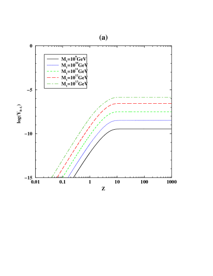
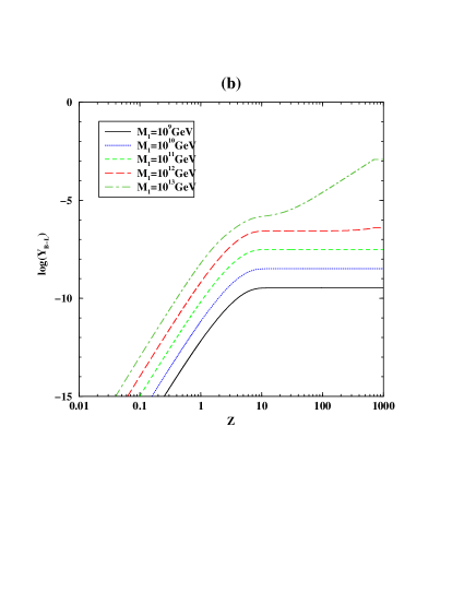
Figure 7.2: The evolution of B-L asymmetry with maximal allowed $CP$ violation parameter $\epsilon_{1}$ for different values of $M_{1}$, with $\tilde{m}_{1}=10^{-4}eV$ and $\eta_{B-L}=10^{13}GeV$ (a) in absence of cosmic strings, and (b) in presence of cosmic strings.

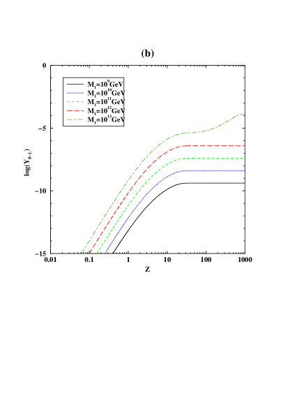
Figure 7.3: The evolution of B-L asymmetry with maximal allowed $CP$ violation parameter $\epsilon_{1}$ for different values $M_{1}$, with $\tilde{m}_{1}=10^{-5}eV$ and $\eta_{B-L}=10^{13}GeV$ (a) in absence of cosmic strings, and (b) in presence of cosmic strings.

In the usual thermal scenario the $B-L$ asymmetry depends on not only $\tilde{m}_{1}$, but also $M_{1}$. In the present case the $B-L$ asymmetry depends, additionally, on $\eta_{\rm B-L}$ since the injection rate of $N_{1}$’s from the cosmic string loops strictly depends on it. Depending on the $B-L$ symmetry breaking scale, the effects of cosmic strings on the baryon asymmetry are shown in the Figures 7.2 and 7.3. In these Figures we have taken the saturated value of the $CP$-asymmetry parameter $\epsilon_{1}$.

In Figure 7.2(a) it can be seen that in a thermal bath the $B-L$ asymmetry approaches the final value at around $M_{1}=10T$ when all the wash out processes fall out of equilibrium. In contrast to it, in the presence of cosmic strings the $B-L$ asymmetry continues to build up until the injection rate of $N_{1}$’s in a comoving volume is insignificant. For $f_{1}=1$ this happens around $M_{1}=6\times 10^{2}T$, as shown in Figure 7.2(b), which is far larger than in the purely thermal case. As a result of this, in presence of cosmic strings, for a fixed value of the symmetry breaking scale $\eta_{\rm B-L}=10^{13}\,{\rm GeV}$, the final $B-L$ asymmetry is enhanced by three orders of magnitude for the effective neutrino mass $\tilde{m}_{1}=10^{-4}eV$ (Fig. 7.2(b)) and by two orders of magnitude for $\tilde{m}_{1}=10^{-5}eV$ (Fig. 7.3(b)). For $f_{1}<0.01$ the effect of cosmic string essentially disappears.

The above happenings, in particular the dependence on the value of $\tilde{m}_{1}$, can be understood as follows: In the absence of injection term when the wash out processes fall out of equilibrium the asymmetry produced by the decay of $N_{1}$’s does not get wiped out, and the produced $B-L$ asymmetry remains as the final asymmetry. Since the decay rate of $N_{1}$’s depends linearly on $\tilde{m}_{1}$ as inferred from equation (4.10), a relatively larger value of $\tilde{m}_{1}$ implies that the condition of decay in out-of-equilibrium situation is satisfied at a relatively later time when the abundance of thermal $N_{1}$’s is relatively smaller, thus yielding a smaller final value of $Y_{B-L}$. And as expected, this effect is larger for larger values of $M_{1}$.

Now let us see what happens when the injection term due to the string loops is added. For values of $\eta_{B-L}$ for which the string contribution remains subdominant to the thermal contribution, the dependence on $\tilde{m}_{1}$ is essentially same as in the absence of the strings as explained above. However, the situation is reversed for those values of $\eta_{B-L}$ for which the string contributions are dominant: Since the string-produced $N_{1}$’s dominate over those of thermal origin at late times, the $B-L$ asymmetry produced by the decay of the string-produced $N_{1}$’s automatically satisfy the out-of-equilibrium condition. In such a situation, a relatively larger value of $\tilde{m}_{1}$ (implying a relatively larger rate of decay of the $N_{1}$’s) simply leads to a quicker rate of development of the $Y_{B-L}$ at a relatively earlier time when the injection rate of the $N_{1}$’s is relatively larger, thus yielding a relatively higher final value of $Y_{B-L}$. Figures 7.2(b) and 7.3(b) plotted for $\tilde{m}_{1}=10^{-4}eV$ and $\tilde{m}_{1}=10^{-5}\,{\rm eV}$ simultaneously bear out these expectations.

Allowing a maximal CP-asymmetry, we see that for a reasonable value of $\tilde{m}_{1}$ in certain models the string contribution overproduces the baryon asymmetry in comparison to the thermal value for $\eta_{\rm B-L}=10^{13}\,{\rm GeV}$ and $f_{1}\mbox{\raisebox{-2.58334pt}{~{}$\stackrel{{\scriptstyle>}}{{\sim}}$~{}}}0.1$. This suggests a lower $\eta_{\rm B-L}$ or $\delta<1$ in equation (7.20) may be in better accord with the observed baryon asymmetry in the presence of $B-L$ cosmic strings. Therefore, we have repeated the above calculations for $\eta_{\rm B-L}=10^{12}\,{\rm GeV}$ and $\eta_{\rm B-L}=10^{11}\,{\rm GeV}$. The results are summarized in tables (7.1) and (7.2). In both cases one can see that for Yukawa coupling $f_{1}<1$ and $\tilde{m}_{1}=10^{-5}\,{\rm eV}$ the effect of cosmic strings disappear, i.e. $(\Delta Y_{\rm B-L}/Y_{\rm B-L}^{th})\rightarrow 0$, where $\Delta Y_{\rm B-L}\equiv Y_{\rm B-L}^{th+st}-Y_{\rm B-L}^{th}$. This is in concordance with our assumption that $\tilde{m}_{1}\leq O(10^{-5})\,{\rm eV}$ in the given model in section 7.5.2.

Studying the needed bound on $\delta$ we find that for $\eta_{\rm B-L}=10^{13}\,{\rm GeV}$ and $M_{1}=10^{13}\,{\rm GeV}$ to produce the final $B-L$ asymmetry, $Y_{\rm B-L}^{th+st}=O(10^{-10})$, we need $\delta=O(10^{-7})$ and $O(10^{-6})$ for $\tilde{m}_{1}=10^{-4}$eV and $\tilde{m}_{1}=10^{-5}$eV respectively. These values of $\delta$ diminish the purely thermal contributions, $Y_{\rm B-L}^{th}=O(10^{-13})$ and $O(10^{-12})$ respectively. Thus there exists ranges of parameter values where, while the thermally abundant heavy neutrinos are not sufficient to produce the required $B-L$ asymmetry, the cosmic string contribution can produce the required asymmetry.

Table 7.1: Effect of cosmic strings on final $B-L$ asymmetry is shown for different values of the Yukawa coupling $f_{1}$ at $\eta_{\rm B-L}=10^{12}\,{\rm GeV}$

$f_{1}$	$\tilde{m}_{1}=10^{-4}eV$			$\tilde{m}_{1}=10^{-5}eV$
	$Y^{th}_{B-L}$	$Y^{th+st}_{B-L}$	$\log(\delta_{reqd})$	$Y^{th}_{B-L}$	$Y^{th+st}_{B-L}$	$\log(\delta_{reqd})$
1	$2.721\times 10^{-7}$	$1.231\times 10^{-5}$	$-5$	$3.903\times 10^{-7}$	$1.594\times 10^{-6}$	-4
0.1	$3.098\times 10^{-8}$	$3.218\times 10^{-8}$	$-2$	$3.970\times 10^{-8}$	$3.982\times 10^{-8}$	$-2$
0.01	$3.254\times 10^{-9}$	$3.254\times 10^{-9}$	$-1$	$4.038\times 10^{-9}$	$4.038\times 10^{-9}$	-1
0.001	$3.393\times 10^{-10}$	$3.393\times 10^{-10}$	0	$4.107\times 10^{-10}$	$4.107\times 10^{-10}$	0

Table 7.2: Effect of cosmic strings on final $B-L$ asymmetry is shown for different values of the Yukawa coupling $f_{1}$ at $\eta_{\rm B-L}=10^{11}\,{\rm GeV}$

$f_{1}$	$\tilde{m}_{1}=10^{-4}eV$			$\tilde{m}_{1}=10^{-5}eV$
	$Y^{th}_{B-L}$	$Y^{th+st}_{B-L}$	$\log(\delta_{reqd})$	$Y^{th}_{B-L}$	$Y^{th+st}_{B-L}$	$\log(\delta_{reqd})$
1	$3.098\times 10^{-8}$	$1.514\times 10^{-7}$	-3	$3.970\times 10^{-8}$	$5.174\times{-8}$	-2
0.1	$3.254\times 10^{-9}$	$3.266\times 10^{-9}$	$-1$	$4.038\times 10^{-8}$	$4.039\times 10^{-9}$	$-1$
0.01	$3.392\times 10^{-10}$	$3.392\times 10^{-10}$	0	$4.107\times 10^{-10}$	$4.107\times 10^{-10}$	0

While the mechanism investigated here can be easily generalized to a supersymmetric model, there are unlikely to be significant changes in the quantitative aspects. In particular unless some salient physics significantly modifies the scale of efficacy, viz., $10^{11}\,{\rm GeV}$ of this mechanism, the supersymmetric generalization is not helpful in resolving the issue raised by the gravitino bound and the need for a mechanism at scales $<10^{9}\,{\rm GeV}$.

A more fruitful approach towards success of this scenario at lower energy scales would be to also seek additional sources for $CP$ violation for the cosmic string generated heavy neutrinos. This is possible since they get produced from the decay of a bosonic condensate consisting of the string loops. However the strength of the present investigation is the direct comparison between the two sources of heavy neutrinos. If the mechanism applicable to the non-thermal source is different, the model becomes less constrained and its verifiability is sacrificed to a certain extent.

A useful conclusion from the rather constrained scenario considered here is that in the regime $\eta_{\rm B-L}>10^{11}\,{\rm GeV}$ and $h_{1}\mbox{\raisebox{-2.58334pt}{~{}$\stackrel{{\scriptstyle>}}{{\sim}}$~{}}}0.01$ for $\epsilon_{1}\ll\epsilon_{1}^{max}$ (i.e. $\delta\ll 1$) while the thermal abundance of right handed neutrinos is not sufficient to produce the required $B-L$ asymmetry the cosmic strings can give rise to the observed level of the asymmetry.

Chapter 8 Conclusions

Baryogenesis via leptogenesis is an attractive scenario that links the physics of right handed neutrino sector with the low energy neutrino data. In the light of current neutrino oscillation data we studied the bounds on the mass scale of lightest right handed neutrino as well as their mass hierarchy from the leptogenesis constraint which we discuss in two different parts of the thesis. In part-I, we study the baryogenesis via leptogenesis in a thermal scenario, while part-II of the thesis is devoted to a study of the same in a non-thermal scenario. Moreover, we divide the phenomenological models into two categories, type-I and type-II, depending on the seesaw mechanism used to generate the light Majorana neutrino masses.

In Part-I, we begin with a brief introduction to type-I models. As an example, we consider a minimal extension of the $SM$ with the gauge group $SU(2)_{L}\times U(1)_{Y}\times U(1)_{Y^{\prime}}$, where $Y^{\prime}$ is a linear combination of $Y$ and $B-L$. Since $B-L$ is a gauge symmetry of the model any pre-existing asymmetry is washed out. A net asymmetry is generated when $B-L$ symmetry breaks. In such models, the right handed heavy Majorana neutrinos, $N_{i}$ with $i=1,2,3$, are singlet under the $SM$ gauge group $SU(2)_{L}\times U(1)_{Y}$. The type-I seesaw mechanism then gives rise to the light Majorana neutrino mass matrix, $m_{\nu}=m_{D}^{T}M_{R}^{-1}m_{D}$, with $m_{D}$ is the Dirac mass matrix of the neutrinos. In these models, we briefly discussed the baryogenesis via the route of leptogenesis in a thermal scenario. The leptogenesis occurs via the out of equilibrium decay of thermally generated heavy Majorana neutrinos. We assume that the mass spectrum of right handed Majorana neutrinos is in normal hierarchy. In this scenario, the final lepton asymmetry is given by the $CP$-violating decays of the lightest right handed neutrino $N_{1}$ to $SM$ Higgs and lepton. A part of this asymmetry is then transformed to the $B$-asymmetry through the equilibrated sphaleron processes.

The $L$-asymmetry predicted by a model is a measure of the magnitude of $CP$-violation in that model. The theoretical upper bound on the $CP$-asymmetry, produced by the decay of $N_{1}$, in type-I models is given by $\epsilon_{1}$ $\leq(3M_{1}/16\pi v^{2})$$\sqrt{\Delta m^{2}_{atm}}$, with $\Delta m^{2}_{atm}$ is the mass squared difference of light neutrinos in atmospheric data. The analytical estimation of $L$-asymmetry in these models recasts the upper bound on $CP$-asymmetry in terms of a lower bound on the mass scale of $N_{1}$ to be $M_{1}\geq 10^{9}GeV$. In the light of current neutrino oscillation data we numerically check the compatibility of the analytical ound on $M_{1}$ by solving the required Boltzmann equations.

The $B-L$ gauge symmetry in the given example of type-I model is quite ad hoc. We therefore consider models where $B-L$ gauge symmetry emerges naturally. In particular, we consider Left-Right symmetric model, a specific example of type-II seesaw models. The scalar sector of the model is very rich and consists of two triplets, namely $\Delta_{L}$ and $\Delta_{R}$, and a bidoublet Higgs $\Phi$, which contains two copies of $SM$ Higgs. The type-II seesaw mechanism in this model gives rise the Majorana mass matrix of the light neutrinos of the form $m_{\nu}=M_{L}-m_{D}M_{R}^{-1}m_{D}^{T}$. In contrast to type-I models, in the present case the additional mass, $M_{L}$, is provided by the vacuum expectation value of the triplet $\Delta_{L}$. The two terms, $M_{L}\equiv m_{\nu}^{II}$ and $m_{D}M_{R}^{-1}m_{D}^{T}\equiv m_{\nu}^{I}$, contributing to $m_{\nu}$ are called type-II and type-I respectively. In these models, irrespective of the magnitudes of type-I and type-II terms, we show that the lower bound on $M_{1}$ can be reduced by an order of magnitude in comparison to type-I case.

Within the Left-Right symmetric model, we consider a special case in which the $CP$-violation arises through the spontaneous symmetry breaking. The Lagrangian of the model is $CP$ invariant which demands that all the Yukawa couplings should be real. In this scenario, the vacuum expectation values ($VEV$s) of the neutral Higgses are complex and they lead to complex masses for fermions and hence $CP$-violation. In the Left-Right symmetric model, there are four complex neutral scalars which acquire VEVs. However, the unbroken global $U(1)$ symmetries associated with $SU(2)_{L}$ and $SU(2)_{R}$ gauge groups allow two of the phases to be set to zero. Using the remnant $U(1)$ symmetry after the breaking of $SU(2)_{R}$, one phase choice is made to make the $VEV$ of $\Delta_{R}$, and hence the mass matrix of right handed neutrinos, real. The phase associated with the other $U(1)$ symmetry can be chosen to achieve two different types of simplification of neutrino mass matrix. In the type-II choice, the $m_{\nu}^{I}$ is made real leaving the $CP$-violating phase purely with $m_{\nu}^{II}$. In this phase convention, we derive a lower bound on the mass scale of $N_{1}$ from the leptogenesis constraint by assuming a normal mass hierarchy in the right handed neutrino sector. It is shown that the mass scale of $N_{1}$ satisfy the constraint $M_{1}\geq 10^{8}GeV$, which is in good agreement with the lower bound on $M_{1}$ in generic type-II seesaw models. In the type-I phase choice, only the type-I term contains $CP$-violating phase leaving type-II term real. This allows us to derive an upper bound on the heavy neutrino mass hierarchy from the leptogenesis constraint. In order to achieve the observed baryon asymmetry of the present Universe, it is found that the mass hierarchy of right handed neutrinos satisfy the constraint $M_{2}/M_{1}\leq 17$ and $M_{3}/M_{1}\leq 289$ simultaneously. Numerically we verified that these bounds are compatible with the low energy neutrino oscillation data for all values of $M_{1}\geq 10^{8}GeV$ as implied by the lower bound on $M_{1}$ in type-II phase convention. The bound on $M_{1}$, in production of $L$-asymmetry through the $CP$-violating decays of thermally generated $N_{1}$, is $\geq 10^{8}GeV$ which is far above the current accelerator energy range and beyond the reach of the next generation accelerators. However, these scenarios are well motivated by the current status of low energy neutrino oscillation data.

As an alternative, we consider mechanisms which work at $TeV$ scale and be consistent with the low energy neutrino data. We study a general scenario for $TeV$ scale leptogenesis in a gauged $B-L$ symmetric model. By solving the Boltzmann equations we explore the viable regions in the plane of the effective neutrino mass arameter $\tilde{m}_{1}$ and the mass of lightest right handed neutrino $M_{1}$. We assume that the required lepton asymmetry of the present Universe is produced during the $B-L$ gauge symmetry breaking phase transition. The limited erasure by the processes mediated by $N_{1}$ requires that $\tilde{m}_{1}<10^{-3}eV$. Solution of the relevant Boltzmann equations shows that for $\tilde{m}_{1}=10^{-4}eV$ the mass of $N_{1}$ has to be smaller than $10^{12}GeV$ and can be as low as $10TeV$. In a more restrictive scenario where the neutrino Dirac mass matrix is identified with that of the charged leptons it is necessary that $M_{1}>10^{8}GeV$ in order to satisfy $\tilde{m}_{1}<10^{-3}eV$. In this scenario all values $M_{1}$, $10^{8}GeV<M_{1}<10^{12}GeV$ can successfully create the required asymmetry. If the Dirac mass scale of neutrinos is less restricted, much lower values of $M_{1}$ are allowed. In particular, a right handed neutrino as low as $10TeV$ is admissible if the Dirac mass scale is about a factor of $100$ smaller than the mass scale of charged leptons. We conjecture that the hypothesis of $TeV$ scale right handed neutrinos can be verified in the near future, thus providing an indirect evidence of baryon asymmetry creation at $TeV$ scale.

In part-II of the thesis, we discuss the formation and evolution of topological defects, in particular cosmic strings, in the early Universe. Topological defects arise as the solitonic solutions in gauge theories. ‘Solitons’ or ‘solitary waves’ are the time independent solutions of non-linear wave equations in classical field theories. The prime among them is $\lambda\phi^{4}$ theory. In 1+1-dimensions the solitonic solutions in $\lambda\phi^{4}$ theory are called ‘kinks’. Each solitonic solution is designated by a number called the ‘topological charge’ or ‘winding number’.

An inevitable feature of the early Universe phase transitions is the formation of topological defects. In particular, we deal with cosmic strings. These defects are extended objects and are not distributed thermally. Therefore, the decay of these objects can be a non-thermal source of massive particles that constitutes them. Moreover, the cosmic strings formed at a phase transition can also influence the nature of a subsequent phase transition that may have important implications for the generation of Baryon Asymmetry of the Universe ($BAU$).

In Quantum Field Theory ($QFT$), solutions of Dirac equation in the presence of solitonic objects lead to a curious phenomenon of ‘fractional fermion number’. This is because of the existence of degenerate zero energy modes of fermions while quantized in the background of a solitonic vacuum. In contrast to it, in the translational invariant vacuum there are no zero energy solutions of Dirac equation and therefore fermions are quantized by integral unit. The fractional solitonic states are therefore superselected from the normal vacuum and are not allowed to decay in isolation.

An important feature of cosmic strings is that during their formation they trap zero energy modes of fermions. These fermionic zero modes induce fractional fermion number ($|n|/2$) on a string of winding number $n$. If $n$ is odd then the induced fermion number on the string is half-integral. Therefore, it is superselected from the translation invariant vacuum where the eigenvalues of the number operator carry integral fermion number. Thus, a string of half integer fermion number can not decay in isolation because of the unavailability of fractional fermion states in the translational invariant vacuum. We construct examples where metastable infinitely long cosmic strings enjoy stability due to this quantum mechanical phenomenon.

There exist both analytical as well as numerical studies of the evolution of cosmic strings network in the early Universe. These suggest that the strings network quickly enters a scaling regime in which the energy density of the strings scales as a fixed fraction of the energy density of radiation in the radiation dominated epoch, or the energy density of matter in the matter dominated epoch. In both cases the energy density scales as $t^{-2}$. In this regime one of the fundamental physical process that maintains the strings network to be in that configuration is the formation of sub-horizon size closed loops which are pinched off from the network whenever a string segment curves over into a loop, intersecting itself.

There have been many scenarios that consider decaying, collapsing, or repeatedly self-intersecting closed loops of such cosmic strings providing a non-thermal source of massive particles that “constitute” the string. The decay of these massive particles gives rise to the observed $B$-asymmetry or a significant fraction of it. We have estimated the contribution to $BAU$ from cosmic string loops which disappear through the process of (a) slow shrinkage due to energy loss through gravitational radiation — which we call slow death (SD), and (b) repeated self-intersections — which we call quick death (QD). We find that for reasonable values of the relevant parameters, the SD process dominates over the QD process as far as their contribution to $BAU$ is concerned. We assume that the final demise of each string loop in the SD process produces $O(1)$ right handed neutrino, $N_{1}$. We demand that the $B$-asymmetry, produced by the decay of non-thermally generated $N_{1}$’s through the leptogenesis route, should not exceed the observed value predicted by WMAP. This requires that the mass scale of $N_{1}$ satisfy the constraint $M_{1}\leq 2.4\times 10^{12}\left(\eta_{\rm B-L}/10^{13}GeV\right)^{1/2}GeV$, where $\eta_{\rm B-L}$ is the scale of $U(1)_{\rm B-L}$ gauge symmetry breaking phase transition. This in turn constrains the $B-L$ symmetry breaking scale to be $\eta_{\rm B-L}\geq 5.6\times 10^{11}GeV$ unless the Majorana Yukawa coupling of $N_{1}$ is allowed to be greater than unity. In this analytical approximation we have assumed that above the mass scale of $N_{1}$ there is no lepton asymmetry. A net lepton asymmetry has been produced just below the mass scale of $N_{1}$ by it’s $CP$-violating decays to $SM$ Higgs and lepton. We then checked the analytical results against the numerical smulations. This is done by solving the relevant Boltzmann equations and including the effects of both thermal and string generated right handed neutrinos. We explored the parameter region spanned by the relevant light- and heavy neutrino mass parameters $\tilde{m}_{1}$ and $M_{1}$, and constrained the scale of $B-L$ symmetry breaking, $\eta_{B-L}$, as well as the Majorana Yukawa coupling $f_{1}$ of the lightest right handed neutrino. It is shown that for the values $\eta_{B-L}>10^{11}$GeV, where they can be effective, cosmic strings make a more dominant contribution than thermal leptogenesis. This, in turn, provides an upper bound on the $CP$ violating phase giving rise to the $L$-asymmetry.

Appendix A The Boltzmann equations

A.1 Particle distribution in thermal plasma

Let $f_{i}(\vec{p},t)$ be the density distribution of the particle species $i$ in phase space. Assuming that the Universe is isotropic $f_{i}$ can be chosen to be independent of the position vector $\vec{r}$. In the high temperature thermal bath it is assumed that all species of particles in the Universe were initially in thermal equilibrium and spread homogeneously. The only deviation comes for the massive particles as the Universe expands. The expansion of the Universe causes the momenta of all particles to redshift, so that $p\sim\frac{1}{R}$. So long as the energy density of the Universe is dominated by the ultra relativistic particle species the temperature of the Universe will like wise redshift as $T\sim\frac{1}{R}$. Thus the distribution function, $f_{i}$, is simply given by

$$f_{i}(\vec{p})=e^{-\frac{|\vec{p_{i}}|}{T}}$$ (A.1)

where $i$ stands for the particle species. However, for massive particles the distribution function must be

$$f_{i}(\vec{p})=e^{-\frac{\sqrt{|\vec{p_{i}}|^{2}+M_{i}^{2}}}{T}}.$$ (A.2)

In the configuration space the number density of the of the particle species $i$ is

$$n_{i}=g_{i}\int\frac{d^{3}\vec{p}}{(2\pi)^{3}}f_{i}(\vec{p})$$ (A.3)

where $g_{i}$ is the number of accessible spin states for the particle species $i$. Thus for a massless thermal photon($\gamma$), the density distribution, given by equation (A.3), is

$$n_{\gamma}=\frac{2}{\pi^{2}}T^{3}.$$ (A.4)

Far above their mass scales the massive particles are in thermal equilibrium. Therefore, the phase space distribution function is given by

$$f_{i}^{eq}=e^{-\frac{E_{i}}{T}},$$ (A.5)

where $E_{i}=\sqrt{|p_{i}|^{2}+M_{i}^{2}}$. So the equilibrium density distribution is

$$n_{i}^{eq}=g_{i}\int\frac{d^{3}p_{i}}{(2\pi)^{3}}f_{i}^{eq}$$ (A.6)

In terms of the dimensionless variables $x=\frac{\sqrt{|p_{i}|^{2}+M_{i}^{2}}}{T}$ and $Z=\frac{M_{i}}{T}$, equation (A.6) can be rewritten as

$$n_{i}^{eq} = g_{i}\frac{T^{3}}{2\pi^{2}}\int_{Z}^{\infty}xe^{-x}\sqrt{x^{2}-Z^{2}}dx$$ (A.7)

$$= g_{i}\frac{T^{3}}{2\pi^{2}}Z^{2}K_{2}(Z)$$

where $K_{2}(Z)$ is modified Bessel function. As $Z\rightarrow 0$, $z^{2}K_{2}(Z)\rightarrow 2$. In this limit, the density distribution of massive particles resembles with mass less particles. Thus the approximation that at a temperature above their mass scale all particles are in thermally equilibrium is a valid assumption. As the Universe expands the temperature falls ($Z$ increases). Therefore, the density distribution of all particles fall and is governed by the Boltzmann transport equations.

A.2 Boltzmann transport equations

In this section, we give a pragmatic introduction to Boltzmann equations to study the evolution of the density of any particle species in the absence and presence of interactions.

The expansion of the Universe dilutes the number densities of all types of particles even in the absence of interactions at a rate

$$\frac{dn_{i}}{dt} = -3\frac{\dot{R}}{R}n_{i}$$ (A.8)

$$= -3Hn_{i}$$

where $R(t)$ is scale factor in Freedman Robertson and Walker (FRW) Universe and $\dot{R}$ is derivative with respect to time. $H$ is Hubble expansion factor. Thus in the absence of any interaction the Boltzmann transport equation for the given particle species $i$ of density $n_{i}$ is

$$\frac{dn_{i}}{dt}+3Hn_{i}=0.$$ (A.9)

Now we scale out the effect of the expansion of the Universe by considering the evolution of the number of particles in a comoving volume. This can be done by dividing the number density of the particle species $i$ with its entropy density, i.e.

$$Y_{i}=\frac{n_{i}}{s}.$$ (A.10)

Using the conservation of entropy per comoving volume ($sR^{3}$ = constant), equation (A.10) can be written as

$$\frac{dn_{i}}{dt}+3Hn_{i}=s\dot{Y}=0.$$ (A.11)

As the Universe expands the momentum $p_{i}$ of the particle species $i$ falls as $1/R$ and thus also the temperature $T$. Under rescaling the momenta of massless particles remain unchanged. So they keep themselves in equilibrium with the thermal plasma. Above the mass scale of any massive particle it will behave as a massless one. Below its mass scale the interaction rate decreases in comparison to the Hubble expansion rate and hence it falls out of equilibrium because it needs several collision times to keep it in equilibrium with the thermal photons. The departure of the density of any species $i$ from its thermal equilibrium value can be predicted by solving the Boltzmann transport equations.

For simplicity we consider the decay of any massive species $i$ to a set of particles $Y$. As a result the equation (A.11 modifies to

$$\frac{dn_{i}}{dt}+3Hn_{i}=-\sum_{i\leftrightarrow Y}\left[\frac{n_{i}}{n_{i}^{eq}}\gamma(i\rightarrow Y)-\frac{n_{Y}}{n_{Y}^{eq}}\gamma(Y\rightarrow i)\right],$$ (A.12)

where

$$\gamma(i\rightarrow Y)=\int d\Pi_{i}d\Pi_{Y}(2\pi)^{4}\delta^{4}(p_{i}-p_{Y})f_{i}^{eq}|\mathcal{A}(i\rightarrow Y)|^{2}.$$ (A.13)

In equation (A.13), $d\Pi=\frac{1}{2E}\frac{d^{3}p}{(2\pi)^{3}}$. If we neglect $CP$-violation then $|\mathcal{A}(i\rightarrow Y)|^{2}=|\mathcal{A}(Y\rightarrow i)|^{2}$. Using (A.6) the above equation (A.12) simplifies to

$$\frac{dn_{i}}{dt}+3Hn_{i}=-\Gamma_{D}(n_{i}-n_{i}^{eq}),$$ (A.14)

where we have used

$$\Gamma_{D}=\frac{1}{2E_{i}}\int\frac{d^{3}p_{Y}}{(2\pi)^{3}2E_{Y}}(2\pi)^{4}\delta^{4}(p_{i}-p_{Y})|\mathcal{A}|^{2}.$$ (A.15)

Note that in the above simplification we have assumed $n_{Y}=n_{i}^{eq}$ and it is true because the decay products $Y$ are massless till the later epochs of our interest. Substituting $Z=M_{i}/T$ and $Y_{i}=n_{i}/s$ in equation (A.12) we get

$$\frac{dY_{i}}{dZ} = -\frac{\Gamma_{D}}{ZH(Z)}(Y_{i}-Y_{i}^{eq})$$ (A.16)

$$= -D(Y_{i}-Y_{i}^{eq}).$$

Considering the $2\leftrightarrow 2$ scatterings involving the species $i$ equation (A.16) can be extended to

$$\frac{dY_{i}}{dZ}=-(D+S)(Y_{i}-Y_{i}^{eq}),$$ (A.17)

where $S=\Gamma_{s}/ZH$. This is the final Boltzmann equation for the evolution of any species $i$ due to its decay and scatterings.

Appendix B Homotopy theory

In the following we discuss some of the fundamental definitions which are useful for our purpose.
Path: A path $f$ in a manifold $M$ is defined as a continuous function $f(t)$ of a real parameter $t$, so that each value of $t$ in the interval $0\leq t\leq 1$ corresponds to a point $f(t)$ in the manifold $M$. If a path $f(t)$ connects the points $P$ and $Q$ we have $f(0)=P$, $f(1)=Q$. If $f(0)=f(1)=P$ we have a closed path. On the other hand, if $f(0)\neq f(1)$ then the path is ${\it open}$.
Inverse of a path $f$ is written as $f^{-1}$ and is defined as

$$f^{-1}(t)=f(1-t),$$ (B.1)

so that it corresponds to the same path traversed in the opposite direction.
Product of two paths $f$ and $g$ is written as $h=fg$ and is given by

$$h(t) = f(2t)\hskip 28.45274ptfor\hskip 14.22636pt0\leq t\leq 1/2$$

$$h(t) = f(2t-1)\hskip 28.45274ptfor\hskip 14.22636pt1/2\leq t\leq 1.$$ (B.2)

Two paths $f(t)$ and $g(t)$, both starting at $P$ and ending at $Q$($P\neq Q$), are said to be homotopic to each other if $f(t)$ is continuously deformed to $g(t)$ and is defined by $f\sim g$. More specifically we can define a function $L(s,t)$ such that $L(0,t)=f(t)$ and $L(1,t)=g(t)$.

Having defined path we shall construct a group by introducing a class of paths homotopic to $f$, denoted by $[f]$. They must, of course, have the same end-points. These homotopy classes may be multiplied, by defining the multiplication law

$$[f][g]=[fg].$$ (B.3)

It is easy to see that, this multiplication law defines a group, called the fundamental group or first homotopy group of the manifold $M$, and denoted by $\pi_{1}(M)$. This requires the four properties that satisfied by a group. They are:
1.   Closure: If $[f]\in\pi_{1}(M)$ and $[g]\in\pi_{1}(M)$, then adhering to (B.3) $[f][g]\in\pi_{1}(M)$.
2.    Associativity: Since $(fg)h\sim f(gh)$ we have $([f][g])[h]=[f]([g][h])$.
3.   Identity element: This is the class of paths[I] that can be shrunk to a point.
4.   Inverse: Since $[f^{-1}][f]=[I]$, so $[f]^{-1}=[f^{-1}]$

The manifold $M$ is said to be a simply connected if all the closed paths in that manifold can be shrunk to a point. On the other hand, if all paths can not be shrunk to a point then, the Manifold is path connected.

Bibliography

- [1] A.D. Sakharov, JETP Lett. 5, 24 (1967).
- [2] M. Yoshimura, Phys. Rev. Lett. 41, 281 (1978); erratum, 42, 740 (1979).
- [3] S. Weinberg, Phys. Rev. Lett. 42, 850 (1979)
- [4] A.G. Cohen, D.B. Kaplan and A.E. Nelson Ann. Rev. Nucl. Part. Sci. 42:27-70, (1993).
- [5] M. Trodden, Rev. Mod. Phys. 71, 1463 (1996).
- [6] U.A. Yajnik, Pramana, 54, 471 (2000).
- [7] K. Jansen, Nucl. Phys. B (proc. suppl.) 47, 196, 1996.
- [8] M. Fukugita and T. Yanagida, Phys. Lett. B 174, 45 (1986).
- [9] M.A. Luty, Phys. Rev. D 45, 455 (1992).
- [10] R.N. Mohapatra and X. Zhang, Phys. Rev. D 46, 5331 (1992).
- [11] M. Plumacher, Z.phy.C 74, 549 (1997).
- [12] V.A. Kuzmin, V.A. Rubakov and M.E. Shaposhnikov Phys. Lett. B 155, 36 (1985).
- [13] P.A. Arnold and L. Mc Lerran, Phys. Rev. D 36, 581 (1987); Phys. Rev. D 37, 1020 (1988)
- [14] J. Ambjorn, T. Askgaard, H. Porter and M.E. Shaposhnikov, Phys. Lett. B 244, 479 (1990); Nucl. Phys. B 353, 346 (1991)
- [15] S.N. Ahmed et al (SNO collaboration), arXiv:nucl-ex/0309004; Q.R. Ahmed et al, Phys.Rev.Lett. 89, 011301-011302 (2002); J.N. Bahcall and C. Pena-Garay, [arXiv:hep-ph/0404061].
- [16] S. Fukuda et al. (Super-Kamiokande Collaboration) Phys. Rev. Lett. 86, 5656 (2001).
- [17] K. Eguchi et al (KamLAND collaboration), Phys. Rev. Lett. 90, 021802 (2003).
- [18] M. Gell-Mann, P. Ramond and R. Slansky in Supergravity (P. van Niewenhuizen and D. Freedman, eds), (Amsterdam), North Holland, 1979; T. Yanagida in Workshop on Unified Theory and Baryon number in the Universe (O. Sawada and A. Sugamoto, eds), (Japan), KEK 1979; R. N. Mohapatra and G. Senjanovic, Phys. Rev. Lett. 44, 912 (1980).
- [19] R. Slansky, Phys. Rep. 79, 1(1981).
- [20] M. Magg and C. Wetterich, Phys. Lett. B 94, 61 (1980).
- [21] C. Wetterich, Nucl. Phys. B 187, 343 (1981).
- [22] R.N. Mohapatra and G. Senjanovic Phys. Rev. D23, 165 (1981).
- [23] G. Lazarides, Q. Shafi and C. Wetterich, Nucl. Phys. B 181, 287 (1981).
- [24] R.N. Mohapatra,Unification And Supersymmetry, (Springer-Verlag, New-York, 1992).
- [25] E.K. Akhmedov, M. Frigerio and A.Y. Smirnov, JHEP 0309, 021 (2003)[arXiv:hep-ph/0305322], G.C. Branco, R. Gonzalez Felipe, F.R. Joaquim, M.N. Rebelo, Nucl. Phys. B640 202-232,2002,[arXiv: hep-ph/0202030]. D. Falcone, Phys. Rev. D 68, 033002 (2003) [arXiv:hep-ph/0305229].
- [26] D. Falcone and F. Tramontano, Phys. Rev. D 63, 073007 (2001) [arXiv:hep-ph/0011053]. A. S. Joshipura, E. A. Paschos and W. Rodejohann, Nucl. Phys. B 611, 227 (2001) [arXiv:hep-ph/0104228]. JHEP 0108, 029 (2001) [arXiv:hep-ph/0105175]. G. C. Branco, M. N. Rebelo and J. I. Silva-Marcos, arXiv:hep-ph/0510412. G. C. Branco, R. Gonzalez Felipe, F. R. Joaquim, I. Masina, M. N. Rebelo and C. A. Savoy, Phys. Rev. D 67, 073025 (2003) [arXiv:hep-ph/0211001]. S. Pascoli, S. T. Petcov and W. Rodejohann, Phys. Rev. D 68, 093007 (2003) [arXiv:hep-ph/0302054].
- [27] S. Davidson and A. Ibarra, Phys. Lett. B 535, 25 (2002). [arXiv:hep-ph/0202239]
- [28] W. Buchmuller, P. Di Bari and M. Plumacher, Nucl. Phys. B 643, 367 (2002). [arXiv:hep-ph/0205349].
- [29] K. Hamaguchi, H. Murayama and T. Yanagida, Phys. Rev. D 65, 043512 (2002).
- [30] T. Hambye et.al.[arXiv:hep-ph/0312203].
- [31] S. Antusch and S.F. King, Phys. Lett. B 597, 199 (2004) [arXiv:hep-ph/0405093].
- [32] N. Sahu and S. Uma Sankar, Phys. Rev. D71, 2005 (013006), [arXiv:hep-ph/0406065].
- [33] N. Sahu and S. Uma Sankar, Nucl. Phys. B 724,329 (2005), [arXiv: hep-ph/0501069].
- [34] G. Senjanovic, Nucl. Phys. B 153, 334 (1979); A. Masiero, R. N. Mohapatra and R. D. Peccei, Nucl. Phys. B 192 (1981) 66, J. Basecq, J. Liu, J. Milutinovic and L. Wolfenstein, Nucl. Phys. B 272, 145 (1986). N.G. Deshpande, J. F. Gunion, B. Kayser and F. I. Olness, Phys. Rev. D 44, 837 (1991); G. Barenboim and J. Bernabeu, Z. Phys. C 73 (1997) 321 [arXiv:hep-ph/9603379], Y. Rodriguez and C. Quimbay, Nucl. Phys. B 637, 219 (2002) [arXiv:hep-ph/0203178].
- [35] L. Boubekeur, T. Hambye and G. Senjanovic, Phys. Rev. Lett. 93, 111601 (2004) [arXiv:hep-ph/0404038]; A. Pilaftsis, T.E.J Underwood, Nucl.Phys. B692, 303-345 (2004), [arXiv:hep-hep/0309342]; T. Hambye, J.M. Russel, S.M. West, JHEP 0407, 070 (2004), [arXiv:hep-ph/0403183]. E.J. Chun, [arXiv: hep-ph/0508050] S. Dar, Q. Shafi and A. Sil, [arXiv:hep-ph/0508037]. A. Abada, H. Aissaoui and M. Losada, Nucl. Phys. B 728, 55 (2005)[arXiv:hep-ph/0409343].
- [36] S.J. Huber, M.G. Schmidt, Nucl. Phys. B 606, 83 (2001).
- [37] S.A. Abel, S. Sarkar, R.L. White, Nucl. Phys. B 454, 663-681 (1995).
- [38] C. Panagiotakopoulos, K. Tamvakis, Phys. Lett. B 446,224 (1999).
- [39] C. Panagiotakopoulos, K. Tamvakis, Phys. Lett. B 469,145, (1999).
- [40] C. Panagiotakopoulos, A. Pilaftsis, Phys. Rev. D 63 (2001) 055003.
- [41] A. Dedes, C. Hugonie, S. Moretti, K. Tamvakis, Phys. Rev. D 63, 055009 (2001).
- [42] A. Menon, D.E. Morrissey, C.E.M. Wagner, Phys. Rev. D 70, 035005 (2004), [arXiv:hep-ph/0404184].
- [43] N. Sahu and U.A. Yajnik, Phy. Rev. D71, 023507 (2005),[arXiv:hep-ph/0410075]; [arXiv:hep-ph/0509285].
- [44] J.A. Harvey and M.S. Turner, Phys. Rev. D 42, 3344 (1990).
- [45] W. Fischler, G.F. Guidice, R.G. Leigh and S. Pawan, Phys. Lett. B 258 45 (1991).
- [46] A. Vilenkin and E.P.S. Shellard, Cosmic strings and other topological defects (Cambridge University Press, 1994).
- [47] R. Jackiw and C. Rebbi, Phys Rev. D 13, 3398 (1976).
- [48] S.B. Duari and U.A. Yajnik, Phys. Lett. B 326 21 (1994).
- [49] R.H. Brandenberger, A.C. Davis, and M. Trodden, Phys. Lett. B 335 123 (1994).
- [50] R. Jackiw and P. Rossi, Nucl. Phys. B 190, 681 (1981).
- [51] E.J. Weinberg, Phys. Rev. D 24, 2669 (1981).
- [52] N. Sahu and U.A. Yajnik, Phys. Lett. B 596, 1 (2004).
- [53] P. Bhattacharjee, T.W.B. Kibble and N. Turok, Phys. Lett. B 119, 95 (1982).
- [54] R.H. Brandenberger, A.C. Davis and M. Hindmarsh, Phys. Lett. B 263, 239 (1991).
- [55] H. Lew and A. Riotto, Phys. Rev. D 49, 3837 (1994).
- [56] R. Jeannerot, Phys. Rev. Lett. 77, 3292 (1996).
- [57] P. Bhattacharjee, Phys. Rev. Lett. 81, 260 (1998).
- [58] P. Bhattacharjee, N. Sahu and U.A. Yajnik; Phys. Rev. D 70, 083534 (2004), [arXiv:hep-ph/0406054];
- [59] G.F. Giudice, A. Notari, M. Raidal, A. Riotto and A. Strumia, Nucl. Phys. B 685, 89 (2004), [arXiv:hep-ph/0310123];
- [60] N. Sahu, P. Bhattacharjee, U.A. Yajnik, [arXiv:hep-ph/0512350].
- [61] Z. Maki, M. Nakagawa and S. Sakata, Prog. Theor. Phys. 28, 870 (1962); B. Pontecorvo, Sov. Phys. JETP 7, 172 (1958) [Zh. Eksp. Teor. Fiz. 34, 247 (1957)]. B. Pontecorvo, Sov. Phys. JETP 6, 429 (1957) [Zh. Eksp. Teor. Fiz. 33, 549 (1957)].
- [62] M. Flanz, E. A. Paschos, U. Sarkar and J. Weiss, Phys. Lett. B 389 (1996) 693 [arXiv:hep-ph/9607310]. M. Flanz, E. A. Paschos and U. Sarkar, Phys. Lett. B 345 (1995) 248 [Erratum-ibid. B 382 (1996) 447] [arXiv:hep-ph/9411366]. L. Covi, E. Roulet and F. Vissani, Phys. Lett. B 384, 169 (1996) [arXiv:hep-ph/9605319].
- [63] D.N. Spergel et. al. Astrophys.J.Suppl. 148 (2003) 175 [astro-ph/0302209].
- [64] W. Buchmuller, C. Greub and P. Minkwoski, Phys. Lett. B267, 395 (1991).
- [65] P. O’Donnell and U. Sarkar, Phys. Rev. D 49 (1994) 2118.
- [66] G. Lazarides and Q. Shafi, Phys. Rev. D 58 (1998) 071702.
- [67] T. Hambye and G. Senjanovic, Phys. Lett. B 582, 73 (2004).
- [68] P. Ball, J.M. Frere and J. Matias, Nucl. Phys. B 572, 3 (2000).
- [69] M.C. Chen and K.T. Mahanthappa, [arXiv:hep-ph/0411158].
- [70] H. Fritzsch, Nucl. Phys. B155, 189 (1979).
- [71] S.M. Bilenky, J. Hosek and S.T. Petcov, Phys. Lett. B94, 495 (1980).
- [72] W. Rodejohann, Nucl. Phys. B 597, 110 (2001).
- [73] M.C. Gonzalez-Garcia and C. Pena-Garay, Phys. Rev.D 68, 093003 (2003).
- [74] N. Nimai Singh, M. Patagiri, Mrinal Das, [arXiv:hep-ph/0406075].
- [75] M. Plumacher, Nucl. Phys. B 530, 207 (1998).
- [76] J.M. Cline, U.A. Yajnik, S.N. Nayak and M. Rabikumar, Phys. Rev. D 66, 65001 (2002); J. M. Frere, L. Houart, J. M. Moreno, J. Orloff and M. Tytgat, Phys. Lett. B 314, 289 (1993) [arXiv:hep-ph/9301228].
- [77] J.C. Pati and A. Salam, Phys. Rev. D 10, 275 (1974); R.N. Mohapatra and J.C. Pati, Phys. Rev. D11, 566(1975); Phys. Rev. D 11, 2558 (1975); R.N. Mohapatra and G. Senjanovic, Phys. Rev. D12, 1502 (1975).
- [78] W. Buchmuller, P. Di Bari and M. Plumacher, Nucl. Phys. B 665, 445 (2003) [arXiv:hep-ph/0302092]. R. Barbieri, P. Creminelli, A. Strumia and N. Tetradis, Nucl. Phys. B 575, 61 (2000) [arXiv:hep-ph/9911315];
- [79] W. Buchmuller, P. Di Bari and M. Plumacher, Annals Phys. 315, 305 (2005),[arXiv:hep-ph/0401240]
- [80] U.A. Yajnik, H. Widyan, S. Mahajan, A. Mukherjee and D. Choudhuri Phys. Rev. D 59 (1999) 103508.
- [81] T.W.B. Kibble, G. Lazarides and Q. Shafi, Phys. Rev. D 26, 435 (1982), G. Lazarides and Q. Shafi, Phys. Lett. B 159, 261 (1985).
- [82] H. Lew and A. Riotto, Phys. Lett. B 309, 258 (1993).
- [83] M. Joyce, T. Prokopec and N. Turok, Phys. Rev. Lett. 75, 1695 (1995); [erratum-ibid 75,3375 (1995)].
- [84] J.M. Cline, M. Joyce and K. Kainulainen Phys. Lett. B 417 79 (1998) [erratum: arXiv:hep-ph/0110031].
- [85] J.M. Cline and K. Kainulainen Phys. Rev. Lett. 85, 5519 (2000).
- [86] R. RajaramanSolitons and Instantons (Amestradam, North Holland, 1982).
- [87] W.P. Su, J. R. Schrieffer, Nucl. Phys. B190, 253 (1981).
- [88] M.J. Rice, Phys. Lett. A71, 152 (1979).
- [89] R. Rajaraman, [arXiv:cond-mat/0103366].
- [90] R. Jackiw, hep-th/9903255.
- [91] E. Witten, Nucl. Phys. B 249,557(1985).
- [92] G.C. Wick, A.S. Wightman and E.P. Wigner, Phys. Rev. 88, 101 (1952).
- [93] J. Preskill and A. Vilenkin, Phys. Rev. D 47, 2324 (1993).
- [94] H. de Vega, Phys. Rev. D 18, 2932 (1978).
- [95] A. Stern, Phys. Rev. Lett.52, 2118(1983).
- [96] A. Stern and U.A. Yajnik, Nucl. Phys. B 267, 158 (1986), S. R. Das, Nucl. Phys. B227, 462 (1983).
- [97] N. Ganoulis, G. Lazarides, Phys. Rev. D 38 547 (1988).
- [98] R.F. Dashen, B. Hasslacher and A. Neveu Phys. Rev. D 10, 4138 (1974).
- [99] C.R. Nohl, Phys. Rev. D 12, 1840 (1975) .
- [100] R. Jackiw, Rev. Mod. Phys. 49, 681(1977).
- [101] E.C.G. Sudarshan and U.A. Yajnik, Phys. Rev. D 33, 1830 (1986).
- [102] See for instance M. Fukugita and T. Yanagida, in ”Physics and Astrophysics of Neutrinos”, M. Fukugita and A. Suzuki, (eds.), Springer-Verlag, (1994), pp. 1-248.
- [103] R. MacKenzie and F. Wilczek, Phys. Rev. D 30, 2194 (1984).
- [104] S. Weinberg, The Quantum Theory of fields, Vol. I, sec. 3.3, Cambridge University Press, 1996.
- [105] S.C. Davis, W.B. Perkins and A.C. Davis, Phys. Rev. D 62, 043503 (2000)
- [106] R. Jeannerot and A.C. Davis, Phys. Rev. D 52, 7220 (1995).
- [107] R. Jeannerot Phys. Rev. D 53, 5426 (1996).
- [108] S.C. Davis, Int. J. Theor. Phys. 38, 2889 (1999); G. Starkman, D. Stojkovic and T. Vachaspati, Phys. Rev. D63, 085011 (2001), Phys. Rev. D65, 065003 (2002).
- [109] P. Bhattacharjee and G. Sigl, Phys. Rept. 327, 109 (2000).
- [110] M. Landriau and E.P.S. Shellard, Phys. Rev.D 69, 023003 (2004).
- [111] N. Bevis, M. Hindmarsh and M. Kunz, Phys. Rev. D 70, 043508 (2004); R. Durrer, M. Kunz and A. Melchiorri, Phys. Rept. 364, 1 (2002); C. Contaldi, M. Hindmarsh and J. Magueijo, Phys. Rev. Lett. 82, 679 (1999).
- [112] G. Vincent, N. Antunes and M. Hindmarsh, Phys. Rev. Lett. 80, 2277 (1998).
- [113] J.N. Moore, E.P.S. Shellard and C.J.A.P. Martins, Phys. Rev. D 65, 023503 (2002).
- [114] T.W.B. Kibble and N. Turok, Phys. Lett.B 116, 141 (1982).
- [115] N. Turok, Nucl. Phys. B 242, 520 (1984).
- [116] A.L. Chen, D.A. DiCarlo and S.A. Hotes, Phys. Rev. D 37, 863 (1988).
- [117] D. DeLaney, K. Engle and X. Scheick, Phys. Rev. D 41, 1775 (1990).
- [118] X.A. Siemens and T.W.B. Kibble, Nucl. Phys. B 438, 307 (1995).
- [119] P. Bhattacharjee and N.C. Rana, Phys. Lett. B 246, 365 (1990).
- [120] M. Takeda et al (AGASA Collaboration), Astropart.Phys. 19 (2003) 447; T. Abu-Zayyad et al (HiRes Collaboration),arXiv:astro-ph/0208243, astro-ph/0208301.
- [121] P. Sreekumar et al, Astrophys. J. 494, 523 (1998).
- [122] Pei-Hong Gu, Hong Mao, Phys. Lett. B 619, 226 (2005).
- [123] B. R. Desai and A. R. Vaucher, Phys. Rev. D 63, 113001 (2001); [arXiv:hep-ph/0007233]. J. L. Chkareuli and C. D. Froggatt, Phys. Lett. B 450, 158 (1999) [arXiv:hep-ph/9812499]. see also D. Falcone and F. Tramontano in ref. [26]