DESY 06-019 ISSN 0418-9833
hep-ph/0602179
February 2006

Charmonium Production at High Energy in the $k_{T}$-Factorization Approach

Abstract

We study charmonium production at high-energy colliders (Tevatron, HERA, and LEP2) in the framework of the $k_{T}$-factorization approach and the factorization formalism of non-relativistic quantum chromodynamics at leading order in the strong-coupling constant $\alpha_{s}$ and the relative velocity $v$. The transverse-momentum distributions of direct and prompt $J/\psi$-meson production measured at the Fermilab Tevatron are fitted to obtain the non-perturbative long-distance matrix elements for different choices of unintegrated gluon distribution functions in the proton. Using the matrix elements thus obtained, we predict charmonium production rates in $\gamma\gamma$, $\gamma p$, and deep-inelastic $ep$ collisions including the contributions from both direct and resolved photons. The results are compared with the known ones obtained in the conventional parton model and with recent experimental data from HERA and LEP2.

I Introduction

Charmonium production at high energies has provided a useful laboratory for testing the high-energy limit of quantum chromodynamics (QCD) as well as the interplay of perturbative and non-perturbative phenomena in QCD. The factorization formalism of non-relativistic QCD (NRQCD) NRQCD is a theoretical framework for the description of heavy-quarkonium production and decay. The factorization hypothesis of NRQCD assumes the separation of the effects of long and short distances in heavy-quarkonium production. NRQCD is organized as a perturbative expansion in two small parameters, the strong-coupling constant $\alpha_{s}$ and the relative velocity $v$ of the heavy quarks.

The phenomenology of strong interactions at high energies exhibits a dominant role of gluon interactions in quarkonium production. In the conventional parton model PartonModel , the initial-state gluon dynamics is controlled by the Dokshitzer-Gribov-Lipatov-Altarelli-Parisi (DGLAP) evolution equation DGLAP . In this approach, it is assumed that $S>\mu^{2}\gg\Lambda_{\rm QCD}^{2}$, where $\sqrt{S}$ is the invariant collision energy, $\mu$ is the typical energy scale of the hard interaction, and $\Lambda_{\rm QCD}$ is the asymptotic scale parameter. In this way, the DGLAP evolution equation takes into account only one big logarithm, namely $\ln(\mu/\Lambda_{\rm QCD})$. In fact, the collinear approximation is used, and the transverse momenta of the incoming gluons are neglected.

In the high-energy limit, the contribution from the partonic subprocesses involving $t$-channel gluon exchanges to the total cross section can become dominant. The summation of the large logarithms $\ln(\sqrt{S}/\mu)$ in the evolution equation can then be more important than the one of the $\ln(\mu/\Lambda_{\rm QCD})$ terms. In this case, the non-collinear gluon dynamics is described by the Balitsky-Fadin-Kuraev-Lipatov (BFKL) evolution equation BFKL . In the region under consideration, the transverse momenta ($k_{T}$) of the incoming gluons and their off-shell properties can no longer be neglected, and we deal with reggeized $t$-channel gluons. The theoretical framework for this kind of high-energy phenomenology is the so-called $k_{T}$-factorization approach KTGribov ; KTCollins , which can be based on effective quantum field theory implemented with the non-abelian gauge-invariant action, as was suggested a few years ago KTLipatov .

This paper is organized as follows. In Sec. II, the $k_{T}$-factorization approach is briefly reviewed and compared with the collinear parton model. The NRQCD formalism applied to heavy-quarkonium production is briefly recapitulated in Sec. III. In Sec. IV, we present in analytic form the squared amplitudes for $S$- and $P$-wave quarkonium production via the fusion of reggeized gluons at leading order (LO) in $\alpha_{s}$ and $v$. In Sec. V, we perform fits to the transverse-momentum ($p_{T}$) distributions of inclusive charmonium production measured at the Fermilab Tevatron to obtain numerical values for the non-perturbative matrix elements (NMEs) of the NRQCD factorization formalism. In Secs. VI and VII, we compare our theoretical predictions with recent experimental data of charmonium production in $\gamma\gamma$, $\gamma p$, and deep-inelastic $ep$ scattering at the DESY HERA and CERN LEP2 colliders. Section VIII contains our conclusions.

II The $k_{T}$-factorization approach

In the phenomenology of strong interactions at high energies, it is necessary to describe the QCD evolution of the gluon distribution functions of the colliding particles starting from some scale $\mu_{0}$, which controls the non-perturbative regime, to the typical scale $\mu$ of the hard-scattering processes, which is typically of the order of the transverse mass $M_{T}=\sqrt{M^{2}+|{\bf p}_{T}|^{2}}$ of the produced particle (or hadron jet) with (invariant) mass $M$ and transverse two-momentum ${\bf p}_{T}$. In the region of very high energies, the typical ratio $x=\mu/\sqrt{S}$ becomes very small, $x\ll 1$. This leads to large logarithmic contributions of the type $[\alpha_{s}\ln(1/x)]^{n}$, which need to be resummed. This is conveniently done by adopting the high-energy factorization scheme, which also known as the $k_{T}$-factorization approach, in which the incoming $t$-channel gluons have a finite transverse two-momentum ${\bf k}_{T}$ and are off mass shell. This implies the notion of an unintegrated gluon distribution function $\Phi(x,|{\bf k}_{T}|^{2},\mu^{2})$. The resummation is then implemented by the BFKL evolution equation BFKL .

Effective Feynman rules for processes involving incoming off-shell gluons were provided in Ref. KTCollins . The special trick is to choose the polarization four-vector of the incoming gluon as

$$\varepsilon^{\mu}(k_{T})=\frac{k_{T}^{\mu}}{|{\bf k}_{T}|},$$ (1)

where $k_{T}^{\mu}=(0,{\bf k}_{T},0)$ is the transverse four-momentum of the gluon. In the case of gluon-gluon fusion, the four-momenta of the incoming gluons can be written as

$$k_{1}^{\mu}=x_{1}P_{1}^{\mu}+k_{1T}^{\mu},$$

$$k_{2}^{\mu}=x_{2}P_{2}^{\mu}+k_{2T}^{\mu},$$ (2)

where $P_{1}^{\mu}=(\sqrt{S}/2)(1,0,0,1)$ and $P_{2}^{\mu}=(\sqrt{S}/2)(1,0,0,-1)$ are the four-momenta of the colliding protons in the center-of-mass frame. In the following, we shall also use the short-hand notation $p_{T}=|{\bf p}_{T}|$ etc. for the absolute of the transverse two-momentum.

In Ref. KTLipatovFadin , the incoming off-shell gluons are considered as Reggeons (or reggeized gluons), which are interacting with quarks and on-shell Yang-Mills gluons in a specific way. Recently, in Ref. KTAntonov , the Feynman rules for the effective field theory based on the non-abelian gauge-invariant action KTLipatov were derived for the vertices $RRg$, $Rgg$, $RRgg$, $Rggg$, and $RRggg$, where $R$ is an off-shell reggeized gluon and $g$ is an on-shell Yang-Mills gluon. The interaction of a reggeized gluon with a quark is mediated via the transition vertex $Rg$. For the relevant LO amplitudes, which are calculated below, both approaches KTCollins ; KTLipatovFadin give the same answers. As was shown in Ref. PRD2003 , the effective vertex $RRg$ KTLipatovFadin can be obtained using the prescription KTCollins for the off-shell gluon polarization four-vector of Eq. (1).

In the $k_{T}$-factorization approach, which is based on the high-energy limit of QCD, the hadronic cross section of quarkonium (${\cal H}$) production through the process

$$p+p\to{\cal H}+X$$ (3)

and the partonic cross section for the reggeized-gluon fusion subprocess

$$R+R\to{\cal H}+X$$ (4)

are related as

$$d\sigma^{\mathrm{KT}}(p+p\to{\cal H}+X,S)=\int{\frac{dx_{1}}{x_{1}}}\int{d|{\bf k}_{1T}|^{2}}\int{\frac{d\varphi_{1}}{2\pi}}\Phi(x_{1},|{\bf k}_{1T}|^{2},\mu^{2})$$ (5)

$$\times \int{\frac{dx_{2}}{x_{2}}}\int{d|{\bf k}_{2T}|^{2}}\int{\frac{d\varphi_{2}}{2\pi}}\Phi(x_{2},|{\bf k}_{2T}|^{2},\mu^{2})d\hat{\sigma}(R+R\to{\cal H}+X,{\bf k}_{1T},{\bf k}_{2T},\hat{s}),$$

where $\hat{s}=x_{1}x_{2}S-({\bf k}_{1T}+{\bf k}_{2T})^{2}$, $x_{1,2}$ are the fractions of the proton momenta passed on to the reggeized gluons, and $\varphi_{1,2}$ are the angles enclosed between ${\bf k}_{1,2T}$ and the transverse momentum ${\bf p}_{T}$ of ${\cal H}$, which we take to point along the $x$ axis.

In our numerical calculations, we use the unintegrated gluon distribution functions by Blümlein (JB) JB , by Jung and Salam (JS) JS , and by Kimber, Martin, and Ryskin (KMR) KMR . A direct comparison between different unintegrated gluon distributions as functions of $x$, $|{\bf k}_{T}|^{2}$, and $\mu^{2}$ may be found in Ref. PLB2002 . Note, that the JB version is based on the BFKL evolution equation BFKL . On the contrary, the JS and KMR versions were obtained using the more complicated Catani-Ciafaloni-Fiorani-Marchesini (CCFM) evolution equation CCFM , which takes into account both large logarithms of the types $\ln(1/x)$ and $\ln(\mu/\Lambda_{\rm QCD})$.

For $\mu\gg\Lambda_{\rm QCD}$ and not too small $x=\mu/\sqrt{S}$, the collinear approximation of the conventional parton model is recovered. In the collinear parton model, the hadronic cross section $d\sigma(p+p\to{\cal H}+X,S)$ and the relevant partonic cross section $d\hat{\sigma}(g+g\to{\cal H}+X,\hat{s})$ are related as

$$d\sigma^{\rm PM}(p+p\to{\cal H}+X,S)=\int dx_{1}\,G(x_{1},\mu^{2})\int dx_{2}\,G(x_{2},\mu^{2})d\hat{\sigma}(g+g\to{\cal H}+X,\hat{s}),$$ (6)

where $\hat{s}=x_{1}x_{2}S$ and $G(x,\mu^{2})$ is the collinear gluon distribution function of the proton, which satisfies the DGLAP DGLAP evolution equation. The collinear and the unintegrated gluon distribution functions are formally related as

$$xG(x,\mu^{2})=\int_{0}^{\mu^{2}}{d|{\bf k}_{T}|^{2}}\,\Phi(x,|{\bf k}_{T}|^{2},\mu^{2}),$$ (7)

so that the normalizations of Eqs. (5) and (6) agree.

III NRQCD formalism

In the framework of the NRQCD factorization approach NRQCD , the cross section of heavy-quarkonium production via a partonic subprocess $a+b\to{\cal H}+X$ may be presented as a sum of terms in which the effects of long and short distances are factorized as

$$d\hat{\sigma}(a+b\to{\cal H}+X)=\sum_{n}d\hat{\sigma}(a+b\to Q\bar{Q}[n]+X)\langle{\cal O}^{\cal H}[n]\rangle,$$ (8)

where $n$ denotes the set of color, spin, orbital and total angular momentum quantum numbers of the $Q\bar{Q}$ pair and the four-momentum of the latter is assumed to be equal to the one of the physical quarkonium state ${\cal H}$. The cross section $d\hat{\sigma}(a+b\to Q\bar{Q}[n]+X)$ can be calculated in perturbative QCD as an expansion in $\alpha_{s}$ using the non-relativistic approximation for the relative motion of the heavy quarks in the $Q\bar{Q}$ pair. The non-perturbative transition of the $Q\bar{Q}$ pair into ${\cal H}$ is described by the NMEs $\langle{\cal O}^{\cal H}[n]\rangle$, which can be extracted from experimental data.

To LO in $v$, we need to include the $c\bar{c}$ Fock states $n={{}^{3}S}_{1}^{(1)},{{}^{3}S}_{1}^{(8)},{{}^{1}S}_{0}^{(8)},{{}^{3}P}_{J}^{(8)}$ if ${\cal H}=J/\psi,\psi^{\prime}$ and $n={{}^{3}P}_{J}^{(1)},{{}^{3}S}_{1}^{(8)}$ if ${\cal H}=\chi_{cJ}$, where $J=0,1,2$. Their NMEs satisfy the multiplicity relations

$$\langle{\cal O}^{\psi(nS)}[^{3}P_{J}^{(8)}]\rangle = (2J+1)\langle{\cal O}^{\psi(nS)}[^{3}P_{0}^{(8)}]\rangle,$$

$$\langle{\cal O}^{\chi_{cJ}}[^{3}P_{J}^{(1)}]\rangle = (2J+1)\langle{\cal O}^{\chi_{c0}}[^{3}P_{0}^{(1)}]\rangle,$$

$$\langle{\cal O}^{\chi_{cJ}}[^{3}S_{1}^{(8)}]\rangle = (2J+1)\langle{\cal O}^{\chi_{c0}}[^{3}S_{1}^{(8)}]\rangle,$$ (9)

which follow to LO in $v$ from heavy-quark spin symmetry. For example, in the case of $J/\psi$ production, the wave function of the physical orthocharmonium state can be presented as a superposition of the Fock states:

$$|J/\psi\rangle = {\cal O}(v^{0})|c\bar{c}[^{3}S_{1}^{(1)}]\rangle+{\cal O}(v^{1})|c\bar{c}[^{3}P_{J}^{(8)}]g\rangle+{\cal O}(v^{2})|c\bar{c}[^{3}S_{1}^{(1,8)}]gg\rangle$$ (10)

$${}+{\cal O}(v^{2})|c\bar{c}[^{1}S_{0}^{(8)}]g\rangle+\cdots,$$

where we use usual spectroscopic notation for the angular-momentum quantum numbers of the $Q\bar{Q}$ pair and the index in parentheses $(1,8)$ denotes the color state, either color singlet or color octet. The color-singlet model (CSM) CSM only takes into account the first term in Eq. (10), which is of order $v^{0}$. In this case, the NME $\langle{\cal O}^{J/\psi}[^{3}S_{1}^{(1)}]\rangle$ is directly related to the $J/\psi$ wave function at the origin $\Psi(0)$, which can be calculated in the framework of the quark potential model QPM , as

$$\langle{\cal O}^{J/\psi}[^{3}S_{1}^{(1)}]\rangle=2N_{c}(2J+1)|\Psi(0)|^{2},$$ (11)

where $N_{c}=3$ and $J=1$. Similarly, the color-singlet $P$-wave NME reads

$$\langle{\cal O}^{\chi_{cJ}}[^{3}P_{J}^{(1)}]\rangle=2N_{c}(2J+1)|\Psi^{\prime}(0)|^{2},$$ (12)

where $\Psi^{\prime}(0)$ is the derivative of the $\chi_{cJ}$ wave function at the origin.

In the general case, the partonic cross section of quarkonium production receives from the $Q\bar{Q}$ Fock state $n={}^{2S+1}L_{J}^{(1,8)}$ the contribution NRQCD ; Maltoni

$$d\hat{\sigma}(a+b\to Q\bar{Q}[{}^{2S+1}L_{J}^{(1,8)}]\to{\cal H})=d\hat{\sigma}(a+b\to Q\bar{Q}[^{2S+1}L_{J}^{(1,8)}])\frac{\langle{\cal O}^{\cal H}[^{2S+1}L_{J}^{(1,8)}]\rangle}{N_{\mathrm{col}}N_{\mathrm{pol}}},$$ (13)

where $N_{\mathrm{col}}=2N_{c}$ for the color-singlet state, $N_{\mathrm{col}}=N_{c}^{2}-1$ for the color-octet state, and $N_{\mathrm{pol}}=2J+1$. The partonic cross section of $Q\bar{Q}$ production is defined as

$$d\hat{\sigma}(a+b\to Q\bar{Q}[^{2S+1}L_{J}^{(1,8)}])=\frac{1}{I}\overline{|{\cal A}(a+b\to Q\bar{Q}[^{2S+1}L_{J}^{(1,8)}])|^{2}}d\Phi,$$ (14)

where $I$ is the flux factor of the incoming particles, which is taken as in the collinear parton model KTCollins (for example, $I=2x_{1}x_{2}S$ for process (4)), ${\cal A}(a+b\to Q\bar{Q}[^{2S+1}L_{J}^{(1,8)}])$ is the production amplitude, the bar indicates average (summation) over initial-state (final-state) spins and colors, and $d\Phi$ is the phase space volume of the outgoing particles. This convention implies that the cross section in the $k_{T}$-factorization approach is normalized approximately to the cross section for on-shell gluons when ${\bf k}_{1T}={\bf k}_{2T}={\bf 0}$.

The production amplitude ${\cal A}(a+b\to Q\bar{Q}[^{2S+1}L_{J}^{(1,8)}])$ can be obtained from the one for an unspecified $Q\bar{Q}$ state, ${\cal A}(a+b\to Q\bar{Q})$, by the application of appropriate projectors. The projectors on the spin-zero and spin-one states read Guberina :

$$\Pi_{0} = \frac{1}{\sqrt{8m^{3}}}\left(\frac{\hat{p}}{2}-\hat{q}-m\right)\gamma_{5}\left(\frac{\hat{p}}{2}+\hat{q}+m\right),$$

$$\Pi_{1}^{\alpha} = \frac{1}{\sqrt{8m^{3}}}\left(\frac{\hat{p}}{2}-\hat{q}-m\right)\gamma^{\alpha}\left(\frac{\hat{p}}{2}+\hat{q}+m\right),$$ (15)

respectively, where $\hat{p}=\gamma^{\mu}p_{\mu}$, $p^{\mu}$ is the four-momentum of the $Q\bar{Q}$ pair, $q^{\mu}$ is the four-momentum of the relative motion, $m=M/2$ is the mass of the quark $Q$, and $M$ is the mass of the quarkonium state ${\cal H}$. In our numerical calculations, we use $m_{c}=1.55$ GeV. The projection operators for the color-singlet and color-octet states read:

$$C_{1}=\frac{\delta_{ij}}{\sqrt{N_{c}}},$$

$$C_{8}=\sqrt{2}T^{a}_{ij},$$ (16)

respectively, where $T^{a}$ with $a=1,\ldots,N_{c}^{2}-1$ are the generators of the color gauge group SU(3). To obtain the projection on a state with orbital-angular-momentum quantum number $L$, we need to take $L$ times the derivative with respect to $q$ and then put $q=0$. For the processes discussed here, we have

$${\cal A}(a+b\to Q\bar{Q}[^{1}S_{0}^{(1,8)}]) = \mbox{Tr}\left[C_{1,8}\Pi_{0}{\cal A}(a+b\to Q\bar{Q})\right]_{q=0},$$

$${\cal A}(a+b\to Q\bar{Q}[^{3}S_{1}^{(1,8)}]) = \mbox{Tr}\left[C_{1,8}\Pi_{1}^{\alpha}{\cal A}(a+b\to Q\bar{Q})\varepsilon_{\alpha}(p)\right]_{q=0},$$

$${\cal A}(a+b\to Q\bar{Q}[^{3}P_{J}^{(1,8)}]) = \frac{d}{dq_{\beta}}\mbox{Tr}\left[C_{1,8}\Pi_{1}^{\alpha}{\cal A}(a+b\to Q\bar{Q})\varepsilon_{\alpha\beta}(p)\right]_{q=0},$$ (17)

where $\varepsilon_{\alpha}(p)$ is the polarization four-vector of a spin-one particle with four-momentum $p^{\mu}$ and mass $M=p^{2}$ and $\varepsilon_{\alpha\beta}(p)$ is its counterpart for a spin-two particle. For the ${}^{3}S_{1}$ state, the polarization sum reads

$$\sum_{J_{z}}\varepsilon_{\alpha}(p)\varepsilon^{*}_{\alpha^{\prime}}(p)={\cal P}_{\alpha\alpha^{\prime}}(p)=-g_{\alpha\alpha^{\prime}}+\frac{p_{\alpha}p_{\alpha^{\prime}}}{M^{2}}.$$ (18)

For the ${}^{3}P_{J}$ states with $J=0,1,2$, we have

$$\varepsilon^{(0)}_{\alpha\beta}(p)\varepsilon^{(0)*}_{\alpha^{\prime}\beta^{\prime}}(p) = \frac{1}{3}{\cal P}_{\alpha\beta}(p){\cal P}_{\alpha^{\prime}\beta^{\prime}}(p),$$

$$\sum_{J_{z}}\varepsilon^{(1)}_{\alpha\beta}(p)\varepsilon^{(1)*}_{\alpha^{\prime}\beta^{\prime}}(p) = \frac{1}{2}\left[{\cal P}_{\alpha\alpha^{\prime}}(p){\cal P}_{\beta\beta^{\prime}}(p)-{\cal P}_{\alpha\beta^{\prime}}(p){\cal P}_{\alpha^{\prime}\beta}(p)\right],$$

$$\sum_{J_{z}}\varepsilon^{(2)}_{\alpha\beta}(p)\varepsilon^{(2)*}_{\alpha^{\prime}\beta^{\prime}}(p) = \frac{1}{2}\left[{\cal P}_{\alpha\alpha^{\prime}}(p){\cal P}_{\beta\beta^{\prime}}(p)+{\cal P}_{\alpha\beta^{\prime}}(p){\cal P}_{\alpha^{\prime}\beta}(p)\right]-\frac{1}{3}{\cal P}_{\alpha\beta}{\cal P}_{\alpha^{\prime}\beta^{\prime}}(p).$$ (19)

The subprocesses relevant for our analysis read: $R+R\to Q\bar{Q}$, $R+R\to Q\overline{Q}+g$, $R+\gamma\to Q\overline{Q}$, $R+\gamma\to Q\overline{Q}+g$, $R+e\to e+Q\overline{Q}$, and $R+e\to e+Q\overline{Q}+g$.

IV Charmonium production by reggeized gluons

In this section, we obtain the squared amplitudes for inclusive charmonium production via the fusion of two reggeized gluons or a reggeized gluon and a real or virtual photon in the framework of NRQCD. We work at LO in $\alpha_{s}$ and $v$ and consider the following partonic subprocesses:

$$R+R \to {\cal H}[{{}^{3}P}_{J}^{(1)},{{}^{3}S}_{1}^{(8)},{{}^{1}S}_{0}^{(8)},{{}^{3}P}_{J}^{(8)}],$$ (20)

$$R+R \to {\cal H}[{{}^{3}S}_{1}^{(1)}]+g,$$ (21)

$$R+\gamma \to {\cal H}[{{}^{3}S}_{1}^{(8)},{{}^{1}S}_{0}^{(8)},{{}^{3}P}_{J}^{(8)}],$$ (22)

$$R+\gamma \to {\cal H}[{{}^{3}S}_{1}^{(1)}]+g,$$ (23)

$$R+e \to e+{\cal H}[{{}^{3}S}_{1}^{(8)},{{}^{1}S}_{0}^{(8)},{{}^{3}P}_{J}^{(8)}],$$ (24)

$$R+e \to e+{\cal H}[{{}^{3}S}_{1}^{(1)}]+g.$$ (25)

Notice that, in the collinear parton model, subprocesses (20), (22), and (24) only contribute for $p_{T}\approx 0$. Therefore, to LO in the collinear parton model, we need to take into account the corresponding subprocesses with an additional hard gluon in the final state, for example $g+g\to{\cal H}[^{3}S_{1}^{(8)}]+g$. The amplitudes of these color-octet subprocesses, after replacing $g\to R$ in the initial state, are of next-to-leading order (NLO) in the $k_{T}$-factorization approach and suffer from infrared divergences, in contrast to the subprocesses (21) and (23) in the color-singlet channel. The analysis of NLO contributions to inclusive charmonium production by reggeized gluon-gluon fusion in the $k_{T}$-factorization approach is beyond the scope of this paper and needs a separate investigation.

The phenomenological procedure, adopted in Ref. CDFBaranov , to regularize infrared divergences due to propagators getting on-shell with the help of some cut parameter, which is unknown a priori, is likely to be problematic. The analysis of NLO corrections in the $k_{T}$-factorization approach is currently an open issue, which has been consistently solved only in part, e.g. in Ref. Ostrovsky , where NLO corrections to the subprocess $R+R\to g$ were studied.

According to the prescription of Ref. KTCollins , the amplitude of $R+R\to c+\bar{c}(+g)$ is related to the one of $g+g\to c+\bar{c}(+g)$ by

$${\cal A}(R+R\to c+\bar{c}(+g))=\varepsilon^{\mu}(k_{1})\varepsilon^{\nu}(k_{2}){\cal A}_{\mu\nu}(g+g\to c+\bar{c}(+g)),$$ (26)

where $\varepsilon^{\mu}(k_{1})$ and $\varepsilon^{\mu}(k_{2})$ are defined according to Eq. (1). Analogous relations hold for $R+\gamma\to c+\bar{c}(+g)$ and $R+e\to e+c+\bar{c}(+g)$. The amplitudes of the relevant QCD subprocesses $g+g\to c+\bar{c}(+g)$, $g+\gamma\to c+\bar{c}(+g)$, and $g+e\to e+c+\bar{c}(+g)$ are evaluated using the conventional Feynman rules of QCD.

We now present and discuss our results for the squared amplitudes of subprocesses (20) and (21), contributing to hadroproduction. In the case of the $2\to 1$ subprocesses (20), we obtain

$$\overline{|{\cal A}(R+R\to{\cal H}[^{3}P_{0}^{(1)}]|^{2}} = \frac{8}{3}\pi^{2}\alpha_{s}^{2}\frac{\langle{\cal O}^{\cal H}[^{3}P_{0}^{(1)}]\rangle}{M^{5}}F^{[^{3}P_{0}]}(t_{1},t_{2},\varphi),$$

$$\overline{|{\cal A}(R+R\to{\cal H}[^{3}P_{1}^{(1)}]|^{2}} = \frac{16}{3}\pi^{2}\alpha_{s}^{2}\frac{\langle{\cal O}^{\cal H}[^{3}P_{1}^{(1)}]\rangle}{M^{5}}F^{[^{3}P_{1}]}(t_{1},t_{2},\varphi),$$

$$\overline{|{\cal A}(R+R\to{\cal H}[^{3}P_{2}^{(1)}]|^{2}} = \frac{32}{45}\pi^{2}\alpha_{s}^{2}\frac{\langle{\cal O}^{\cal H}[^{3}P_{2}^{(1)}]\rangle}{M^{5}}F^{[^{3}P_{2}]}(t_{1},t_{2},\varphi),$$

$$\overline{|{\cal A}(R+R\to{\cal H}[^{3}S_{1}^{(8)}]|^{2}} = \frac{1}{2}\pi^{2}\alpha_{s}^{2}\frac{\langle{\cal O}^{\cal H}[^{3}S_{1}^{(8)}]\rangle}{M^{3}}F^{[^{3}S_{1}]}(t_{1},t_{2},\varphi),$$

$$\overline{|{\cal A}(R+R\to{\cal H}[^{1}S_{0}^{(8)}]|^{2}} = \frac{5}{12}\pi^{2}\alpha_{s}^{2}\frac{\langle{\cal O}^{\cal H}[^{1}S_{0}^{(8)}]\rangle}{M^{3}}F^{[^{1}S_{0}]}(t_{1},t_{2},\varphi),$$

$$\overline{|{\cal A}(R+R\to{\cal H}[^{3}P_{0}^{(8)}]|^{2}} = 5\pi^{2}\alpha_{s}^{2}\frac{\langle{\cal O}^{\cal H}[^{3}P_{0}^{(8)}]\rangle}{M^{5}}F^{[^{3}P_{0}]}(t_{1},t_{2},\varphi),$$

$$\overline{|{\cal A}(R+R\to{\cal H}[^{3}P_{1}^{(8)}]|^{2}} = 10\pi^{2}\alpha_{s}^{2}\frac{\langle{\cal O}^{\cal H}[^{3}P_{1}^{(8)}]\rangle}{M^{5}}F^{[^{3}P_{1}]}(t_{1},t_{2},\varphi),$$

$$\overline{|{\cal A}(R+R\to{\cal H}[^{3}P_{2}^{(8)}]|^{2}} = \frac{4}{3}\pi^{2}\alpha_{s}^{2}\frac{\langle{\cal O}^{\cal H}[^{3}P_{2}^{(8)}]\rangle}{M^{5}}F^{[^{3}P_{2}]}(t_{1},t_{2},\varphi),$$ (27)

where

$$F^{[^{3}S_{1}]}(t_{1},t_{2},\varphi) = \frac{\left(M^{2}+|{\bf p}_{T}|^{2}\right)\left[(t_{1}+t_{2})^{2}+M^{2}\left(t_{1}+t_{2}-2\sqrt{t_{1}t_{2}}\cos\varphi\right)\right]}{(M^{2}+t_{1}+t_{2})^{2}},$$

$$F^{[^{1}S_{0}]}(t_{1},t_{2},\varphi) = 2\frac{M^{2}}{(M^{2}+t_{1}+t_{2})^{2}}\left(M^{2}+|{\bf p}_{T}|^{2}\right)^{2}\sin^{2}{\varphi},$$

$$F^{[^{3}P_{0}]}(t_{1},t_{2},\varphi) = \frac{2}{9}\,\frac{M^{2}\left(M^{2}+|{\bf p}_{T}|^{2}\right)^{2}\left[(3M^{2}+t_{1}+t_{2})\cos{\varphi}+2\sqrt{t_{1}t_{2}}\right]^{2}}{(M^{2}+t_{1}+t_{2})^{4}},$$

$$F^{[^{3}P_{1}]}(t_{1},t_{2},\varphi) = \frac{2}{9}\,\frac{M^{2}\left(M^{2}+|{\bf p}_{T}|^{2}\right)^{2}\left[(t_{1}+t_{2})^{2}\sin^{2}{\varphi}+M^{2}\left(t_{1}+t_{2}-2\sqrt{t_{1}t_{2}}\cos{\varphi}\right)\right]}{(M^{2}+t_{1}+t_{2})^{4}},$$

$$F^{[^{3}P_{2}]}(t_{1},t_{2},\varphi) = \frac{1}{3}\,\frac{M^{2}}{(M^{2}+t_{1}+t_{2})^{4}}\left(M^{2}+|{\bf p}_{T}|^{2}\right)^{2}\left\{3M^{4}+3M^{2}(t_{1}+t_{2})+4t_{1}t_{2}\right.$$ (28)

$${}+\left.(t_{1}+t_{2})^{2}\cos^{2}{\varphi}+2\sqrt{t_{1}t_{2}}\left[3M^{2}+2(t_{1}+t_{2})\right]\cos{\varphi}\right\}.$$

Here ${\bf p}_{T}={\bf k}_{1T}+{\bf k}_{2T}$, $t_{1,2}=|{\bf k}_{{1,2}T}|^{2}$, and $\varphi=\varphi_{1}-\varphi_{2}$ is the angle enclosed between ${\bf k}_{1T}$ and ${\bf k}_{2T}$, so that

$$|{\bf p}_{T}|^{2}=t_{1}+t_{2}+2\sqrt{t_{1}t_{2}}\cos\varphi.$$ (29)

It is interesting to consider the contribution of the diagram involving a three-gluon vertex separately. It is equal to

$$\overline{|{\cal A}_{3}(R+R\to{\cal H}[^{3}S_{1}^{(8)}])|^{2}}=\pi^{2}\alpha_{s}^{2}\frac{\langle{\cal O}^{\cal H}[^{3}S_{1}^{(8)}]\rangle}{2M^{3}}(M^{2}\cos^{2}\varphi+|{\bf p}_{T}|^{2}).$$ (30)

For $|{\bf p}_{T}|^{2}\gg M^{2}$, one has

$$\overline{|{\cal A}_{3}(R+R\to{\cal H}[^{3}S_{1}^{(8)}])|^{2}}\approx\pi^{2}\alpha_{s}^{2}\frac{\langle{\cal O}^{\cal H}[^{3}S_{1}^{(8)}]\rangle}{2M^{3}}|{\bf p}_{T}|^{2},$$ (31)

which makes up the bulk of the contribution and can be interpreted as being due to the fragmentation production of the ${\cal H}$ meson. In fact, the right-hand side of Eq. (31) can be written in the factorized form

$$\overline{|{\cal A}_{3}(R+R\to{\cal H}[^{3}S_{1}^{(8)}])|^{2}}\approx\overline{|{\cal A}(R+R\to g)|^{2}}P(g\to{\cal H}[^{3}S_{1}^{(8)}]),$$ (32)

where

$$\overline{|{\cal A}(R+R\to g)|^{2}}=\frac{3}{2}\pi\alpha_{s}|{\bf p}_{T}|^{2}$$ (33)

refers to real-gluon production by reggeized-gluon fusion PRD2003 and

$$P(g\to{\cal H}[^{3}S_{1}^{(8)}])=\pi\alpha_{s}\frac{\langle{\cal O}^{\cal H}[^{3}S_{1}^{(8)}]\rangle}{3M^{3}}$$ (34)

is the probability for the fragmentation of a gluon to a ${\cal H}$ meson, which may be gleaned from the result for the corresponding fragmentation function at the starting scale $\mu_{0}$ FFBraaten ,

$$D_{g\to{\cal H}[^{3}S_{1}^{(8)}]}(z,\mu_{0})=\pi\alpha_{s}\frac{\langle{\cal O}^{\cal H}[^{3}S_{1}^{(8)}]\rangle}{3M^{3}}\delta(1-z).$$ (35)

The counterparts of Eq. (27) in the collinear parton model of QCD emerge through the operation

$$\overline{|{\cal A}(g+g\to{\cal H}[^{2S+1}L_{J}^{(1,8)}]|^{2}}=\lim_{t_{1},t_{2}\to 0}\int_{0}^{2\pi}\frac{d\varphi_{1}}{2\pi}\int_{0}^{2\pi}\frac{d\varphi_{2}}{2\pi}\overline{|{\cal A}(R+R\to{\cal H}[^{2S+1}L_{J}^{(1,8)}]|^{2}}.$$ (36)

In this way, we recover the well-known results Leibovich :

$$\overline{|{\cal A}(g+g\to{\cal H}[^{3}P_{0}^{(1)}]|^{2}} = \frac{8}{3}\pi^{2}\alpha_{s}^{2}\frac{\langle{\cal O}^{\cal H}[^{3}P_{0}^{(1)}]\rangle}{M^{3}},$$

$$\overline{|{\cal A}(g+g\to{\cal H}[^{3}P_{1}^{(1)}]|^{2}} = 0,$$

$$\overline{|{\cal A}(g+g\to{\cal H}[^{3}P_{2}^{(1)}]|^{2}} = \frac{32}{45}\pi^{2}\alpha_{s}^{2}\frac{\langle{\cal O}^{\cal H}[^{3}P_{2}^{(1)}]\rangle}{M^{3}},$$

$$\overline{|{\cal A}(g+g\to{\cal H}[^{3}S_{1}^{(8)}]|^{2}} = 0,$$

$$\overline{|{\cal A}(g+g\to{\cal H}[^{1}S_{0}^{(8)}]|^{2}} = \frac{5}{12}\pi^{2}\alpha_{s}^{2}\frac{\langle{\cal O}^{\cal H}[^{1}S_{0}^{(8)}]\rangle}{M},$$

$$\overline{|{\cal A}(g+g\to{\cal H}[^{3}P_{0}^{(8)}]|^{2}} = 5\pi^{2}\alpha_{s}^{2}\frac{\langle{\cal O}^{\cal H}[^{3}P_{0}^{(8)}]\rangle}{M^{3}},$$

$$\overline{|{\cal A}(g+g\to{\cal H}[^{3}P_{1}^{(8)}]|^{2}} = 0,$$

$$\overline{|{\cal A}(g+g\to{\cal H}[^{3}P_{2}^{(8)}]|^{2}} = \frac{4}{3}\pi^{2}\alpha_{s}^{2}\frac{\langle{\cal O}^{\cal H}[^{3}P_{2}^{(8)}]\rangle}{M^{3}}.$$ (37)

In the case of the $2\to 2$ subprocess (21), we find

$$\overline{|{\cal A}(R+R\to{\cal H}[^{3}S_{1}^{(1)}]+g|^{2}}=\pi^{3}\alpha_{s}^{3}\frac{\langle{\cal O}^{\cal H}[^{3}S_{1}^{(1)}]\rangle}{M^{3}}$$ (38)

$${}\times\frac{-320M^{4}}{81(M^{2}-{\hat{s}})^{2}(M^{2}+t_{1}-{\hat{t}})^{2}(M^{2}+t_{2}-{\hat{u}})^{2}}(4t_{1}t_{2}M^{2}(t_{1}+t_{2}+M^{2})^{2}\cos^{4}(\varphi_{1}-\varphi_{2})$$

$${}-2\sqrt{t_{1}t_{2}}(t_{1}+t_{2}+M^{2})\cos^{3}(\varphi_{1}-\varphi_{2})(-t_{2}^{2}M^{2}-3M^{6}+t_{2}^{2}{\hat{t}}+3M^{4}{\hat{t}}+t_{2}M^{2}{\hat{u}}+3M^{4}{\hat{u}}$$

$${}+t_{2}{\hat{t}}{\hat{u}}-M^{2}{\hat{t}}{\hat{u}}+t_{1}^{2}(t_{2}-M^{2}+{\hat{u}})+t_{1}(t_{2}^{2}+{\hat{t}}(M^{2}+{\hat{u}})+t_{2}(5M^{2}+{\hat{t}}+{\hat{u}}))$$

$${}-2\sqrt{t_{2}}|{\bf p}_{T}|(t_{1}^{2}-(t_{2}-M^{2})(M^{2}-{\hat{t}})+t_{1}(t_{2}+2M^{2}+{\hat{t}}))\cos{\varphi_{2}})$$

$${}-(-M^{2}+{\hat{t}}+{\hat{u}})^{2}(t_{2}^{2}M^{2}+t_{2}M^{4}+t_{1}^{2}(t_{2}+M^{2})+t_{2}{\hat{t}}^{2}+M^{2}{\hat{t}}^{2}+M^{2}{\hat{u}}^{2}$$

$${}+t_{1}(t_{2}^{2}+M^{4}+{\hat{u}}^{2}+2t_{2}(4M^{2}+{\hat{t}}+{\hat{u}}))-2\sqrt{t_{2}}|{\bf p}_{T}|(t_{1}^{2}+(t_{2}+M^{2})(M^{2}-{\hat{t}})$$

$${}+t_{1}(t_{2}+8M^{2}+{\hat{t}}+2{\hat{u}}))\cos{\varphi_{2}}+(t_{1}^{2}+(t_{2}+M^{2})^{2}+2t_{1}(t_{2}+5M^{2}))|{\bf p}_{T}|^{2}\cos^{2}{\varphi_{2}})$$

$${}+\cos^{2}(\varphi_{1}-\varphi_{2})(t_{2}^{3}M^{4}-2t_{2}^{2}M^{6}+5t_{2}M^{8}-2t_{2}^{3}M^{2}{\hat{t}}+4t_{2}^{2}M^{4}{\hat{t}}-10t_{2}M^{6}{\hat{t}}+t_{2}^{3}{\hat{t}}^{2}$$

$${}-2t_{2}^{2}M^{2}{\hat{t}}^{2}+5t_{2}M^{4}{\hat{t}}^{2}-t_{2}^{3}M^{2}{\hat{u}}-7t_{2}M^{6}{\hat{u}}+t_{2}^{3}{\hat{t}}{\hat{u}}-t_{2}^{2}M^{2}{\hat{t}}{\hat{u}}+11t_{2}M^{4}{\hat{t}}{\hat{u}}-3M^{6}{\hat{t}}{\hat{u}}$$

$${}+t_{2}^{2}{\hat{t}}^{2}{\hat{u}}-4t_{2}M^{2}{\hat{t}}^{2}{\hat{u}}+3M^{4}{\hat{t}}^{2}{\hat{u}}+2t_{2}M^{4}{\hat{u}}^{2}+t_{2}^{2}{\hat{t}}{\hat{u}}^{2}+3M^{4}{\hat{t}}{\hat{u}}^{2}-2M^{2}{\hat{t}}^{2}{\hat{u}}^{2}$$

$${}+t_{1}^{3}(-4t_{2}^{2}+(M^{2}-{\hat{u}})(M^{2}-{\hat{t}}-{\hat{u}})+t_{2}(-5M^{2}+{\hat{t}}+{\hat{u}}))+t_{1}^{2}(-4t_{2}^{3}-2M^{6}+4M^{4}{\hat{u}}$$

$${}+{\hat{t}}{\hat{u}}({\hat{t}}+{\hat{u}})-2t_{2}^{2}(12M^{2}+{\hat{t}}+{\hat{u}})-M^{2}{\hat{u}}({\hat{t}}+2{\hat{u}})+t_{2}(-25M^{4}+{\hat{t}}^{2}+7{\hat{t}}{\hat{u}}+2{\hat{u}}^{2}$$

$${}+M^{2}(8{\hat{t}}+15{\hat{u}})))+t_{1}(5M^{8}-4M^{2}{\hat{t}}{\hat{u}}^{2}+t_{2}^{3}(-5M^{2}+{\hat{t}}+{\hat{u}})-M^{6}(7{\hat{t}}+10{\hat{u}})$$

$${}+M^{4}(2{\hat{t}}^{2}+11{\hat{t}}{\hat{u}}+5{\hat{u}}^{2})+t_{2}^{2}(-25M^{4}+2{\hat{t}}^{2}+7{\hat{t}}{\hat{u}}+{\hat{u}}^{2}+M^{2}(15{\hat{t}}+8{\hat{u}}))$$

$${}+t_{2}(-11M^{6}+15M^{4}({\hat{t}}+{\hat{u}})+6{\hat{t}}{\hat{u}}({\hat{t}}+{\hat{u}})-2M^{2}(4{\hat{t}}^{2}+3{\hat{t}}{\hat{u}}+4{\hat{u}}^{2})))$$

$${}+2\sqrt{t_{2}}|{\bf p}_{T}|(t_{1}^{4}+t_{1}^{3}(3t_{2}+11M^{2}+{\hat{s}}+{\hat{t}})+t_{1}^{2}(3t_{2}^{2}+7M^{4}+{\hat{s}}{\hat{t}}+t_{2}(33M^{2}-2{\hat{s}}+3{\hat{t}})$$

$${}+M^{2}(11{\hat{s}}+4{\hat{t}}))+t_{1}(t_{2}^{3}-3M^{6}-4M^{2}{\hat{t}}^{2}+7M^{4}({\hat{s}}+{\hat{t}})+t_{2}^{2}(5M^{2}+{\hat{s}}+3{\hat{t}})$$

$${}+t_{2}(27M^{4}+2M^{2}({\hat{s}}-10{\hat{t}})+6{\hat{s}}{\hat{t}}))-(M^{2}-{\hat{t}})(t_{2}^{3}-t_{2}M^{4}+t_{2}^{2}{\hat{s}}$$

$${}+M^{2}(-4{\hat{t}}({\hat{s}}+{\hat{t}})+M^{2}(3{\hat{s}}+4{\hat{t}}))))\cos{\varphi_{2}}\ -4t_{2}|{\bf p}_{T}|^{2}(t_{1}^{3}+2t_{1}^{2}(t_{2}+2M^{2})+2(M^{3}-M{\hat{t}})^{2}$$

$${}+t_{1}(t_{2}^{2}+2t_{2}M^{2}+5M^{4}-4M^{2}{\hat{t}}))\cos^{2}{\varphi_{2}})-|{\bf p}_{T}|^{2}\cos^{2}{\varphi_{1}}(2t_{1}^{3}t_{2}+4t_{1}^{2}t_{2}^{2}+2t_{1}t_{2}^{3}$$

$${}+4t_{1}^{2}t_{2}M^{2}+8t_{1}t_{2}^{2}M^{2}+t_{1}^{2}M^{4}+12t_{1}t_{2}M^{4}+t_{2}^{2}M^{4}+6t_{1}M^{6}+10t_{2}M^{6}+M^{8}$$

$${}+4M^{6}|{\bf p}_{T}|^{2}-2t_{1}^{2}M^{2}{\hat{t}}-4t_{1}t_{2}M^{2}{\hat{t}}-2t_{2}^{2}M^{2}{\hat{t}}-4t_{1}M^{4}{\hat{t}}-20t_{2}M^{4}{\hat{t}}-2M^{6}{\hat{t}}$$

$${}-8M^{4}|{\bf p}_{T}|^{2}{\hat{t}}+t_{1}^{2}{\hat{t}}^{2}+2t_{1}t_{2}{\hat{t}}^{2}+t_{2}^{2}{\hat{t}}^{2}+2t_{1}M^{2}{\hat{t}}^{2}+10t_{2}M^{2}{\hat{t}}^{2}+M^{4}{\hat{t}}^{2}+4M^{2}|{\bf p}_{T}|^{2}{\hat{t}}^{2}$$

$${}-2t_{1}^{2}M^{2}{\hat{u}}-12t_{1}t_{2}M^{2}{\hat{u}}-2t_{2}^{2}M^{2}{\hat{u}}-12t_{1}M^{4}{\hat{u}}-20t_{2}M^{4}{\hat{u}}-2M^{6}{\hat{u}}-8M^{4}|{\bf p}_{T}|^{2}{\hat{u}}$$

$${}+2t_{1}^{2}{\hat{t}}{\hat{u}}+4t_{1}t_{2}{\hat{t}}{\hat{u}}+2t_{2}^{2}{\hat{t}}{\hat{u}}+4t_{1}M^{2}{\hat{t}}{\hat{u}}+20t_{2}M^{2}{\hat{t}}{\hat{u}}+2M^{4}{\hat{t}}{\hat{u}}+8M^{2}|{\bf p}_{T}|^{2}{\hat{t}}{\hat{u}}+t_{1}^{2}{\hat{u}}^{2}$$

$${}+2t_{1}t_{2}{\hat{u}}^{2}+t_{2}^{2}{\hat{u}}^{2}+6t_{1}M^{2}{\hat{u}}^{2}+10t_{2}M^{2}{\hat{u}}^{2}+M^{4}{\hat{u}}^{2}+4M^{2}|{\bf p}_{T}|^{2}{\hat{u}}^{2}$$

$${}-8\sqrt{t_{1}}M^{2}|{\bf p}_{T}|(t_{2}+M^{2}-{\hat{u}})(M^{2}-{\hat{t}}-{\hat{u}})\Bigr{(}\cos{\varphi_{1}}+\cos(\varphi_{1}-2\varphi_{2})\Bigr{)}$$

$${}+4\sqrt{t_{1}t_{2}}\cos(\varphi_{1}-\varphi_{2})\Bigl{(}M^{2}-{\hat{t}}-{\hat{u}}\Bigr{)}\Bigl{(}(t_{1}+t_{2})^{2}+M^{2}(5M^{2}+2t_{1}+6t_{2}-4{\hat{u}})\Bigr{)}$$

$${}+2t_{1}\cos(2(\varphi_{1}-\varphi_{2}))\Bigl{(}t_{2}\Bigl{(}(t_{1}+t_{2})^{2}+M^{2}(2t_{1}+4t_{2}+5M^{2}-4{\hat{u}})\Bigr{)}+2M^{2}\Bigl{(}M^{2}-{\hat{u}}\Bigr{)}^{2}\Bigr{)}$$

$${}-16M^{2}|{\bf p}_{T}|\sqrt{t_{2}}\cos{\varphi_{2}}\Bigr{(}M^{2}-{\hat{t}}-{\hat{u}}\Bigl{)}^{2}+4M^{2}|{\bf p}_{T}|^{2}\cos(2\varphi_{2})\Bigr{(}M^{2}(M^{2}-2{\hat{t}}-2{\hat{u}})+({\hat{t}}+{\hat{u}})^{2}\Bigl{)}$$

$${}-2\sqrt{t_{1}}(M^{2}-{\hat{t}}-{\hat{u}})\cos(\varphi_{1}-\varphi_{2})(-2|{\bf p}_{T}|(2t_{1}^{2}t_{2}-M^{6}+2t_{2}^{2}(M^{2}-{\hat{t}})+M^{4}{\hat{t}}+M^{4}{\hat{u}}-2M^{2}{\hat{t}}{\hat{u}}$$

$${}+t_{2}(8M^{4}-7M^{2}{\hat{t}}-{\hat{t}}({\hat{t}}+{\hat{u}}))+t_{1}(2t_{2}^{2}+M^{2}(3M^{2}-{\hat{t}}-3{\hat{u}})+t_{2}(11M^{2}+{\hat{t}}+3{\hat{u}})))\cos{\varphi_{2}}$$

$${}+\sqrt{t_{2}}(2t_{2}^{2}M^{2}+7t_{2}M^{4}-M^{6}+t_{2}^{2}|{\bf p}_{T}|^{2}+2t_{2}M^{2}|{\bf p}_{T}|^{2}+5M^{4}|{\bf p}_{T}|^{2}$$

$${}+t_{1}^{2}(2t_{2}+2M^{2}+|{\bf p}_{T}|^{2})-4t_{2}M^{2}{\hat{t}}-4M^{2}|{\bf p}_{T}|^{2}{\hat{t}}+t_{2}{\hat{t}}^{2}+3M^{2}{\hat{t}}^{2}-t_{2}M^{2}{\hat{u}}-t_{2}{\hat{t}}{\hat{u}}$$

$${}-M^{2}{\hat{t}}{\hat{u}}-{\hat{t}}^{2}{\hat{u}}+3M^{2}{\hat{u}}^{2}-{\hat{t}}{\hat{u}}^{2}+t_{1}(2t_{2}^{2}+7M^{4}+M^{2}(6|{\bf p}_{T}|^{2}-{\hat{t}}-4{\hat{u}})+{\hat{u}}(-{\hat{t}}+{\hat{u}})$$

$${}+t_{2}(13M^{2}+2|{\bf p}_{T}|^{2}+3({\hat{t}}+{\hat{u}})))+|{\bf p}_{T}|^{2}(t_{1}^{2}+t_{2}^{2}+2t_{2}M^{2}+5M^{4}+2t_{1}(t_{2}+3M^{2})$$

$${}-4M^{2}{\hat{t}})\cos(2\varphi_{2})))+2|{\bf p}_{T}|\cos{\varphi_{1}}(2t_{1}\sqrt{t_{2}}(t_{1}+t_{2}+M^{2})(t_{2}^{2}+M^{4}-M^{2}{\hat{u}}$$

$${}+t_{1}(t_{2}-M^{2}+{\hat{u}})+t_{2}(2M^{2}+{\hat{u}}))\cos^{3}(\varphi_{1}-\varphi_{2})+\sqrt{t_{1}}\cos^{2}(\varphi_{1}-\varphi_{2})(t_{2}^{4}+11t_{2}^{3}M^{2}+7t_{2}^{2}M^{4}$$

$${}-3t_{2}M^{6}+t_{2}^{3}{\hat{s}}+11t_{2}^{2}M^{2}{\hat{s}}+7t_{2}M^{4}{\hat{s}}-3M^{6}{\hat{s}}+t_{2}^{3}{\hat{u}}+4t_{2}^{2}M^{2}{\hat{u}}+7t_{2}M^{4}{\hat{u}}-4M^{6}{\hat{u}}$$

$${}+t_{2}^{2}{\hat{s}}{\hat{u}}+7M^{4}{\hat{s}}{\hat{u}}-4t_{2}M^{2}{\hat{u}}^{2}+8M^{4}{\hat{u}}^{2}-4M^{2}{\hat{s}}{\hat{u}}^{2}-4M^{2}{\hat{u}}^{3}+t_{1}^{3}(t_{2}-M^{2}+{\hat{u}})$$

$${}+t_{1}^{2}(3t_{2}^{2}+{\hat{s}}(-M^{2}+{\hat{u}})+t_{2}(5M^{2}+{\hat{s}}+3{\hat{u}}))+t_{1}(3t_{2}^{3}+M^{6}-M^{4}{\hat{u}}$$

$${}+t_{2}^{2}(33M^{2}-2{\hat{s}}+3{\hat{u}})+t_{2}(27M^{4}+2M^{2}({\hat{s}}-10{\hat{u}})+6{\hat{s}}{\hat{u}}))+2\sqrt{t_{2}}|{\bf p}_{T}|(-5M^{6}+5M^{4}{\hat{t}}$$

$${}-4t_{2}(M^{4}-M^{2}{\hat{t}})+t_{1}^{2}(M^{2}-{\hat{t}}-{\hat{u}})+t_{2}^{2}(M^{2}-{\hat{t}}-{\hat{u}})+5M^{4}{\hat{u}}-2t_{1}(2M^{2}(M^{2}-{\hat{u}})$$

$${}+t_{2}(M^{2}+{\hat{t}}+{\hat{u}})))\cos{\varphi_{2}})+\sqrt{t_{1}}(-M^{2}+{\hat{t}}+{\hat{u}})^{2}(t_{1}t_{2}+t_{2}^{2}+t_{1}M^{2}+8t_{2}M^{2}+M^{4}$$

$${}+4M^{2}|{\bf p}_{T}|^{2}+2t_{2}{\hat{t}}-t_{1}{\hat{u}}+t_{2}{\hat{u}}-M^{2}{\hat{u}}-2\sqrt{t_{2}}|{\bf p}_{T}|(7M^{2}+{\hat{t}}+{\hat{u}})\cos{\varphi_{2}}+4M^{2}|{\bf p}_{T}|^{2}\cos(2\varphi_{2}))$$

$${}-(M^{2}-{\hat{t}}-{\hat{u}})\cos(\varphi_{1}-\varphi_{2})(-(|{\bf p}_{T}|(3M^{6}-3M^{4}{\hat{t}}-12t_{2}(M^{4}-M^{2}{\hat{t}})+t_{1}^{2}(M^{2}-{\hat{t}}-{\hat{u}})$$

$${}+t_{2}^{2}(M^{2}-{\hat{t}}-{\hat{u}})-3M^{4}{\hat{u}}+4M^{2}{\hat{t}}{\hat{u}}-2t_{1}(6M^{2}(M^{2}-{\hat{u}})+t_{2}(11M^{2}+3({\hat{t}}+{\hat{u}}))))\cos{\varphi_{2}})$$

$${}-2\sqrt{t_{2}}(2t_{1}^{2}(t_{2}+M^{2}-{\hat{u}})-M^{2}(M^{4}+2{\hat{t}}(|{\bf p}_{T}|^{2}+{\hat{u}})-M^{2}(2|{\bf p}_{T}|^{2}+{\hat{t}}+{\hat{u}})$$

$${}+t_{2}(-3M^{2}+3{\hat{t}}+{\hat{u}}))+t_{1}(2t_{2}^{2}+8M^{4}+M^{2}(2|{\bf p}_{T}|^{2}-7{\hat{u}})-{\hat{u}}({\hat{t}}+{\hat{u}})$$

$${}+t_{2}(11M^{2}+3{\hat{t}}+{\hat{u}}))+2M^{2}|{\bf p}_{T}|^{2}(t_{1}+M^{2}-{\hat{t}})\cos(2\varphi_{2}))))),$$

where $\hat{s}=(k_{1}+k_{2})^{2}$, $\hat{t}=(k_{1}-p)^{2}$, and $\hat{u}=(k_{2}-p)^{2}$ are the standard Mandelstam variables. With the aid of Eq. (36), we recover from Eq. (38) the well-known collinear-parton-model result Leibovich ,

$$\overline{|{\cal A}(g+g\to{\cal H}[^{3}S_{1}^{(1)}]+g|^{2}} = \pi^{3}\alpha_{s}^{3}\frac{\langle{\cal O}^{\cal H}[^{3}S_{1}^{(1)}]\rangle}{M^{3}}\,\frac{320M^{4}}{81(M^{2}-{\hat{t}})^{2}(M^{2}-{\hat{u}})^{2}({\hat{t}}+{\hat{u}})^{2}}$$ (39)

$${}\times(M^{4}{\hat{t}}^{2}-2M^{2}{\hat{t}}^{3}+{\hat{t}}^{4}+M^{4}{\hat{t}}{\hat{u}}-3M^{2}{\hat{t}}^{2}{\hat{u}}+2{\hat{t}}^{3}{\hat{u}}+M^{4}{\hat{u}}^{2}$$

$${}-3M^{2}{\hat{t}}{\hat{u}}^{2}+3{\hat{t}}^{2}{\hat{u}}^{2}-2M^{2}{\hat{u}}^{3}+2{\hat{t}}{\hat{u}}^{3}+{\hat{u}}^{4}).$$

We now turn to subprocesses (22) and (23), with one real photon in the initial state. For the $2\to 1$ subprocesses (22), which are pure color-octet processes, we find

$$\overline{|{\cal A}(R+\gamma\to{\cal H}[^{3}S_{1}^{(8)}]|^{2}} = 0,$$

$$\overline{|{\cal A}(R+\gamma\to{\cal H}[^{1}S_{0}^{(8)}]|^{2}} = 8\pi^{2}\alpha\alpha_{s}e_{Q}^{2}\frac{\langle{\cal O}^{\cal H}[^{1}S_{0}^{(8)}]\rangle}{M},$$

$$\overline{|{\cal A}(R+\gamma\to{\cal H}[^{3}P_{0}^{(8)}]|^{2}} = \frac{32}{3}\pi^{2}\alpha\alpha_{s}e_{Q}^{2}\frac{\langle{\cal O}^{\cal H}[^{3}P_{0}^{(8)}]\rangle}{M^{3}}\,\frac{(3M^{2}+t_{1})^{2}}{(M^{2}+t_{1})^{2}},$$

$$\overline{|{\cal A}(R+\gamma\to{\cal H}[^{3}P_{1}^{(8)}]|^{2}} = \frac{64}{3}\pi^{2}\alpha\alpha_{s}e_{Q}^{2}\frac{\langle{\cal O}^{\cal H}[^{3}P_{1}^{(8)}]\rangle}{M^{3}}\,\frac{t_{1}(2M^{2}+t_{1})}{(M^{2}+t_{1})^{2}},$$

$$\overline{|{\cal A}(R+\gamma\to{\cal H}[^{3}P_{2}^{(8)}]|^{2}} = \frac{64}{15}\pi^{2}\alpha\alpha_{s}e_{Q}^{2}\frac{\langle{\cal O}^{\cal H}[^{3}P_{2}^{(8)}]\rangle}{M^{3}}\,\frac{6M^{4}+6M^{2}t_{1}+t_{1}^{2}}{(M^{2}+t_{1})^{2}},$$ (40)

where $e_{Q}$ is electric charge of the heavy quark $Q$. Application of Eq. (36) to Eq. (40) yields the well-known results of the collinear parton model KraemerGammaP ,

$$\overline{|{\cal A}(g+\gamma\to{\cal H}[^{3}S_{1}^{(8)}]|^{2}} = 0,$$

$$\overline{|{\cal A}(g+\gamma\to{\cal H}[^{1}S_{0}^{(8)}]|^{2}} = 8\pi^{2}\alpha\alpha_{s}e_{Q}^{2}\frac{\langle{\cal O}^{\cal H}[^{1}S_{0}^{(8)}]\rangle}{M},$$

$$\overline{|{\cal A}(g+\gamma\to{\cal H}[^{3}P_{0}^{(8)}]|^{2}} = 96\pi^{2}\alpha\alpha_{s}e_{Q}^{2}\frac{\langle{\cal O}^{\cal H}[^{3}P_{0}^{(8)}]\rangle}{M^{3}},$$

$$\overline{|{\cal A}(g+\gamma\to{\cal H}[^{3}P_{1}^{(8)}]|^{2}} = 0,$$

$$\overline{|{\cal A}(g+\gamma\to{\cal H}[^{3}P_{2}^{(8)}]|^{2}} = \frac{128}{5}\pi^{2}\alpha\alpha_{s}e_{Q}^{2}\frac{\langle{\cal O}^{\cal H}[^{3}P_{2}^{(8)}]\rangle}{M^{3}}.$$ (41)

For the $2\to 2$ subprocess (23), which is a color-singlet process, we find

$$\overline{|{\cal A}(R+\gamma\to{\cal H}[^{3}S_{1}^{(1)}]+g|^{2}}=\pi^{3}\alpha\alpha_{s}^{2}e_{Q}^{2}\frac{\langle{\cal O}^{\cal H}[^{3}S_{1}^{(1)}]\rangle}{M^{3}}\,\frac{2048M^{2}}{27(M^{2}-{\hat{s}})^{2}(M^{2}-{\hat{u}})^{2}(t_{1}+M^{2}-{\hat{t}})^{2}}$$ (42)

$${}\times\Bigl{(}t_{1}^{4}M^{2}+M^{2}\bigl{(}{\hat{s}}^{2}+{\hat{s}}{\hat{u}}+{\hat{u}}^{2}-M^{2}({\hat{s}}+{\hat{u}})\bigr{)}^{2}+t_{1}^{3}(M^{2}(5{\hat{s}}+3{\hat{u}})-7M^{4}-{\hat{s}}{\hat{u}})$$

$${}+t_{1}^{2}({\hat{s}}{\hat{u}}({\hat{u}}-{\hat{s}})+M^{4}(3{\hat{u}}-11{\hat{s}})+M^{2}(7{\hat{s}}^{2}+2{\hat{s}}{\hat{u}}-3{\hat{u}}^{2}))+t_{1}{\hat{s}}({\hat{s}}{\hat{u}}^{2}+M^{4}({\hat{u}}-6{\hat{s}})$$

$${}+M^{2}(4{\hat{s}}^{2}+{\hat{s}}{\hat{u}}-{\hat{u}}^{2}))-2\sqrt{t_{1}}|{\bf p}_{T}|(t_{1}^{3}M^{2}+t_{1}^{2}(-7M^{4}-{\hat{s}}{\hat{u}}+M^{2}(3{\hat{s}}+4{\hat{u}}))$$

$${}+t_{1}(M^{4}(-7{\hat{s}}+2{\hat{u}})-{\hat{s}}^{2}{\hat{u}}+M^{2}(2{\hat{s}}^{2}+{\hat{s}}{\hat{u}}-2{\hat{u}}^{2}))-M^{2}(2M^{4}({\hat{s}}+{\hat{u}})-2M^{2}{\hat{u}}(3{\hat{s}}+2{\hat{u}})$$

$${}+{\hat{u}}(3{\hat{s}}^{2}+4{\hat{s}}{\hat{u}}+2{\hat{u}}^{2})))\cos{\varphi}-2M^{2}|{\bf p}_{T}|^{2}(t_{1}^{3}+M^{2}{\hat{s}}^{2}+t_{1}^{2}(M^{2}+2{\hat{s}})$$

$${}+t_{1}(2M^{2}{\hat{s}}+{\hat{s}}^{2}-2{\hat{t}}^{2}))\cos^{2}{\varphi}\Bigr{)},$$

where $k_{2}^{\mu}$ now represents the photon four-momentum and $\varphi_{2}=0$. Equation (42) agrees with the corresponding result in Ref. ZotovLEP , but has a more compact form. By means of Eq. (36), Eq. (42) collapses to the well-known collinear-parton model result kls ,

$$\overline{|{\cal A}(g+\gamma\to{\cal H}[^{3}S_{1}^{(1)}]+g|^{2}} = \pi^{3}\alpha\alpha_{s}^{2}e_{Q}^{2}\frac{\langle{\cal O}^{\cal H}[^{3}S_{1}^{(1)}]\rangle}{M^{3}}\,\frac{2048M^{4}}{27(M^{2}-{\hat{t}})^{2}(M^{2}-{\hat{u}})^{2}({\hat{t}}+{\hat{u}})^{2}}$$ (43)

$${}\times(M^{4}{\hat{t}}^{2}-2M^{2}{\hat{t}}^{3}+{\hat{t}}^{4}+M^{4}{\hat{t}}{\hat{u}}-3M^{2}{\hat{t}}^{2}{\hat{u}}+2{\hat{t}}^{3}{\hat{u}}+M^{4}{\hat{u}}^{2}$$

$${}-3M^{2}{\hat{t}}{\hat{u}}^{2}+3{\hat{t}}^{2}{\hat{u}}^{2}-2M^{2}{\hat{u}}^{3}+2{\hat{t}}{\hat{u}}^{3}+{\hat{u}}^{4}).$$

Finally, we turn to subprocesses (24) and (25), through which electroproduction proceeds at LO. As for the $2\to 2$ subprocesses (24), which are all color-octet processes, we have

$$\overline{|{\cal A}(R+e\to e+{\cal H}[^{3}S_{1}^{(8)}]|^{2}}=0,$$

$$\overline{|{\cal A}(R+e\to e+{\cal H}[^{1}S_{0}^{(8)}]|^{2}}=64\pi^{3}\alpha^{2}\alpha_{s}e_{Q}^{2}\frac{\langle{\cal O}^{\cal H}[^{1}S_{0}^{(8)}]\rangle}{M^{3}}\,\frac{1}{y_{2}^{2}Q^{2}(M^{2}+Q^{2}+t_{1})^{2}}$$

$${}\times\biggl{(}(2+(y_{2}-2)y_{2})\Bigl{(}(M^{2}+t_{1})^{2}+Q^{4}+2Q^{2}M^{2}-2Q^{2}t_{1}y_{2}\Bigr{)}+4Q^{2}t_{1}$$

$$+4Q\sqrt{t_{1}(1-y_{2})}(M^{2}+Q^{2}+t_{1})(y_{2}-2)y_{2}\cos{(\varphi_{1}-\varphi_{2})}$$

$${}+2(y_{2}-1)\Bigl{(}Q^{4}+(M^{2}+t_{1})^{2}+Q^{2}(2M^{2}+2t_{1}-t_{1}y_{2}^{2})\Bigr{)}\cos{(2(\varphi_{1}-\varphi_{2}))}\biggr{)}M^{2},$$

$$\overline{|{\cal A}(R+e\to e+{\cal H}[^{3}P_{0}^{(8)}]|^{2}}=\frac{256}{3}\pi^{3}\alpha^{2}\alpha_{s}e_{Q}^{2}\frac{\langle{\cal O}^{\cal H}[^{3}P_{0}^{(8)}]\rangle}{M^{5}}\,\frac{1}{y_{2}^{2}Q^{2}(M^{2}+Q^{2}+t_{1})^{4}}$$

$${}\times\biggl{(}(2+(y_{2}-2)y_{2})\Bigl{(}9M^{8}+24M^{6}(Q^{2}+t_{1})+22M^{4}Q^{4}+22M^{4}t_{1}^{2}+(Q^{2}+t_{1})^{2}(Q^{4}+t_{1}^{2})$$

$${}+8M^{2}(Q^{2}+t_{1})(Q^{4}+t_{1}^{2})\Bigr{)}+2M^{4}Q^{2}t_{1}(52+y_{2}((43-9y_{2})y_{2}-64))$$

$${}+2Q^{2}t_{1}(Q^{2}+t_{1})^{2}(10-y_{2}(14+(y_{2}-6)y_{2}))$$

$${}+4M^{2}Q^{2}t_{1}(Q^{2}+t_{1})(16-3y_{2}(8+(y_{2}-5)y_{2}))$$

$${}+4Q\sqrt{t_{1}(1-y_{2})}(M^{2}+Q^{2}+t_{1})(Q^{4}(4+(y_{2}-2)y_{2})+2Q^{2}(t_{1}(4+(y_{2}-6)y_{2})$$

$${}+M^{2}(8+y_{2}(-4+3y_{2})))+(3M^{2}+t_{1})(t_{1}(4+(y_{2}-2)y_{2})$$

$${}+M^{2}(4+y_{2}(3y_{2}-2))))\cos{(\varphi_{1}-\varphi_{2})}-2(3M^{2}+Q^{2}+t_{1})(y_{2}-1)$$

$${}\times(3M^{6}+7M^{4}(Q^{2}+t_{1})+(Q^{2}+t_{1})(Q^{4}+t_{1}^{2}+Q^{2}t_{1}(2+(y_{2}-4)y_{2}))$$

$${}+M^{2}(5Q^{4}+5t_{1}^{2}+Q^{2}t_{1}(10+y_{2}(3y_{2}-4))))\cos{(2(\varphi_{1}-\varphi_{2}))}\biggr{)}M^{2},$$

$$\overline{|{\cal A}(R+e\to e+{\cal H}[^{3}P_{1}^{(8)}]|^{2}}=\frac{512}{3}\pi^{3}\alpha^{2}\alpha_{s}e_{Q}^{2}\frac{\langle{\cal O}^{\cal H}[^{3}P_{1}^{(8)}]\rangle}{M^{5}}\,\frac{1}{y_{2}^{2}Q^{2}(M^{2}+Q^{2}+t_{1})^{4}}$$

$${}\times\biggl{(}(2+(y_{2}-2)y_{2})\Bigl{(}Q^{8}+t_{1}(M^{2}+t_{1})^{2}(2M^{2}+t_{1})\Bigr{)}$$

$${}+2Q^{6}(y_{2}-2)(M^{2}(y_{2}-2)-t_{1}(2-y_{2}+y_{2}^{2}))$$

$${}+Q^{4}(4M^{2}t_{1}(y_{2}-3)(y_{2}-2)+M^{4}(10+(y_{2}-10)y_{2})-2t_{1}^{2}(y_{2}(6+y_{2}(-5+2y_{2}))-6))$$

$${}+2Q^{2}(M^{4}t_{1}(10+(-8+y_{2})y_{2})-2M^{6}(y_{2}-1)-t_{1}^{3}(y_{2}-2)(2+(y_{2}-1)y_{2})$$

$${}-M^{2}t_{1}^{2}(y_{2}(10+y_{2}(2y_{2}-5))-12))+4Q\sqrt{t_{1}(1-y_{2})}(M^{2}+Q^{2}+t_{1})(M^{4}(y_{2}-2)$$

$${}+(Q^{2}+t_{1})^{2}(y_{2}-2)y_{2}-M^{2}(Q^{2}(2+y_{2})+t_{1}(2+y_{2}-2y_{2}^{2})))\cos{(\varphi_{1}-\varphi_{2})}$$

$${}+2(y_{2}-1)((Q^{2}+t_{1})^{4}-Q^{2}t_{1}(Q^{2}+t_{1})^{2}y_{2}^{2}+M^{4}((Q^{2}+t_{1})^{2}-2Q^{2}t_{1}y_{2})+2M^{2}((Q^{2}+t_{1})^{3}$$

$${}-Q^{2}t_{1}(Q^{2}+t_{1})y_{2}-Q^{2}t_{1}^{2}y_{2}^{2}))\cos{(2(\varphi_{1}-\varphi_{2}))}\biggr{)}M^{2},$$

$$\overline{|{\cal A}(R+e\to e+{\cal H}[^{3}P_{2}^{(8)}]|^{2}}=\frac{512}{15}\pi^{3}\alpha^{2}\alpha_{s}e_{Q}^{2}\frac{\langle{\cal O}^{\cal H}[^{3}P_{2}^{(8)}]\rangle}{M^{5}}\,\frac{1}{y_{2}^{2}Q^{2}(M^{2}+Q^{2}+t_{1})^{4}}$$ (44)

$${}\times\biggl{(}(2+(y_{2}-2)y_{2})\Bigl{(}Q^{8}+(M^{2}+t_{1})^{2}(6M^{4}+6M^{2}t_{1}+t_{1}^{2})\Bigr{)}+2Q^{6}(M^{2}(8+(y_{2}-8)y_{2})$$

$${}-t_{1}(y_{2}-3)(y_{2}-2)^{2})+Q^{4}(M^{4}(38+y_{2}(7y_{2}-38))+4M^{2}t_{1}(20+y_{2}(8y_{2}-25))$$

$${}+t_{1}^{2}(44-2y_{2}(30+y_{2}(2y_{2}-13))))+2Q^{2}(-(t_{1}^{3}(y_{2}-3)(y_{2}-2)^{2})+6M^{6}(3+(y_{2}-3)y_{2})$$

$${}-M^{2}t_{1}^{2}(y_{2}(50+y_{2}(6y_{2}-25))-40)-M^{4}t_{1}(y_{2}(52+y_{2}(6y_{2}-25))-46))$$

$${}+4Q\sqrt{t_{1}(1-y_{2})}(M^{2}+Q^{2}+t_{1})(Q^{4}(4+(y_{2}-2)y_{2})$$

$${}+t_{1}^{2}(4+(y_{2}-2)y_{2})+3M^{4}(2+y_{2}(2y_{2}-3))+M^{2}t_{1}(10+y_{2}(6y_{2}-11))$$

$${}+Q^{2}(M^{2}(10-11y_{2})+2t_{1}(4+(y_{2}-6)y_{2})))\cos{(\varphi_{1}-\varphi_{2})}$$

$${}-2(y_{2}-1)(2M^{2}((Q^{2}+t_{1})^{3}-5Q^{2}t_{1}(Q^{2}+t_{1})y_{2}+3Q^{2}t_{1}^{2}y_{2}^{2})$$

$${}+(Q^{2}+t_{1})^{2}(Q^{4}+t_{1}^{2}+Q^{2}t_{1}(2+(y_{2}-4)y_{2}))$$

$${}+M^{4}(Q^{4}+t_{1}^{2}+2Q^{2}t_{1}(1+3(y_{2}-1)y_{2})))\cos{(2(\varphi_{1}-\varphi_{2}))}\biggr{)}M^{2}.$$

As usual, $Q^{2}=-q^{2}$ and $y_{2}=(q\cdot P)/(k\cdot P)$, where $P^{\mu}$, $k^{\mu}$, $k^{\prime\mu}$, and $q^{\mu}=k^{\mu}-k^{\prime\mu}$ are the four-momenta of the incoming proton, the incoming lepton, the outgoing lepton, and the virtual photon, respectively, $\varphi_{1}$ is the angle between ${\bf k}_{1T}$ and ${\bf p}_{T}$, and $\varphi_{2}$ is the angle between ${\bf q}_{T}$ and ${\bf p}_{T}$. The corresponding formulas in the collinear parton model fm are recovered as explained in Eq. (36) and read:

$$\overline{|{\cal A}(g+e\to e+{\cal H}[^{3}S_{1}^{(8)}]|^{2}} = 0,$$

$$\overline{|{\cal A}(g+e\to e+{\cal H}[^{1}S_{0}^{(8)}]|^{2}} = 64\pi^{3}\alpha^{2}\alpha_{s}e_{Q}^{2}\frac{\langle{\cal O}^{\cal H}[^{1}S_{0}^{(8)}]\rangle}{M}\,\frac{y_{2}^{2}-2y_{2}+2}{y_{2}^{2}Q^{2}},$$

$$\overline{|{\cal A}(g+e\to e+{\cal H}[^{3}P_{0}^{(8)}]|^{2}} = \frac{256}{3}\pi^{3}\alpha^{2}\alpha_{s}e_{Q}^{2}\frac{\langle{\cal O}^{\cal H}[^{3}P_{0}^{(8)}]\rangle}{M^{3}}$$

$${}\times\frac{(y_{2}^{2}-2y_{2}+2)(Q^{2}+3M^{2})^{2}}{y_{2}^{2}Q^{2}(Q^{2}+M^{2})^{2}},$$

$$\overline{|{\cal A}(g+e\to e+{\cal H}[^{3}P_{1}^{(8)}]|^{2}} = \frac{512}{3}\pi^{3}\alpha^{2}\alpha_{s}e_{Q}^{2}\frac{\langle{\cal O}^{\cal H}[^{3}P_{1}^{(8)}]\rangle}{M^{3}}$$

$${}\times\frac{((y_{2}^{2}-2y_{2}+2)Q^{2}-4(y_{2}-1))M^{2}}{y_{2}^{2}(Q^{2}+M^{2})^{2}},$$

$$\overline{|{\cal A}(g+e\to e+{\cal H}[^{3}P_{2}^{(8)}]|^{2}} = \frac{512}{15}\pi^{3}\alpha^{2}\alpha_{s}e_{Q}^{2}\frac{\langle{\cal O}^{\cal H}[^{3}P_{2}^{(8)}]\rangle}{M^{3}}$$ (45)

$${}\times\frac{((y_{2}^{2}-2y_{2}+2)(Q^{4}+6M^{4})-12(y_{2}-1)M^{2}Q^{2})}{y_{2}^{2}Q^{2}(Q^{2}+M^{2})^{2}}.$$

Our analytic result for the $2\to 3$ color-singlet subprocess (25) is rather lengthy, and we refrain from listing it here.

V Charmonium production at the Tevatron

During the last decade, the CDF Collaboration at the Tevatron CDFI ; CDFII collected data on charmonium production at energies $\sqrt{S}=1.8$ TeV (run I) and $\sqrt{S}=1.96$ TeV (run II) in the central region of pseudorapidity $|\eta|<0.6$. The data cover a large interval in transverse momentum, namely $5<p_{T}<20$ GeV (run I) and $0<p_{T}<20$ GeV (run II). The data sample of run I CDFI includes $p_{T}$ distributions of $J/\psi$ mesons that were produced directly in the hard interaction, via radiative decays of $\chi_{cJ}$ mesons, via decays of $\psi^{\prime}$ mesons, and via decays of $b$ hadrons. That of run II CDFII includes $p_{T}$ distributions of prompt $J/\psi$ mesons, so far without separation into direct, $\chi_{cJ}$-decay, and $\psi^{\prime}$-decay contributions, and of $J/\psi$ mesons from $b$-hadron decays.

As is well known, the cross section of charmonium production measured at the Tevatron is more than one order of magnitude larger than the prediction of the CSM evaluated within the collinear parton model KramerReview . Switching from the collinear parton model to the $k_{T}$-factorization approach CDFBaranov ; KTTeryaev ; KTYuan somewhat ameliorates the situation, but still does not lead to agreement at all. On the other hand, a successful description of the data could be achieved with the NRQCD factorization formalism NRQCD implemented in the collinear parton model, including the fusion and fragmentation mechanisms of charmonium hadroproduction PMBraaten ; BKLee .

Charmonium hadroproduction was studied some time ago using the NRQCD factorization formalism implemented in the $k_{T}$-factorization approach invoking both the fusion CDFBaranov ; KTTeryaev ; KTYuan and fragmentation pictures PRD2003 . It was found CDFBaranov ; KTTeryaev ; KTYuan that, in order to describe the experimental data from the CDF Collaboration CDFI , it is necessary to employ a set of NMEs that greatly differs from the one favored by the collinear parton model. In this paper, we confirm this conclusion only to some degree.

On the other hand, the polarization of prompt $J/\psi$ mesons measured at the Tevatron CDFPolarization also provides a sensitive probe of the NRQCD mechanism. This issue was carefully investigated both in the collinear parton model PMPolarization and in the $k_{T}$-factorization approach KTPolarization . None of these studies was able to prove or disprove the NRQCD factorization hypothesis.

In contrast to previous analyses in the collinear parton model or the $k_{T}$-factorization approach, we perform a joint fit to the run-I and run-II CDF data CDFI ; CDFII to obtain the color-octet NMEs for $J/\psi$, $\psi^{\prime}$, and $\chi_{cJ}$ mesons. We use three different versions of unintegrated gluon distribution function. Our calculations are based on exact analytical expressions for the relevant squared amplitudes, which were previously unknown in literature. Our fits include five experimental data sets, which come as $p_{T}$ distributions of $J/\psi$ mesons from direct production, prompt production, $\chi_{cJ}$ decays, and $\psi^{\prime}$ decays in run I and from prompt production in run II.

We now describe how to evaluate the differential hadronic cross section from Eq. (5) in combination with the squared matrix elements of the $2\to 1$ and $2\to 2$ subprocesses (20) and (21), respectively. The rapidity and pseudorapidity of a charmonium state with four-momentum $p^{\mu}=(p^{0},{\bf p}_{T},p^{3})$ are given by

$$y=\frac{1}{2}\ln\frac{p^{0}+p^{3}}{p^{0}-p^{3}},\quad\eta=\frac{1}{2}\ln\frac{|{\bf p}|+p^{3}}{|{\bf p}|-p^{3}},$$ (46)

respectively. For the $2\to 1$ subprocess (20), we have

$$\frac{d\sigma^{\mathrm{KT}}(p+\overline{p}\to{\cal H}+X)}{d|{\bf p}_{T}|dy}=\frac{|{\bf p}_{T}|}{(|{\bf p}_{T}|^{2}+M^{2})^{2}}\int{d|{\bf k}_{1T}|^{2}}\int{d\varphi_{1}}$$

$${}\times\Phi_{p}(\xi_{1},|{\bf k}_{1T}|^{2},\mu^{2})\Phi_{\overline{p}}(\xi_{2},|{\bf k}_{2T}|^{2},\mu^{2})\overline{|{\cal A}(R+R\to{\cal H})|^{2}},$$ (47)

where

$$\xi_{1}=\frac{p^{0}+p^{3}}{\sqrt{S}},\qquad\xi_{2}=\frac{p^{0}-p^{3}}{\sqrt{S}},$$ (48)

and ${\bf k}_{2T}={\bf p}_{T}-{\bf k}_{1T}$. In our numerical analysis, we choose the factorization scale to be $\mu=M_{T}$. For the $2\to 2$ subprocess (21), we have

$$\frac{d\sigma^{\mathrm{KT}}(p+\overline{p}\to{\cal H}+X)}{d|{\bf p}_{T}|dy}=\frac{|{\bf p}_{T}|}{(2\pi)^{3}}\int{d|{\bf k}_{1T}|^{2}}\int{d\varphi_{1}}\int{dx_{2}}\int{d|{\bf k}_{2T}|^{2}}\int{d\varphi_{2}}$$

$${}\times\Phi_{p}(x_{1},|{\bf k}_{1T}|^{2},\mu^{2})\Phi_{\overline{p}}(x_{2},|{\bf k}_{2T}|^{2},\mu^{2})\frac{\overline{|{\cal A}(R+R\to{\cal H}+g)|^{2}}}{(x_{2}-\xi_{2})(2x_{1}x_{2}S)^{2}},$$ (49)

where

$$x_{1}=\frac{1}{(x_{2}-\xi_{2})S}\left[({\bf k}_{1T}+{\bf k}_{2T}-{\bf p}_{T})^{2}-M^{2}-|{\bf p}_{T}|^{2}+x_{2}\xi_{1}S\right].$$ (50)

We now present and discuss our results. In Table 1, we list out fit results for the relevant color-octet NMEs for three different choices of unintegrated gluon distribution function, namely JB JB , JS JS , and KMR KMR . The color-singlet NMEs are not fitted, but determined from the measured partial decay widths of $\psi(nS)\to l^{+}+l^{-}$ and $\chi_{c2}\to\gamma+\gamma$. The numerical values are adopted from Ref. BKLee and read: $\langle{\cal O}^{J/\psi}[^{3}S_{1}^{(1)}]\rangle=1.3$ GeV³, $\langle{\cal O}^{\psi^{\prime}}[^{3}S_{1}^{(1)}]\rangle=6.5\times 10^{-1}$ GeV³, and $\langle{\cal O}^{\chi_{cJ}}[^{3}P_{J}^{(1)}]\rangle=(2J+1)\times 8.9\times 10^{-2}$ GeV⁵. They were obtained using the vacuum saturation approximation and heavy-quark spin symmetry in the NRQCD factorization formulas and including NLO QCD radiative corrections QCDCorrections . The relevant branching ratios are taken from Ref. PDG2004 and read $B(J/\psi\to\mu^{+}+\mu^{-})=0.0601$, $B(\psi^{\prime}\to J/\psi+X)=0.576$, $B(\chi_{c0}\to J/\psi+\gamma)=0.012$, $B(\chi_{c1}\to J/\psi+\gamma)=0.318$, and $B(\chi_{c2}\to J/\psi+\gamma)=0.203$. They somewhat differ from the values used previously PDG2002 . For comparison, we list in Table 1 also the NMEs obtained in Ref. BKLee for the collinear parton model with the LO parton distribution functions of the proton by Martin, Roberts, Stirling, and Thorne (MRST98LO) MRST .

We first study the relative importance of the different intermediate states in direct $J/\psi$ and $\psi^{\prime}$ production. In previous fits to CDF data from run I CDFI , with $p_{T}>5$ GeV, the linear combinations

$$M^{\cal H}_{r}=\langle{\cal O}^{\cal H}[^{1}S_{0}^{(8)}]\rangle+\frac{r}{m_{c}^{2}}\langle{\cal O}^{\cal H}[^{3}P_{0}^{(8)}]\rangle$$ (51)

for ${\cal H}=J/\psi,\psi^{\prime}$ were fixed because it was infeasible to separate the contributions proportional to $\langle{\cal O}^{\cal H}[^{1}S_{0}^{(8)}]\rangle$ and $\langle{\cal O}^{\cal H}[^{3}P_{0}^{(8)}]\rangle$. By contrast, the new run-II data CDFI , which reach down to $p_{T}=0$, allow us to determine $\langle{\cal O}^{\cal H}[^{1}S_{0}^{(8)}]\rangle$ and $\langle{\cal O}^{\cal H}[^{3}P_{0}^{(8)}]\rangle$ separately because the respective contributions exhibit different $p_{T}$ dependences for $p_{T}<5$ GeV. This feature is nicely illustrated in Fig. 1, where the shapes of the relevant color-octet contributions to prompt $J/\psi$ production, proportional to $\langle{\cal O}^{\cal H}[^{3}S_{1}^{(8)}]\rangle$, $\langle{\cal O}^{\cal H}[^{1}S_{0}^{(8)}]\rangle$, and $\langle{\cal O}^{\cal H}[^{3}P_{0}^{(8)}]\rangle$, are compared with that of the CDF data from run II CDFII . Notice that the color-octet contributions differ in the peak position, by up to 1 GeV. Apparently, this suffices to disentangle the contributions previously combined by Eq. (51). We find that $\langle{\cal O}^{J/\psi,\psi^{\prime}}[^{3}P_{0}^{(8)}]\rangle$ and $\langle{\cal O}^{\psi^{\prime}}[^{1}S_{0}^{(8)}]\rangle$ are compatible with zero, independent of the choice of unintegrated gluon density—a striking result. For the case of $J/\psi$ production from $\psi^{\prime}$ decay, this implies that the ${}^{3}S_{1}^{(1)}$ and ${}^{3}S_{1}^{(8)}$ channels are sufficient to describe the measured $p_{T}$ distribution (see Fig. 3).

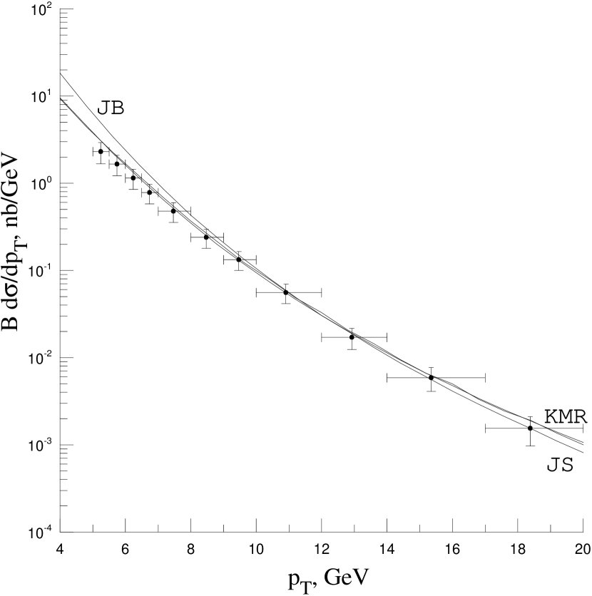
Figure 4: Contributions to the $p_{T}$ distribution of $J/\psi$ mesons from $\chi_{cJ}$ decays in hadroproduction in $p\overline{p}$ scattering with $\sqrt{S}=1.8$ TeV and $|y|<0.6$ from the sum of the partonic subprocesses $R+R\rightarrow\chi_{cJ}[^{3}P_{J}^{(1)}]$ and $R+R\rightarrow\chi_{cJ}[^{3}S_{1}^{(8)}]$, the latter of which being quite unimportant, compared with CDF data from Tevatron run I CDFI . The theoretical results are obtained with the JB JB , JS JS , or KMR KMR unintegrated gluon distribution functions. The decay branching fraction $B(J/\psi\to\mu^{+}+\mu^{-})$ is included.

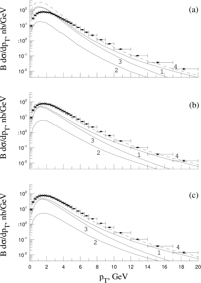
Figure 5: Contributions to the $p_{T}$ distribution of prompt $J/\psi$ hadroproduction in $p\overline{p}$ scattering with $\sqrt{S}=1.96$ TeV and $|y|<0.6$ from (1) direct production, (2) $\psi^{\prime}$ decays, (3) $\chi_{cJ}$ decays, and (4) their sum compared with CDF data from Tevatron run II CDFII . The theoretical results are obtained with the (a) JB JB , (b) JS JS , or (c) KMR KMR unintegrated gluon distribution functions. The decay branching fraction $B(J/\psi\to\mu^{+}+\mu^{-})$ is included.

In Figs. 2–5, we compare the CDF data on $J/\psi$ mesons from direct production, $\psi^{\prime}$ decays, and $\chi_{cJ}$ decays in run I CDFI and from prompt production in run II CDFII , respectively, with the theoretical results evaluated with the NMEs listed in Table 1. From Fig. 2, we observe that the color-singlet contribution is significant, especially at low values of $p_{T}$, and comparable to the one from the ${}^{1}S_{0}^{(8)}$ channel. As is familiar from the collinear parton model, the ${}^{3}S_{1}^{(8)}$ contribution makes up the bulk of the cross section at large values of $p_{T}$. Incidentally, the values of $\langle{\cal O}^{J/\psi}[^{3}S_{1}^{(8)}]\rangle$ obtained in the $k_{T}$-factorization framework are in average quite close to the one obtained in the collinear parton model, as may be seen from Table 1. The situation is very similar for $J/\psi$ production from $\psi^{\prime}$ decay, considered in Fig. 3, except that the ${}^{1}S_{0}^{(8)}$ and ${}^{3}P_{J}^{(8)}$ contributions are negligible.

At this point, we wish to compare our results for direct $J/\psi$ hadroproduction in the $k_{T}$-factorization approach with the literature, specifically with Refs. CDFBaranov ; KTYuan , which consider the partonic subprocess (20). By contrast, in Ref. KTTeryaev , the NLO subprocess $R+R\to J/\psi[{{}^{3}}S_{1}^{(8)}]+g$ was studied, leaving aside the LO subprocess (20). In Ref. KTYuan , the value $\langle{\cal O}^{J/\psi}[{}^{3}S_{1}^{(8)}]\rangle=7.0\times 10^{-3}$ GeV³ was obtained using the Kwiecinski-Martin-Stasto (KMS) KMS unintegrated gluon distribution function. This value is 2.6 times larger than the result we found using the KMR KMR version, which is very similar to the KMS one. We attribute this difference in $\langle{\cal O}^{J/\psi}[{}^{3}S_{1}^{(8)}]\rangle$ to the different scale choice, $\mu=k_{T}$, used by the authors of Ref. KTYuan . Adopting their value for $\langle{\cal O}^{J/\psi}[{}^{3}S_{1}^{(8)}]\rangle$, we can reproduce their result for the respective cross section contribution. On the other hand, the value $\langle{\cal O}^{J/\psi}[{}^{3}S_{1}^{(8)}]\rangle=15.0\times 10^{-3}$ GeV³ found in Ref. CDFBaranov exceeds the one of Ref. KTYuan by a factor of 2.1 and our KMR value by a factor of 5.6. Furthermore, the cross section evaluated in Ref. CDFBaranov falls off with $p_{T}$ considerably more slowly than in Ref. KTYuan and here, only by one order of magnitude as $p_{T}$ runs from 2 to 20 GeV, while the unintegrated gluon density in the proton falls off with $k_{T}$ far more rapidly.

The discussion of $J/\psi$ production from radiative $\chi_{cJ}$ decays, considered in Fig. 4, is simpler because there is only one free parameter in the fit, namely $\langle{\cal O}^{\chi_{c0}}[{{}^{3}}S_{1}^{(8)}]\rangle$. We confirm the conclusion of Ref. KTTeryaev , that, in the $k_{T}$-factorization approach, the color-singlet contribution is sufficient to describe the data. In fact, the best fit is realized when $\langle{\cal O}^{\chi_{c0}}[{{}^{3}}S_{1}^{(8)}]\rangle$ is taken to be zero or very small. In case of the JB gluon density, the fitting procedure even favors a negative value of $\langle{\cal O}^{\chi_{c0}}[{{}^{3}}S_{1}^{(8)}]\rangle$.

In Fig. 5, the $p_{T}$ distribution of prompt $J/\psi$ production in run II is broken down into the contributions from direct production, $\psi^{\prime}$ decays, and $\chi_{cJ}$ decays. We observe that the latter is dominant for $p_{T}\lesssim 5$ GeV, while prompt $J/\psi$ mesons are preferably produced directly at larger values of $p_{T}$. The contribution from $\psi^{\prime}$ decays stays at the level of several percent for all values of $p_{T}$. While the JS JS and KMR KMR gluon densities allow for a faithful description of the measured $p_{T}$ distribution CDFII , the JB JB one has a problem in the low-$p_{T}$ range, at $p_{T}\lesssim 5$ GeV, where even the $\chi_{cJ}$-decay contribution, which is entirely of color-singlet origin, exceeds the data. This problem can be traced to the speed of growth of the JB gluon density as $k_{T}\to 0$. By contrast, the JS and KMR gluon densities are smaller and approximately $k_{T}$ independent at low values of $k_{T}$. For this reason, we excluded the CDF prompt-$J/\psi$ data from run I CDFI and run II CDFII from our fit based on the JB gluon density.

Considering the color-octet NMEs relevant for the $J/\psi$, $\psi^{\prime}$ and $\chi_{cJ}$ production mechanisms, we can formulate the following heuristic rule for favoured transitions from color-octet to color-singlet states: $\Delta L\simeq 0$ and $\Delta S\simeq 0$; i.e. these transitions are doubly chromoelectric and preserve the orbital angular momentum and the spin of the heavy-quark bound state.

VI Charmonium production at HERA

At HERA, the cross section of prompt $J/\psi$ production was measured in a wide range of the kinematic variables $W^{2}=(P+q)^{2}$, $Q^{2}=-q^{2}$, $y_{2}=(P\cdot q)/(P\cdot k)$, $z=(P\cdot p)/(P\cdot q)$, $p_{T}$ and $y$, where $P^{\mu}$, $k^{\mu}$, $k^{\prime\mu}$, $q^{\mu}=k^{\mu}-k^{\prime\mu}$, and $p^{\mu}$ are the four-momenta of the incoming proton, incoming lepton, scattered lepton, virtual photon, and produced $J/\psi$ meson, respectively, both in photoproduction epZEUS , at small values of $Q^{2}$, and deep-inelastic scattering (DIS) epH1 , at large values of $Q^{2}$. At sufficiently large values of $Q^{2}$, the virtual photon behaves like a point-like object, while, at low values of $Q^{2}$, it can either act as a point-like object (direct photoproduction) or interact via its quark and gluon content (resolved photoproduction). Resolved photoproduction is only important at low values of $z$.

In the region $z\lesssim 1$, diffractive production, which is beyond the scope of this paper, takes place. In order to suppress the diffractive-production contribution, one usually applies the acceptance cut $z<0.9$. This effectively eliminates the contributions from the $2\to 1$ partonic subprocesses (22) and (24), so that we are left with the $2\to 2$ partonic subprocesses (23) and (25).

Let us first present the relevant formulas for the double differential cross sections of DIS, direct photoproduction, and resolved photoproduction. In the case of DIS, we have

$$\frac{d\sigma^{\mathrm{KT}}(p+e\to e+{\cal H}+X)}{d|{\bf p}_{T}|^{2}dz}=\frac{1}{8z(2\pi)^{5}}\int{dQ^{2}}\int{dy_{2}}\int{d|{\bf k}_{1T}|^{2}}\int{d\varphi_{1}}\int{d\varphi_{2}}$$

$${}\times\Phi_{p}(x_{1},|{\bf k}_{1T}|^{2},\mu^{2})\frac{\overline{|{\cal A}(R+e\to e+{\cal H}+g)|^{2}}}{(y_{2}-\chi_{2})(2x_{1}S)^{2}},$$ (52)

where

$$x_{1} = \frac{1}{(y_{2}-\chi_{2})S}\left[({\bf k}_{1T}+{\bf q}_{2T}-{\bf p}_{T})^{2}-M^{2}-|{\bf p}_{T}|^{2}+y_{2}\chi_{1}S+(y_{2}-\chi_{2})Q^{2}\right],$$

$$\chi_{1} = \frac{p^{0}+p^{3}}{2E_{p}},\qquad\chi_{2}=\frac{p^{0}-p^{3}}{2E_{e}}.$$ (53)

Here, $E_{p}$ and $E_{e}$ are the proton and lepton energies in the laboratory frame, and we have $S=4E_{p}E_{e}$ and $|{\bf q}_{2T}|=\sqrt{(1-y_{2})Q^{2}}$.

In the case of direct photoproduction, we have

$$\frac{d\sigma^{\mathrm{KT}}(p+e\to e+{\cal H}+X)}{d|{\bf p}_{T}|^{2}dz}=\frac{1}{2z(2\pi)^{2}}\int{dy_{2}}\int{d|{\bf k}_{1T}|^{2}}\int{d\varphi_{1}}$$ (54)

$${}\times\Phi_{p}(x_{1},|{\bf k}_{1T}|^{2},\mu^{2})f_{\gamma/e}(y_{2})\frac{\overline{|{\cal A}(R+\gamma\to{\cal H}+g)|^{2}}}{y_{2}(y_{2}-\chi_{2})(2x_{1}S)^{2}},$$

where

$$x_{1}=\frac{1}{(y_{2}-\chi_{2})S}\left[({\bf k}_{1T}-{\bf p}_{T})^{2}-M^{2}-|{\bf p}_{T}|^{2}+y_{2}\chi_{1}S\right]$$ (55)

and $f_{\gamma/e}(y_{2})$ is the quasi-real photon flux. In the Weizäcker-Williams approximation, the latter takes the form

$$f_{\gamma/e}(y_{2})=\frac{\alpha}{2\pi}\left[\frac{1+(1-y_{2})^{2}}{y_{2}}\ln\frac{Q_{\rm max}^{2}}{Q_{\rm min}^{2}}+2m_{e}^{2}y_{2}\left(\frac{1}{Q_{\rm min}^{2}}-\frac{1}{Q_{\rm max}^{2}}\right)\right],$$ (56)

where $Q_{\rm min}^{2}=m_{e}^{2}y_{2}^{2}/(1-y_{2})$ and $Q^{2}_{\rm max}$ is determined by the experimental set-up, e.g. $Q^{2}_{\rm max}=1$ GeV² epZEUS .

In the case of resolved photoproduction, we take into account the $2\to 1$ and $2\to 2$ partonic subprocesses (20) and (21), respectively, where the first reggeized gluon comes from the proton and the second one from the photon. For subprocess (20), the relevant doubly differential cross section reads:

$$\frac{d\sigma^{\mathrm{KT}}(p+e\to e+{\cal H}+X)}{d|{\bf p}_{T}|^{2}dz}=\frac{1}{2z(|{\bf p}_{T}|^{2}+M^{2})^{2}}\int{dy_{2}}\int{d|{\bf k}_{1T}|^{2}}\int{d\varphi_{1}}$$ (57)

$$\times\Phi_{p}(x_{1},|{\bf k}_{1T}|^{2},\mu^{2})f_{\gamma/e}(y_{2})\Phi_{\gamma}(x_{2},|{\bf k}_{2T}|^{2},\mu^{2}){\overline{|{\cal A}(R+R\to{\cal H})|^{2}}},$$

where

$$x_{1}=\chi_{1},\quad x_{2}=\frac{\chi_{2}}{y_{2}},\quad{\bf k}_{2T}={\bf p}_{T}-{\bf k}_{1T}.$$ (58)

For subprocess (21), the relevant doubly differential cross section is given by

$$\frac{d\sigma^{\mathrm{KT}}(p+e\to e+{\cal H}+X)}{d|{\bf p}_{T}|^{2}dz}=\frac{1}{2z(1-z)(2\pi)^{3}}\int{dy_{2}}\int{d|{\bf k}_{1T}|^{2}}\int{d\varphi_{1}}\int{dx_{2}}\int{d|{\bf k}_{2T}|^{2}}\int{d\varphi_{2}}$$

$$\times\Phi_{p}(x_{1},|{\bf k}_{1T}|^{2},\mu^{2})f_{\gamma/e}(y_{2})\Phi_{\gamma}(x_{2},|{\bf k}_{2T}|^{2},\mu^{2})\frac{\overline{|{\cal A}(R+R\to{\cal H}+g)|^{2}}}{x_{2}(2x_{1}x_{2}y_{2}S)^{2}},$$ (59)

where

$$x_{1} = \frac{1}{(x_{2}y_{2}-\chi_{2})S}\left[({\bf k}_{1T}-{\bf p}_{T})^{2}-M^{2}-|{\bf p}_{T}|^{2}+x_{2}y_{2}\chi_{1}S\right].$$ (60)

To evaluate the unintegrated gluon distribution function in the resolved photon, $\Phi_{\gamma}(x_{2},|{\bf k}_{2T}|^{2},\mu^{2})$, we use a procedure suggested by Blümlein JBPhoton , which is similar to the proton case JB . As input for this, we use the collinear parton distribution functions of the resolved photon by Glück, Reya, and Vogt (GRV_γ) GRVPhoton .

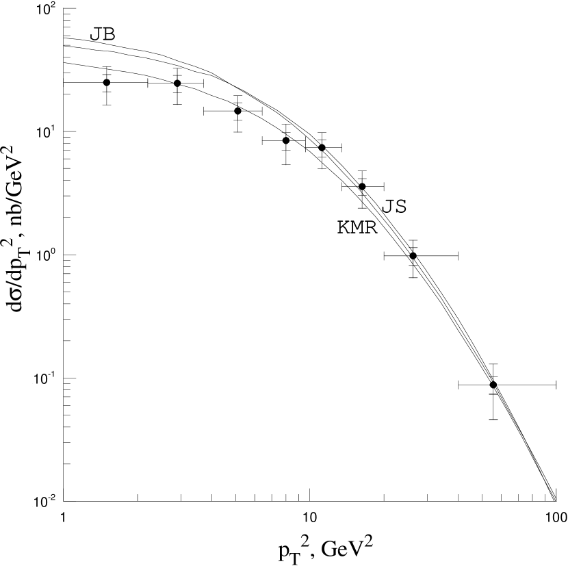
Figure 8: Contribution to the $p_{T}^{2}$ distribution of prompt $J/\psi$ electroproduction in $ep$ scattering with $E_{p}=920$ GeV, $E_{e}=27.5$ GeV, 50 GeV${}<W<225$ GeV, 2 GeV${}^{2}<Q^{2}<100$ GeV², and $0.3<z<0.9$ from the color-singlet subprocess $R+e\rightarrow e+{\cal H}[^{3}S_{1}^{(1)}]+g$ compared with H1 data from HERA epH1 . The theoretical results are obtained with the JB JB , JS JS , or KMR KMR unintegrated gluon distribution functions.

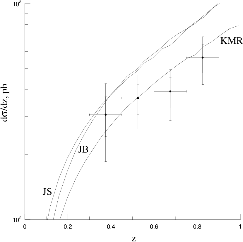
Figure 9: Contribution to the $z$ distribution of prompt $J/\psi$ electroproduction in $ep$ scattering with $E_{p}=920$ GeV, $E_{e}=27.5$ GeV, 50 GeV${}<W<225$ GeV, 2 GeV${}^{2}<Q^{2}<100$ GeV², and $p_{T}>1$ GeV from the color-singlet subprocess $R+e\rightarrow e+{\cal H}[^{3}S_{1}^{(1)}]+g$ compared with H1 data from HERA epH1 . The theoretical results are obtained with the JB JB , JS JS , or KMR KMR unintegrated gluon distribution functions.

In Figs. 6–9, our NRQCD predictions in the $k_{T}$-factorization approach, evaluated with the NMEs from Table 1, are compared with the HERA data epZEUS ; epH1 . Specifically, Figs. 6 and 7 refer to the $p_{T}^{2}$ and $z$ distributions in photoproduction with $E_{p}=820$ GeV, $E_{e}=27.5$ GeV, 60 GeV${}<W<240$ GeV, and $Q^{2}<1$ GeV² epZEUS , while Figs. 8 and 9 refer to those in DIS with $E_{p}=920$ GeV, $E_{e}=27.5$ GeV, 50 GeV${}<W<225$ GeV, and 2 GeV${}^{2}<Q^{2}<100$ GeV² epH1 . Acceptance cuts common to both photoproduction and DIS include $p_{T}>1$ GeV and $0.3<z<0.9$. In this regime, the LO NRQCD predictions in the $k_{T}$-factorization approach are mainly due to the color-singlet channels and are thus fairly independent of the color-octet NMEs presented in Table 1. Therefore, our results agree well with previous calculations in the CSM SaleevZotov94 , up to minor differences in the choice of the color-singlet NMEs and the $c$-quark mass.

VII Charmonium production at LEP2

Some time ago, the DELPHI Collaboration presented data on the inclusive cross section of $J/\psi$ photoproduction in $\gamma\gamma$ collisions ($e^{+}+e^{-}\to e^{+}+e^{-}+J/\psi+X$) at LEP2, taken as a function of the $J/\psi$ transverse momentum $p_{T}$ LEPJpsi . The $J/\psi$ mesons were identified through their decays to $\mu^{+}\mu^{-}$ pairs, and events where the system $X$ contains a prompt photon were suppressed by requiring that at least four charged tracks were reconstructed. The average $e^{+}e^{-}$ center-of-mass energy was $\sqrt{S}=197$ GeV, the scattered positrons and electrons were antitagged, with maximum angle $\theta_{\rm max}=32$ mrad, and the maximum $\gamma\gamma$ center-of-mass energy was chosen to be $W=35$ GeV in order to reject the major part of the non-two-photon events.

Under LEP2 experimental conditions, most $J/\psi$ mesons are produced promptly, while the cross section for $J/\psi$ mesons from $b$-hadron decays is estimated to be about 1% of the total $J/\psi$ cross section KniehlLEP and can be safely neglected. Because the average value of the photon virtuality $Q^{2}$ is small, the Weizsäcker-Williams approximation can be used to evaluate the $e^{+}e^{-}$ cross section from the $\gamma\gamma$ cross section as

$$d\sigma(e^{+}+e^{-}\to e^{+}+e^{-}+{\cal H}+X)=\int dy_{1}\int dy_{2}\,f_{\gamma/e}(y_{1})f_{\gamma/e}(y_{2})d\sigma(\gamma+\gamma\to{\cal H}+X).$$ (61)

The process $e^{+}+e^{-}\to e^{+}+e^{-}+J/\psi+X$ receives contributions from direct, single-resolved, and double-resolved photoproduction. The relevant partonic subprocesses are: $\gamma+\gamma\to{\cal H}[{{}^{3}S}_{1}^{(8)}]+g$, $\gamma+R\to{\cal H}[{{}^{1}S}_{0}^{(8)},{{}^{3}P}_{J}^{(8)}]$, $\gamma+R\to{\cal H}[{{}^{3}S}_{1}^{(1)}]+g$, $R+R\to{\cal H}[{{}^{3}S}_{1}^{(8)},{{}^{1}S}_{0}^{(8)},{{}^{3}P}_{J}^{(8)}]$, and $R+R\to{\cal H}[{{}^{3}S}_{1}^{(1)}]+g$. The squared amplitude of $\gamma+\gamma\to{\cal H}[^{3}S_{1}^{(8)}]+g$ may be found in Ref. KniehlLEP , the ones for the other partonic subprocesses were presented in Sec. IV.

The cross section of direct photoproduction is evaluated as

$$\frac{d\sigma(e^{+}+e^{-}\to e^{+}+e^{-}+{\cal H}+X)}{d|{\bf p}_{T}|^{2}dy}=\frac{1}{4\pi}\int{dy_{2}}\,f_{\gamma/e}(y_{1})f_{\gamma/e}(y_{2})$$

$${}\times\frac{y_{1}y_{2}}{y_{2}-\xi_{2}}\,\frac{\overline{|{\cal A}(\gamma+\gamma\to{\cal H}+g)|^{2}}}{(2y_{1}y_{2}S)^{2}},$$ (62)

where $\xi_{1}$ and $\xi_{2}$ are defined in Eq. (48) and

$$y_{1}=\frac{y_{2}\xi_{1}S-M^{2}}{(y_{2}-\xi_{2})S}.$$ (63)

In the case of single-resolved photoproduction via the $2\to 1$ subprocesses, we have

$$\frac{d\sigma^{\mathrm{KT}}(e^{+}+e^{-}\to e^{+}+e^{-}+{\cal H}+X)}{d|{\bf p}_{T}|^{2}dy}=4\pi\int{dy_{1}}\,f_{\gamma/e}(y_{1})f_{\gamma/e}(y_{2})$$

$$\times\Phi_{\gamma}(x_{1},|{\bf k}_{1T}|^{2},\mu^{2})y_{2}\frac{\overline{|{\cal A}(R+\gamma\to{\cal H})|^{2}}}{(2x_{1}y_{1}y_{2}S)^{2}},$$ (64)

where $x_{1}=\xi_{1}/y_{1}$, $y_{2}=\xi_{2}$, and ${\bf k}_{1T}={\bf p}_{T}$. In the case of single-resolved photoproduction via the $2\to 2$ subprocess, we have

$$\frac{d\sigma^{\mathrm{KT}}(e^{+}+e^{-}\to e^{+}+e^{-}+{\cal H}+X)}{d|{\bf p}_{T}|^{2}dy}=\frac{1}{2(2\pi)^{2}}\int{dy_{1}}\int{dy_{2}}\int{d|{\bf k}_{1T}|^{2}}\int{d\varphi_{1}}\,f_{\gamma/e}(y_{1})f_{\gamma/e}(y_{2})$$

$${}\times\Phi_{\gamma}(x_{1},|{\bf k}_{1T}|^{2},\mu^{2})\frac{y_{2}}{y_{2}-\xi_{2}}\,\frac{\overline{|{\cal A}(R+\gamma\to{\cal H}+g)|^{2}}}{(2x_{1}y_{1}y_{2}S)^{2}},$$ (65)

where

$$x_{1}=\frac{1}{y_{1}(y_{2}-\xi_{2})S}\left[({\bf k}_{1T}-{\bf p}_{T})^{2}-M^{2}-|{\bf p}_{T}|^{2}+y_{2}\xi_{1}S\right].$$ (66)

In the case of double-resolved photoproduction via the $2\to 1$ subprocesses, we have

$$\frac{d\sigma^{\mathrm{KT}}(e^{+}+e^{-}\to e^{+}+e^{-}+{\cal H}+X)}{d|{\bf p}_{T}|^{2}dy}=2\int{dy_{1}}\int{dy_{2}}\int{d|{\bf k}_{1T}|^{2}}\int{d\varphi_{1}}\,f_{\gamma/e}(y_{1})f_{\gamma/e}(y_{2})$$

$${}\times\Phi_{\gamma}(x_{1},|{\bf k}_{1T}|^{2},\mu^{2})\Phi_{\gamma}(x_{2},|{\bf k}_{2T}|^{2},\mu^{2})\frac{\overline{|{\cal A}(R+R\to{\cal H})|^{2}}}{(2x_{1}x_{2}y_{1}y_{2}S)^{2}},$$ (67)

where $x_{1}=\xi_{1}/y_{1}$, $x_{2}=\xi_{2}/y_{2}$, and ${\bf k}_{2T}={\bf p}_{T}-{\bf k}_{1T}$. In the case of double-resolved photoproduction via the $2\to 2$ subprocess, we have

$$\frac{d\sigma^{\mathrm{KT}}(e^{+}+e^{-}\to e^{+}+e^{-}+{\cal H}+X)}{d|{\bf p}_{T}|^{2}dy}=\frac{1}{2(2\pi)^{3}}\int{dy_{1}}\int{dy_{2}}\int{d|{\bf k}_{1T}|^{2}}\int{d\varphi_{1}}$$

$$\times\int{dx_{2}}\int{d|{\bf k}_{2T}|^{2}}\int{d\varphi_{2}}\,f_{\gamma/e}(y_{1})\Phi_{\gamma}(x_{1},|{\bf k}_{1T}|^{2},\mu^{2})f_{\gamma/e}(y_{2})\Phi_{\gamma}(x_{2},|{\bf k}_{2T}|^{2},\mu^{2})$$

$$\times\frac{y_{2}}{x_{2}y_{2}-\xi_{2}}\,\frac{\overline{|{\cal A}(R+R\to{\cal H}+g)|^{2}}}{(2x_{1}x_{2}y_{1}y_{2}S)^{2}},$$ (68)

where

$$x_{1}=\frac{1}{y_{1}(x_{2}y_{2}-\xi_{2})S}\left[({\bf k}_{1T}+{\bf k}_{2T}-{\bf p}_{T})^{2}-M^{2}-|{\bf p}_{T}|^{2}+x_{2}y_{2}\xi_{1}S\right].$$ (69)

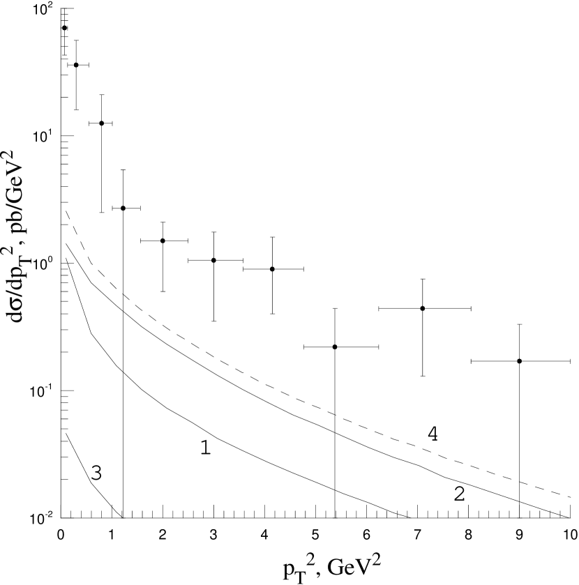
Figure 10: Contributions to the $p_{T}^{2}$ distribution of prompt $J/\psi$ photoproduction in $e^{+}e^{-}$ annihilation with $\sqrt{S}=197$ GeV, $Q^{2}<9.93$ GeV², $W<35$ GeV, and $|y|<2$ from the partonic subprocesses (1) $R+\gamma\rightarrow{\cal H}[{{}^{1}S}_{0}^{(8)},{{}^{3}P}_{J}^{(8)}]$, (2) $R+\gamma\rightarrow{\cal H}[^{3}S_{1}^{(1)}]+g$, (3) $\gamma+\gamma\rightarrow{\cal H}[^{3}S_{1}^{(8)}]+g$, $R+R\to{\cal H}[{{}^{3}S}_{1}^{(8)},{{}^{1}S}_{0}^{(8)},{{}^{3}P}_{J}^{(8)}]$, and $R+R\to{\cal H}[{{}^{3}S}_{1}^{(1)}]+g$, and (4) their sum compared with DELPHI data from LEP2 LEPJpsi . The theoretical results are obtained with the JB JB unintegrated gluon distribution function.

In Fig. 10, we confront the $p_{T}^{2}$ distribution of $e^{+}+e^{-}\to e^{+}+e^{-}+J/\psi+X$, where $X$ is devoid of prompt photons, measured by DELPHI LEPJpsi with our full theoretical prediction (line No. 4), which is broken down into the single-resolved color-octet contribution (line No. 1), the single-resolved color-singlet contribution (line No. 2), and the direct plus double-resolved contributions (line No. 3). We observe that the single-resolved contribution makes up the bulk of the cross section, while the direct and double-resolved contributions are greatly suppressed, and that, within the single-resolved contribution, the color-singlet channel is dominant. The experimental data overshoot the theoretical prediction by a moderate factor of 2–3. For the case of $\gamma\gamma$ collisions, we conclude that the color-singlet processes are dominant in the $k_{T}$-factorization approach, a situation familiar from photo- and electroproduction in $ep$ collisions considered in Sec. VI. The situation is quite different for the collinear parton model, where color-octet processes dominate KniehlLEP .

Recently, in Ref. ZotovLEP , it was attempted to interpret the DELPHI data in the $k_{T}$-factorization approach invoking only the CSM and neglecting the cascade decays of the $\psi^{\prime}$ and $\chi_{cJ}$ mesons. Curve No. 2 in Fig. 10 approximately agrees with the corresponding predictions in Ref. ZotovLEP for $m_{c}=1.55$ GeV. In Ref. ZotovLEP , a significantly lower value of $m_{c}$ is employed to reach agreement with the DELPHI data.

VIII Conclusion

Working at LO in the $k_{T}$-factorization approach to NRQCD, we analytically evaluated the squared amplitudes of prompt charmonium production by reggeized gluons in $RR$, $R\gamma$, and $Re$ collisions. We extracted the relevant color-octet NMEs, $\langle{\cal O}^{\cal H}[^{3}S_{1}^{(8)}]\rangle$, $\langle{\cal O}^{\cal H}[^{1}S_{0}^{(8)}]\rangle$, and $\langle{\cal O}^{\cal H}[^{3}P_{0}^{(8)}]\rangle$ for ${\cal H}=J/\psi$, $\psi^{\prime}$, and $\chi_{cJ}$ through fits to $p_{T}$ distributions measured by the CDF Collaboration in $p\bar{p}$ collisions at the Tevatron with $\sqrt{S}=1.8$ TeV CDFI and 1.96 TeV CDFII using three different versions of unintegrated gluon distribution function, namely JB JB , JS JS , and KMR KMR . Appealing to the assumed NRQCD factorization, we used the NMEs thus obtained to predict various cross section distributions of prompt $J/\psi$ photoproduction and electroproduction in $ep$ collisions and photoproduction in $e^{+}e^{-}$ collisions and compared them with ZEUS epZEUS and H1 epH1 data from HERA and DELPHI LEPJpsi data from LEP2, respectively. In the case of photoproduction, we included both the direct and resolved contributions. As for the unintegrated parton distribution functions of the proton and the resolved photon, we assumed the gluon content to be dominant.

Our fits to the Tevatron data turned out to be satisfactory, except for the one to the $\chi_{cJ}$ sample based on the JB gluon density in the proton, where the fit result significantly exceeded the measured cross section in the small-$p_{T}$ region. We found agreement with the HERA and LEP2 data within a factor of 2, which is the typical size of the theoretical uncertainty due to the lack of knowledge of the precise value of the $c$-quark mass and the NLO corrections. Specifically, we found that direct and resolved photoproduction in $ep$ collisions under HERA kinematic conditions dominantly proceed through color-singlet processes, namely $R(p)+\gamma\to{\cal H}[{{}^{3}}S_{1}^{(1)}]+g$ and $R(p)+R(\gamma)\to{\cal H}[{{}^{3}}S_{1}^{(1)}]+g$, respectively. Similarly, photoproduction in $e^{+}e^{-}$ collisions under LEP2 kinematic conditions is mainly mediated via the color-singlet subprocess $R(\gamma)+\gamma\to{\cal H}[{{}^{3}}S_{1}^{(1)}]+g$, but the color-octet subprocess $R(\gamma)+\gamma\to{\cal H}[{{}^{1}}S_{0}^{(8)}]$ also contributes appreciably.

LO predictions in both the collinear parton model and the $k_{T}$-factorization framework suffer from sizeable theoretical uncertainties, which are largely due to unphysical-scale dependences. Substantial improvement can only be achieved by performing full NLO analyses. While the stage for the NLO NRQCD treatment of $2\to 2$ processes has been set in the collinear parton model kkms , conceptual issues still remain to be clarified in the $k_{T}$-factorization approach. Since, at NLO, incoming partons can gain a finite $k_{T}$ kick through the perturbative emission of partons, one expects that essential features produced by the $k_{T}$-factorization approach at LO will thus automatically show up at NLO in the collinear parton model.

Figure 1: Contributions to the $p_{T}$ distribution of prompt $J/\psi$ hadroproduction in $p\overline{p}$ scattering with $\sqrt{S}=1.96$ TeV and $|y|<0.6$ from the relevant color-octet states compared with CDF data from Tevatron run II CDFII . All distributions are normalized to unity at their peaks.

Figure 2: Contributions to the $p_{T}$ distribution of direct $J/\psi$ hadroproduction in $p\overline{p}$ scattering with $\sqrt{S}=1.8$ TeV and $|y|<0.6$ from the partonic subprocesses (1) $R+R\rightarrow J/\psi[^{3}S_{1}^{(8)}]$, (2) $R+R\rightarrow J/\psi[^{1}S_{0}^{(8)},^{3}P_{J}^{(8)}]$, (3) $R+R\rightarrow J/\psi[^{3}S_{1}^{(1)}]+g$, and (4) their sum compared with CDF data from Tevatron run I CDFI . The theoretical results are obtained with the (a) JB JB , (b) JS JS , or (c) KMR KMR unintegrated gluon distribution functions. The decay branching fraction $B(J/\psi\to\mu^{+}+\mu^{-})$ is included.

Figure 3: Contributions to the $p_{T}$ distribution of $J/\psi$ mesons from $\psi^{\prime}$ decays in hadroproduction in $p\overline{p}$ scattering with $\sqrt{S}=1.8$ TeV and $|y|<0.6$ from the partonic subprocesses (1) $R+R\rightarrow\psi^{\prime}[{{}^{3}S}_{1}^{(8)}]$, (2) $R+R\rightarrow\psi^{\prime}[{{}^{1}S}_{0}^{(8)},{{}^{3}P}_{J}^{(8)}]$ (this contribution actually vanished), (3) $R+R\rightarrow\psi^{\prime}[{{}^{3}S}_{1}^{(1)}]+g$, and (4) their sum compared with CDF data from Tevatron run I CDFI . The theoretical results are obtained with the (a) JB JB , (b) JS JS , or (c) KMR KMR unintegrated gluon distribution functions. The decay branching fraction $B(J/\psi\to\mu^{+}+\mu^{-})$ is included.

Figure 6: Contribution to the $p_{T}^{2}$ distribution of prompt $J/\psi$ photoproduction in $ep$ scattering with $E_{p}=820$ GeV, $E_{e}=27.5$ GeV, $60$ GeV${}<W<240$ GeV, $Q^{2}<1$ GeV², and $0.3<z<0.9$ from the direct-photon subprocess $R+\gamma\rightarrow{\cal H}[^{3}S_{1}^{(1)}]+g$ compared with ZEUS data from HERA epZEUS . The resolved-photon subprocesses $R+R\rightarrow{\cal H}[^{3}S_{1}^{(1)},^{3}P_{J}^{(1)},^{3}S_{1}^{(8)},^{1}S_{0}^{(8)},^{3}P_{J}^{(8)}]$ are neglected. The theoretical results are obtained with the JB JB , JS JS , or KMR KMR unintegrated gluon distribution functions.

Figure 7: Contributions to the $z$ distribution of prompt $J/\psi$ photoproduction in $ep$ scattering with $E_{p}=820$ GeV, $E_{e}=27.5$ GeV, 60 GeV${}<W<240$ GeV, $Q^{2}<1$ GeV², and (a) $p_{T}>1$ GeV, (b) $p_{T}>2$ GeV, or (c) $p_{T}>3$ GeV from (1) the direct-photon subprocess $R+\gamma\rightarrow{\cal H}[^{3}S_{1}^{(1)}]+g$, (2) the resolved-photon subprocesses $R+R\rightarrow{\cal H}[^{3}S_{1}^{(1)},^{3}P_{J}^{(1)},^{3}S_{1}^{(8)},^{1}S_{0}^{(8)},^{3}P_{J}^{(8)}]$, and (3) their sum compared with ZEUS data from HERA epZEUS . The theoretical results are obtained with the JB JB unintegrated gluon distribution function.

Table 1: NMEs for $J/\psi$, $\psi^{\prime}$, and $\chi_{cJ}$ mesons from fits in the collinear parton model (PM) BKLee using the MRST98LO parton distribution functions of the proton MRST and in the $k_{T}$-factorization approach using the JB JB , JS JS , and KMR KMR unintegrated gluon distribution functions. The CDF prompt data from run I CDFI and run II CDFII have been excluded from our fit based on the JB gluon density.

NME	PM BKLee	Fit JB	Fit JS	Fit KMR
$\langle{\cal O}^{J/\psi}[^{3}S_{1}^{(1)}]\rangle/$GeV3	1.3	1.3	1.3	1.3
$\langle{\cal O}^{J/\psi}[^{3}S_{1}^{(8)}]\rangle/$GeV3	$4.4\times 10^{-3}$	$1.5\times 10^{-3}$	$6.1\times 10^{-3}$	$2.7\times 10^{-3}$
$\langle{\cal O}^{J/\psi}[^{1}S_{0}^{(8)}]\rangle/$GeV3	—	$6.6\times 10^{-3}$	$9.0\times 10^{-3}$	$1.4\times 10^{-2}$
$\langle{\cal O}^{J/\psi}[^{3}P_{0}^{(8)}]\rangle/$GeV5	—	0	0	0
$M_{3.4}^{J/\psi}/$GeV3	$8.7\times 10^{-2}$	$6.6\times 10^{-3}$	$9.0\times 10^{-3}$	$1.4\times 10^{-2}$
$\langle{\cal O}^{\psi^{\prime}}[^{3}S_{1}^{(1)}]\rangle/$GeV3	$6.5\times 10^{-1}$	$6.5\times 10^{-1}$	$6.5\times 10^{-1}$	$6.5\times 10^{-1}$
$\langle{\cal O}^{\psi^{\prime}}[^{3}S_{1}^{(8)}]\rangle/$GeV3	$4.2\times 10^{-3}$	$3.0\times 10^{-4}$	$1.5\times 10^{-3}$	$8.3\times 10^{-4}$
$\langle{\cal O}^{\psi^{\prime}}[^{1}S_{0}^{(8)}]\rangle/$GeV3	—	0	0	0
$\langle{\cal O}^{\psi^{\prime}}[^{3}P_{0}^{(8)}]\rangle/$GeV5	—	0	0	0
$M_{3.5}^{\psi^{\prime}}/$GeV3	$1.3\times 10^{-2}$	0	0	0
$\langle{\cal O}^{\chi_{c0}}[^{3}P_{0}^{(1)}]\rangle/$GeV5	$8.9\times 10^{-2}$	$8.9\times 10^{-2}$	$8.9\times 10^{-2}$	$8.9\times 10^{-2}$
$\langle{\cal O}^{\chi_{c0}}[^{3}S_{1}^{(8)}]\rangle/$GeV3	$2.3\times 10^{-3}$	0	$2.2\times 10^{-4}$	$4.7\times 10^{-5}$
$\chi^{2}/\mathrm{d.o.f}$	—	2.2	4.1	3.0