$J/\psi$, $\psi^{\prime}$ AND $\Upsilon$ PRODUCTION AT HADRON COLLIDERS:
A REVIEW

Abstract

We give an overview of the present status of knowledge of the production of $J/\psi$, $\psi^{\prime}$ and $\Upsilon$ in high-energy hadron collisions. We first present two early models, namely the Colour-Singlet Model (CSM) and the Colour-Evaporation Model (CEM). The first is the natural application of pQCD to quarkonium production and has been shown to fail dramatically to describe experimental data, the second is its phenomenological counterpart and was introduced in the spirit of the quark-hadron duality in the late seventies. Then, we expose the most recent experimental measurements of $J/\psi$, $\psi^{\prime}$ and $\Upsilon$ prompt and direct production at nonzero $p_{T}$ from two high-energy hadron colliders, the Tevatron and RHIC. In a third part, we review six contemporary models describing $J/\psi$, $\psi^{\prime}$ and $\Upsilon$ production at nonzero $p_{T}$.

PACS numbers: 14.40.Gx 13.85.Ni

1 History: from a revolution to an anomaly

1.1 $J/\psi$ and the November revolution

The era of quarkonia has started at the simultaneous discovery of the $J/\psi$ in November 1974 by Ting et al.[1] at BNL and by Richter et al.[2] at SLAC. Richter’s experiment used the electron-positron storage ring SPEAR, whose center-of-momentum energy could be tuned at the desired value. With the Mark I detector, they discovered a sharp enhancement of the production cross section in different channels: $e^{+}e^{-}$, $\mu^{+}\mu^{-}$, $\pi^{+}\pi^{-}$,…On the other hand, Ting’s experiment was based on the high-intensity proton beams of the Alternating Gradient Synchrotron (AGS) working at the energy of 30 GeV, which bombarded a fixed target with the consequence of producing showers of particles detectable by the appropriate apparatus.

In the following weeks, the Frascati group (Bacci et al.[3]) confirmed the presence of this new particle whose mass was approximately 3.1 GeV. The confirmation was so fast that it was actually published in the same issue of Physical Review Letters, ie. vol. 33, no. 23, issued the second of December 1974. In the meantime, Richter’s group discovered another resonant state with a slightly higher mass, which was called $\psi^{\prime}$.

It was also promptly established that the quantum numbers of the $J/\psi$ were the same as those of the photon , i.e. $1^{--}$. Moreover, since the following ratio

$$\begin{split}R=\frac{\hbox{cross section for $e^{+}e^{-}\to$ hadrons}}{\hbox{cross section for $e^{+}e^{-}\to\mu^{+}\mu^{-}$}}\end{split}$$ (1)

was much larger on-resonance than off, it was then clear that the $J/\psi$ did have direct hadronic decays. The same conclusion held for the $\psi^{\prime}$ as well. The study of multiplicity in pion decays indicated that $\psi$ decays were restricted by $G$-parity conservation, holding only for hadrons. Consequently, $J/\psi$ and $\psi^{\prime}$ were rapidly considered as hadrons of isospin 0 and $G$-parity -1.

Particles with charge conjugation $C$ different from -1 were found later. Indeed, they were only produced by decay of $\psi^{\prime\prime}$ and the detection of the radiated photon during the (electromagnetic) decay was then required. The first to achieve this task and discover a new state was the DASP collaboration[4] based at DESY (Deutsches Elektronen-Synchrotron), Hamburg, working at an $e^{+}e^{-}$ storage ring called DORIS. This new particle, named $P_{c}$, had a mass of approximately 3.5 GeV. At SPEAR, other resonances at 3.415, 3.45 and 3.55 GeV were discovered, the 3.5 GeV state was confirmed. Later, these states were shown to be $C=+1$.

Coming back to the ratio $R$, it is instructive to analyse the implication in the framework of the quark model postulated by Gell-Mann and Zweig in 1963. In 1974 at the London conference, Richter presented[5] the experimental situation as in Fig. 1.

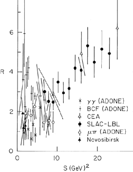
Figure 1: Experimental status of $R$ as of July 1974 (from Ref. Richter:1974vz) .

In the framework of the Gell-Mann-Zweig quark model with three quarks, a plateau was expected with a value of $2/3$ or $2$ if the quark were considered as “coloured” – a new concept introduced recently then –. The sign of a new quark – as the charm quark first proposed by Bjorken and Glashow in 1964[6]– would have been another plateau from a certain energy (roughly its mass) with a height depending on its charge. Retrospectively, one cannot blame anyone for not having seen this “plateau” on this kind of plots. Quoting Richter, “the situation that prevailed in the Summer of 1974” was “vast confusion”.

This charm quark was also required by the mechanism of Glashow, Iliopoulos and Maiani (GIM)[7], in order to cancel the anomaly in weak decays. The charm quark was then expected to exist and to have an electric charge $2/3$. $R$ was therefore to be $10/3$ in the coloured quark model, still not obvious in Fig. 1. This explains why the discovery of such sharp and easily interpreted resonances in November 1974 was a revolution in particle physics.

It became quite rapidly obvious that the $J/\psi$ was the lowest-mass $c\bar{c}$ system with the same quantum numbers as photons – explaining why it was so much produced compared to some other members of its family. These $c\bar{c}$ bound states were named “charmonium”, firstly by Appelquist, De Rújula, Politzer and Glashow[8] in analogy with positronium, whose bound-state level structure was similar.

At that time, the charm had nevertheless always been found hidden, that is in charm-anti-charm bound states. In order to study these explicitly charmed mesons, named $D$, the investigations were based on the assumption that the $D$ was to decay weakly and preferentially into strange quarks. The weak character of the decay motivated physicists to search for parity-violation signals. The first resonance attributed to $D^{0}$ meson was found in $K^{+}\pi^{+}$ decay by Goldhaber et al.[9] in 1976. A little later, $D^{+}$ and $D^{-}$ were also discovered as well as an excited state, $D^{*}$, with a mass compatible with the decay $\psi^{\prime\prime\prime}\to D^{0}D^{*}$. And, finally, the most conclusive evidence for the discovery of charmed meson was the observation of parity violation in $D$ decays[10]. To complete the picture of the charm family, the first charmed baryon was discovered during the same year[11]. The quarks were not anymore just a way to interpret symmetry in masses and spins of particles, they had acquired an existence.

1.2 The bottomonium family

In the meantime, in 1975, another brand new particle was unmasked at SLAC by Perl et al.[12]. This was the first particle of a third generation of quarks and leptons, the $\tau$, a lepton. Following the standard model, more and more trusted, two other quarks were expected to exist. Their discovery would then be the very proof of the theory that was developed since the sixties. Two names for the fifth quark were already chosen: “beauty” and “bottom”, and in both cases represented by the letter $b$; the sixth quark was as well already christened with the letter $t$ for the suggested names “true” or “top”.

The wait was not long: two years. After a false discovery of a resonance at 6.0 GeV, a new dimuon resonance similar to $J/\psi$ and called $\Upsilon$ was brought to light at Fermilab, thanks to the FNAL proton synchrotron accelerator, by Herb et al.[14], with a mass of 9.0 GeV; as for charmonia, the first radial excited state ($\Upsilon(2S)$) was directly found[15] thereafter. Again, the discovery of a new quarkonium was a decisive step forward towards the comprehension of particle physics.

Various confirmations of these discoveries were not long to come. The $3S$ state was then found[16] at Fermilab as well as an evidence that the $4S$ state was lying above the threshold for the production of $B$ mesons. The latter was confirmed at the Cornell $e^{+}e^{-}$ storage ring with the CLEO detector. The first evidence for $B$ meson and, thus, for unhidden $b$ quark, was also brought by the CLEO collaboration[17] in 1980. One year later, “the first evidence for baryons with naked beauty”(sic) was reported by CERN physicists[18].

Another decade was needed for the discovery of the sixth quark which was definitely christened “top”. Indeed, in 1994, the CDF Collaboration found the first evidence for it at the Tevatron collider at Fermilab[19]. The discovery was published in 1995 both by CDF[20] and D$\emptyset$[21]. Unfortunately, due to its very short lifetime, this quark cannot bind with its antiquark to form the toponium. To conclude this historical prelude, we give the spectra (Figs. 2 & 3) of the $c\bar{c}$ and $b\bar{b}$ systems as well as two tables (Tables 1 & 2) summing up the characteristics of the observed states as of today.

Properties of charmonia (cf. Ref. pdg). Meson $n^{2S+1}L_{J}$ $J^{PC}$ Mass (GeV) $\Gamma_{\mu\mu}$ (keV) $\eta_{c}$ $1\ ^{1}S_{0}$ $0^{-+}$ 2.980 N/A $J/\psi$ $1\ ^{3}S_{1}$ $1^{--}$ 3.097 5.40 $\chi_{c0}$, $\chi_{c1}$, $\chi_{c2}$ $1\ ^{3}P_{0,1,2}$ $0^{++}$,$1^{++}$,$2^{++}$ 3.415,3.511,3.556 N/A $h_{c}$ $1\ ^{1}P_{0}$ $1^{+-}$ 3.523 N/A $\eta_{c}(2S)$ $2\ ^{1}S_{0}$ $0^{-+}$ 3.594 N/A $\psi^{\prime}$ $2\ ^{3}S_{1}$ $1^{--}$ 3.686 2.12

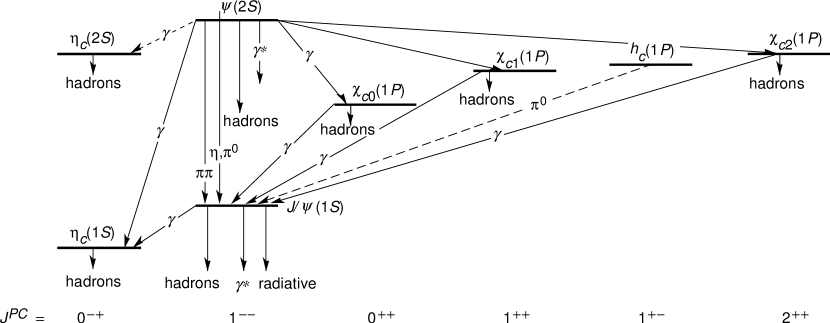
Figure 2: Spectrum and transitions of the charmonium family (Reprinted figure from Ref. pdg with permission of Elsevier. Copyright (2004).).

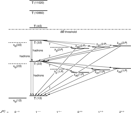
Figure 3: Spectrum and transitions of the bottomonium family (Reprinted figure from Ref. pdg. with permission of Elsevier. Copyright (2004).).

Properties of bottomonia (cf. Ref. pdg) . Meson $n^{2S+1}L_{J}$ $J^{PC}$ Mass (GeV) $\Gamma_{\mu\mu}$ (keV) $\Upsilon(1S)$ $1^{3}S_{1}$ $1^{--}$ 9.460 1.26 $\chi_{b0}$, $\chi_{b1}$ , $\chi_{b2}(1P)$ $1\ ^{3}P_{0,1,2}$ $0^{++}$,$1^{++}$,$2^{++}$ 9.860,9.893,9.913 N/A $\Upsilon(2S)$ $2\ ^{3}S_{1}$ $1^{--}$ 10.023 0.32 $\chi_{b0}$, $\chi_{b1}$, $\chi_{b2}$ (2P) $2\ ^{3}P_{0,1,2}$ $0^{++}$,$1^{++}$,$2^{++}$ 10.232,10.255,10.269 N/A $\Upsilon(3S)$ $3\ ^{3}S_{1}$ $1^{--}$ 10.355 0.48

1.3 Early predictions for quarkonium production

1.3.1 The Colour-Singlet Model

This model is the most natural application of QCD to heavy-quarkonium production in the high-energy regime. It takes its inspiration in the factorisation theorem of QCD[23, 24, 25, 26] where the hard part is calculated by the strict application pQCD and the soft part is factorised in a universal wave function. This model is meant to describe the production not only of $J/\psi$, $\psi(2S)$, $\Upsilon(1S)$, $\Upsilon(2S)$ and $\Upsilon(3S)$, i.e. the ${}^{3}S_{1}$ states, but also the singlet $S$ states $\eta_{c}$ and $\eta_{b}$ as well as the $P$ ($\chi$) and $D$ states.

Its greatest quality resides in its predictive power as the only input, apart from the PDF, namely the wave function, can be determined from data on decay processes or by application of potential models. Nothing more is required. It was first applied to hadron colliders[27, 28, 29], then to electron-proton colliders[30]. The cross sections for ${}^{3}S_{1}$ states were then calculated, as well as also for $\eta$ and $\chi$, for charmonium and for bottomonium. These calculations were compared to ISR and FNAL data from $\sqrt{s}=27$ GeV to $\sqrt{s}=63$ GeV for which the data extended to 6 GeV for the transverse momentum. Updates[31, 32] of the model to describe collisions at the CERN $p\bar{p}$ collider ($\sqrt{s}=630$ GeV) were then presented. At that energy, the possibility that the charmonium be produced from the decay of a beauty hadron was becoming competitive. Predictions for Tevatron energies were also made[32].

In order to introduce the reader to several concepts and quantities that will be useful throughout this Review, let us proceed with a detailed description of this model.

1.3.2 The Model as of early 90’s

It was then based on several approximations or postulates:

• If we decompose the quarkonium production in two steps, first the creation of two on-shell heavy quarks ($Q$ and $\bar{Q}$) and then their binding to make the meson, one postulates the factorisation of these two processes.

• As the scale of the first process is approximately $M^{2}+p_{T}^{2}$, one considers it as a perturbative one. One supposes that its cross section be computable with Feynman-diagram methods.

• As we consider only bound states of heavy quarks (charm and bottom quarks), their velocity in the meson must be small. One therefore supposes that the meson be created with its 2 constituent quarks at rest in the meson frame. This is the static approximation.

• One finally assumes that the colour and the spin of the $Q\bar{Q}$ pair do not change during the binding. Besides, as physical states are colourless, one requires the pair be produced in a colour-singlet state. This explains the name Colour-Singlet Model (CSM).

In high-energy hadronic collisions, the leading contribution comes from a gluon fusion process; as the energy of the collider increases, the initial parton momentum fraction $x_{i}$ needed to produce the quarkonium decreases to reach the region in $x$ where the number of gluons becomes much larger than the number of quarks. One has then only six Feynman diagrams for the ${}^{3}S_{1}$ states production associated with a gluon (see Fig. 4).

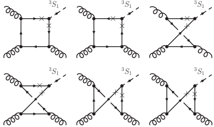
Figure 4: The 6 diagrams for $gg\to\!\!\ ^{3}S_{1}g$ at LO within the CSM.

One usually starts with ${\cal M}(p)$, the perturbative amplitude to produce the heavy-quark pair on-shell with relative momentum $p$ and in a configuration similar to the one of the meson. To realise the latter constraint, one introduces a projection operator; the amplitude ${\cal M}(p)$ is then simply calculated with the usual Feynman rules.

The amplitude to produce the meson is thence given by

$${\cal A}=\int\Phi(\vec{p}){\cal M}(p)\delta(2p^{0})dp,$$ (2)

where $\Phi(\vec{p})$ is the usual Schrödinger wave-function.

Fortunately, one does not have to carry out the integration thanks to the the static approximation which amounts to considering the first non-vanishing term of $\cal A$ when the perturbative part $\cal M$ is expanded in $p$. For $S$-wave, this gives

$$\int\Phi(\vec{p}){\cal M}(p)\delta(2p^{0})dp\simeq\left.{\cal M}\right|_{p=0}\left.\Psi\right|_{\vec{x}=0},$$ (3)

where $\Psi$ is the wave-function in coordinate space, and $\left.\Psi\right|_{\vec{x}=0}$ or $\Psi(0)$ is its value at the origin. For $P$-waves, $\Psi(0)$ is zero, and the second term in the Taylor expansion must be considered; this makes appear $\Psi^{\prime}(0)$. $\Psi(0)$ (or $\Psi^{\prime}(0)$) is the non-perturbative input, which is also present in the leptonic decay width from which it can be extracted.

If the perturbative part ${\cal M}(p)$ is calculated at the leading order in $\alpha_{s}$, this will be referred to as the Leading Order CSM (LO CSM)[27, 28, 29, 30].

1.3.3 The Colour Evaporation Model

This model was initially introduced in 1977[33, 34] and was revived in 1996 by Halzen et al.[35, 36].Contrarily to the CSM, the heavy-quark pair produced by the perturbative interaction is not assumed to be in a colour-singlet state. One simply considers that the colour and the spin of the asymptotic $Q\bar{Q}$ state is randomised by numerous soft interactions occurring after its production, and that, as a consequence, it is not correlated with the quantum numbers of the pair right after its production.

A first outcome of this statement is that the production of a ${}^{3}S_{1}$ state by one gluon is possible, whereas in the CSM it was forbidden solely by colour conservation. In addition, the probability that the $Q\bar{Q}$ pair eventually be in a colour-singlet state is therefore $\frac{1}{9}$, which gives the total cross section to produce a quarkonium:

$$\sigma_{onium}=\frac{1}{9}\int_{2m_{Q}}^{2m_{\bar{q}Q}}dm\frac{d\sigma_{Q\bar{Q}}}{dm}.$$ (4)

This amounts to integrating the cross section of production of $Q\bar{Q}$ from the threshold $2m_{Q}$ up to the threshold to produce two charm or beauty mesons (designated here by $\bar{q}Q$) and one divides by 9 to get the probability of having a colour-singlet state.

The procedure to get the cross section for a definite state, for instance a $J/\psi$, is tantamount to “distributing” the cross sections among all states:

$$\sigma_{J/\psi}=\rho_{J/\psi}\sigma_{onium}.$$ (5)

The natural value for $\rho_{J/\psi}$, as well as for the other states in that approximation, is the inverse of the number of quarkonium lying between $2m_{c}$ and $2m_{D}$. This can be refined by factors arising from spin multiplicity arguments or by the consideration of the mass difference between the produced and the final states. These are included in the Soft-Colour-Interactions approach (SCI) (see section 3.1).

By construction, this model is unable to give information about the polarisation of the quarkonium produced, which is a key test for the other models[37]. Furthermore, nothing but fits can determine the values to input for $\rho$. Considering production ratios for charmonium states within the simplest approach for spin, we should have for instance $\sigma[\eta_{c}]:\sigma[J/\psi]=1:3$ and $\sigma[\chi_{c0}]:\sigma[\chi_{c1}]:\sigma[\chi_{c2}]=1:3:5$, whereas deviations from the predicted ratio for $\chi_{c1}$ and $\chi_{c2}$ have been observed. Moreover, it is unable to describe the observed variation – from one process to another – of the production ratios for charmonium states. For example, the ratio of the cross sections for $\chi_{c}$ and $J/\psi$ differs significantly in photoproduction and hadroproduction, whereas for the CEM these number are strictly constant.

All these arguments make us think that despite its simplicity and its phenomenological reasonable grounds, this model is less reliable than the CSM. It is also instructive to point out that the invocation of reinteractions after the $Q\bar{Q}$ pair production contradicts factorisation, which is albeit required when the PDF are used. However, as we shall see now, the CSM has undergone in the nineties a lashing denial from the data.

1.4 $\psi^{\prime}$ anomaly

In 1984, Halzen et al.[31] noticed that charmonium production from a weak $B$ decay could be significant at high energy – their prediction were made for $\sqrt{s}=540$ GeV – and could even dominate at high enough $p_{T}$. This can be easily understood having in mind that the $B$ meson is produced by fragmentation of a $b$ quark – the latter dresses with a light quark –. And to produce only one $b$ quark at high $p_{T}$ is not so burdensome; the price to pay is only to put one quark propagator off-shell, instead of two for $gg\to\psi g$.

This idea was confirmed by the calculations of Glover et al.[32], which were used as a benchmark by the UA1 Collaboration[38]. After the introduction of a $K$ factor of 2, the measurements agreed with the predictions; however the $p_{T}$ slope was not compatible with $b$-quark fragmentation simulations.

From 1992, the CDF collaboration undertook an analysis of $\psi$ production. They managed to extract unambiguously the prompt component of the signal (not from $B$ decay) using a Silicon Vertex Detector (SVX)[39].

The preliminary results[40] showed an unexpectedly large prompt component. For the $\psi^{\prime}$, the prompt cross section was orders of magnitude above the predictions of the LO CSM (compare the data to the dashed curve on Fig. 5 (right)) . This problem was then referred to as the $\psi^{\prime}$ anomaly. For $J/\psi$, the discrepancy was smaller (Fig. 5 (left)), but it was conceivably blurred by the fact that a significant part of the production was believed to come from $\chi_{c}$ radiative feed-down, but no experimental results were there to confirm this hypothesis.

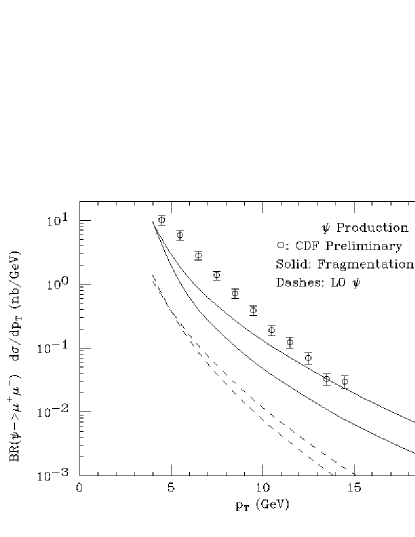
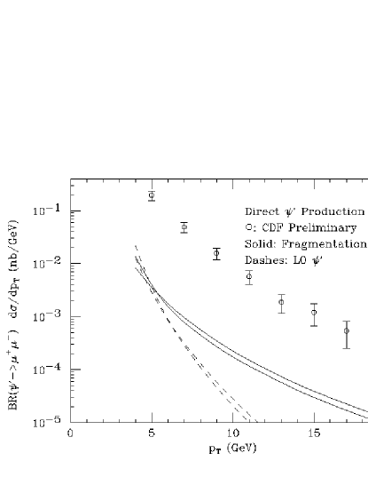
Figure 5: Comparison between preliminary measurements of Ref. :1994dx from CDF and the cross sections obtained by Braaten et al. for LO CSM (dashed curves) of $J/\psi$ (left) and $\psi^{\prime}$ (right), as well as for CSM fragmentation contribution (solid curves). In each case, the two curves depict the extremum values obtained by varying parameters such as $m_{c}$ and the different scales: $\mu_{R}$, $\mu_{F}$, $\mu_{frag}$ (Reprinted figures from Ref. Braaten:1994xb with permission of Elsevier. Copyright (1994).)

1.4.1 Fragmentation within the CSM: the anomaly confirmed

The prediction from the LO CSM for prompt $\psi$ being significantly below these preliminary measurements by CDF, Braaten and Yuan[43] pointed out in 1993 that gluon fragmentation processes, even though of higher order in $\alpha_{s}$, were to prevail over the LO CSM for $S$-wave mesons at large $p_{T}$, in same spirit as the production from $B$ was dominant as it came from a fragmentation process. Following this paper, with Cheung and Fleming[44], they considered the fragmentation of $c$ quark into a $\psi$ in $Z_{0}$ decay. From this calculation, they extracted the corresponding fragmentation function. In another paper[45], they considered gluon fragmentation into $P$-wave mesons. All the tools were then at hand for a full prediction of the prompt component of the $J/\psi$ and $\psi^{\prime}$ at the Tevatron. This was realised simultaneously by Cacciari and Greco [46] and by Braaten et al.[42]. Let us now review briefly the approach followed.

To all orders in $\alpha_{s}$, we have the following fragmentation cross section for a quarkonium $\cal Q$:

$$\begin{split}\sigma_{{\cal Q}}(P)\simeq\sum_{i}\int^{1}_{0}dzd\sigma_{i}(\frac{P}{z},\mu_{frag})D_{i\to{\cal Q}}(z,\mu_{frag}).\end{split}$$ (6)

The fragmentation scale, $\mu_{frag}$, is as usual chosen to avoid large logarithms of $p_{T}/\mu_{frag}$ in $\sigma_{i}(\frac{P}{z},\mu_{frag})$, that is $\mu_{frag}\simeq p_{T}$. The summation of the corresponding large logarithms of $\mu_{frag}/m_{Q}$ appearing in the fragmentation function is realised via an evolution equation[47, 48].

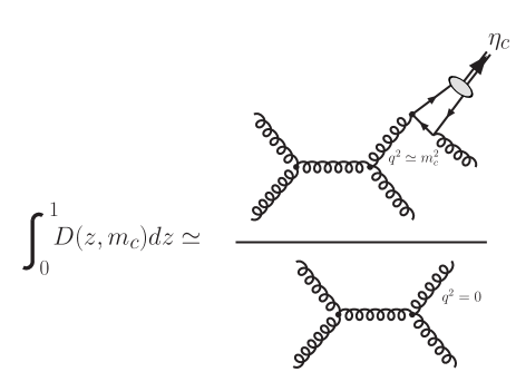
Figure 6: Illustration of how to obtain $\int^{1}_{0}D(z,m_{c})$.

The interesting point raised by Braaten and Yuan is that the fragmentation functions can be calculated perturbatively in $\alpha_{s}$ at the scale $\mu_{frag}=2m_{Q}$. For instance, in the case of gluon fragmentation into an $\eta_{c}$, the trick is to note that $\int^{1}_{0}dzD_{z}(z,m_{c})$ is the ratio to the rates for the well-known $gg\to gg$ process and $gg\to\eta_{c}gg$ (Fig. 6). After some manipulations, the fragmentation function can be obtained from this ratio by identifying the integrand in the $z$ integral. This gives :

$$\begin{split}D_{g\to\eta_{c}}(z,2m_{c})=\frac{1}{6}\alpha^{2}_{s}(2m_{c})\frac{|\psi(0)|^{2}}{m_{c}^{3}}[3z-2z^{2}+2(1-z)\ln(1-z)].\end{split}$$ (7)

The other fragmentation functions of a given parton $i$ into a given quarkonium $\cal Q$, $D_{i\to{\cal Q}}(z,\mu_{frag})$, were obtained in the same spirit. For the Tevatron, the differential cross section versus $p_{T}$ of various CSM fragmentation processes are plotted in Fig. 7 (left).

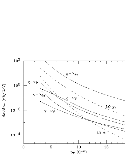
Figure 7: (left) Differential cross section versus $p_{T}$ of various CSM fragmentation processes for $J/\psi$ to be compared with the LO contributions (Reprinted figure from Ref. Braaten:1994xb with permission of Elsevier. Copyright (1994).). (right) Differential cross section versus $p_{T}$ of the CSM (fragmentation and LO) production to be compared with the direct production of $J/\psi$ from CDF (Reprinted figure from Ref. Kramer:2001hh with permission of Elsevier. Copyright (2001).)

The prompt component of the $J/\psi$ and the direct component of the $\psi^{\prime}$ could in turn be obtained and compared with the preliminary data of CDF (see the solid curves in plots in Fig. 5 above). For the $J/\psi$, the previous disagreement was reduced and could be accounted for by the theoretical and experimental uncertainties; on the other hand, for the $\psi^{\prime}$, the disagreement continued to be dramatic. The situation would be clarified by the extraction of the direct component for $J/\psi$, for which theoretical uncertainties are reduced and are similar to those for the $\psi^{\prime}$.

The CDF collaboration undertook the disentanglement of the direct $J/\psi$ signal[49]. They searched for $J/\psi$ associated with the photon emitted during this radiative decay: the result was a direct cross section 30 times above expectations from LO CSM plus fragmentation. This was the confirmation that the CSM was not the suitable model for heavy-quarkonium production in high-energy hadron collisions.

It is a common misconception of the CSM to believe that the well-known factor 30 of discrepancy between data and theory for direct production of $J/\psi$ arises when the data are compared with the predictions for the LO CSM following Baier, Rückl, Chang, …,[27, 28, 29] tuned to the right energy. As you can see on Fig. 7 (right), the factor would be rather of two orders of magnitude at large $p_{T}$ for $J/\psi$. The same conclusion holds also for $\psi^{\prime}$ (see Fig. 5 (right)).

It is also worth pointing that, in the CSM, the direct component of $\psi$ (${}^{3}S_{1}$ charmonia) produced by fragmentation is mainly from $c$-quark fragmentation (see Fig. 7 (left)) as soon as $P_{T}$ reaches 5 GeV and the $\alpha_{s}$ penalty of the gluon fragmentation is not compensated anymore by the $c$-quark mass. It was further pointed out in 2003 by Qiao [51] that sea-quark initiated contributions could dominate in the fragmentation region (large $p_{T}$).

2 Review of contemporary measurements of direct production of $J/\psi$, $\psi^{\prime}$ and $\Upsilon$ from the Tevatron and RHIC

2.1 Foreword

Limiting ourselves to high-energy collisions, the most recent published results for quarkonium hadroproduction come from two accelerators:

1. The Tevatron at Fermilab which – as stated by its name – runs at TeV energy with proton-antiproton collisions. For Run I (“Run IA” 1993-94 and “Run IB” 1995-96), the energy in c.m. was 1.8 TeV. For Run II, it has been increased to 1.96 TeV. The experimental analyses for this Run are still being carried out.

2. RHIC at BNL running at 200 GeV for the $J/\psi$ study with proton-proton collisions.

It is worth pointing out here that high-energy $p$-$\bar{p}$ and $p$-$p$ collisions give similar results for the same kinematics, due to the small contribution of valence quarks.

2.2 Different types of production: prompt, non-prompt and direct

As we have already explained, the detection of quarkonia proceeds via the identification of their leptonic-decay products. We give in Table. 2.2 the relative decay widths into muons.

Table of branching ratios in dimuons (Ref. pdg). Meson $\Gamma(\mu^{+}\mu^{-})/\Gamma(total)$ $J/\psi$ $0.0588\pm 0.0010$ $\psi(2S)$ $0.0073\pm 0.0008$ $\Upsilon(1S)$ $0.0248\pm 0.0006$ $\Upsilon(2S)$ $0.0131\pm 0.0021$ $\Upsilon(3S)$ $0.0181\pm 0.0017$

Briefly, the problem of direct $J/\psi$ production separation comprises three steps:

• muon detection;

• elimination of $J/\psi$ produced by hadrons containing $b$ quarks ;

• elimination of $\chi_{c}$ radiative-decay production;

Table 4 summarises the different processes to be discussed and the quantities linked.

Different processes involved in $J/\psi$ production accompanied by quantities used in the following discussion. $1^{st}$ step $2^{nd}$ step $3^{rd}$ step Type Associated quantity $c\bar{c}\to J/\psi$ $-$ Direct prod. $F(b\!\!\!/,\chi\!\!\!/,\psi\!\!\!/^{\prime})^{J/\psi}$ $p\bar{p}\to c\bar{c}+X$ $c\bar{c}\to\chi_{c}$ $\chi_{c}\to J/\psi+\gamma$ Prompt prod. by decay of$\chi_{c}$ $F(b\!\!\!/)_{\chi}^{J/\psi}$ $c\bar{c}\to\psi^{\prime}$ $\psi^{\prime}\to J/\psi+X$ Prompt prod. by decay of $\psi^{\prime}$ $F(b\!\!\!/)_{\psi^{\prime}}^{J/\psi}$ $\begin{array}[]{c}p\bar{p}\to\bar{b}c+X\\ \bar{b}c\to\bar{c}c+\ell^{-}+\bar{\nu}_{\ell}\end{array}$ $\begin{array}[]{ll}\\ c\bar{c}\to J/\psi\\ c\bar{c}\to\chi_{c}\end{array}$ $\begin{array}[]{cl}\\ -\\ \chi_{c}\to J/\psi+\gamma\end{array}$ $\begin{array}[]{ll}\\ -\\ -\end{array}$ $\begin{array}[]{c}\\ f_{b}(orF_{b})\\ \end{array}$ etc …

Let us explain the different fractions that appear in the table:

• $F(b\!\!\!/,\chi\!\!\!/,\psi\!\!\!/(2S))^{J/\psi}$ is the prompt fraction of $J/\psi$ that do not come $\chi$, neither from $\psi(2S)$, i.e. the direct fraction.

• $F(b\!\!\!/)_{\psi(2S)}^{J/\psi}$ is the prompt fraction of $J/\psi$ that come from $\psi(2S)$.

• $F(b\!\!\!/)_{\chi}^{J/\psi}$ is the prompt fraction of $J/\psi$ that come from $\chi$.

• $F_{b}$ (or $f_{b}$) is the non-prompt fraction or equally the fraction that come for $b$ quarks.

Concerning $\psi(2S)$, due to the absence of stable higher excited states likely to decay into it, we have the summary shown in Table 5 for the different processes to be discussed and the quantities linked:

Different processes involved in $\psi^{\prime}$ production accompanied by quantities used in the following discussion. $1^{st}$ step $2^{nd}$ step $3^{rd}$ step Type Associated quantity $p\bar{p}\to c\bar{c}+X$ $c\bar{c}\to\psi(2S)$ $-$ Direct/Prompt prod. $F(b\!\!\!/)^{\psi(2S)}$ $\begin{array}[]{c}p\bar{p}\to\bar{b}c+X\\ \bar{b}c\to\bar{c}c+\ell^{-}+\bar{\nu}_{\ell}\end{array}$ $c\bar{c}\to\psi(2S)$ $-$ $-$ $f_{b}(orF_{b})$ etc …

Let us explain the different fractions that appear in the corresponding table:

• $F(b\!\!\!/)^{\psi(2S)}$ is the prompt fraction of $\psi(2S)$, i.e. the direct production.

• $F_{b}$ (or $f_{b}$) is the non-prompt fraction or equally the fraction that come for $b$ quarks.

As can be seen in Table. 2.2, the leptonic branching ratio of $\Upsilon$ are also relatively high. The detection and the analysis of the bottomonia are therefore carried out in the same fashion. For the extraction of the direct production, the $b$-quark feed-down is obviously not relevant, only the decays from stable higher resonances of the family are to be considered.

All the quantities useful for the bottomonium discussion are summarised in Table 6:

Different processes involved in $\Upsilon(nS)$ ($n=1,2,3$) production accompanied by quantities used in the following discussion. $1^{st}$ step $2^{nd}$ step $3^{rd}$ step Type Associated quantity $p\bar{p}\to b\bar{b}+X$ $b\bar{b}\to\Upsilon(nS)$ $-$ Direct prod. $F_{direct}^{\Upsilon(nS)}$ $b\bar{b}\to\chi_{b}$ $\chi_{b}\to\Upsilon(nS)+\gamma$ Prod. by decay of $\chi_{b}$ $F_{\chi_{b}}^{\Upsilon(nS)}$ $b\bar{b}\to\Upsilon(n^{\prime}S)$ $\Upsilon(nS)\to\Upsilon(n^{\prime}S)+X$ Prod. by decay of $\Upsilon(n^{\prime}S)$ $F_{\Upsilon(n^{\prime}S)}^{\Upsilon(nS)}$

Let us explain the different fractions that appear in the latter table:

• $F_{direct}^{\Upsilon(nS)}$ is the direct fraction of $\Upsilon(nS)$.

• $F_{\chi_{b}}^{\Upsilon(nS)}$ is the fraction of $\Upsilon(nS)$ that come from $\chi_{b}$.

• $F_{\Upsilon(n^{\prime}S)}^{\Upsilon(nS)}$ is the fraction of $\Upsilon(nS)$ that come from a higher $\Upsilon(n^{\prime}S)$.

2.3 CDF analysis for $\psi$ production cross sections

The sample of $p\bar{p}$ collisions amounts to $17.8\pm 0.6$ pb^-1 at $\sqrt{s}=1.8$ TeV [41]. For $J/\psi$, the considered sample consists however of $15.4\pm 0.6$ pb^-1 of integrated luminosity.

The number of $\psi$ candidates is therefore determined by fitting the mass distribution of the muons in the c.m. frame after subtraction of the noise. The mass distribution is fit to the signal shape fixed by simulation and to a linear background. The fit also yields the mass of the particle and a background estimate.

From the branching ratio and after corrections due to the experimental efficiency, the number of produced particles is easily obtained from the number of the candidates.

For the present study of CDF, the fits are reasonably good for each $p_{T}$-bin, the $\chi^{2}$ per degree of freedom ranging from 0.5 to 1.5. The measured width of the mass peak was from 17 MeV to 35 MeV for $p_{T}$ from 5 to 20 GeV.

Approximatively, 22100 $J/\psi$ candidates and 800 $\psi^{\prime}$ candidates above a background of 1000 events are observed. The $J/\psi$ efficiency is $97.0\pm 0.2\%$ and the $\psi^{\prime}$ one is $92.3\pm 0.2\%$[41].

The integrated cross sections are measured to be

$$\sigma(J/\psi)\cdot{\cal B}(J/\psi\to\mu^{+}\mu^{-})=17.4\pm 0.1(stat.)^{+2.6}_{-2.8}(syst.)\ {\rm nb}$$ (8)

$$\sigma(\psi(2S))\cdot{\cal B}(\psi(2S)\to\mu^{+}\mu^{-})=0.57\pm 0.04(stat.)^{+0.08}_{-0.09}(syst.)\ {\rm nb}.$$ (9)

where $\sigma(\psi)\equiv\sigma(p\bar{p}\to\psi X,p_{T}(\psi)>5\hbox{ GeV},|\eta(\psi)|<0.6)$.

2.3.1 Disentangling prompt charmonia

As already seen, prompt $\psi$’s are the ones which do not come from the decay of $B$ mesons. Their production pattern has the distinctive feature, compared to non-prompt ones, that there exists a measurable distance between the $B$ production vertex and its decay into charmonium.

To proceed, CDF uses the SVX, whose resolution is $40\mu$m, whereas $B$ lifetime is $c\tau_{B}\approx 450\mu$m. Muons are constrained to come from the same point which is called the secondary vertex, as opposed to the primary vertex, that is the collision point of protons. Then the projection of the distance between these two vertices on the $\psi$ momentum, $L_{xy}$, can be evaluated. It is converted into a proper time equivalent quantity using the formula, $c\tau=\frac{L_{xy}}{{p_{T}(\psi)\over m(\psi)}\cdot F_{corr}}$, where $F_{corr}$ is a correction factor, estimated by Monte-Carlo simulations, which links the $\psi$ boost factor $\beta_{T}\gamma$ to that of the $B$ [52].

The prompt component of the signal is parametrised by $c\tau=0$ (a single vertex), the component coming from $B$ decay is represented by an exponential, whose lifetime is $\tau_{b}$ and which is convoluted with the resolution function.

The $c\tau$ distribution is fit in each $p_{T}$-bin with an unbinned log-likelihood function. The noise is allowed to vary within the normalisation uncertainty extracted from the sidebands. The fraction of $\psi$ coming from $b$, $f_{b}(p_{T})$, obtained by CDF is displayed as a function of $p_{T}$ in Fig. 8.

Figure 8: Fraction of $\psi$ from $B$ decay as a function of $p_{T}$ (Reprinted figure from Ref. CDF7997a with permission of American Physical Society. Copyright (1997)).

The $\psi$ production cross section from $B$ decays is thus extracted by multiplying $f^{fit}_{b}(p_{T})$ by the inclusive $\psi$ cross section. Multiplying the latter by $(1-f^{fit}_{b}(p_{T}))$, one obviously gets the prompt-production cross section (cf. Fig. 9).

Figure 9: $\frac{d\sigma}{dp_{T}}{\cal B}$ from the prompt component of $\psi$ (data from Ref. CDF7997a).

We remind the reader than for $\psi(2S)$ the prompt production identifies with the direct one.

2.3.2 Disentangling the direct production of $J/\psi$

The problem here is to subtract the $J/\psi$ coming from $\chi_{c}$ decay, assuming that this is the only source of prompt $J/\psi$ besides the direct production after subtraction of $F(b\!\!\!/)_{\psi(2S)}^{J/\psi}$, the prompt fraction of $J/\psi$ that come from $\psi(2S)$. The latter is evaluated by CDF from the $\psi(2S)$ cross section from the previous section and from Monte-Carlo simulation of the decays $\psi(2S)\to~{}J/\psi X$ where $X=\pi\pi$, $\eta$ and $\pi^{0}$. The delicate point here is the detection of the photon emitted during the radiative decay of the $\chi_{c}$.

The sample they use is 34367 $J/\psi$ from which $32642\pm 185$ is the number of real $J/\psi$ when the estimated background is removed.

The requirements to select the photon were as follow:

• an energy deposition of at least 1 GeV in a cell of the central electromagnetic calorimeter;

• a signal in the fiducial volume of the strip chambers (CES);

• the absence of charged particles pointing to the photon-candidate cell (the no-track cut).

The direction of the photon is determined from the location of the signal in the strip chambers and from the event interaction point. All combinations of the $J/\psi$ with all photon candidates that have passed these tests are made and the invariant-mass difference defined as $\Delta M=M(\mu^{+}\mu^{-}\gamma)-M(\mu^{+}\mu^{-})$ can then be evaluated. As expected, the distribution $\Delta M$ shows of a clear peak from $\chi_{c}$ decays is visible near $\Delta M=400$ MeV. Yet, distinct signals for $\chi_{c,1}$ and $\chi_{c,2}$ are not resolved as the two states are separated by 45.6 MeV and as the mass resolution of the detector is predicted to be respectively 50 and 55 MeV.

Eventually, the $\Delta M$ distribution obtained from the data is fit with a gaussian and with the background fixed by the procedure explained above but with a free normalisation. The parameter of the gaussian then leads to the number of signal events: $1230\pm 72$ $\chi_{c}$.

The analysis of the direct $J/\psi$ signal is done within four $p_{T}$-bins: $4<p_{T}^{J/\psi}<6$, $6<p_{T}^{J/\psi}<8$ , $8<p_{T}^{J/\psi}<10$ and $p_{T}^{J/\psi}>10$ GeV. For $p_{T}^{J/\psi}>4.0$ GeV and $|\eta^{J/\psi}|<0.6$, CDF finds that the fraction of $J/\psi$ from $\chi_{c}$ is then

$$F_{\chi}^{J/\psi}=27.4\%\pm 1.6\%(stat.)\pm 5.2\%(syst.)$$ (10)

The last step now is the disentanglement of the prompt $\chi_{c}$ production, that is the determination of $F(b\!\!\!/)_{\chi}^{J/\psi}$. Let us here draw the reader’s attention to the fact that by selecting prompt $J/\psi$ (cf. section 2.3.1), $J/\psi$ produced by non-prompt $\chi_{c}$ have also been eliminated; it is thus necessary to remove only the prompt production by $\chi_{c}$ decay, and nothing else. This necessitates the knowledge of $F(b\!\!\!/)_{\chi}^{J/\psi}$, the prompt fraction of $J/\psi$ that come from $\chi$.

The latter is calculated as follows:

$$\begin{split}F(b\!\!\!/)_{\chi}^{J/\psi}=F_{\chi}^{J/\psi}\frac{1-F^{\chi}_{b}}{1-F^{J/\psi}_{b}},\end{split}$$ (11)

where $N_{b}^{\chi}$, $N_{b}^{J/\psi}$ are the number of reconstructed $\chi_{c}$ and $J/\psi$ from $b$’s, $F_{b}^{\chi}$, $F_{b}^{J/\psi}$ are the corresponding fractions.

$F_{b}^{J/\psi}$ (or $f_{b}$) is known as seen in the section 2.3.1; $F_{b}^{\chi}$ is obtained in same way and is $17.8\%\pm 0.45\%$ for $p_{T}>4.0$ GeV. Consequently,

$$F(b\!\!\!/)_{\chi}^{J/\psi}=29.7\%\pm 1.7\%(stat.)\pm 5.7\%(syst.)$$ (12)

and its evolution as a function of $p_{T}$ is shown in Fig. 10 (left) . It is also found that the fraction of directly produced $J/\psi$ is

$$F_{direct}^{J/\psi}=64\%\pm 6\%,$$ (13)

and is almost constant from 5 to 18 GeV in $p_{T}$ (see Fig. 10 (left)). We therefore conclude from the analysis of CDF that the direct production is the principal contribution to $J/\psi$.

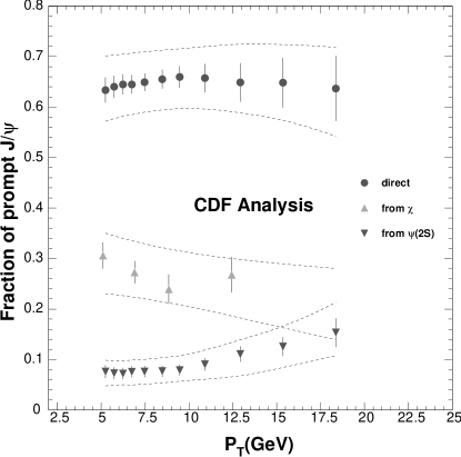
Figure 10: (left) Fractions of $J/\psi$ with the contribution of $b$’s removed. The error bars correspond to statistical uncertainty. The dashed lines show the upper and lower bounds corresponding to the statistical and systematic uncertainties combined (from new1). (right) Differential cross section for prompt production of $J/\psi\to\mu^{-}\mu^{+}$ as a function of $p_{T}$ (Reprinted figure from Ref. CDF7997b with permission of American Physical Society. Copyright (1997)).

In order to get the cross section of direct $J/\psi$ production, it is sufficient now to extract the contribution of $\psi^{\prime}$ obtained by Monte-Carlo simulation and of $\chi_{c}$ obtained by multiplying the cross section of prompt production by the factor $F(b\!\!\!/)_{\chi}^{J/\psi}$, which is a function of $p_{T}^{J/\psi}$. The different cross sections are displayed in Fig. 10 (right).

2.3.3 Prompt $J/\psi$ production at $\sqrt{s}=1.96~{}{\rm TeV}$

The first results of the run II for prompt $J/\psi$ production at $\sqrt{s}=1.96$ TeV have recently been published in Ref. Acosta:2004yw. They correspond to an integrated luminosity of 39.7 pb^-1. The inclusive $J/\psi$ cross section was measured for $P_{T}$ from 0 to 20 GeV and the prompt signal was extracted from $P_{T}=1.25$ GeV. The rapidity domain is still $-0.6<y<0.6$.

We do not give here the details of the experimental analysis which is thoroughly exposed in Ref. Acosta:2004yw. The prompt-signal extraction follows the same lines as done for the analysis previously exposed. The prompt $J/\psi$ cross section obtained is plotted in Fig. 11.

Figure 11: Prompt $J/\psi$ cross section as measured by CDF at $\sqrt{s}=1.96$ TeV (statistical and systematical errors have been combined quadratically for this plot); the data are from Ref. Acosta:2004yw.

2.4 CDF measurement of the $\Upsilon$ production cross sections

In this section, the results by CDF on $\Upsilon$ production in $p\bar{p}$ at $\sqrt{s}=1.8$ TeV are exposed. These results were exposed in two Letters (Refs. CDF7595,Acosta:2001gv), and we shall mainly focus on the second one, which considered data collected in 1993-95 and corresponding to an integrated luminosity of $77\pm 3$ pb^-1. The number of candidates are $4430\pm 95$ for $\Upsilon(1S)$, $1114\pm 65$ for $\Upsilon(2S)$ and $584\pm 53$ for $\Upsilon(3S)$.

The cross section for $\Upsilon(1S)$ is shown in Fig. 12 (left), for $\Upsilon(2S)$ in Fig. 12 (middle) and for $\Upsilon(3S)$ in Fig. 12 (right).

Figure 12: left: Differential cross section of $\Upsilon(1S)\to\mu^{-}\mu^{+}$ as a function of $p_{T}$ for $|y|<0.4$. middle: Idem for $\Upsilon(2S)\to\mu^{-}\mu^{+}$. right: Idem for $\Upsilon(3S)\to\mu^{-}\mu^{+}$ (data from Ref. Acosta:2001gv).

2.4.1 Disentangling the direct production of $\Upsilon(1S)$

The analysis[57] presented here is for the most part the same as described in section 2.3.2. It is based on 90 pb^-1 of data collected during the 1994-1995 run. The measurement has been constrained to the range $p_{T}>8.0$ GeV because the energy of the photon emitted during the decay of $\chi_{b}$ decreases at low $p_{T}$ and ends up to be too small for the photon to be detected properly. In the same spirit, analysis relative to $\Upsilon(2S)$ has not been carried out, once again because of the lower energy of the radiative decay. Concerning $\Upsilon(3S)$, except for the unobserved $\chi_{b}(3P)$ (which is nevertheless supposed to be below the $B\bar{B}$ threshold), no states are supposed to be possible parents.

A sample of 2186 $\Upsilon(1S)$ candidates is obtained from which $1462\pm 55$ is the estimated number of $\Upsilon(1S)$ after subtraction of the background. In the sample considered, photons likely to come from $\chi_{b}$ decay are selected as for the $J/\psi$ case, except for the energy deposition in the central electromagnetic calorimeter, which is lowered to 0.7 GeV.

For $p_{T}^{\Upsilon(1S)}>8.0$ GeV and $|\eta^{\Upsilon(1S)}|<0.7$, the fractions of $\Upsilon(1S)$ from $\chi_{b}(1P)$ and from $\chi_{b}(2P)$ are measured by CDF to be

$$\begin{split}F_{\chi_{b}(1P)}^{\Upsilon(1S)}=&27.1\%\pm 6.9\%(stat.)\pm 4.4\%(syst.),\\ F_{\chi_{b}(2P)}^{\Upsilon(1S)}=&10.5\%\pm 4.4\%(stat.)\pm 1.4\%(syst.).\end{split}$$ (14)

The feed-down from the $S$-waves $\Upsilon(2S)$ and $\Upsilon(3S)$ is obtained by Monte-Carlo simulations of these decays normalised to the production cross sections discussed in section 2.4. It is found that for $p_{T}^{\Upsilon(1S)}>8.0$ GeV the fraction of $\Upsilon(1S)$ from $\Upsilon(2S)$ and $\Upsilon(3S)$ are respectively

$$\begin{split}F_{\Upsilon(2S)}^{\Upsilon(1S)}=10.1\%^{+7.7}_{-4.8}\%,F_{\Upsilon(3S)}^{\Upsilon(1S)}=0.8\%^{+0.6}_{-0.4}\%.\end{split}$$ (15)

Concerning the unobserved $\chi_{b}(3P)$, a maximal additional contribution is taken into account by supposing than all the $\Upsilon(3S)$ are due to $\chi_{b}(3P)$ and from theoretical expectation for the decay of this state, a relative rate of $\Upsilon(1S)$ from $\chi_{b}(3P)$ can obtained. This rate is less than $6\%$.

Eventually the fraction of directly produced $\Upsilon(1S)$ is found to be

$$\begin{split}F_{direct}^{\Upsilon(1S)}&=50.9\%\pm 8.2\%(stat.)\pm 9.0\%(syst.).\end{split}$$ (16)

2.5 Polarisation study

As the considered bound states, $\psi$ and $\Upsilon$ are massive spin-1 particles, they have three polarisations. In addition to measurements of their momentum after their production, the experimental set-up of CDF is sufficiently refined to provide us with a measurement of their spin alignment through an analysis of the angular distribution of the dimuon pairs from the decay.

The CDF collaboration has carried out two analyses, one for the $\psi$ states[59] – for which the feed-down from $b$ decay has been subtracted, but not the indirect component in the case of the $J/\psi$ – and another for $\Upsilon(nS)$ [56].

In the following, we shall proceed to a brief outline of the analysis and give its main results.

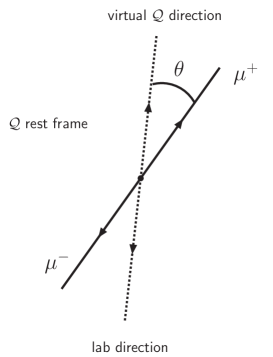
Figure 13: Definition of the angle $\theta$ used in the polarisation analysis of a quarkonium ${\cal Q}$.

The polarisation state of the quarkonium can be deduced from the angular dependence of its decay into $\mu^{+}\mu^{-}$. Taking the spin quantisation axis along the quarkonium momentum direction in the $p\bar{p}$ c.m. frame, we define $\theta$ as the angle between the $\mu^{+}$ direction in the quarkonium rest frame and the quarkonium direction in the lab frame (see Fig. 13). Then the normalised angular distribution $I(\cos\theta)$ is given by

$$\begin{split}I(\cos\theta)=\frac{3}{2(\alpha+3)}(1+\alpha\ \cos^{2}\theta)\end{split}$$ (17)

where the interesting quantity is

$$\begin{split}\alpha=\frac{\frac{1}{2}\sigma_{T}-\sigma_{L}}{\frac{1}{2}\sigma_{T}+\sigma_{L}}.\end{split}$$ (18)

$\alpha=0$ means that the mesons are unpolarised, $\alpha=+1$ corresponds to a full transverse polarisation and $\alpha=-1$ to a longitudinal one.

As the expected behaviour is biased by muons cuts – for instance there exists a severe reduction of the acceptance as $\theta$ approaches 0 and 180 degrees, due to the $p_{T}$ cuts on the muons –, the method followed by CDF was to compare measurements, not with a possible $(1+\alpha\ \cos^{2}\theta)$ distribution, but with distributions obtained after simulations of quarkonium decays taking account the geometric and kinematic acceptance of the detector as well as the reconstruction efficiency.

The parts of the detector used are the same as before, with the additional central muon upgrade (CMP) outside the CMU.

2.5.1 Study of the $\psi$’s polarisation by CDF

We give here the results relative to the CDF analysis published in 2000 [59]. The data used correspond to an integrated luminosity of 110 pb^-1 collected between 1992 and 1995.

Disentangling prompt production for $\psi$

The measured fraction of $J/\psi$ mesons which come from $b$-hadron decay, $F^{J/\psi}_{b}$, is measured to increase from $(13.0\pm 0.3)\%$ at $p_{T}=4$ GeV to $(40\pm 2)\%$ at 20 GeV and for $\psi^{\prime}$ mesons, $F^{\psi^{\prime}}_{b}$ is $(21\pm 2)\%$ at 5.5 GeV and $(35\pm 4)\%$ at 20 GeV.

Within a 3-standard-deviation mass window around the $J/\psi$ peak, the data sample is of 180 000 $J/\psi$ events. In order to study the effect of $p_{T}$, the data are divided into seven $p_{T}$-bins from 4 to 20 GeV. Because the number of $\psi^{\prime}$ events is lower, data for $\psi^{\prime}$ are divided into three $p_{T}$-bins from 5.5 to 20 GeV.

$J/\psi$ polarisation measurement

The polarisation is obtained using a $\chi^{2}$ fit of the data to a weighted sum of transversely polarised and longitudinally polarised templates. The weight obtained with the fit provides us with the polarisation. Explanations relative to procedure used can be found in Refs. Affolder:2000nn and Cropp:2000zk.

Note however that the polarisation is measured in each $p_{T}$ bin and that separate polarisation measurements for direct $J/\psi$ production and for production via $\chi_{c}$ and $\psi^{\prime}$ decays was found to be unfeasible. Let us recall here that $\chi_{c}$ and $\psi^{\prime}$ were shown to account for 36$\pm$6% of the prompt production (cf. Eq. (13)) and to be mostly constant in the considered $p_{T}$ range.

Except in the lowest $p_{T}$ bins, the systematic uncertainties are much smaller than the statistical one. The values obtained for $\alpha_{Prompt}$ and $\alpha_{fromB}$ are given in Table. 2.5.1 and plotted in Fig. 14.

Fit results for $J/\psi$ polarisation, with statistical and systematic uncertainties (Ref. Affolder:2000nn). $p_{T}$ bin (GeV) Mean $P_{T}$ (GeV) $\alpha_{Prompt}$ $\alpha_{fromB}$ $4-5$ 4.5 $0.30\pm 0.12\pm 0.12$ $-0.49\pm 0.41\pm 0.13$ $5-6$ 5.5 $0.01\pm 0.10\pm 0.07$ $-0.18\pm 0.33\pm 0.07$ $6-8$ 6.9 $0.178\pm 0.072\pm 0.036$ $0.10\pm 0.20\pm 0.04$ $8-10$ 8.8 $0.323\pm 0.094\pm 0.019$ $-0.06\pm 0.20\pm 0.02$ $10-12$ 10.8 $0.26\pm 0.14\pm 0.02$ $-0.19\pm 0.23\pm 0.02$ $12-15$ 13.2 $0.11\pm 0.17\pm 0.01$ $0.11\pm^{0.31}_{0.28}\pm 0.02$ $15-20$ 16.7 $-0.29\pm 0.23\pm 0.03$ $-0.16\pm^{0.38}_{0.33}\pm 0.05$

Figure 14: $\alpha_{Prompt}$ for $J/\psi$ fit for $|y|<0.6$. The error bars denote statistical and systematic uncertainties added in quadrature.

$\psi^{\prime}$ polarisation measurement

The procedure to obtain $\alpha_{Prompt}$ and $\alpha_{fromB}$ is similar. Weighted simulations of the angular distribution are fit to the data and the weight obtained gives the polarisation. The $|\cos\theta|$ distributions in the two $c\tau$ sub-samples are fit simultaneously. As there is no expected radiative decay from higher excited charmonia, we are in fact dealing with direct production.

Anew, the systematic uncertainties[59] are much smaller than the statistical uncertainties. The values obtained for $\alpha_{Prompt}$ and $\alpha_{fromB}$ are given in Table. 2.5.1 and plotted in Fig. 15.

Figure 15: $\alpha_{Prompt}$ for $\psi^{\prime}$ fit for $|y|<0.6$. Error bars denote statistical and systematic uncertainties added in quadrature.

Fit results for $\psi(2S)$ polarisation, with statistical and systematic uncertainties (Ref. Affolder:2000nn). $p_{T}$ bin (GeV) Mean $p_{T}$ (GeV) $\alpha_{Prompt}$ $\alpha_{fromB}$ $5.5-7.0$ 6.2 $-0.08\pm 0.63\pm 0.02$ $-0.26\pm 1.26\pm 0.04$ $7.0-9.0$ 7.9 $0.50\pm 0.76\pm 0.04$ $-1.68\pm 0.55\pm 0.12$ $9.0-20.0$ 11.6 $-0.54\pm 0.48\pm 0.04$ $0.27\pm 0.81\pm 0.06$

2.5.2 Study of the $\Upsilon(1S)$

The measurements are made in the region of $p_{T}$ from 0 to 20 GeV and with $|y|<0.4$ and the data are separated in four $p_{T}$-bins[56]. In Table. 2.5.2 are given the results for $\alpha$ and the same values are plotted in Fig. 16. Our conclusion is that $\Upsilon(1S)$ seems to be mostly produced unpolarised.

Figure 16: $\alpha$ for $\Upsilon(1S)$ fit for $|y|<0.4$.

Fit results for $\Upsilon(1S)$ polarisation (Ref. Acosta:2001gv). $p_{T}$ bin (GeV) $\alpha$ $0.0-3.0$ $+0.05\pm 0.14$ $3.0-5.0$ $+0.01\pm 0.14$ $5.0-8.0$ $+0.10\pm 0.17$ $8.0-20.0$ $-0.12\pm 0.22$

2.5.3 New preliminary measurements by CDF for prompt $J/\psi$

To complete the review of the measurements of quarkonium polarisation done by the CDF collaboration, we give in Fig. 17 the preliminary one for prompt $J/\psi$ for RUN II with an integrated luminosity of $188\pm 11$ pb^-1 for $J/\psi$ with $5\leq P_{T}\leq 30$ GeV and $|y|\leq 0.6$.

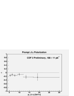
Figure 17: Preliminary measurements of the prompt production of $J/\psi$ as measured by CDF for RUN II (from Ref. pol_prelim).

2.6 PHENIX analysis for $J/\psi$ production cross sections

In this section, we present the first measurements of $pp\to J/\psi+X$ at RHIC obtained by the PHENIX experiment[61] at a c.m. energy of $\sqrt{s}=200$ GeV. The analysis was carried out by detecting either dielectron or dimuon pairs. The data were taken during the run at the end of 2001 and at the beginning of 2002. The data amounted to 67 nb^-1 for $\mu^{+}\mu^{-}$ and 82 nb^-1 for $e^{+}e^{-}$. The $B$-decay feed-down is estimated to contribute less than 4% at $\sqrt{s}=200$ GeV and is not studied separately. The production is thus assumed here to be nearly totally prompt, feed-down from $\chi_{c}$ is expected to exist though[62, 63].

The net yield of $J/\psi$ within the region $2.80\hbox{ GeV}<M(pair)<3.40\hbox{ GeV}$ was found to be $46.0\pm 7.4$ for electrons, whereas for muons, it was $65.0\pm 9.5$ $J/\psi$ within the region $2.71\hbox{ GeV}<M(pair)<3.67\hbox{ GeV}$. The cross section as a function of $p_{T}$ is shown for the two analyses on Fig. 18.

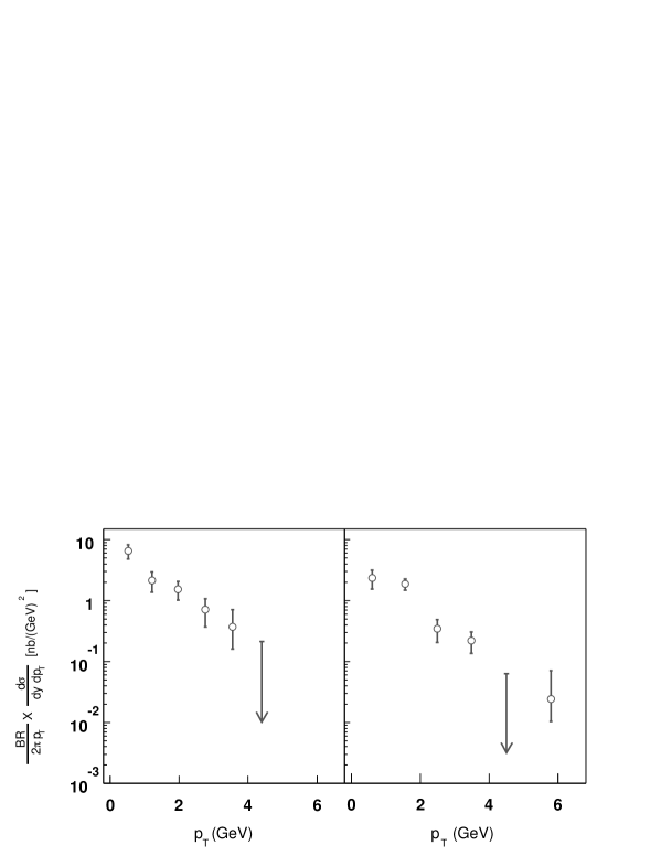
Figure 18: The differential cross section measured: left for dielectrons, right for dimuons (Ref. Adler:2003qs).

3 Review of contemporary models for production at the Tevatron and RHIC

3.1 Soft-Colour Interaction vs Colour Evaporation Model

Introduced[64, 65] as a new way to explain the observation of rapidity gaps in deep inelastic scattering at HERA, the Soft-Colour Interaction (SCI) model was also applied to quarkonium production, in particular in the context of hadron-hadron collisions (Tevatron[66] and LHC[67]).

The main idea of the model is to take into consideration soft interactions occurring below a small momentum scale, which we shall call here $Q_{0}^{2}$, in addition to those considered in the hard interaction through Feynman graphs. Unfortunately, we do not have satisfactory tools to deal with such soft QCD interactions. Nevertheless, the interesting point of these interaction –emphasised by the SCI model– lies in the fact that these matter only for colour, since they cannot affect significantly the parton momenta. Therefore, one possibility is to implement them via Monte Carlo (MC) event generators by solely exchanging the colour state of two selected softly interacting partons with a probability $R$. From rapidity gap studies, $R$ is close to 0.5.

3.1.1 The model in hadroproduction

To what concerns the hard part, Edin et al. followed a procedure similar to the CEM: the prompt cross section to get a given quarkonium $\cal Q$ is obtained from the one to get a colour-singlet $Q\bar{Q}$ pair with an invariant mass between $2m_{Q}$ and $2m_{\bar{q}Q}$ after distributing it between the different states of a family (charmonium or bottomonium). In the CEM, it is supposed –from $SU(3)$ counting– to be one ninth of the total cross section $\sigma_{Q\bar{Q}}$.

The latter can be computed by Monte Carlo (MC) event generators, which can be coupled to the SCI procedure (possible exchange of colour state between some partons). The computation of $\sigma_{Q\bar{Q}}$ can be effectively done either with NLO matrix elements (which include gluon-fragmentation into a colour-octet pair) or with Pythia[69] –including LO matrix elements and parton showers– (which also contains gluon-fragmentation into a colour-octet pair). Choosing Pythia has the advantage of introducing even higher contributions which can be significant. To illustrate this, we have reproduced a comparison (see Fig. 19) of two CEM calculations: one with NLO matrix-element implementation and another with Pythia Monte Carlo including parton showers. $m_{c}$ was set to 1.5 GeV, $\rho_{J/\psi}$ was taken to be 0.5, and $\rho_{\psi^{\prime}}$ 0.066. These two choices disagree clearly with simple spin statistics, but are necessary to reproduce the normalisation of the data.

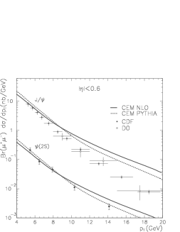
Figure 19: Comparison between $J/\psi$ and $\psi^{\prime}$ prompt production cross sections within CEM with NLO matrix elements and with Pythia. The data are from CDF [55] and D$\emptyset$ [70] (Reprinted figure from Ref. Mariotto:2001sv with kind permission of Springer Science and Business Media. Copyright (2002)).

3.1.2 The results of the model

The cross section to produce the colour-singlet heavy-quark pair (see Eq. (4)) is computed here with Pythia which is coupled to the SCI model: once the selected partons –with a probability $R$– have exchanged their colour, only the events producing a colour-singlet heavy-quark pair are retained. This directly gives the singlet-state cross section, whereas in the CEM $\frac{1}{9}\sigma_{Q\bar{Q}}$ is used. It is also integrated in the mass region between $2m_{Q}$ and $2m_{\bar{q}Q}$. The cross section to produce one given quarkonium $\cal Q$ is obtained using:

$$\begin{split}\sigma_{\cal Q}=\frac{\Gamma_{\cal Q}}{\sum_{i}\Gamma_{i}}\sigma_{onium},\end{split}$$ (19)

with $\Gamma_{i}=\frac{2J_{i}+1}{n_{i}}$ where $J_{i}$ is the total angular momentum and $n_{i}$ the main quantum number. $\rho_{\cal Q}$ is thus effectively replaced by $\frac{\Gamma_{\cal Q}}{\sum_{i}\Gamma_{i}}$ and is not free to vary anymore.

The effect of SCI can be either to turn a colour-singlet pair into a colour-octet one or the contrary. The latter case is important, since it opens the possibility of gluon fragmentation into a quarkonium at order $\alpha^{3}_{s}$ (see Fig. 20). This explains why the model reaches a reasonable agreement with data to what concerns the slope vs $p_{T}$ – the same is equally true for the CEM. Note that the effect of SCI’s on the cross section depends on the partonic state (through the number of possible SCI’s), and thus on the transverse momentum of the produced quarkonium. The final colour-singlet $p_{T}$ slope is slightly steeper than the initial $Q\bar{Q}$ one and in better agreement with data (compare Fig. 19 and Fig. 21 (left))

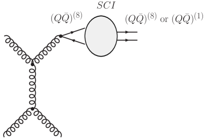
Figure 20: Gluon fragmentation process (part of NLO contributions) giving a singlet state through SCI.

The very interesting point of this approach is its simplicity. $R$ is the only free parameter and is kept at 0.5, which is the value chosen to reproduce the rate of rapidity gaps. However, the cross section depends little on it. Putting $R$ to 0.1 instead of 0.5 decreases the cross section by 30%.

On the other hand, in Eq. (19), the $\frac{1}{n}$ suppression for radially excited states does not fundamentally follow from spin statistics; it is solely motivated by the ratio of the leptonic decay width.

Another drawback is the strong dependence upon the heavy-quark mass. This is mainly due to modified boundary values in the integral from $2m_{Q}$ to $2m_{\bar{q}Q}$, much less to a change in the hard scale and in the mass value entering the matrix elements. Changing $m_{c}$ from 1.35 GeV to 1.6 GeV decreases the cross section by a factor of 3, and from 1.35 GeV to 1.15 GeV increases it by a factor of 2. The other dependences (on $\Lambda_{QCD}$, PDF sets, …) are not significant.

  

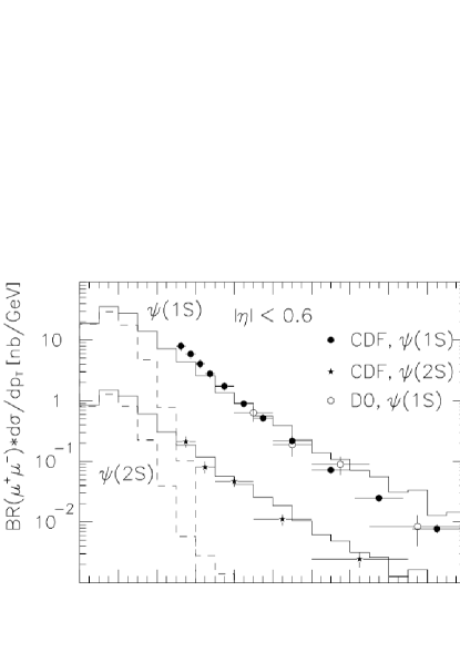
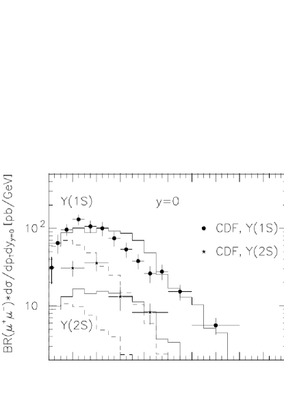
Figure 21: SCI calculations for prompt production of $J/\psi$, $\psi^{\prime}$ (left) and $\Upsilon(1S)$ and $\Upsilon(2S)$ (right). The dashed lines correspond to the LO matrix-element alone, the solid one to the LO matrix-elements with parton showers (Reprinted figures from Ref. Edin:1997zb with permission of American Physical Society. Copyright (1997)).

3.1.3 Improving the mapping

As one can imagine, physically, during the transition between the $Q\bar{Q}$ pair –produced by the hard interaction with an invariant mass between $2m_{Q}$ and $2m_{\bar{q}Q}$– and the physical quarkonium $\cal Q$, this invariant mass is likely to be modified. It is then reasonable to suppose[68] that it is smeared to a mass $m$ around its initial value $m_{Q\bar{Q}}$ with such distribution:

$$\begin{split}G_{sme}(m_{Q\bar{Q}},m)=\exp\left(-\frac{(m_{Q\bar{Q}}-m)}{2\sigma_{sme}}\right).\end{split}$$ (20)

Supposing that the width of the quarkonium resonances tends to zero, the probability that a pair with an invariant mass $m_{Q\bar{Q}}$ gives a quarkonium ${\cal Q}_{i}$ is given by:

$$\begin{split}{\cal P}_{i}(m_{Q\bar{Q}})\simeq\frac{\Gamma_{i}G_{sme}(m_{Q\bar{Q}},m_{{\cal Q}_{i}})}{\sum_{j}\Gamma_{j}G_{sme}(m_{Q\bar{Q}},m_{{\cal Q}_{j}})},\end{split}$$ (21)

still with $\Gamma_{i}=\frac{2J_{i}+1}{n_{i}}$.

This smearing enables quark pairs with invariant masses above the heavy-meson threshold $2m_{\bar{q}Q}$ to produce stable quarkonia, but the reverse is true also, with a probability $A(m_{Q\bar{Q}})$ equal to $\frac{1}{2}\hbox{erfc}\left(\frac{2m_{\bar{q}Q}-m_{Q\bar{Q}}}{\sqrt{2\pi}\sigma_{sme}}\right)$.

The cross section to get a quarkonium ${\cal Q}_{i}$ is thus given Ref. Mariotto:2001sv by

$$\begin{split}\sigma_{i}=\int^{\sqrt{s}}_{2m_{Q}}dm_{Q\bar{Q}}\frac{d\sigma_{Q\bar{Q}}}{dm_{Q\bar{Q}}}(1-A(m_{Q\bar{Q}})){\cal P}_{i}(m_{Q\bar{Q}}),\end{split}$$ (22)

with $\frac{d\sigma_{Q\bar{Q}}}{dm_{Q\bar{Q}}}$ calculated either within CEM (with $\frac{1}{9}$ from $SU(3)$) or within SCI.

Using this procedure, the production ratio $\psi^{\prime}$ over $J/\psi$ is better reproduced[68] than for simple spin statistics as well as the different components of the prompt $J/\psi$ as measured by CDF[49]. On the other hand, due to the proximity in mass of the $\chi_{c1}$ and $\chi_{c2}$, their production ratio is not affected and remains $3:5$ slightly in contradiction with the CDF measurements[71] consistent with a ratio of 1. Finally, this refinement affects the cross sections only by a factor of 20%, what is well within the model uncertainty.

3.2 NRQCD: including the colour-octet mechanism

In 1992, Bodwin et al. considered new Fock-state contributions in order to cancel exactly the IR divergence in the light-hadron decays of $\chi_{c1}$ (and $h_{c}$) at LO. This decay proceeds via two gluons, one real and one off-shell, which gives the light-quark pair forming the hadron. When the first gluon becomes soft, the decay width diverges. The conventional treatment[72, 73, 74, 75], which amounts to regulating the divergence by an infrared cut-off identified with the binding energy of the bound state, was not satisfactory: it supposed a logarithmic dependence of $\Psi^{\prime}(0)$ upon the binding energy. They looked at this divergence as being a clear sign that the factorisation was violated in the CSM.

Their new Fock states for $\chi_{c}$ were e.g. a gluon plus a $c\bar{c}$ pair, in a ${}^{3}S_{1}$ configuration and in a colour-octet state. The decay of this Fock state occurred through the transition of the coloured pair into a gluon (plus the other gluon already present in the Fock state as a spectator). This involved a new phenomenological parameter, $H_{8}$, which was related to the probability that the $c\bar{c}$ pair of the $\chi_{c}$ be in a colour-octet $S$-wave state. The key point of this procedure was that a logarithmic dependence on a new scale $\Lambda$ – a typical momentum scale for the light quark – appeared naturally within the effective field theory Non-Relativistic Quantum Chromodynamic (NRQCD)[76, 77].

This effective theory is based on a systematic expansion in both $\alpha_{s}$ and $v$, which is the quark velocity within the bound state. For charmonium, $v_{c}^{2}\simeq 0.23$ and for bottomonium $v_{b}^{2}\simeq 0.08$. One of the main novel features of this theory is the introduction of dynamical gluons in the Fock-state decomposition of the physical quarkonium states. In the case of $S$-wave orthoquarkonia (${}^{3}S_{1}$), we schematically have, in the Coulomb gauge:

$$\begin{split}|{\cal Q}_{Q}\rangle=&{\cal O}(1)|Q\bar{Q}[\ ^{3}S_{1}^{(1)}]\rangle+{\cal O}(v)|Q\bar{Q}[\ ^{3}P_{J}^{(8)}g]\rangle+{\cal O}(v^{2})|Q\bar{Q}[\ ^{1}S_{0}^{(8)}g]\rangle\\ &+{\cal O}(v^{2})|Q\bar{Q}[\ ^{3}S_{1}^{(1,8)}gg]\rangle+{\cal O}(v^{2})|Q\bar{Q}[\ ^{3}D_{J}^{(1,8)}gg]\rangle+\dots\end{split}$$ (23)

whereas for $P$-wave orthoquarkonia (${}^{3}P_{J}$), the decomposition is as follows

$$\begin{split}|{\cal Q}_{Q_{J}}\rangle=&{\cal O}(1)|Q\bar{Q}[\ ^{3}P_{J}^{(1)}]\rangle+{\cal O}(v)|Q\bar{Q}[\ ^{3}S_{1}^{(8)}g]\rangle+\dots\end{split}$$ (24)

In these two formulae, the superscripts (1) and (8) indicate the colour state of the $Q\bar{Q}$ pair. The ${\cal O}(v^{n})$ factors indicate the order in the velocity expansion at which the corresponding Fock state participates to the creation or the annihilation of quarkonia. This follows from the velocity scaling rules of NRQCD (see e.g. Ref. Bodwin:1994jh).

In this formalism, it is thus possible to demonstrate, in the limit of large quark mass, the factorisation between the short-distance – and perturbative – contributions and the hadronisation of the $Q\bar{Q}$, described by non-perturbative matrix elements defined within NRQCD. For instance, the differential cross section for the production of a quarkonium $\cal Q$ associated with some other hadrons $X$ reads

$$\begin{split}d\sigma({\cal Q}+X)=\sum d\hat{\sigma}(Q\bar{Q}[^{2S+1}L_{J}^{(1,8)}]+X)\langle{\cal O}^{\cal Q}[^{2S+1}L_{J}^{(1,8)}]\rangle,\end{split}$$ (25)

where the sum stands for $S$, $L$, $J$ and the colour.

The long-distance matrix element (LDME) $\langle{\cal O}^{\cal Q}[^{2S+1}L_{J}^{(1,8)}]\rangle$ takes account of the transition between the $Q\bar{Q}$ pair and the final physical state ${\cal Q}$. Its power scaling rule comes both from the suppression in $v$ of the Fock-state component $[^{2S+1}L_{J}^{(1,8)}]$ in the wave function of $\cal Q$ and from the scaling of the NRQCD interaction responsible for the transition.

Usually, one defines ${\cal O}^{\cal Q}[^{2S+1}L_{J}^{(1,8)}]$ as the production operator that creates and annihilates a point-like $Q\bar{Q}$ pair in the specified state. This has the following general expression

$$\begin{split}{\cal O}^{\cal Q}[^{2S+1}L_{J}^{(1,8)}]&=\chi^{\dagger}K\psi\left(\sum_{X}\sum_{J_{z}}|{\cal Q}+X\rangle\langle{\cal Q}+X|\right)\psi^{\dagger}K\chi\\ &=\chi^{\dagger}K\psi(a^{\dagger}_{\cal Q}a_{\cal Q})\psi^{\dagger}K\chi,\end{split}$$ (26)

where $\psi$ and $\chi$ are Pauli spinors and the matrix $K$ is a product of colour, spin and covariant derivative factors. These factors can be obtained from the NRQCD lagrangian[77]. For instance, ${\cal O}^{\cal Q}[\ ^{3}S_{1}^{(1)}]=\chi^{\dagger}\vec{\sigma}\psi(a^{\dagger}_{\cal Q}a_{\cal Q})\psi^{\dagger}\vec{\sigma}\chi$. However some transitions require the presence of chromomagnetic ($\Delta L=0$ and $\Delta S=\pm 1$) and chromoelectric ($\Delta L=\pm 1$ and $\Delta S=0$) terms for which the expressions of $K$ are more complicated.

On the other hand, the general scaling rules relative to the LDME’s[50] give:

$$\begin{split}\langle{\cal O}^{\cal Q}[^{2S+1}L_{J}^{(1,8)}]\rangle=v^{3+2L+2E+4M},\end{split}$$ (27)

where $E$ and $M$ are the minimum number of chromoelectric and chromomagnetic transitions for the $Q\bar{Q}$ to go from the state $[^{2S+1}L_{J}^{(1,8)}]$ to the dominant quarkonium ${\cal Q}$ Fock state.

The idea of combining fragmentation as the main source of production with allowed transitions between a $\chi_{c}$ to a ${}^{3}S_{1}$ in a colour-octet state, was applied by Braaten and Yuan[45]. Indeed, similar formulae to the one written for fragmentation within the CSM can be written for fragmentation functions in NRQCD[78]:

$$\begin{split}D_{g\to{\cal Q}}(z,\mu)=\sum d_{[^{2S+1}L_{J}^{(1,8)}]}(z,\mu)\langle{\cal O}^{\cal Q}[^{2S+1}L_{J}^{(1,8)}]\rangle,\end{split}$$ (28)

where $d_{[\cdot]}(z,\mu)$ accounts for short-distance contributions and does not depend on which $\cal Q$ is involved. But since the theoretical predictions for prompt $J/\psi$ production did not disagree dramatically with data and since there was no possible $\chi_{c}$ decay to $\psi^{\prime}$, a possible enhancement of the $\chi_{c}$ cross section by colour-octet mechanism (COM) was not seen at that time as a key-point both for $J/\psi$ and $\psi^{\prime}$ production.

However, in the case of $J/\psi$ and $\psi^{\prime}$ production, COM could still matter, but in a different manner: fragmentation of a gluon into a ${}^{3}P_{J}^{(8)}$ is possible with solely one gluon emission and fragmentation into a ${}^{3}S_{1}^{(8)}$ requires no further gluon emission (at least in the hard process –described by $d_{[\cdot]}(z,\mu)$– and not in the soft process associated with $\cal O$). Concerning the latter process, as two chromoelectric transitions are required for the transition $|c\bar{c}gg\rangle$ to $|c\bar{c}\rangle$, the associated LDME $\langle{\cal O}^{\psi}[^{3}S_{1}^{(8)}]\rangle$ was expected to scale as $m_{c}^{3}v^{7}$. In fact, $d_{[^{3}S_{1}^{(8)}]}$, the contribution to the fragmentation function of the short-distance process $g\to\!\!\ ^{3}S_{1}^{(8)}$ was already known since the paper of Braaten and Yuan[45] and could be used here, as the hard part $d_{[\cdot]}(z,\mu)$ of the fragmentation process is independent of the quarkonium.

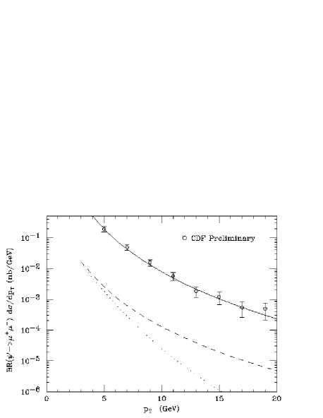
Figure 22: Differential cross section versus $p_{T}$ of the CSM (dotted: LO; dashed: fragmentation and LO) production and of the COM fragmentation (solid curve) to be compared with CDF preliminary measurements of the direct production of $\psi^{\prime}$ [40] (Reprinted figure from Ref. Braaten:1994vv with permission of American Physical Society. Copyright (1995)).

In a key paper, Braaten and Fleming[78] combined everything together to calculate, for the Tevatron, the fragmentation rate of a gluon into an octet ${}^{3}S_{1}$ that subsequently evolves into a $\psi^{\prime}$. They obtained, with $\langle{\cal O}^{\psi(2S)}[^{3}S_{1}^{(8)}]\rangle=4.2\times 10^{-3}$ GeV³, a perfect agreement with the CDF preliminary data[40]: compare these predictions in Fig. 22 with the CSM fragmentation ones in Fig. 5 (right).

Following these studies, a complete survey on the colour-octet mechanism was made in two papers by Cho and Leibovich[79, 80]. The main achievements of these papers were the calculation of colour-octet $P$-state contributions to $\psi$, the predictions for prompt and direct colour-octet $J/\psi$ production with also the $\chi_{c}$ feed-down calculation, the first predictions for $\Upsilon$ and the complete set of $2\to 3$ parton processes like $ij\to c\bar{c}+k$, all this in agreement with the data.

3.2.1 Determination of the LDME’s

Here we expose the results relative to the determination of the Long Distance Matrix Elements of NRQCD necessary to describe the production of ${}^{3}S_{1}$ quarkonium. We can distinct between two classes of matrix elements : the colour singlet ones, which are fixed as we shall see, and the colour octet ones which are fit to reproduce the observed cross sections as a function of $p_{T}$.

In fact, as already mentioned, NRQCD predicts that there is an infinite number of Fock-state contributions to the production of a quarkonium ${\cal Q}$ and thus an infinite number of LDME. Practically, one is driven to truncate the series; this is quite natural in fact since most of the contributions should be suppressed by factor of at least ${\cal O}(\frac{v^{2}}{c^{2}})$, where $v$ is the quark velocity in the bound state.

For definiteness, the latest studies accommodating the production rate of ${}^{3}S_{1}$ states retain only the colour singlet state with the same quantum numbers as the bound state and colour octet $P$-wave states and singlet $S$-wave. In this context, the CSM can be thought as a further approximation to the NRQCD formalism, where we keep solely the leading terms in $v$.

Colour-singlet LDME

In this formalism, factorisation tells us that each contribution is the product of a perturbative part and a non-perturbative matrix element, giving, roughly speaking, the probability that the quark pair perturbatively produced will evolve into the considered physical bound state. If one transposes this to the CSM, this means the wave function at the origin corresponds to this non-perturbative element. This seems reasonable since the wave function squared is also a probability.

Yet, one has to be cautious if one links production processes with decay processes. In NRQCD, two different matrix elements are defined for the “colour singlet” production and decay, and they are likely to be different and independent.

The only path left to recover the CSM is the use of a further approximation, the vacuum saturation approximation. The latter tells us how the matrix element for the decay is linked to the one for the production. This enables us to relate the wave function at the origin appearing in $\Gamma_{\ell\ell}$ (Eq. (3.1) of Ref. Lansberg:2005aw) to the colour-singlet NRQCD matrix element for production. This gives:

$$\begin{split}\langle{\cal O}^{{}^{3}S_{1}}[^{3}S^{(1)}_{1}]\rangle=18\left|\psi(0)\right|^{2}+{\cal O}(v^{4}).\end{split}$$ (29)

The conclusion that could be drawn within NRQCD is that the extraction of non-perturbative input for production from the one for decay is polluted by factors of ${\cal O}(v^{4})$, this is also true for extraction from potential models.

In Table. 3.2.1, we give the colour-singlet LDME for the $J/\psi$ and the $\psi^{\prime}$. The result for the different potentials are deduced from the solutions of Ref. Kopeliovich:2003cn. These LDME’s –up to a factor 18– are those that are to be used in CSM calculations. The values differ from the one used in Refs. CSM_hadron1,CSM_hadron2,CSM_hadron3 because of modifications in the measured values of $\Gamma_{\ell\ell}$, NLO QCD corrections to $\Gamma_{\ell\ell}$ and also in the potential used to obtain the wave function at the origin.

Colour-singlet LDME for the $J/\psi$ and the $\psi^{\prime}$ determined from the leptonic decay width and from various potentials. The error of ${\cal O}(v^{4})$ as shown in Eq. (29) should be implied. Values are given in units GeV³. $\begin{array}[]{|c|c|c|c|c|}\hline\cr\cal Q&\mbox{Leptonic decay}&\mbox{BT Potential Ref.~{}\refcite{Buchmuller:1980bm,Buchmuller:1980su}}&\mbox{POW potential Ref.~{}\refcite{Martin:1980jx}}&\mbox{Cornell Potential Ref.~{}\refcite{cornell_potential1,cornell_potential2}}\\ \hline\cr\hline\cr J/\psi&1.1\pm 0.1&1.16&1.4&2.06\\ \psi^{\prime}&0.7\pm 0.1&0.76&0.76&1.29\\ \hline\cr\end{array}$

In Table. 3.2.1, we expose the results of Ref. Braaten:2000cm concerning the colour-singlet LDME for $\Upsilon(nS)$, i.e. $\langle{\cal{O}}^{\Upsilon(nS)}[{}^{3}S^{(1)}_{1}]\rangle$. The error quoted for the value from potential models expresses the variation of the latter when passing from one to another.

Colour-singlet LDME for the $\Upsilon(nS)$ determined from the leptonic decay width and from potentials models. Values are given in units GeV³ (Ref. Braaten:2000cm). $\footnotesize\begin{array}[]{|c|c|c|}\hline\cr\cal Q&\mbox{Leptonic decay}&\mbox{Potential Models}\\ \hline\cr\hline\cr\Upsilon(1S)&10.9\pm 1.6&10.8\pm 5.5\\ \Upsilon(2S)&4.5\pm 0.7&5.0\pm 1.8\\ \Upsilon(3S)&4.3\pm 0.9&3.7\pm 1.5\\ \hline\cr\end{array}$

Colour-octet LDME’s

As said above, three intermediate colour-octet states are currently considered in the description of ${}^{3}S_{1}$ production. These are ${}^{1}\!S^{(8)}_{0}$, ${}^{3}\!P^{(8)}_{0}$ and ${}^{3}S^{(8)}_{1}$. The corresponding LDME’s giving the probability of transition between these states and the physical colour-singlet ${}^{3}S_{1}$ state are not known and are to be fit to the data.

Unfortunately, the perturbative amplitudes to produce a ${}^{1}\!S^{(8)}_{0}$ or ${}^{3}\!P^{(8)}_{0}$ have the same $p_{T}$ slope and their coefficient cannot be determined apart. Therefore, one defines $k$ as the ratio between these two amplitudes. From it, one defines the following combination

$$\begin{split}M_{k}^{\cal Q}({}^{1}S^{(8)}_{0},{}^{3}P^{(8)}_{0})\equiv\langle{\cal{O}}^{\cal Q}[{}^{1}\!S^{(8)}_{0}]\rangle+k\frac{\langle{\cal{O}}^{\cal Q}[{}^{3}\!P^{(8)}_{0}]\rangle}{m_{c}^{2}},\end{split}$$ (30)

which is fit to the data. In the following, we expose the results obtained by different analyses using various PDF set and parameter values. In the following tables, the first error quoted is statistical, the second error, when present, reflects the variation of the fit LDME when the renormalisation and factorisation scales is set to $\mu=1/2\,\sqrt{p_{T}^{2}+4m_{c}^{2}}$ and to $2\,\sqrt{p_{T}^{2}+4m_{c}^{2}}$. The agreement with the data being actually good, there is no real interest to plot the cross sections given by the fits.

Fit values of $J/\psi$ production LDME’s from $\frac{d\sigma}{dp_{T}}$ at the Tevatron. Values are given in units $10^{-2}$ GeV³ (Numbers from Ref. Kramer:2001hh). $\footnotesize\begin{array}[]{|c||c|c||c|c|c|}\hline\cr\mbox{Reference}&\lx@intercol\hfil\mbox{PDF}\hfil\lx@intercol\vrule\lx@intercol&\langle{\cal{O}}^{J/\psi}[{}^{3}S^{(8)}_{1}]\rangle&M_{k}^{J/\psi}({}^{1}S^{(8)}_{0},{}^{3}P^{(8)}_{0})&k\\ \hline\cr\hline\cr\mbox{Cho-Leibovich Ref.~{}\refcite{Cho:1995ce}}&\lx@intercol\hfil\mbox{MRS(D0) Ref.~{}\refcite{Martin:1993zi}}\hfil\lx@intercol\vrule\lx@intercol&0.66\pm 0.21&6.6\pm 1.5&3\\ \hline\cr&\lx@intercol\hfil\mbox{CTEQ4L Ref.~{}\refcite{Lai:1996mg}}\hfil\lx@intercol\vrule\lx@intercol&1.06\pm 0.14^{+1.05}_{-0.59}&4.38\pm 1.15^{+1.52}_{-0.74}&\\ \mbox{Beneke-Kr\"{a}mer Ref.~{}\refcite{Beneke:1996yw}}&\lx@intercol\hfil\mbox{GRV-LO(94) Ref.~{}\refcite{Gluck:1995uf}}\hfil\lx@intercol\vrule\lx@intercol&1.12\pm 0.14^{+0.99}_{-0.56}&3.90\pm 1.14^{+1.46}_{-1.07}&3.5\\ &\lx@intercol\hfil\mbox{MRS(R2) Ref.~{}\refcite{Martin:1996as}}\hfil\lx@intercol\vrule\lx@intercol&1.40\pm 0.22^{+1.35}_{-0.79}&10.9\pm 2.07^{+2.79}_{-1.26}&\\ \hline\cr&\lx@intercol\hfil\mbox{MRST-LO(98) Ref.~{}\refcite{Martin:1998sq}}\hfil\lx@intercol\vrule\lx@intercol&0.44\pm 0.07&8.7\pm 0.9&\\ \raisebox{6.88889pt}[-6.88889pt]{ \mbox{Braaten-Kniehl-Lee Ref.~{}\refcite{Braaten:1999qk}}}&\lx@intercol\hfil\mbox{CTEQ5L Ref.~{}\refcite{Lai:1999wy}}\hfil\lx@intercol\vrule\lx@intercol&0.39\pm 0.07&6.6\pm 0.7&\raisebox{6.88889pt}[-6.88889pt]{3.4}\\ \hline\cr\mbox{Kr\"{a}mer Ref.~{}\refcite{Kramer:2001hh}}&\lx@intercol\hfil\mbox{CTEQ5L Ref.~{}\refcite{Lai:1999wy}}\hfil\lx@intercol\vrule\lx@intercol&1.19\pm 0.14&4.54\pm 1.11&3.5\\[1.42262pt] \hline\cr\end{array}$

Same as Table 3.2.1 for $\psi(2S)$ production. Values are given in units $10^{-2}$ GeV³ (Numbers from Ref. Kramer:2001hh) $\footnotesize\begin{array}[]{|c||c|c||c|c|c|}\hline\cr\mbox{Reference}&\lx@intercol\hfil\mbox{PDF}\hfil\lx@intercol\vrule\lx@intercol&\langle{\cal{O}}^{\psi(2S)}[{}^{3}S^{(8)}_{1}]\rangle&M_{k}^{\psi(2S)}({}^{1}S^{(8)}_{0},{}^{3}P^{(8)}_{0})&k\\ \hline\cr\hline\cr\mbox{Cho-Leibovich Ref.~{}\refcite{Cho:1995ce}}&\lx@intercol\hfil\mbox{MRS(D0) Ref.~{}\refcite{Martin:1993zi}}\hfil\lx@intercol\vrule\lx@intercol&0.46\pm 0.1&1.77\pm 0.57&3\\ \hline\cr&\lx@intercol\hfil\mbox{CTEQ4L Ref.~{}\refcite{Lai:1996mg}}\hfil\lx@intercol\vrule\lx@intercol&0.44\pm 0.08^{+0.43}_{-0.24}&1.80\pm 0.56^{+0.62}_{-0.30}&\\ \mbox{Beneke-Kr\"{a}mer Ref.~{}\refcite{Beneke:1996yw}}&\lx@intercol\hfil\mbox{GRV-LO(94) Ref.~{}\refcite{Gluck:1995uf}}\hfil\lx@intercol\vrule\lx@intercol&0.46\pm 0.08^{+0.41}_{-0.23}&1.60\pm 0.51^{+0.60}_{-0.44}&3.5\\ &\lx@intercol\hfil\mbox{MRS(R2) Ref.~{}\refcite{Martin:1996as}}\hfil\lx@intercol\vrule\lx@intercol&0.56\pm 0.11^{+0.54}_{-0.32}&4.36\pm 0.96^{+1.11}_{-0.50}&\\ \hline\cr&\lx@intercol\hfil\mbox{MRST-LO(98) Ref.~{}\refcite{Martin:1998sq}}\hfil\lx@intercol\vrule\lx@intercol&0.42\pm 0.1&1.3\pm 0.5&\\ \raisebox{6.88889pt}[-6.88889pt]{ \mbox{Braaten-Kniehl-Lee Ref.~{}\refcite{Braaten:1999qk}}}&\lx@intercol\hfil\mbox{CTEQ5L Ref.~{}\refcite{Lai:1999wy}}\hfil\lx@intercol\vrule\lx@intercol&0.37\pm 0.09&0.78\pm 0.36&\raisebox{6.88889pt}[-6.88889pt]{3.4}\\ \hline\cr\mbox{Kr\"{a}mer Ref.~{}\refcite{Kramer:2001hh}}&\lx@intercol\hfil\mbox{CTEQ5L Ref.~{}\refcite{Lai:1999wy}}\hfil\lx@intercol\vrule\lx@intercol&0.50\pm 0.06&1.89\pm 1.11&3.5\\ \hline\cr\end{array}$

In the following tables (Tables 12-16), the results of Cho and Leibovich are for $p_{T}>3.5~{}{\rm GeV}$ on the data of[55] and the ones of Braaten et al. are for $p_{T}>8~{}{\rm GeV}$ and $m_{b}=4.77\,$GeV was chosen.

Same as Table 3.2.1 for $\Upsilon(1S)$ production. Values are given in units $10^{-2}$ GeV³. $\footnotesize\begin{array}[]{|c||c|c||c|c|c|}\hline\cr\mbox{Reference}&\lx@intercol\hfil\mbox{PDF}\hfil\lx@intercol\vrule\lx@intercol&\langle{\cal{O}}^{\Upsilon(1S)}[{}^{3}S^{(8)}_{1}]\rangle&M_{k}^{\Upsilon(1S)}({}^{1}S^{(8)}_{0},{}^{3}P^{(8)}_{0})&k\\ \hline\cr\hline\cr\mbox{Cho-Leibovich Ref.~{}\refcite{Cho:1995ce}}&\lx@intercol\hfil\mbox{MRS(D0) Ref.~{}\refcite{Martin:1993zi}}\hfil\lx@intercol\vrule\lx@intercol&0.6\pm 0.2&0.4\pm 0.5&5\\ \hline\cr&\lx@intercol\hfil\mbox{MRST-LO(98) Ref.~{}\refcite{Martin:1998sq}}\hfil\lx@intercol\vrule\lx@intercol&0.4\pm 0.7^{-1.0}_{+0.7}&20.2\pm 7.8^{+11.9}_{-8.5}&\\ \raisebox{6.88889pt}[-6.88889pt]{ \mbox{\parbox{85.35826pt}{Braaten Fleming Leibovich Ref.~{}\refcite{Braaten:2000cm}}}}&\lx@intercol\hfil\mbox{CTEQ5L Ref.~{}\refcite{Lai:1999wy}}\hfil\lx@intercol\vrule\lx@intercol&2.0\pm 4.1^{-0.6}_{+0.5}&13.6\pm 6.8^{+10.8}_{-7.5}&\raisebox{6.88889pt}[-6.88889pt]{5}\\ \hline\cr\end{array}$

Same as Table 3.2.1 for $\Upsilon(2S)$ production. Values are given in units $10^{-2}$ GeV³. $\footnotesize\begin{array}[]{|c||c|c||c|c|c|}\hline\cr\mbox{Reference}&\lx@intercol\hfil\mbox{PDF}\hfil\lx@intercol\vrule\lx@intercol&\langle{\cal{O}}^{\Upsilon(2S)}[{}^{3}S^{(8)}_{1}]\rangle&M_{k}^{\Upsilon(2S)}({}^{1}S^{(8)}_{0},{}^{3}P^{(8)}_{0})&k\\ \hline\cr\hline\cr\mbox{Cho-Leibovich Ref.~{}\refcite{Cho:1995ce}}&\lx@intercol\hfil\mbox{MRS(D0) Ref.~{}\refcite{Martin:1993zi}}\hfil\lx@intercol\vrule\lx@intercol&0.4\pm 0.1&0.5\pm 0.4&5\\ \hline\cr&\lx@intercol\hfil\mbox{MRST-LO(98) Ref.~{}\refcite{Martin:1998sq}}\hfil\lx@intercol\vrule\lx@intercol&17.4\pm 6.4^{+7.0}_{-5.1}&-9.5\pm 11.1^{-2.8}_{+2.1}&\\ \raisebox{6.88889pt}[-6.88889pt]{ \mbox{\parbox{85.35826pt}{Braaten Fleming Leibovich Ref.~{}\refcite{Braaten:2000cm}}}}&\lx@intercol\hfil\mbox{CTEQ5L Ref.~{}\refcite{Lai:1999wy}}\hfil\lx@intercol\vrule\lx@intercol&16.4\pm 5.7^{+7.1}_{-5.1}&-10.8\pm 9.7^{-3.4}_{+2.0}&\raisebox{6.88889pt}[-6.88889pt]{5}\\ \hline\cr\end{array}$

Same as Table 3.2.1 for $\Upsilon(3S)$ production. Values are given in units $10^{-2}$ GeV³. $\footnotesize\begin{array}[]{|c||c|c||c|c|c|}\hline\cr\mbox{Reference}&\lx@intercol\hfil\mbox{PDF}\hfil\lx@intercol\vrule\lx@intercol&\langle{\cal{O}}^{\Upsilon(3S)}[{}^{3}S^{(8)}_{1}]\rangle&M_{k}^{\Upsilon(3S)}({}^{1}S^{(8)}_{0},{}^{3}P^{(8)}_{0})&k\\ \hline\cr\hline\cr&\lx@intercol\hfil\mbox{MRST-LO(98) Ref.~{}\refcite{Martin:1998sq}}\hfil\lx@intercol\vrule\lx@intercol&3.7\pm 2.1^{+1.7}_{-1.3}&7.5\pm 4.9^{+3.4}_{-2.5}&\\ \raisebox{6.88889pt}[-6.88889pt]{ \mbox{\parbox{85.35826pt}{Braaten Fleming Leibovich Ref.~{}\refcite{Braaten:2000cm}}}}&\lx@intercol\hfil\mbox{CTEQ5L Ref.~{}\refcite{Lai:1999wy}}\hfil\lx@intercol\vrule\lx@intercol&3.6\pm 1.9^{+1.8}_{-1.3}&5.4\pm 4.3^{+3.1}_{-2.2}&\raisebox{6.88889pt}[-6.88889pt]{5}\\ \hline\cr\end{array}$

3.2.2 Polarisation predictions

A straightforward and unavoidable consequence of the NRQCD solution to the $\psi^{\prime}$ anomaly was early raised by Cho and Wise[97]: the $\psi^{\prime}$, produced by a fragmenting (and real) gluon through a colour octet state, is 100% transversally polarised. They in turn suggested a test of this prediction, i.e. the measurement of the lepton angular distribution in $\psi^{\prime}\to\ell^{+}\ell^{-}$, which should behave as $\frac{d\Gamma}{d\cos\theta}(\psi^{\prime}\to\ell^{+}\ell^{-})\propto(1+\alpha\cos^{2}\theta)$, with $\alpha$=1 for 100% transversally polarised particles since the spin symmetry of NRQCD prevents soft-gluon emissions to flip the spin of $Q\bar{Q}$ states.

In parallel to the extraction studies of LDME, the evolution of this polarisation variable $\alpha$ as a function of $p_{T}$ was thus predicted by different groups and compared to measurement of the CDF collaboration (see section 2.5).

If we restrict ourselves to the high-$p_{T}$ region, where the fragmenting gluon is transversally polarised, the polarisation can only be affected by $v$ corrections (linked to the breaking of the NRQCD spin symmetry) or $\alpha_{s}$ corrections different than the ones already included in the Altarelli-Parisi evolution of the fragmentation function $D$. Indeed, emissions of hard gluons are likely to flip the spin of the $Q\bar{Q}$ pair. These corrections have been considered by Beneke et al.[90].

  

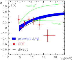
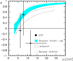
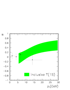
Figure 23: NRQCD calculation of $\alpha(p_{T})$ for (left) $J/\psi$ (Braaten et al.: Ref. Braaten:1999qk), (middle) $\psi^{\prime}$ (Leibovich: Ref. Leibovich:1996pa; Braaten et al.: Ref. Braaten:1999qk; Beneke et al.: Ref. Beneke:1996yw) and (right) $\Upsilon(1S)$ (Braaten-Lee: Ref. Braaten:2000gw).(left reprinted figure from Ref. Braaten:1999qk with permission of American Physical Society. Copyright (2000); from Ref. Braaten:1999qk, middle and right from Ref. yr)

In Fig. 23, we show the various polarisation calculations from NRQCD for prompt $J/\psi$, direct $\psi^{\prime}$ and $\Upsilon(1S)$ with feed-down from higher bottomonium taken into account. The least that we may say is that NRQCD through gluon fragmentation is not able to describe the present data on polarisation, especially if the trend to have $\alpha\leq 0$ at high $p_{T}$ is confirmed by future measurements.

Motivated by an apparent discrepancy in the hierarchy of the LDME’s for $J/\psi$ and $\psi^{\prime}$, Fleming, Rothstein and Leibovich[100] proposed different scaling rules belonging to NRQCD_c. Their prediction for the cross-section was equally good and for polarisation they predicted that $\alpha$ be close to $1/3$ at large $p_{T}$.

This latter proposal nevertheless raises some questions since the very utility of the scaling rules was to provide us with the evolution of the unknown matrix elements of NRQCD when the quark velocity $v$ changes, equally when one goes from one quarkonium family to another. Indeed, a LMDE scaling as ${\cal O}(v^{4})$ may be bigger than another scaling as ${\cal O}(v^{3})$ since we have no control on the coefficient multiplying the $v$ dependence. On the other hand, a comparison of the same LDME for a charmonium and the corresponding bottomonium is licit. Now, if the counting rules are modified between charmonia and bottomonia, the enhancement of the predictive power due to this scaling rules is likely to be reduced to saying that the unknown coefficient should not be that large and an operator scaling as ${\cal O}(v^{4})$ is conceivably suppressed to one scaling as ${\cal O}(v^{3})$, not more than a supposition then.

3.3 $k_{T}$ factorisation and BFKL vertex

If one considers the production of charmonium or bottomonium at hadron colliders such that the Tevatron, for reasonable values of $p_{T}$ and of the rapidity $y$, it can be initiated by partons with momentum as low as a few percent of that of the colliding hadrons. In other words, we are dealing with processes in the low Bjorken $x$ region. In that region we usually deal with the BFKL equation, which arises from the resummation of $\alpha_{s}\log(1/x)$ factors in the partonic distributions. This process of resummation involves what we can call Balitsky-Fadin-Kuraev-Lipatov (BFKL) effective vertices and the latter can be used in other processes than the evolution of parton distributions.

On the other hand, the $k_{T}$ factorisation approach[101, 102, 103, 104, 105, 106], which generalises the collinear approach to nonvanishing transverse momenta for the initial partons, can be coupled to the NLLA vertex to describe production processes, such as those of heavy quark or even quarkonium.

This combination of the $k_{T}$ factorisation for the initial partons and the NLLA BFKL effective vertex[107] for the hard part can be thought as the natural framework to deal with low $x$ processes since its approximations are especially valid in this kinematical region. As an example, very large contributions from NLO in the collinear factorisation are already included in the LO contributions of this approach. A typical case is the fragmentation processes at large $p_{T}$ in quarkonium production.

Since this approach is thought to be valid for low $x$ processes, but still at a partonic scale above $\Lambda_{\rm QCD}$, this can be also referred to as the semi-hard approach. One can find an useful review about the approach, its applications and its open questions in the two following papers of the small-x collaboration[108, 109].

3.3.1 Differences with the collinear approach

Practically, compared to the collinear approach, we can highlight two main differences. First, instead of appealing to collinear parton distributions, we are going to employ the unintegrated PDF ${\cal F}(x,{\bf q}_{T})$ for which there exist different parameterisations, exactly as for the collinear case. The discussion of the difference between these is beyond the scope of this review.

These are however related to the usual PDF’s by:

$$\begin{split}xg(x,\mu^{2})=\int^{\mu^{2}}_{0}\frac{d{\bf q}_{T}^{2}}{{\bf q}_{T}^{2}}{\cal F}(x,{\bf q}_{T}).\end{split}$$ (31)

Secondly, the hard part of the process is computed thanks to effective vertices derived in Ref. Fadin:1996nw or following the usual Feynman rules of pQCD using an extended set of diagram[110] due to the off-shellness of the $t$-channel gluons and then using what is called the Collins-Ellis “trick”[103] which consists in the following replacement: $\overline{\epsilon^{\mu}(q_{i})\epsilon^{\star\nu}(q_{i})}=\frac{q_{iT}^{\mu}q_{iT}^{\nu}}{|q_{iT}|^{2}}$. Let us present here the first approach and give the expression for the $Q\bar{Q}$ production vertex ${\cal V}$[111]:

$${\cal V}^{ab}=-g_{1}g_{2}u(k_{1})\left(T^{a}T^{b}\,{\cal B}(q_{1},q_{2},k_{1},k_{2})-T^{b}T^{a}{\cal B}^{T}(q_{1},q_{2},k_{2},k_{1})\right)\bar{v}(k_{2}),$$ (32)

where $a$, $b$ are the gluon colour indices, $T^{c}=\frac{1}{2}\lambda^{c}$, $k_{1}$, $k_{2}$ the (on-shell) heavy-quark and antiquark momenta, $q_{1}$, $q_{2}$, the (off-shell) gluon momentum, and $g_{1}$, $g_{2}$ the strong coupling constant which is evaluated at two different scales, $q_{1}^{2}$ and $q_{2}^{2}$ respectively. The expression for ${\cal B}(q_{1},q_{2},k_{1},k_{2})$ (and ${\cal B}^{T}$) is a sum of two terms

$$\begin{split}&{\cal B}(q_{1},q_{2},k_{1},k_{2})=\gamma^{-}\frac{q\!\!\!/_{1\perp}-k\!\!\!/_{1\perp}-m}{(q_{1}-k_{1})^{2}-m^{2}}\gamma^{+}-\frac{\gamma_{\beta}\Gamma^{+\,-\,\beta}(q_{2},q_{1})}{(k_{1}+k_{2})^{2}}\,,\\ &\left({\cal B}^{T}(q_{1},q_{2},k_{2},k_{1})=\gamma^{+}\frac{q\!\!\!/_{1\perp}-k\!\!\!/_{2\perp}+m}{(q_{1}-k_{2})^{2}-m^{2}}\gamma^{-}-\frac{\gamma_{\beta}\Gamma^{+\,-\,\beta}(q_{2},q_{1})}{(k_{1}+k_{2})^{2}}\right).\end{split}$$ (33)

where $\Gamma^{+\,-\,\beta}(q_{2},q_{1})=2(q_{1}-q_{2})^{\beta}-2q_{1}^{+}n^{-\beta}+2q_{2}^{-}n^{+\beta}-2q_{1}^{2}\,\frac{n^{-\beta}}{q_{1}^{-}+q_{2}^{-}}+2q_{2}^{2}\,\frac{n^{+\beta}}{q_{1}^{+}+q_{2}^{+}}$.

The first corresponds to the contribution of B in Fig. 24; the second, with an $\frac{1}{s}$ propagator, is linked to a transition between two (off-shell) $t$-channel gluons (Reggeons) and a (off-shell) gluon which subsequently splits into the heavy quark (C in Fig. 24).

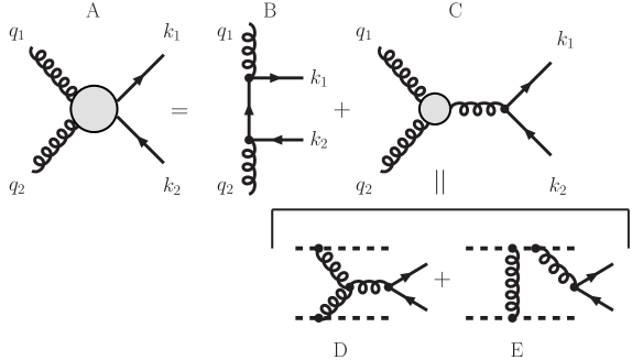
Figure 24: Different components in the $Q\bar{Q}$ production BFKL vertex.

This term is not only derived from a triple gluon vertex (D of Fig. 24). The complication is expected since the gluons are off-shell. Indeed if we want to deal with on-shell particles to impose current conservation, we have to go back to the particles –here the initial hadrons– which have emitted these $t$-channel gluons. Those can directly emit the third gluon in addition to the $t$-channel gluon (E of Fig. 24), similarly to a Bremßtrahlung contribution. This kind of emission gives birth to the two terms: $-2q_{1}^{2}\,\frac{n^{-\beta}}{q_{1}^{-}+q_{2}^{-}}+2q_{2}^{2}\,\frac{n^{+\beta}}{q_{1}^{+}+q_{2}^{+}}$. The factors $q_{1}^{2}$ and $q_{2}^{2}$ account for the fact that there is only one $t$-channel gluon in this type of process, the denominator comes from the propagator of the particle which has emitted the $s$-channel gluon.

The vertex of Eq. (LABEL:eq:BFKL_NNLA_vertex_QQ) has been used successfully for the description of open beauty production[111] and was also shown to give a large contribution to the production of $\chi_{c1}$ in the Colour-Singlet approach[112].

In the case of $\psi$ and $\Upsilon$ production in the Colour-Singlet approach, we need to consider the vertex $g^{\star}g^{\star}\to Q\bar{Q}g$ rather than $g^{\star}g^{\star}\to Q\bar{Q}$ to conserve $C$-parity. This would correspond to NNLLA corrections and these are not known yet. However, the reason of this complication ($C$-parity) is also from where one finds the solution since it sets the contributions of the unknown diagrams to zero when projected on a colour-singlet ${}^{3}S_{1}$ $Q\bar{Q}$ state. The expressions are finally the same with the addition of one gluon emission on the quark lines (see Ref. Hagler:2000eu).

The cross section is then obtained after the integration on the transverse momentum of the gluons and on the final state momenta ($P$ is the quarkonium momentum, $k$ that of the final state gluon). As in the usual CSM, the heavy-quark pair is projected on a colour-singlet ${}^{3}S_{1}$ state and their relative momentum is set to zero ($k_{1}=k_{2}$ and $P=k_{1}+k_{2}$). This gives

$$\begin{split}\sigma_{P_{1}P_{2}\to{\cal Q}gX}=\frac{1}{16(2\pi)^{4}}\frac{1}{8^{2}}\int\frac{d^{3}P}{P^{+}}\frac{d^{3}k}{k^{+}}d^{2}\vec{q}_{1T}d^{2}\vec{q}_{2T}&\delta^{2}(\vec{q}_{1T}-\vec{q}_{2T}-\vec{k}_{1T}-\vec{k}_{2T})\times\\ &\times\frac{{\cal F}(x_{1},\vec{q}_{1T})}{(q^{2}_{1T})^{2}}\frac{{\cal F}(x_{1},\vec{q}_{2T})}{(q^{2}_{2T})^{2}}\left|{\cal M}\right|^{2},\end{split}$$ (34)

where – $a$ and $b$ being the colour indices of the $t$-channel gluons, $i$ and $j$ those of the heavy quarks ($\left\langle 3i,\bar{3}j|1\right\rangle=\frac{\delta^{ij}}{\sqrt{3}}$) and ${\cal R}(0)$ the radial part of the Schrödinger wave function at the origin (in position space) –

$$\begin{split}{\cal M}^{ab}=\sum_{i,j}\sum_{L_{z},S_{z}}\frac{1}{\sqrt{m}}&\left\langle 0,0;1,S_{z}|1,J_{z}\right\rangle\left\langle 3i,\bar{3}j|1\right\rangle\frac{{\cal R}(0)}{\sqrt{4\pi}}\times\\ &\times{\rm Tr}\left(\frac{\epsilon\!\!\!/(S_{z})(k\!\!\!/_{1}+m)}{\sqrt{M}}{\cal V}_{Q_{i}\bar{Q}_{j}g}^{ab}(q_{1},q_{2},k_{1},k_{2}=k_{1},k)\right).\end{split}$$ (35)

Different projections can be used if one studies other quarkonia than the ${}^{3}S_{1}$. This formalism can be also combined with the COM by projecting the heavy-quark pair on a colour-octet state and introducing a LDME to give the probability for the non-perturbative transition into the physical quarkonium, exactly as in the collinear approach presented in section 3.2. Of course, as we shall see in the results, these LDME’s will have modified values compared to the ones of the collinear fits.

3.3.2 Results for $J/\psi$, $\psi^{\prime}$ and $\Upsilon(1S)$

Let us first present the result of Hägler et al.[113] who have used the KMS unintegrated PDF[114]. Since the hard part of the process is modified compared to the collinear case, it is not surprising that the ratio $k$ of the cross section of ${}^{1}\!S^{(8)}_{0}$ and ${}^{3}\!P^{(8)}_{0}$ is different, the slopes are still similar, though; an independent fit would not again distinguish the two LDME’s associated with these processes. The ratio $k$ lies between 6 at low $P_{T}$ and 4.5 and high $P_{T}$. They did the fit with these two contributions alone; their results are given in Table. 3.3.2. The first combination (only ${}^{1}S^{(8)}_{0}$) is plotted in Fig. 25.

Same as Table. 3.2.1 for $J/\psi$ production in the $k_{T}$ factorisation approach and the NLLA BFKL vertex. Values are given in units $10^{-2}$ GeV³. $\footnotesize\begin{array}[]{|c||c|c|c|c|c|c|}\hline\cr\mbox{}&{\mbox{PDF}}&\langle{\cal{O}}^{J/\psi}[{}^{3}S^{(8)}_{1}]\rangle&M_{k}^{J/\psi}({}^{1}S^{(8)}_{0},{}^{3}P^{(8)}_{0})&k&\\ \hline\cr\hline\cr\mbox{H\"{a}gler {et al.}~{}1}&{\mbox{KMS Ref.~{}\refcite{Kwiecinski:1997ee}}}&0.032\pm 0.012&7.0\pm 0.5&5&\mbox{only}^{1}S^{8}_{0}\\ \hline\cr\mbox{H\"{a}gler {et al.}~{}2}&{\mbox{KMS Ref.~{}\refcite{Kwiecinski:1997ee}}}&0.05\pm 0.012&6\pm 0.5&5&\mbox{only}^{3}P^{8}_{J}\\ \hline\cr\end{array}$

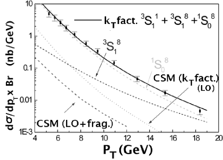
Figure 25: $J/\psi$ production cross sections at $\sqrt{s}=1.8$ TeV for the CSM in the collinear approach (LO + fragmentation), in the $k_{T}$ factorisation approach for the Colour-Singlet contribution and the Colour-Octet (${}^{3}S_{1}^{(8)}$ and ${}^{1}S_{0}^{(8)}$) compared to the direct measurement of CDF [49] (Reprinted figure from Ref. Hagler:2000eu with permission of American Physical Society. Copyright (2001)).

To what concerns the colour-singlet contribution, as can be seen on Fig. 25, it is more than one order of magnitude larger than the LO CSM contribution, and also larger than fragmentation-CSM contribution. The same trend is confirmed by the $\psi^{\prime}$ case[115]. This can be partially explained (up to a factor 2.5) by a genuine different choice for the scale at which $\alpha_{s}$ should be evaluated (cf. the factors $g_{1}$ and $g_{2}$ in Eq. (32)).

On the other hand, the colour-octet LDME $\langle{\cal{O}}^{J/\psi}[{}^{3}S^{(8)}_{1}]\rangle$ is thirty times smaller than in the collinear fits (compare Table. 3.2.1 and Table. 3.3.2) whereas $M_{k}^{J/\psi}({}^{1}S^{(8)}_{0},{}^{3}P^{(8)}_{0})$ is similar. In Ref. Hagler:2000eu, it is however emphasised that $\langle{\cal{O}}^{J/\psi}[{}^{3}S^{(8)}_{1}]\rangle=0$ would give a much worse fit, whereas, according to Baranov[110], $\langle{\cal{O}}^{J/\psi}[{}^{3}S^{(8)}_{1}]\rangle$ can be set to 0 with the unintegrated PDF of Ref. Blumlein:1995eu. The latter analysis of Baranov is dominated by the Colour-Singlet contribution and due to the longitudinal polarisation of the initial off-shell gluons[117], the polarisation parameter $\alpha$ should be negative and close to -1 as soon as $P_{T}$ reaches 6 GeV both for $J/\psi$ and $\psi^{\prime}$. The same results for $J/\psi$ and $\psi^{\prime}$ as presented in Fig. 3 of Ref. Yuan:2000qe are irrelevant since they do not take into account the weights of the different contributions in the particle yield. The polarisation of the quarkonia from isolated colour-octet channels is not measurable and it is obvious from the cross-section plots (Fig. 1 and Fig. 2 of Ref. Yuan:2000qe) that none of the colour-octet channels can reproduce the cross section alone, they should be combined.

To conclude this section, let us mention the combination of the $k_{T}$ factorisation approach with the colour-octet gluon fragmentation by Saleev et al.[119]. The hard part which is considered is $g^{*}g^{*}\to g$ where the $g^{*}$ are reggeised gluons (again distributed according to an unintegrated PDF) and where the gluon, $g$, subsequently fragments into a quarkonium via the colour-octet state ${}^{3}S_{1}^{(8)}$, exactly like in the collinear approach. The LDME values used were the one from the collinear fit[94] (see Table. 3.2.1) : $\langle{\cal{O}}^{J/\psi}[{}^{3}S^{(8)}_{1}]\rangle=0.44\times 10^{-2}$ GeV³ and $\langle{\cal{O}}^{\psi^{\prime}}[{}^{3}S^{(8)}_{1}]\rangle=0.42\times 10^{-2}$ GeV³. The agreement is reasonable contrasting with the conclusion from the LO $k_{T}$ factorisation analysis of Hägler et al.[113] which requires a strong suppression of the ${}^{3}S^{(8)}_{1}$ channel.

3.4 Durham group: enhanced NNLO contributions

As already said, ${}^{3}S_{1}$ quarkonia produced by gluon fusion are necessarily accompanied by a third gluon in the final state. Indeed, it is required for $C$-parity conservation and in the case of semi-inclusive reaction, as the ones we have been considering so far, this gluon cannot come from the initial states (see Fig. 26 (left)).

As we have seen, the classical description –through the CSM– of this kind of production (especially at LO) in QCD severely underestimates the production rates as measured at the Tevatron and even at RHIC. In their work[120], V.A. Khoze et al. considered the special case where this third gluon, attached to the heavy-quark loop, couples to another parton of the colliding hadrons and produces the gluon needed in the final state. Indeed, it is likely that the large number of possible graphs –due to the large number of available gluons at large $s$– may compensate the $\alpha_{s}$ suppression. The parton multiplicity $n$ behaves like $\log s$ and this process (see Fig. 26 (right)) can be considered as the LO amplitude in the BFKL approach whereas it is NNLO in pQCD.

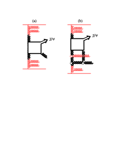
Figure 26: (left) Usual LO pQCD in the CSM; (right) NNLO pQCD or LO BFKL contributions. In both cases, the $gg\to{\cal Q}g$ sub-process is shown in bold and the two quarks entering the $\cal Q$ are on-shell.

3.4.1 Integrated cross section

Since the two $t$-channel gluon off the quark loop are now in a colour-octet symmetric state, the real part of the amplitude is expected to dominated by its imaginary part (in Fig. 26 (right) the two quarks and the gluon is the $s$-channel are then put on-shell as well as the remaining quark entering the $\cal Q$). One then chooses to work in the region where the rapidity between the $\cal Q$ and the final gluon $p$ is large (i.e. when $\hat{s}\gg M_{\cal Q}$) since it should dominate and one gets[120] the following expressions for the imaginary part of the amplitude for the two possible Feynman graphs (the two other ones with the loop momentum reverted give a factor two):

$$\begin{split}\Im mA^{a}=&\frac{3}{8}d^{abc}g(4\pi\alpha_{s})^{5/2}\times\\ \times&\int d\ell_{T}^{2}\frac{{\rm Tr}(\varepsilon\!\!\!/(p_{1})(\frac{P\!\!\!\!/}{2}+m_{Q})\varepsilon\!\!\!/(P)p\!\!\!/_{2}(\frac{-P\!\!\!\!/}{2}-\ell\!\!\!/+m_{Q})p\!\!\!/_{2}(\frac{P\!\!\!\!/}{2}-p\!\!\!/_{1}+m_{Q}))}{2\pi\hat{s}((\frac{P}{2}-p_{1})^{2}-m_{Q}^{2})(\ell^{2}-\lambda_{g}^{2})((q+\ell)^{2}-\lambda_{g}^{2})}\end{split}$$ (36)

$$\begin{split}\Im mA^{b}=&-\frac{3}{8}d^{abc}g(4\pi\alpha_{s})^{5/2}\times\\ \times&\int d\ell_{T}^{2}\frac{{\rm Tr}(\varepsilon\!\!\!/(p_{1})(\frac{P\!\!\!\!/}{2}-\ell+m_{Q})p\!\!\!/_{2}(\frac{-P\!\!\!\!/}{2}+m_{Q})\varepsilon\!\!\!/(P)p\!\!\!/_{2}(\frac{P\!\!\!\!/}{2}-\ell-p\!\!\!/_{1}+m_{Q}))}{2\pi\hat{s}((\frac{P}{2}-\ell-p_{1})^{2}-m_{Q}^{2})(\ell^{2}-\lambda_{g}^{2})((q+\ell)^{2}-\lambda_{g}^{2})},\end{split}$$ (37)

$g$ is a quantity related, up to some known factors, to $|\psi(0)|^{2}$ through the leptonic decay width ($g^{2}=\frac{3\Gamma_{\ell\ell}M_{\cal Q}}{64\pi\alpha_{QED}^{2}}$) such that the ${}^{3}S_{1}$ vertex reads $\frac{g}{2}(P\!\!\!\!/+M_{\cal Q})\varepsilon^{*}(P)$. $\lambda_{g}$ is an effective gluon mass to avoid logarithmic infrared singularity, motivated by possible confinement effects.

The partonic differential cross section thus reads:

$$\begin{split}\frac{d\hat{\sigma}}{dP^{2}_{T}}=\frac{|A|^{2}}{16\pi\hat{s}^{2}},\end{split}$$ (38)

with $A=2(A^{a}+A^{b})$. The hadronic cross section is obtained with the help of

$$\begin{split}\frac{d\sigma}{dydP^{2}_{T}}=\int\frac{dx_{2}}{x_{2}}x_{1}g(x_{1})x_{2}g(x_{2})\frac{d\hat{\sigma}(\hat{s},P^{2}_{T})}{dP^{2}_{T}},\end{split}$$ (39)

$\hat{s}=sx_{1}x_{2}$ with $\sqrt{s}$ the collision energy in the hadronic frame, $y$ is the rapidity of the $\cal Q$ also in the latter frame, $g(x_{i})$ are the gluon PDF.

Due to the low-$x$ behaviour of the PDF, the main contribution to the integral comes from the lowest value of $x_{2}$, that is $x_{2}\simeq\frac{\sqrt{M^{2}_{\cal Q}+P^{2}_{T}}}{\sqrt{s}}e^{-y}$ (and thus $x_{1}\simeq\frac{\sqrt{M^{2}_{\cal Q}+P^{2}_{T}}}{\sqrt{s}}e^{y}$). For reasons exposed in Ref. Khoze:2004eu, the $x_{2}$-integration region is to be extended over the whole kinematically available rapidity interval $\Delta y$, this gives

$$\begin{split}\frac{d\sigma}{dydP^{2}_{T}}=x_{1}(y)g(x_{1}(y))x_{2}(y)g(x_{2}(y))\Delta y\frac{d\hat{\sigma}(\hat{s}(x_{1},x_{2}),P^{2}_{T})}{dP^{2}_{T}},\end{split}$$ (40)

with $x_{1,2}(y)=\frac{\sqrt{M^{2}_{\cal Q}+P^{2}_{T}}}{\sqrt{s}}e^{\pm y}$ and

$$\begin{split}\Delta y=\ln(\frac{x^{2}_{max}s}{M^{2}_{\cal Q}+P^{2}_{T}}),\end{split}$$ (41)

with $x_{max}$ set to 0.3 to exclude contributions when the third gluon couples to partons with $x>0.3$ – this would have normally been suppressed by the PDF in conventional calculations. See Ref. Khoze:2004eu for further discussion about uncertainties linked to those approximations. Integrating over $P_{T}$, for $\sqrt{s}=1.96$ TeV with the LO MRST2001 gluon PDF[121] at the scale $\mu=0.5\sqrt{M^{2}_{\cal Q}+P^{2}_{T}}$, for $|y|<0.6$ and $\lambda_{g}=0.8$ GeV, the integrated cross section is

$$\begin{split}\sigma\simeq 2.7\mu b.\end{split}$$ (42)

This seems in agreement with the latest measurement by CDF[54] at $\sqrt{s}=1.96$ TeV in the whole $P_{T}$ range but for the total cross section only; the extraction of the prompt signal was only done for $P_{T}>1.25$ GeV.

As exposed in Ref. Khoze:2004eu, this calculation is affected by the following uncertainties:

1. Choice of the effective gluon mass, $\lambda_{g}$: for $\lambda_{g}=0.5,0.8,1.0$ GeV, $\sigma$ is 2.0, 2.7, 4.0 $\mu b$;

2. Choice of the factorisation $\mu_{F}$ scale (at which the PDF are evaluated) and renormalisation $\mu_{R}$ scale (at which $\alpha_{s}$ is evaluated): defining $\mu_{0}=\sqrt{M^{2}_{\cal Q}+P^{2}_{T}}$, setting $\mu_{F}=\mu_{R}$ to $0.5\,\mu_{0}$, $\mu_{0}$, $2\,\mu_{0}$, $\sigma$ is 2.7, 2.3, 1.5 $\mu b$;

3. Choice of the cut-off $x_{max}$: its variation introduces NLL corrections in the BFKL approach.

Beside those, we have the usual uncertainties linked to the PDF (especially at low $x$) and a possible $K$-factor or equally higher-order pQCD corrections.

Using the same parameters and setting $y=0$, one can in turn compute the cross sections for $\psi(2S)$, but also for $\Upsilon(nS)$ at $\sqrt{s}=1.96$ TeV and at $\sqrt{s}=14$ TeV (see Table 18).

Direct cross section calculations Ref. Khoze:2004eu. $\left.d\sigma/dy\right|_{y=0}$ $J/\psi$ ($\mu b$) $\psi(2S)$ ($\mu b$) $\Upsilon(1S)$ ($nb$) $\Upsilon(2S)$ ($nb$) $\Upsilon(3S)$ ($nb$) $\sqrt{s}=1.96$ TeV 2.2 0.6 40 12 9 $\sqrt{s}=14$ TeV 8.1 2.5 310 100 80

3.4.2 $P_{T}$ differential cross section

Unfortunately, one cannot rely on the amplitude written above the compute the $P_{T}$ differential cross section (see Ref. Khoze:2004eu). As a makeshift, they use a simple parameterisation for the partonic cross section based on dimensional counting:

$$\begin{split}\frac{d\hat{\sigma}}{dP^{2}_{T}}\propto g^{2}\alpha^{5}_{s}\frac{\ln\left(\frac{x^{2}_{max}s}{M^{2}_{\cal Q}+P^{2}_{T}}\right)}{(M^{2}_{\cal Q}+P^{2}_{T})^{3}}.\end{split}$$ (43)

Taking again $x_{max}=0.3$ and normalising the distribution by equating its integral over $P^{2}_{T}$ to the previous one, one obtains a reasonable agreement with the data from CDF. Again, the comparison is somewhat awkward since their prediction (for $\sqrt{s}=1.96$ TeV) is only for direct production (what they call “prompt”) whereas the data at $\sqrt{s}=1.96$ TeV are still only for prompt (and for $P_{T}>1.25$ GeV only).

3.4.3 Other results

Since some NNLO processes seem to have enhanced contributions, a second class of diagrams was considered where the two $t$-channel gluons “belong to two different pomerons”, or two different partons showers. This kind of contributions can be related to the single diffractive cross section (see Ref. Khoze:2004eu). It was however found that this class of diagrams contributes less that the one considered above, though it may compete with it at large $\sqrt{s}$.

In the same fashion, they consider associative production ${\cal Q}+c\bar{c}$, for which they expect $\hat{\sigma}(\psi c\bar{c})$ to be close to 2 $nb$, which gives for the hadronic cross section[120]:

$$\begin{split}\left.\frac{d\sigma(\psi c\bar{c})}{dy}\right|_{y=0}=x_{1}g(x_{1})x_{2}g(x_{2})\hat{\sigma}(\psi c\bar{c})\approx 0.05\mu b.\end{split}$$ (44)

In this case, it is about only 1 % of the other contributions.

3.5 CES: Comover Enhancement Scenario

3.5.1 General statements

In their model[122, 123], P. Hoyer and S. Peigné postulate the existence of a perturbative rescattering of the heavy-quark pair off a comoving colour field, which arises from gluon radiations preceding the heavy-quark pair production. The model is first developed for low $P_{T}\lesssim m$ production [122], and generalised in a second work[123], to large $P_{T}\gg m$, where quarkonium production is dominated by fragmentation. In general (i.e. at low and large $P_{T}$), the model assumes a rich colour environment in the fragmentation region of any (coloured) parton, modelled as a comoving colour field. In the case of large-$P_{T}$ production, the comoving field is assumed to be produced by the fragmenting parton DGLAP radiation. The strength and precise shape of the comoving field are not required to be the same at small and large $P_{T}$.

If, as they suppose, the presence of the comoving field is responsible for an enhancement of the production cross section, as it is absent in photon-hadron collisions (no colour radiation from the photon and no fragmentation in the $P_{T}$ region where the data are taken) there would not be any increase in photo-production. Indeed, the NLO CSM cross section[124] fits well the data and no modification is needed.

Taking benefit of this assumed perturbative character of the scattering and assuming simple properties of the comoving colour field – namely a classical isotropic colour field –, they are able to carry out the calculation of the rescattering, even when two rescatterings of the heavy-quark pair are required, as in the gluon fragmentation case[123], to produce a colour-singlet ${}^{3}S_{1}$ state. In the latter case, which is relevant at large transverse momentum, the $\psi^{\prime}$ (as well as directly produced $J/\psi$) is predicted to be produced unpolarised.

Another assumption, motivated by the consideration of the relevant time scales, is that the heavy quarks propagate nearly on-shell both before and after the rescattering. In the latter case, the assumption is comparable to the static approximation of the CSM. Furthermore, the rescattered quark pair is projected on a colour-singlet state which has the same spin state as the considered $\cal Q$, similarly to the CSM.

Note that since the strength of the field is unknown, only cross-section ratios and polarisations can be predicted in the framework of this model, not absolute normalisations. Let us review the high-$P_{T}$ case[123] which interests us most.

3.5.2 Results of the model

Considering two perturbative scatterings as illustrated in Fig. 27 and working in a first order approximation for quantities like $\frac{\vec{\ell}_{i}}{m}$ and $\frac{\vec{q}}{m}$ for on-shell quarks before and after the rescattering, they show[123] that the rescattering amplitude to form a colour-singlet ${}^{3}S_{1}$ quarkonium from a gluon can be cast in the following simple form:

$${\cal M}(^{3}S_{1},S_{z})=\frac{-{\cal R}(0)g_{s}^{3}}{2\sqrt{6\pi m^{3}}}\,d_{ab_{1}b_{2}}\vec{G}_{1}\cdot\vec{\varepsilon}(\lambda_{g})\,\vec{G}_{2}\cdot\vec{\varepsilon}(S_{z})^{*},$$ (45)

where $\lambda_{g}$ is the polarisation of the fragmenting gluon, $\vec{G}_{i}=\vec{\Gamma}_{f}(\vec{\ell}_{i})\times\vec{\ell}_{i}$ involves the colour field $\Gamma_{f}$ produced by the fragmentation, $\ell_{1}$ and $\ell_{2}$ are –as depicted in Fig. 27– the momenta of the two rescattering gluons. As usual, ${\cal R}(0)$ is the radial wave function at origin. Apart from the presence of rescatterings, their approach follows the same lines as the CSM with a projection on static colour-singlet states with the proper spin state.

Very interesting pieces of information can be extracted from this formula: since Eq. (45) is independent of $\Gamma_{f}^{0}$, solely transverse gluons emerging from the comoving gluon field contribute to ${}^{3}S_{1}$ quarkonium production at high $P_{T}$. Gauge invariance is also preserved: ${\cal M}(\Gamma_{f}^{\mu}(\ell_{i})\to\ell_{i}^{\mu})=0$ since the quarks are on-shell. Besides this, the most interesting part is the factorised dependence on the fragmenting gluon and quarkonium polarisations. They appear in two different scalar products with the quantity $\vec{G}$ involving the comoving field $\Gamma_{f}$. The polarisation of the quarkonium depends solely on the properties of the comoving field through $\vec{G}_{2}$.

This outcome of this perturbative calculation is totally at variance with the statement of Cho and Wise[97], i.e. a ${}^{3}S_{1}$ produced by a high $P_{T}$ (thus real and transverse) gluon is to be transversally polarised. More precisely, if the comoving field is supposed to be isotropically distributed in the comoving $Q\bar{Q}$ rest frame, then they predict an unpolarised production of ${}^{3}S_{1}$ quarkonia in the high $P_{T}$ region.

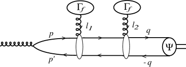
Figure 27: Rescattering scenario for a fragmenting gluon into a colour-singlet ${}^{3}S_{1}$ quarkonium.

To what concerns $P$-waves, they predict that “rather independently of the form of $\Gamma_{f}$”, $\chi_{1}$ should be “longitudinally polarised if the rescattering scenario dominates $\chi_{1}$ production at high $P_{T}$”. Finally, we should emphasise that the approach at high $P_{T}$ applies equally for charmonium and bottomonium as long as gluon fragmentation matters. This sole consideration of gluon fragmentation can be seen as a drawback: indeed $c$-quark fragmentation seems to be bigger than gluon one since it is one order of $\alpha_{s}$ less (see Fig. 7 (left)).

In conclusion, this simple production model seems quite interesting (and motivated by phenomenology [122]), even though the properties of this comoving field are poorly known (to obtain the results mentioned here, it was supposed to be classical and isotropically distributed in the $Q\bar{Q}$ rest frame). The existence of such perturbative reinteraction should be also searched for in other processes involving quarkonia. A qualitative agreement between the predictions of the model and future data on polarisation and cross-section ratios would be quite intriguing and might indicate the importance of comovers in quarkonium production.

3.6 Non-static and off-shell contributions to the CSM

As we have seen, none of the models reviewed above provides an entirely conclusive solution to the heavy-quarkonium production problem, especially without the introduction of new mechanisms and associated free parameters. Considering that the CSM is still the most natural way to describe heavy-quarkonium production, it is legitimate to wonder whether some of the hypotheses of this model were actually justified. One of these is in fact common to the CSM, the COM and the CES and can be referred to as the static approximation, in the sense that one considers the hard part of the process solely for configurations where the heavy quarks are on-shell and at rest in the frame of the quarkonium to be created.

This approximation is usually justified by the fact that the wave function, parameterising the amplitude of probability for the binding, should be peaked at the origin and expanding its product with the hard amplitude, one has only to keep the first non-vanishing term in the Taylor series. In the latter, the hard part is evaluated at this static and on-shell configuration.

This is legitimate as long as the hard part is “well-behaved”, e.g. does not present singularities in the non-static region. In order to test the validity of this supposition, one has to reconsider the basis of quarkonium ($\cal Q$) production in field theory. In the following, we review a consistent and systematic scheme to go beyond this static approximation proposed by J. P. Lansberg, J. R. Cudell and Y. L. Kalinovsky. In the latter scheme, when off-shell configurations are taken into account, there exist new contributions at the leading-order for ${}^{3}S_{1}$ production by gluon fusion. These can compete with the ones considered in the CSM.

This approach requires the use of 3-point vertices depending on the relative momentum of the constituent quarks of the $\cal Q$ which can be paralleled to Bethe-Salpeter vertex functions. The arbitrary normalisation of these is fixed by the calculation of the $\cal Q$ leptonic width. Gauge invariance, which could be spoilt by non-local contributions, is preserved by the introduction of 4-point vertices.

3.6.1 Description of the bound-state nature of the quarkonia

The transition $q\bar{q}\rightarrow{\mathcal{Q}}$ can be described by the following 3-point function[125, 81]:

$$\Gamma^{(3)}_{\mu}(p,P)=\Gamma(p,P)\gamma_{\mu},$$ (46)

with $P\equiv p_{1}-p_{2}$ the total momentum of the bound state, and $p\equiv(p_{1}+p_{2})/2$ the relative momentum of the bound quarks. This choice amounts to describing the vector meson as a massive photon with a non-local coupling and is justified by other studies (see e.g. Ref. Burden:1996nh).

In order to go beyond the static limit, the quarks are not supposed to be on-shell. To allow connections with wave functions, $\Gamma(p,P)$ is taken as a function of the square of the relative c.m. 3-momentum $\vec{p}$ of the quarks, which can be written in a Lorentz invariant form as $\vec{p}^{\,\,2}=-p^{2}+\frac{(p.P)^{2}}{M^{2}}$ and possible cuts in the vertex function $\Gamma(p,P)$ are neglected. Two opposite scenarios have been considered:

$$\begin{split}\Gamma(p,P)=\frac{N}{(1+\frac{\vec{p}^{\,2}}{\Lambda^{2}})^{2}}\text{ and }\Gamma(p,P)=Ne^{-\frac{\vec{p}^{\,2}}{\Lambda^{2}}},\end{split}$$ (47)

both with a normalisation $N$ and a size parameter $\Lambda$, which can be obtained from relativistic quark models[127, 128, 129, 130]. The normalisation $N$ can be fixed from the leptonic-decay width and the procedure to do so is thoroughly explained in[81, 131].

3.6.2 LO production diagrams

As usual, it is natural to think of gluon-fusion process to produce quarkonia at high-energy, especially if the value of $P_{T}$ is not excessively large. To conserve $C$ parity, in the case of ${}^{3}S_{1}$ production, a third gluon is required; this leads to the consideration of $gg\to{\cal Q}g$ processes.

As explained in Ref. Lansberg:2005pc, the use of the Landau equations to determine the discontinuities of the amplitude leads us to the distinction between two families of diagrams, the first is the one which gives the usual LO CSM contributions[27, 28, 29] when the relative momentum of the heavy quarks entering the ${\cal Q}$ is set to zero, the other family is absent in the on-shell limit and was never considered before Ref. Lansberg:2005pc in the case of ${\cal Q}$ inclusive production. These are shown in Fig. 28.

   

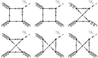
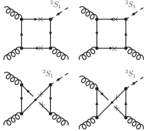
Figure 28: The first family (left) has 6 diagrams and the second family (right) has 4 diagrams contributing to the discontinuity of $gg\to\!\!\ ^{3}S_{1}g$ at LO in QCD.

3.6.3 Gauge invariance

Now, the diagrams of Fig. 28 (right) are not gauge invariant. Indeed, the vertex function $\Gamma(p,P)$ takes different values in diagrams where either the on-shell quark or the antiquark touches the $\cal Q$, so that current conservation is shattered compared to the case where the $\cal Q$ is replaced by a photon.

    

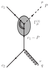
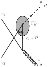
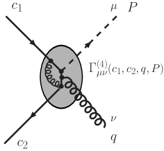
Figure 29: Illustration of the necessity of a 4-point vertex.

Physically, this can be understood by the lack of some diagrams: if one considers a local vertex, then the gluon can only couple to the quarks that enter it. For a non-local vertex, it is possible for the gluon to connect to the quark or gluon lines inside the vertex, as shown in Fig. 29. These contributions are related to a 4-point $q\bar{q}{\cal Q}g$ vertex, $\Gamma^{(4)}_{\mu\nu}(c_{1},c_{2},q,P)$, whose form is, in general, unknown, although it must obey some general constraints[125, 81, 132]:

• it must restore gauge invariance: its addition to the amplitude must lead to current conservation at the gluon vertex;

• it must obey crossing symmetry (or invariance by $C$ conjugation) which can be written

  $$\Gamma^{(4)}_{\mu\nu}(c_{1},c_{2},q,P,m)=-\gamma_{0}\Gamma_{\mu\nu}^{(4)}(-c_{2},-c_{1},q,P,-m)^{\dagger}\gamma_{0};$$ (48)

• it must not introduce new singularities absent from the propagators or from $\Gamma(p,P)$, hence it can only have denominators proportional to $(c_{1}-P)^{2}-m^{2}$ or $(c_{2}+P)^{2}-m^{2}$;

• it must vanish in the case of a local vertex $\Gamma_{\mu}^{(3)}\propto\gamma_{\mu}$, hence we multiply it by $\Gamma(2c_{1}-P,P)-\Gamma(2c_{2}+P,P)$.

These conditions are all fulfilled by the following simple choice[125]:

$$\Gamma^{(4)}_{\mu\nu}(c_{1},c_{2},P,q) = -ig_{s}T^{a}_{ki}\left[\Gamma(2c_{1}-P,P)-\Gamma(2c_{2}+P,P)\right]$$ (49)

$$\times \left[\frac{c_{1\nu}}{(c_{2}+P)^{2}-m^{2}}+\frac{c_{2\nu}}{(c_{1}-P)^{2}-m^{2}}\right]\gamma_{\mu}$$

where the indices of the colour matrix $T$ are defined in Fig. 30, and $g_{s}$ is the strong coupling constant.

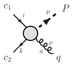
Figure 30: The gauge-invariance restoring vertex, $\Gamma^{(4)}$.

It should be also emphasised that this choice of vertex is not unique. A first study of the effect of different choices can be found in Ref. Lansberg:2005aw,Lansberg:2005gs, where we can see that agreement with data can be reached. The introduction of such new vertex can be paralleled with the COM since the quark pair $(c_{1},c_{2})$ that makes the meson is now in a colour-octet state. Such configurations are required here to restore gauge invariance.

This new $\Gamma^{(4)}$ vertex introduces two new diagrams in the calculation of the amplitude which, now, becomes a gauge-invariant quantity. The detail of the calculation of the polarised cross section can be found in Refs. Lansberg:2005pc,Lansberg:2005aw.

3.6.4 Results for $J/\psi$ and $\psi^{\prime}$

We show in Fig. 31 (left) the results obtained in Ref. Lansberg:2005pc for $\sqrt{s}=1800$ GeV, $|\eta|<0.6$, $m=1.87$ GeV and $\Lambda=1.8$ GeV. The curves for $\sigma_{TOT}$, $\sigma_{T}$ and $\sigma_{L}$ are calculated within this approach with the new cut only (see Ref. Lansberg:2005pc for details), the LO CSM is recalculated from the expression of Refs. CSM_hadron1,CSM_hadron2,CSM_hadron3.

In fact, the normalisation of the results using the decay width removes most dependence on the choice of parameters: instead of a factor 100 of difference expected from $\left(\frac{N_{\Lambda=1.0}}{N_{\Lambda=2.2}}\right)^{2}$ there is less than a factor 2 at $P_{T}=4$ GeV and a factor 3 at $P_{T}=20$ GeV. Interestingly, the dependence on $\Lambda$ is negligible once values of the order of 1.4 GeV are taken.

 

Figure 31: (left) Polarised ($\sigma_{T}$ and $\sigma_{L}$) and total ($\sigma_{TOT}$) cross sections obtained with a Gaussian vertex function, $m=1.87$ GeV, $\Lambda=1.8$ GeV and the MRST gluon distribution[121], to be compared with LO CSM. (right); Polarised ($\sigma_{T}$ and $\sigma_{L}$) and total ($\sigma_{TOT}$) cross sections for $\psi^{\prime}$ obtained with a Gaussian vertex function, $a_{node}=1.334$ GeV, $m=1.87$ GeV, $\Lambda=1.8$ GeV and the CTEQ gluon distribution [134], to be compared with LO CSM, CSM fragmentation[46, 42] and the data from CDFCDF7997a.

We see that the contribution of the new cut cannot be neglected at large $P_{T}$. It is interesting to see that it is much flatter in $P_{T}$ than the LO CSM, and its polarisation is mostly longitudinal. This could have been expected as scalar products of $\varepsilon_{L}$ with momenta in the loop will give an extra $\sqrt{\hat{s}}$ contribution, or equivalently an extra $P_{T}$ power in the amplitude, compared to scalar products involving $\varepsilon_{T}$.

Although the use of the leptonic width is a good means to fix most of the dependence on $N$ in the $J/\psi$ case, it is not so for radially excited states, such as the $\psi^{\prime}$. Indeed, in this case, the vertex function must have a node. We expect that $\Gamma_{2S}(p,P)$ should be well parametrised by

$$\begin{split}\left(1-\frac{|\vec{p}|}{a_{node}}\right)\frac{N^{\prime}}{(1+\frac{|\vec{p}|^{2}}{\Lambda^{2}})^{2}}\text{ or }N^{\prime}\left(1-\frac{|\vec{p}|}{a_{node}}\right)e^{\frac{-|\vec{p}|^{2}}{\Lambda^{2}}},\end{split}$$ (50)

where $a_{node}$ is the node position.

However, the position of the node is not very well-known, and it is not straightforward to relate our vertex with off-shell quarks to an on-shell non-relativistic wave function. Let us suppose here that the node has the same position in the vertex function than in the wave function: now, the integrand changes sign at $a_{node}$ and the positive contribution to the integral can be compensated by the negative one for a precise values of $a_{node}$; the latter turns out to be close to the estimated value of the node in the wave function. In other words, our normalisation procedure, translated from that of the CSM, gives a large value for $N$ compared to the $J/\psi$ case, whereas the calculation of the $\psi^{\prime}$ production amplitude is not affected much by the presence of a node in $\Gamma$.

Fig. 31 (right) shows that for $a_{node}=1.334$ GeV, one obtains a good fit to CDF data at moderate $P_{T}$ (note that the slopes are quite similar. This is at odds with what is commonly assumed since fragmentation processes –with a typical $1/P_{T}^{4}$ behaviour– can also describe the data). The $\psi^{\prime}$ is predicted to be mostly longitudinal.

In conclusion, the procedure followed by Lansberg et al. enables to go beyond the static approximation of the CSM by taking into account configurations where the quarks which form the quarkonium can have a nonzero relative momentum and can be off-shell. As one can see for radially excited states like $\psi^{\prime}$, very important effects can be omitted otherwise. Another important point raised is that new cut contributions can appear in this non-static extension. These have been computed and were shown to be at least non-negligible at high $P_{T}$. Indeed, there exist ambiguities in the way to preserve gauge-invariance and these might leave room for a better description of the data.

4 Conclusions and perspectives

In this review, we have tried to provide a wide overview about the problem of the hadroproduction of $J/\psi$, $\psi^{\prime}$, $\Upsilon(1S)$, $\Upsilon(2S)$ and $\Upsilon(3S)$. In order to clarify the discussion, we have limited ourselves to the study of direct production, which does not involve decays of higher excited states (like $P$-waves) nor of beauty hadron in the charmonium case.

On the experimental side, we benefit nowadays from studies from two hadron colliders, the Tevatron and RHIC. We have reviewed in detail the procedure used and the results obtained by the CDF collaboration. The situation is ideal for $\psi^{\prime}$ as they are able to extract the direct cross section as well as the polarisation measurement for the sole direct sample; for $J/\psi$ and $\Upsilon(1S)$, they have extracted the direct cross section and a polarisation measurement, including excited states contributions though; for $\Upsilon(2S)$, $\Upsilon(3S)$, solely the total cross section was measured. To what concerns the Run II, they are able to go to smaller $P_{T}$ but the direct signal as well as the polarisation measurement is still under study. Preliminary data nevertheless tend to show a confirmation that the (prompt) $J/\psi$ are in fact produced unpolarised if not longitudinal. This is in striking contradiction with all the NRQCD predictions. To what concerns RHIC collider, the PHENIX collaboration measured for the first time the $J/\psi$ cross section at $\sqrt{s}=200$ GeV where the non-prompt signal is negligible contrary to $\chi_{c}$ feed-down.

On the theoretical side, many models and calculations have been proposed since the outbreak of the $\psi^{\prime}$ anomaly in the mid-nineties. We have reviewed six of them. In order to present them on the same footage, we have limited ourselves to their basic points and their most important results.

We have first started with the Soft-Colour Interaction approach which deals with Monte Carlo simulation. It introduces the possibility of colour quantum-number exchanges between partons produced during the collision. This effectively opens a gluon fragmentation channel into ${}^{3}S_{1}$ at LO. The sole new parameter brought in is in fact kept at the same value as in the description of rapidity gaps but the approach is likely to suffer from some of the drawbacks as the Colour-Evaporation Model.

Secondly, we have reviewed the NRQCD factorisation approach, which is usually embedded, in hadroproduction, in the Colour-Octet Mechanism. We have presented the initial motivations of the approach, namely to cure IR divergences of the Colour-Singlet Model. Since it introduces unknown non-perturbative parameters called Long-Distance Matrix Elements (LDME), we have reproduced the values obtained by different groups, as well as the values obtained for the Colour-Singlet matrix elements. As said before, this approach is in contradiction with data to what concerns the polarisation. Some modifications of the scaling rules, which normally provide a hierarchy between the LMDE’s, were proposed to reduce the discrepancy but the confirmation of the new CDF preliminary measurement would certainly blacken the setting. Finally, according to a recent analysis centered on fixed-target experiments by F. Maltoni et al.[135] the universality of these LDME’s is far from being observed.

Thirdly, we have reviewed the application of the $k_{T}$ factorisation approach to hadroproduction. We have emphasised the two main differences with the collinear approaches (CSM or COM), namely the use of unintegrated PDF’s and of the effective BFKL vertices. As we have said, the LO contributions include naturally fragmentation channels; this lets us think that the approach is perhaps more suitable than the collinear ones. In the case of COM, we have given the values of the LDME’s obtained. These are smaller than the corresponding ones fit from the collinear cross sections and thus in better agreement with what is expected from $ep$ data from HERA[37] and perhaps also from fixed-target experiments[135].

Fourthly, we have briefly reviewed a calculation proposed by physicists from Durham of some specific NNLO pQCD contributions of the CSM. These can be viewed as LO BFKL contributions and thus are expected to be enhanced compared to other NNLO pQCD ones. Unfortunately, the method used cannot predict the $P_{T}$ slope of the cross section.

The fifth model reviewed deals with reinteractions with comovers. Two pictures were analysed: one for small $P_{T}$ events where the comovers are created by Bremßtrahlung of the colliding gluons and another for high-$P_{T}$ events where they are produced by DGLAP radiation of the fragmenting parton. The authors of the model suspect such re-scatterings to be source of a possible enhancement of the cross section, and if the picture holds, they predict that in the case of gluon fragmentation, the quarkonia are produced unpolarised.

The last approach reviewed is a consistent scheme to go beyond the static and on-shell approximation used, for instance, in the CSM and the CEM. The loss of gauge invariance caused by the introduction of such non-local effects was shown to be curable by the introduction of 4-point vertices. In the case of $\psi^{\prime}$, the presence of a node in the vertex function, which is typical of radially excited states and whose effects are necessarily neglected in the static approximation, was shown to have non-negligible effects and is therefore expected to be analysed in other processes.

Finally, on a more formal basis, for all models, we are lacking a factorisation theorem suitable both for charmonium and bottomonium cases. To what concerns NRQCD, even though some modification of it are required[137], it has been shown recently that the (modified) picture still holds at NNLO[136] at least for fragmentation processes which are supposed to dominate in the large $P_{T}$ regime.

In view of similar discrepancies between theory and data at $B$-factories, we strongly believe that the forthcoming efforts both on the experimental side and theoretical side will be fruitful and will certainly shed light on the interplay between the perturbative QCD and the bound-state physics for which quarkonium physics is archetypal.

References

- [1] J. J. Aubert et al. [E598 Collaboration], Phys. Rev. Lett. 33 (1974) 1404.
- [2] J. E. Augustin et al. [SLAC-SP-017 Collaboration], Phys. Rev. Lett. 33 (1974) 1406.
- [3] C. Bacci and et al., Phys. Rev. Lett. 33 (1974) 1408 [Erratum-ibid. 33 (1974) 1649].
- [4] W. Braunschweig et al. [DASP Collaboration], Phys. Lett. B 57 (1975) 407.
- [5] B. Richter, SLAC-PUB-1478 Plenary Session Report at XVII International Conference on High Energy Physics, London, Eng., Jul 1-10, 1974
- [6] J. D. Bjorken and S. L. Glashow, Phys. Lett. 11 (1964) 255.
- [7] S. L. Glashow, J. Iliopoulos and L. Maiani, Phys. Rev. D 2, (1970) 1285.
- [8] T. Appelquist, A. De Rujula, H. D. Politzer and S. L. Glashow, Phys. Rev. Lett. 34 (1975) 365.
- [9] G. Goldhaber et al., Phys. Rev. Lett. 37 (1976) 255.
- [10] J. Wiss et al., Phys. Rev. Lett. 37 (1976) 1531.
- [11] B. Knapp et al., Phys. Rev. Lett. 37, (1976) 882.
- [12] M. L. Perl et al., Phys. Rev. Lett. 35 (1975) 1489.
- [13] D. C. Hom et al., Phys. Rev. Lett. 36 (1976) 1236.
- [14] S. W. Herb et al., Phys. Rev. Lett. 39 (1977) 252.
- [15] W. R. Innes et al., Phys. Rev. Lett. 39 (1977) 1240 [Erratum-ibid. 39 (1977) 1640].
- [16] K. Ueno et al., Phys. Rev. Lett. 42 (1979) 486.
- [17] C. Bebek et al., Phys. Rev. Lett. 46 (1981) 84.
- [18] M. Basile et al., Lett. Nuovo Cim. 31 (1981) 97.
- [19] F. Abe et al. [CDF Collaboration], Phys. Rev. D 50 (1994) 2966.
- [20] F. Abe et al. [CDF Collaboration], Phys. Rev. Lett. 74 (1995) 2626 [arXiv:hep-ex/9503002].
- [21] S. Abachi et al. [D0 Collaboration], Phys. Rev. Lett. 74 (1995) 2632 [arXiv:hep-ex/9503003].
- [22] S. Eidelman et al. [Particle Data Group Collaboration], Phys. Lett. B 592 (2004) 1.
- [23] J. C. Collins, D. E. Soper and G. Sterman, Adv. Ser. Direct. High Energy Phys. 5 (1988) 1 [arXiv:hep-ph/0409313].
- [24] G. T. Bodwin, Phys. Rev. D 31 (1985) 2616 [Erratum-ibid. D 34 (1986) 3932].
- [25] J. w. Qiu and G. Sterman, Nucl. Phys. B 353 (1991) 105.
- [26] J. w. Qiu and G. Sterman, Nucl. Phys. B 353 (1991) 137.
- [27] C-H. Chang, Nucl. Phys. B 172 (1980) 425.
- [28] R. Baier and R. Rückl, Phys. Lett. B 102 (1981) 364.
- [29] R. Baier and R. Rückl, Z. Phys. C 19 (1983) 251.
- [30] E. L. Berger and D. L. Jones, Phys. Rev. D 23 (1981) 1521.
- [31] F. Halzen, F. Herzog, E. W. N. Glover and A. D. Martin, Phys. Rev. D 30 (1984) 700.
- [32] E. W. N. Glover, A. D. Martin and W. J. Stirling, Z. Phys. C 38 (1988) 473 [Erratum-ibid. C 49 (1991) 526].
- [33] H. Fritzsch, Phys. Lett. B 67 (1977) 217.
- [34] F. Halzen, Phys. Lett. B 69 (1977) 105.
- [35] J.F Amundson, O.J.P. Éboli, E.M. Gregores, F. Halzen, Phys. Lett. B 372 (1996) 127.
- [36] J.F Amundson et al., Phys. Lett. B 390 (1997) 323.
- [37] N. Brambilla et al., Heavy quarkonium physics, CERN Yellow Report, CERN-2005-005, 2005 Geneva : CERN, 487 pp [arXiv:hep-ph/0412158].
- [38] C. Albajar et al. [UA1 Collaboration], Phys. Lett. B 256 (1991) 112.
- [39] F. Abe et al. [CDF Collaboration], Phys. Rev. Lett. 69 (1992) 3704.
- [40] [CDF Collaboration], arXiv:hep-ex/9412013.
- [41] F. Abe et al. [CDF Collaboration], Phys. Rev. Lett. 79 (1997) 572.
- [42] E. Braaten, M. A. Doncheski, S. Fleming and M. L. Mangano, Phys. Lett. B 333 (1994) 548 [arXiv:hep-ph/9405407].
- [43] E. Braaten and T. C. Yuan, Phys. Rev. Lett. 71 (1993) 1673 [arXiv:hep-ph/9303205].
- [44] E. Braaten, K. m. Cheung and T. C. Yuan, Phys. Rev. D 48 (1993) 4230 [arXiv:hep-ph/9302307].
- [45] E. Braaten and T. C. Yuan, Phys. Rev. D 50 (1994) 3176 [arXiv:hep-ph/9403401].
- [46] M. Cacciari and M. Greco, Phys. Rev. Lett. 73 (1994) 1586 [arXiv:hep-ph/9405241].
- [47] G. Curci, W. Furmanski and R. Petronzio, Nucl. Phys. B 175 (1980) 27.
- [48] J. C. Collins and D. E. Soper, Nucl. Phys. B 194 (1982) 445.
- [49] F. Abe et al. [CDF Collaboration], Phys. Rev. Lett. 79 (1997) 578.
- [50] M. Kramer, Prog. Part. Nucl. Phys. 47 (2001) 141 [arXiv:hep-ph/0106120].
- [51] C. F. Qiao, J. Phys. G 29, 1075 (2003).
- [52] F. Abe et al. [CDF Collaboration], Phys. Rev. Lett. 71 (1993) 3421.
- [53] CDF Collab., http://www-cdf.fnal.gov/physics/new/bottom/cdf3124/cdf3124.html.
- [54] D. Acosta et al. [CDF Collaboration], Phys. Rev. D 71 (2005) 032001 [arXiv:hep-ex/0412071].
- [55] F. Abe et al. [CDF Collaboration], Phys. Rev. Lett. 75 (1995) 4358.
- [56] D. Acosta et al. [CDF Collaboration], Phys. Rev. Lett. 88 (2002) 161802.
- [57] T. Affolder et al. [CDF Collaboration], Phys. Rev. Lett. 84 (2000) 2094 [arXiv:hep-ex/9910025].
- [58] R. J. Cropp, FERMILAB-THESIS-2000-03.
- [59] T. Affolder et al. [CDF Collaboration], Phys. Rev. Lett. 85 (2000) 2886 [arXiv:hep-ex/0004027].
-
[60]
[CDF Collaboration], Note 05-04-28,
http://www-cdf.fnal.gov/physics/new/bottom/bottom.html - [61] S. S. Adler et al. [PHENIX Collaboration], Phys. Rev. Lett. 92 (2004) 051802 [arXiv:hep-ex/0307019].
- [62] G. C. Nayak, M. X. Liu and F. Cooper, Phys. Rev. D 68 (2003) 034003 [arXiv:hep-ph/0302095].
- [63] M. Klasen, B. A. Kniehl, L. N. Mihaila and M. Steinhauser, Phys. Rev. D 68 (2003) 034017 [arXiv:hep-ph/0306080].
- [64] A. Edin, G. Ingelman and J. Rathsman, Phys. Lett. B 366 (1996) 371 [arXiv:hep-ph/9508386].
- [65] A. Edin, G. Ingelman and J. Rathsman, Z. Phys. C 75 (1997) 57 [arXiv:hep-ph/9605281].
- [66] A. Edin, G. Ingelman and J. Rathsman, Phys. Rev. D 56 (1997) 7317 [arXiv:hep-ph/9705311].
- [67] J. Damet, G. Ingelman and C. B. Mariotto, JHEP 0209 (2002) 014 [arXiv:hep-ph/0111463].
- [68] C. B. Mariotto, M. B. Gay Ducati and G. Ingelman, Eur. Phys. J. C 23 (2002) 527 [arXiv:hep-ph/0111379].
- [69] T. Sjostrand, Comput. Phys. Commun. 82 (1994) 74.
- [70] S. Abachi et al. [D0 Collaboration], Phys. Lett. B 370 (1996) 239.
- [71] T. Affolder et al. [CDF Collaboration], Phys. Rev. Lett. 86 (2001) 3963.
- [72] R. Barbieri, R. Gatto and E. Remiddi, Phys. Lett. B 61 (1976) 465.
- [73] R. Barbieri, M. Caffo and E. Remiddi, Nucl. Phys. B 162 (1980) 220.
- [74] R. Barbieri, M. Caffo, R. Gatto and E. Remiddi, Phys. Lett. B 95 (1980) 93.
- [75] R. Barbieri, M. Caffo, R. Gatto and E. Remiddi, Nucl. Phys. B 192 (1981) 61.
- [76] W. E. Caswell and G. P. Lepage, Phys. Lett. B 167 (1986) 437.
- [77] G. T. Bodwin, E. Braaten and G. P. Lepage, Phys. Rev. D 51 (1995) 1125 [Erratum-ibid. D 55 (1997) 5853] [arXiv:hep-ph/9407339].
- [78] E. Braaten and S. Fleming, Phys. Rev. Lett. 74 (1995) 3327 [arXiv:hep-ph/9411365].
- [79] P. L. Cho and A. K. Leibovich, Phys. Rev. D 53 (1996) 150 [arXiv:hep-ph/9505329].
- [80] P. L. Cho and A. K. Leibovich, Phys. Rev. D 53 (1996) 6203 [arXiv:hep-ph/9511315].
- [81] J. P. Lansberg, Quarkonium Production at High-Energy Hadron Colliders, Ph.D. Thesis, Liège University, Belgium. ISBN: 2-87456-004-9 [arXiv:hep-ph/0507175].
- [82] B. Z. Kopeliovich and J. Raufeisen, Lect. Notes Phys. 647 (2004) 305 [arXiv:hep-ph/0305094].
- [83] W. Buchmuller, G. Grunberg and S. H. H. Tye, Phys. Rev. Lett. 45 (1980) 103 [Erratum-ibid. 45 (1980) 587].
- [84] W. Buchmuller and S. H. H. Tye, Phys. Rev. D 24 (1981) 132.
- [85] A. Martin, Phys. Lett. B 93 (1980) 338.
- [86] E. Eichten, K. Gottfried, T. Kinoshita, K. D. Lane and T. M. Yan, Phys. Rev. D 17 (1978) 3090 [Erratum-ibid. D 21 (1980) 313].
- [87] E. Eichten, K. Gottfried, T. Kinoshita, K. D. Lane and T. M. Yan, Phys. Rev. D 21 (1980) 203.
- [88] E. Braaten, S. Fleming and A. K. Leibovich, Phys. Rev. D 63 (2001) 094006 [arXiv:hep-ph/0008091].
- [89] A. D. Martin, W. J. Stirling and R. G. Roberts, Phys. Lett. B 306 (1993) 145 [Erratum-ibid. B 309 (1993) 492].
- [90] M. Beneke and M. Kramer, Phys. Rev. D 55 (1997) 5269 [arXiv:hep-ph/9611218].
- [91] H. L. Lai et al., Phys. Rev. D 55 (1997) 1280 [hep-ph/9606399].
- [92] M. Glück, E. Reya and A. Vogt, Z. Phys. C 67 (1995) 433.
- [93] A. D. Martin, R. G. Roberts and W. J. Stirling, Phys. Lett. B 387 (1996) 419 [hep-ph/9606345].
- [94] E. Braaten, B. A. Kniehl and J. Lee, Phys. Rev. D 62 (2000) 094005 [arXiv:hep-ph/9911436].
- [95] A. D. Martin, R. G. Roberts, W. J. Stirling and R. S. Thorne, Eur. Phys. J. C 4 (1998) 463 [hep-ph/9803445].
- [96] H. L. Lai et al. [CTEQ Collaboration], Eur. Phys. J. C 12 (2000) 375 [arXiv:hep-ph/9903282].
- [97] P. L. Cho and M. B. Wise, Phys. Lett. B 346 (1995) 129 [arXiv:hep-ph/9411303].
- [98] A. K. Leibovich, Phys. Rev. D 56 (1997) 4412 [arXiv:hep-ph/9610381].
- [99] E. Braaten and J. Lee, Phys. Rev. D 63 (2001) 071501 [arXiv:hep-ph/0012244].
- [100] S. Fleming, I. Z. Rothstein and A. K. Leibovich, Phys. Rev. D 64 (2001) 036002 [arXiv:hep-ph/0012062].
- [101] S. Catani, M. Ciafaloni and F. Hautmann, Phys. Lett. B 242 (1990) 97.
- [102] S. Catani, M. Ciafaloni and F. Hautmann, Nucl. Phys. B 366 (1991) 135.
- [103] J. C. Collins and R. K. Ellis, Nucl. Phys. B 360 (1991) 3.
- [104] G. Camici and M. Ciafaloni, Phys. Lett. B 386 (1996) 341 [arXiv:hep-ph/9606427].
- [105] G. Camici and M. Ciafaloni, Nucl. Phys. B 496 (1997) 305 [Erratum-ibid. B 607 (2001) 431] [arXiv:hep-ph/9701303].
- [106] M. G. Ryskin, A. G. Shuvaev and Y. M. Shabelski, Phys. Atom. Nucl. 64 (2001) 120 [Yad. Fiz. 64 (2001) 123] [arXiv:hep-ph/9907507].
- [107] V. S. Fadin and L. N. Lipatov, Nucl. Phys. B 477 (1996) 767 [arXiv:hep-ph/9602287].
- [108] B. Andersson et al. [Small x Collaboration], Eur. Phys. J. C 25 (2002) 77 [arXiv:hep-ph/0204115].
- [109] J. R. Andersen et al. [Small x Collaboration], Eur. Phys. J. C 35 (2004) 67 [arXiv:hep-ph/0312333].
- [110] S. P. Baranov, Phys. Rev. D 66, 114003 (2002).
- [111] P. Hagler, R. Kirschner, A. Schafer, L. Szymanowski and O. Teryaev, Phys. Rev. D 62 (2000) 071502 [arXiv:hep-ph/0002077].
- [112] P. Hagler, R. Kirschner, A. Schafer, L. Szymanowski and O. V. Teryaev, Phys. Rev. Lett. 86 (2001) 1446 [arXiv:hep-ph/0004263].
- [113] P. Hagler, R. Kirschner, A. Schafer, L. Szymanowski and O. V. Teryaev, Phys. Rev. D 63 (2001) 077501 [arXiv:hep-ph/0008316].
- [114] J. Kwiecinski, A. D. Martin and A. M. Stasto, Phys. Rev. D 56 (1997) 3991 [arXiv:hep-ph/9703445].
- [115] F. Yuan and K. T. Chao, Phys. Rev. D 63 (2001) 034006 [arXiv:hep-ph/0008302].
- [116] J. Blumlein, arXiv:hep-ph/9506403.
- [117] S. P. Baranov, private communication.
- [118] F. Yuan and K. T. Chao, Phys. Rev. Lett. 87 (2001) 022002 [arXiv:hep-ph/0009224].
- [119] V. A. Saleev and D. V. Vasin, Phys. Rev. D 68 (2003) 114013 [arXiv:hep-ph/0304114].
- [120] V. A. Khoze, A. D. Martin, M. G. Ryskin and W. J. Stirling, Eur. Phys. J. C 39 (2005) 163 [arXiv:hep-ph/0410020].
- [121] A. D. Martin, R. G. Roberts, W. J. Stirling and R. S. Thorne, Phys. Lett. B 531 (2002) 216 [arXiv:hep-ph/0201127].
- [122] P. Hoyer and S. Peigne, Phys. Rev. D 59 (1999) 034011 [arXiv:hep-ph/9806424].
- [123] N. Marchal, S. Peigne and P. Hoyer, Phys. Rev. D 62 (2000) 114001 [arXiv:hep-ph/0004234].
- [124] M. Kramer, Nucl. Phys. B 459 (1996) 3 [arXiv:hep-ph/9508409].
- [125] J. P. Lansberg, J. R. Cudell and Y. L. Kalinovsky, Phys. Lett. B 633 (2006) 301 [arXiv:hep-ph/0507060].
- [126] C. J. Burden, L. Qian, C. D. Roberts, P. C. Tandy and M. J. Thomson, Phys. Rev. C 55 (1997) 2649 [arXiv:nucl-th/9605027].
- [127] M. A. Ivanov, J. G. Korner and P. Santorelli, Phys. Rev. D 71 (2005) 094006 [arXiv:hep-ph/0501051].
- [128] M. A. Ivanov, J. G. Korner and P. Santorelli, Phys. Rev. D 70 (2004) 014005 [arXiv:hep-ph/0311300].
- [129] M. A. Ivanov, J. G. Korner and P. Santorelli, Phys. Rev. D 63 (2001) 074010 [arXiv:hep-ph/0007169].
- [130] M. A. Nobes and R. M. Woloshyn, J. Phys. G 26 (2000) 1079 [arXiv:hep-ph/0005056].
- [131] J. P. Lansberg, AIP Conf. Proc. 775 (2005) 11 [arXiv:hep-ph/0507184].
- [132] S. D. Drell and T. D. Lee, Phys. Rev. D 5 (1972) 1738.
- [133] J. P. Lansberg, AIP Conf. Proc. 792 (2005) 823 [arXiv:hep-ph/0507118]
- [134] J. Pumplin, D. R. Stump, J. Huston, H. L. Lai, P. Nadolsky and W. K. Tung, JHEP 0207 (2002) 012 [arXiv:hep-ph/0201195].
- [135] F. Maltoni et al., Phys. Lett. B 638 (2006) 202 [arXiv:hep-ph/0601203].
- [136] G. C. Nayak, J. W. Qiu and G. Sterman, Phys. Lett. B 613 (2005) 45 [arXiv:hep-ph/0501235].
- [137] G. C. Nayak, J. W. Qiu and G. Sterman, Phys. Rev. D 72 (2005) 114012 [arXiv:hep-ph/0509021].