Gravitino Production from Heavy Moduli Decay and Cosmological Moduli Problem Revived

Abstract

The cosmological moduli problem for relatively heavy moduli fields is reinvestigated. For this purpose we examine the decay of a modulus field at a quantitative level. The modulus dominantly decays into gauge bosons and gauginos, provided that the couplings among them are not suppressed in the gauge kinetic function. Remarkably the modulus decay into a gravitino pair is unsuppressed generically, with a typical branching ratio of order 0.01. Such a large gravitino yield after the modulus decay causes cosmological difficulties. The constraint from the big-bang nucleosynthesis pushes up the gravitino mass above $10^{5}$ GeV. Furthermore to avoid the over-abundance of the stable neutralino lightest superparticles (LSPs), the gravitino must weigh more than about $10^{6}$ GeV for the wino-like LSP, and even more for other neutralino LSPs. This poses a stringent constraint on model building of low-energy supersymmetry.

Moduli stabilization is one of the long standing problems in the efforts to connect superstring theory to the real world. Recent development of the flux compactifications [1] implies that some of the moduli as well as the dilaton are stabilized at ultra high energy scale close to the Planck scale. However others will remain light compared to the Planck mass. Their masses are expected to be not far from the electroweak scale in the context of low-energy supersymmetry. The remaining moduli will play important roles in phenomenology and cosmology.

In fact, as is termed the cosmological moduli problem [2], such remaining moduli would be cosmological embarrassment. It is likely that the moduli fields have Planck scale amplitudes in the early universe and thus their coherent oscillation would dominate the energy density of the universe. Since their interactions are very weak, typically suppressed by the Planck mass, they are long-lived. If the masses are around the electroweak scale they decay much later than 1 sec, releasing huge entropy. This will completely upset the success of the primordial nucleosynthesis, one of the most important triumphs of the big-bang cosmology.

A resolution of the cosmological moduli problem is to invoke a relatively heavy moduli with mass of $10^{5}$ GeV or more [3, 4, 5, 6]. Then the moduli fields decay before the nucleosynthesis commences and will not spoil it. It has been recently recognized that such heavy moduli masses can naturally be realized when the moduli have superpotential of exponential type, which are typically generated by some non-perturbative effects. For instance the superpotential of one exponential with a constant (the KKLT-type superpotential [11]) gives the modulus mass about $8\pi^{2}$ heavier than the gravitino mass [12, 13, 14, 15, 16], whereas the superpotential of two exponentials (race-track superpotential [17]) gives an additional factor of $8\pi^{2}$ to the modulus mass [18].

Thus a natural setting will be that the moduli have masses by several orders of magnitude larger than the gravitino. The gravitino can again be heavier than the superparticles in the minimal supersymmetric standard model (MSSM), depending on how supersymmetry breakdown is mediated to the MSSM sector.

The purpose of this paper is to reinvestigate cosmological issues of the heavy moduli fields. To this end, we will examine the decays of a modulus field, in particular, into a gravitino pair at a quantitative level. A special attention is paid to the helicity $\pm 1/2$ components of the gravitino. We will show that the decay amplitude is proportional to the F-auxiliary field expectation value of the modulus field. For the heavy modulus field this is suppressed by the ratio of the gravitino mass to the modulus mass. However, the net result does not suffer from any suppression factor in general. A typical branching ratio of the modulus decay into gravitinos is at a % level, which is natural from the counting of degrees of freedom. A previous estimate used in Refs. [19, 20, 21] is not applicable for a general case.

The non-suppressed branching ratio of the decay into the gravitinos has striking impacts to cosmology. First of all, given a large gravitino yield the gravitino decay would spoil the success of the big-bang nucleosynthesis. This reincarnation of the gravitino problem [22] implies that the gravitino should weigh more than $10^{5}$ GeV. A severer constraint on the gravitino mass will be obtained, however, by the over-abundance of the neutralino dark matter, provided that one of the neutralinos in the minimal supersymmetric standard model (MSSM) is the lightest superparticle of the whole theory and the R-parity is conserved so that the LSP is absolutely stable. The requirement that the neutralino LSP abundance does not exceed the observation leads the lower bound of the gravitino mass of the order $10^{6}$ GeV for a weak scale LSP mass when the LSP is wino-like so that the annihilation is most effective. On the other hand, the neutralinos produced by the gravitino decay will get thermalized if the gravitino mass is larger than $10^{7}$ GeV.

Such a heavy gravitino is very embarrassing when one attempts to realize weak scale superparticle masses in the MSSM sector. We will speculate possible resolutions to this problem at the end of the paper.

The rest of the paper will be devoted to detail the aforementioned results.

We begin by reviewing some properties of moduli fields. In the following, we assume, for simplicity, that there is one modulus field under consideration. As was mentioned previously, it is a scalar field in a chiral supermultiplet. We denote it by $X$. Its properties are governed by the Kähler potential $K(X,X^{*})$, a real function of $X$ and its complex conjugate field $X^{*}$, and the superpotential $W(X)$, a holomorphic function of $X$. In the following we will use the Planck unit where the reduced Planck scale $M_{\rm Pl}\simeq 2.4\times 10^{18}$ GeV is set to unity unless otherwise stated. The kinetic term of the $X$ field is given by

$$K_{XX^{*}}\partial_{\mu}X^{*}\partial^{\mu}X$$ (1)

where the indices $X$ and $X^{*}$ in the Kähler metric $K_{XX^{*}}$ represent the partial derivatives of $K$ with respect to $X$ and $X^{*}$, respectively. In string models, one often obtains the Kähler potential of the type

$$K(X,X^{*})=-n\log(X+X^{*})$$ (2)

where $n$ is an (integer) constant. In this case the Käher metric becomes

$$K_{XX^{*}}=\frac{n}{(X+X^{*})^{2}}.$$ (3)

The $F$-auxiliary field of the $X$ is given by

$$F_{X}=-e^{K/2}(K_{XX^{*}})^{-1}(W_{X}+K_{X}W)^{*}$$ (4)

When it is much heavier than the gravitino mass $m_{3/2}=\langle e^{K/2}W\rangle$, the modulus mass is given by

$$m_{X}=\langle e^{K/2}(K_{XX^{*}})^{-1}W_{XX}\rangle=-\left\langle\frac{\partial F_{X}^{\,*}}{\partial X}\right\rangle,$$ (5)

where $\langle\cdots\rangle$ stands for a vacuum expectation value (VEV). Supergravity corrections of order $m_{3/2}$ have been neglected. Finally, as is known well, the stationary condition of the potential with respect to the $X$ field implies that the VEV of $F_{X}$ is generically of order $m_{3/2}^{2}/m_{X}$ (in the Planck unit) when the $X$ field takes a VEV around the Planck scale. Whether it really survives non-zero or not will be model dependent. For interesting cases such as the KKLT-model and the two race-track model, the VEV of $F_{X}$ field is non-vanishing and indeed of the order $m_{3/2}^{2}/m_{X}$. In the following we assume this is the case for the modulus field $X$ under consideration.

We now discuss various decay modes of the modulus field. Let us first consider the decay into gauge bosons. The coupling of the modulus field to vector supermultiplets (i.e., gauge bosons and gauginos) is conducted by the gauge kinetic function $S(X)$. The relevant terms in the Lagrangian are written

$${\mathcal{L}}_{Xgg}=-\frac{1}{4}S_{R}(X)F^{a}_{\mu\nu}F^{a\mu\nu}-\frac{1}{8}S_{I}(X)\epsilon^{\mu\nu\rho\sigma}F^{a}_{\mu\nu}F^{a}_{\rho\sigma},$$ (6)

where $S_{R}$ and $S_{I}$ are real and imaginary parts of the gauge kinetic function, respectively. In the above, we have taken the $S(X)$ to be universal for all gauge groups, for simplicity. Expanding Eq. (6) around the VEV of the $X$ field $\langle X\rangle$, we find

$${\mathcal{L}}_{Xgg} = -\frac{1}{4}\langle S_{R}\rangle F^{a}_{\mu\nu}F^{a\mu\nu}-\frac{1}{4}\left\langle\left(\frac{\partial S}{\partial X}\right)_{R}\right\rangle\delta X_{R}F^{a}_{\mu\nu}F^{a\mu\nu}+\frac{1}{4}\left\langle\left(\frac{\partial S}{\partial X}\right)_{I}\right\rangle\delta X_{I}F^{a}_{\mu\nu}F^{a\mu\nu}$$ (8)

$$-\frac{1}{8}\langle S_{I}\rangle\epsilon^{\mu\nu\rho\sigma}F^{a}_{\mu\nu}F^{a}_{\rho\sigma}-\frac{1}{8}\left\langle\left(\frac{\partial S}{\partial X}\right)_{I}\right\rangle\delta X_{R}\epsilon^{\mu\nu\rho\sigma}F^{a}_{\mu\nu}F^{a}_{\rho\sigma}-\frac{1}{8}\left\langle\left(\frac{\partial S}{\partial X}\right)_{R}\right\rangle\delta X_{I}\epsilon^{\mu\nu\rho\sigma}F^{a}_{\mu\nu}F^{a}_{\rho\sigma},$$

where $\delta X\equiv X-\langle X\rangle$. It is straightforward to compute the decay width to the gauge boson pairs. The result is

$$\Gamma(X_{R}\to gg)=\Gamma(X_{I}\to gg)=\frac{N_{G}}{128\pi}d_{g}^{\,2}\frac{m^{3}_{X}}{M_{\rm Pl}^{2}},$$ (9)

where $d_{g}$ is a dimensionless constant of order unity defined (in the Planck unit) by

$$d_{g}\equiv\,\,\langle K_{XX^{*}}\rangle^{-\frac{1}{2}}\langle S_{R}\rangle^{-1}\bigg{|}\bigg{\langle}\frac{\partial S}{\partial X}\bigg{\rangle}\bigg{|},$$ (10)

and $N_{G}$ is the number of the gauge bosons. $N_{G}=12$ for the minimal supersymmetric standard model. In deriving the above result, we have rescaled the field $\delta X$ and the gauge fields $A_{\mu}$ into canonically normalized ones. In Eq. (9), the reduced Planck scale has been explicitly written. To give an example of $d_{g}$, let us consider the Kähler potential of the form (2) and the gauge kinetic function $S(X)=X$. Then $d_{g}=2/\sqrt{n}$, and in fact it is of order unity.

Evaluation of the decay width into the gaugino pairs can be done similarly. We denote the gaugino fields by $\lambda^{(a)}$ and $\bar{\lambda}^{(a)}$ in two component formalism. The relevant terms of the Lagrangian in this case are

$${\mathcal{L}}_{X\tilde{g}\tilde{g}} = \,\,\frac{i}{2}S_{R}(X)\bigg{[}\lambda^{(a)}\sigma^{\mu}\tilde{\mathcal{D}}_{\mu}\bar{\lambda}^{(a)}+\bar{\lambda}^{(a)}\bar{\sigma}^{\mu}\tilde{\mathcal{D}}_{\mu}\lambda^{(a)}\bigg{]}-\frac{1}{2}S_{I}(X)\tilde{\mathcal{D}}_{\mu}\left[\lambda^{(a)}\sigma^{\mu}\bar{\lambda}^{(a)}\right]$$ (12)

$$+\frac{1}{4}\frac{\partial S}{\partial X}F_{X}\lambda^{(a)}\lambda^{(a)}+\frac{1}{4}\left(\frac{\partial S}{\partial X}F_{X}\right)^{*}\bar{\lambda}^{(a)}\bar{\lambda}^{(a)},$$

where the covariant derivative is defined as

$$\tilde{\mathcal{D}}_{\mu}\lambda^{(a)}=\,\,\partial_{\mu}\lambda^{(a)}+\frac{1}{4}\left(K_{j}\partial_{\mu}\phi^{j}-K_{j^{\ast}}\partial_{\mu}\phi^{\ast j}\right)\lambda^{(a)}+\cdots.$$ (13)

Utilizing the equations of motion for the gauginos, one finds that the first line of Eq. (12) makes small contributions to the decay amplitude, which are suppressed by the small gaugino masses. On the other hand, the contributions from the second line are unsuppressed. In fact

$$\frac{\partial S}{\partial X}F_{X} = \left\langle\frac{\partial S}{\partial X}F_{X}\right\rangle+\left\langle\frac{\partial}{\partial X}\left(\frac{\partial S}{\partial X}F_{X}\right)\right\rangle\delta X+\left\langle\frac{\partial}{\partial X^{*}}\left(\frac{\partial S}{\partial X}F_{X}\right)\right\rangle\delta X^{*}$$ (14)

$$= \left\langle\frac{\partial S}{\partial X}F_{X}\right\rangle+\left\langle\frac{\partial^{2}S}{\partial X^{2}}F_{X}+\frac{\partial S}{\partial X}\frac{\partial F_{X}}{\partial X}\right\rangle\delta X+\left\langle\frac{\partial S}{\partial X}\frac{\partial F_{X}}{\partial X^{*}}\right\rangle\delta X^{*}$$ (15)

$$\simeq \left\langle\frac{\partial S}{\partial X}F_{X}\right\rangle-\left\langle\frac{\partial S}{\partial X}\right\rangle m_{3/2}\delta X-\left\langle\frac{\partial S}{\partial X}\right\rangle m_{X}\delta X^{*},$$ (16)

where use of Eqs. (4) and (5) is made to obtain the last equality. In the case where $m_{X}\gg m_{3/2}$, the decay width is simply given

$$\Gamma(X_{R}\rightarrow\tilde{g}\tilde{g})=\Gamma(X_{I}\rightarrow\tilde{g}\tilde{g})=\frac{N_{G}}{128\pi}d_{g}^{\,2}\frac{m^{3}_{X}}{M_{\rm Pl}^{2}}.$$ (17)

Notice that it is identical to the decay width to the gauge bosons. When the gravitino mass is comparable to the modulus mass, the above result is modified, but remains the same order of magnitude.

The two-body decays of the modulus field into Standard Model fermion pairs as well as sfermions can be shown to be suppressed by powers of the masses of final states by using their equations of motion [6]. The three-body decays such as quark-quark-gluon will not receive this chiral suppression. However they will be suppressed by $\alpha_{s}/\pi$ and they will not dominate over the decays into the gauge bosons and gauginos. Thus we discard them in the subsequent discussion. On the other hand, terms like $X^{\dagger}H_{u}H_{d}$ in the Kähler potential, with $H_{u}$ and $H_{d}$ being the Higgs multiplets in the MSSM, may make sizable contribution to the decay width, which can be comparable to the gauge and gaugino final states. Whether these terms exist or not are quite model dependent, and we will not consider them here.

We now examine the modulus decay into the gravitino pair. In the Unitary gauge, the relevant interaction terms are in the gravitino bilinear terms in the supergravity Lagrangian

$${\mathcal{L}}_{3/2}=-\epsilon^{\mu\nu\rho\sigma}\bar{\psi}_{\mu}\bar{\sigma}_{\nu}\tilde{\mathcal{D}}_{\rho}\psi_{\sigma}-e^{K/2}W^{*}\psi_{\mu}\sigma^{\mu\nu}\psi_{\nu}-e^{K/2}W\bar{\psi}_{\mu}\bar{\sigma}^{\mu\nu}\bar{\psi}_{\nu},$$ (18)

where $\psi_{\mu}$ stands for the gravitino in two component formalism, and the covariant derivative is given by

$$\tilde{\mathcal{D}}_{\rho}\psi_{\sigma}\equiv\partial_{\rho}\psi_{\sigma}+\frac{1}{4}(K_{j}\partial_{\rho}\phi^{j}-K_{j^{*}}\partial_{\rho}\phi^{*j})\psi_{\sigma}+\cdots.$$ (19)

Making a field-dependent chiral transformation

$$\psi_{\mu}\mapsto\left(\frac{W}{W^{*}}\right)^{-1/4}\psi_{\mu},$$ (20)

Eq. (18) reduces to

$$-\epsilon^{\mu\nu\rho\sigma}\bar{\psi}_{\mu}\bar{\sigma}_{\nu}\partial_{\rho}\psi_{\sigma}-\frac{1}{4}\epsilon^{\mu\nu\rho\sigma}(G_{j}\partial_{\rho}\phi^{j}-G_{j^{*}}\partial_{\rho}\phi^{*j})\bar{\psi}_{\mu}\bar{\sigma}_{\nu}\psi_{\sigma}-e^{G/2}(\psi_{\mu}\sigma^{\mu\nu}\psi_{\nu}+\bar{\psi}_{\mu}\bar{\sigma}^{\mu\nu}\bar{\psi}_{\nu}),$$ (21)

where $G$ is the total Kähler potential defined by

$$G(X,X^{*})=K(X,X^{*})+\log|W(X)|^{2}$$ (22)

In this convention, the gravitino mass is $m_{3/2}=\langle e^{G/2}\rangle$. By expanding the Lagrangian (21) in terms of $\delta X$ and $\delta X^{*}$, one finds the interaction terms

$$-\frac{1}{4}\epsilon^{\mu\nu\rho\sigma}(\langle G_{X}\rangle\partial_{\rho}\delta X-\langle G_{X^{*}}\rangle\partial_{\rho}\delta X^{*})\bar{\psi}_{\mu}\bar{\sigma}_{\nu}\psi_{\sigma}$$ (23)

$$-\frac{1}{2}m_{3/2}(\langle G_{X}\rangle\delta X+\langle G_{X^{*}}\rangle\delta X^{*})(\psi_{\mu}\sigma^{\mu\nu}\psi_{\nu}+\bar{\psi}_{\mu}\bar{\sigma}^{\mu\nu}\bar{\psi}_{\nu}).$$ (24)

We note that the coupling is governed by $\langle G_{X}\rangle$. It is related to the auxiliary field expectation value as follows:

$$\langle F_{X}\rangle=-\langle(G_{XX^{*}})^{-1}e^{G/2}G_{X^{*}}\rangle$$ (25)

Since the VEV of $F_{X}$ is naturally of order $m_{3/2}^{2}/m_{X}$, one expects

$$\langle G_{X}\rangle\sim m_{3/2}/m_{X}$$ (26)

in the Planck unit, which we assume to be the case in the following discussion. We should stress that this is indeed the case for the KKLT-type set-up and also for the race-track supersymmetry breaking scenario.

We are now at the position to compute the decay width into the gravitino pair. It is evident that the helicity $\pm 1/2$ components will give dominant contributions if they are non-vanishing, because they will contain enhancement factor of $1/m_{3/2}$. To see the point, let us take, for simplicity, $\langle G_{X}\rangle$ to be real and consider the decay of the real component of $\delta X$. Then the decay amplitude for a given set of helicity components is written

$${\mathcal{M}}(X_{R}\to\psi_{3/2}\psi_{3/2})=i\frac{1}{\sqrt{2}}\langle G_{XX^{*}}\rangle^{-1/2}\langle e^{G/2}G_{X}\rangle\bar{v}_{\mu}(k^{\prime})u^{\mu}(k),$$ (27)

where $u_{\mu}$ and $v_{\mu}$ are gravitino wave functions (in four component formalism). To derive this, we have used that the gravitino is a Majorana fermion and the two wave functions are related by the Majorana condition $v_{\mu}=C\bar{u}^{T}_{\mu}$ with $C$ being the charge conjugation matrix. The wave functions of a massive spin $3/2$ field are conveniently expressed as a tensor product of a vector and a spinor. For instance, the helicity 1/2 component is written

$$u_{\mu}(k;1/2)=\sqrt{\frac{2}{3}}\epsilon_{\mu}(k;0)u(k;1/2)+\sqrt{\frac{1}{3}}\epsilon_{\mu}(k;1)u(k;-1/2)$$ (28)

with self-explanatory notation. Here $\epsilon_{\mu}(k,0)\simeq k_{\mu}/m_{3/2}$ at a high-energy limit. The decay amplitude into the two helicity $1/2$ components of the gravitino is thus expressed as

$${\mathcal{M}}_{+1/2} = {\mathcal{M}}(X_{R}\to\psi_{3/2}(1/2)\psi_{3/2}(1/2))$$ (29)

$$\simeq i\frac{1}{\sqrt{2}}\langle G_{XX^{*}}\rangle^{-1/2}\langle e^{G/2}G_{X}\rangle\epsilon_{\mu}^{*}(k^{\prime};0)\epsilon^{\mu}(k;0)\bar{v}(k^{\prime};1/2)u(k;1/2)$$ (30)

$$\simeq i\frac{1}{\sqrt{2}}\langle G_{XX^{*}}\rangle^{-1/2}\langle e^{G/2}G_{X}\rangle\frac{k\cdot k^{\prime}}{m_{3/2}^{2}}\bar{v}(k^{\prime};1/2)u(k;1/2)$$ (31)

$$\simeq -i\frac{1}{3\sqrt{2}}d_{3/2}m_{X}^{2}$$ (32)

where $d_{3/2}$ is defined as follows:

$$\langle G_{XX^{*}}\rangle^{-1/2}\langle e^{G/2}G_{X}\rangle\equiv d_{3/2}\frac{m_{3/2}^{2}}{m_{X}}.$$ (33)

As was seen previously, $d_{3/2}$ is a dimensionless constant of order unity. Notice that the l.h.s. of the above is the $F$-auxiliary field of the canonical normalized supermultiplet. The same expression is obtained for the decay into the helicity $-1/2$ components. On the other hand, the decays into the helicity $\pm 3/2$ components are suppressed by powers of $m_{3/2}/m_{X}$. Thus the decay width is computed to be

$$\Gamma(X_{R}\to\psi_{3/2}\psi_{3/2})=\frac{1}{288\pi}d_{3/2}^{2}\frac{m_{X}^{3}}{M_{\rm Pl}^{2}}$$ (34)

at the limit $m_{3/2}\ll m_{X}$. Here the reduced Planck scale has been written explicitly in the final expression of the decay width. A computation can also be performed for the imaginary part of the $\delta X$, with the same result as Eq. (34).

Thus the modulus field dominantly decays into the gauge bosons and the gauginos with the total decay width

$$\Gamma_{\rm tot} \equiv \Gamma(X\to{\rm all})\simeq\Gamma(X\to gg)+\Gamma(X\to\tilde{g}\tilde{g})$$ (35)

$$= \frac{N_{G}}{64\pi}d_{g}^{\,2}\frac{m^{3}_{X}}{M_{\rm Pl}^{2}}=\frac{3}{16\pi}\left(\frac{N_{G}}{12}\right)d_{g}^{\,2}\frac{m^{3}_{X}}{M_{\rm Pl}^{2}}$$ (36)

and the branching ratio of the decay to the gravitino pair

$$B_{3/2}\equiv{\rm Br}(X\to\psi_{3/2}\psi_{3/2})=\frac{1}{54}\left(\frac{N_{G}}{12}\right)^{-1}\frac{d_{3/2}^{\,2}}{d_{g}^{\,2}}.$$ (37)

With $d_{g}$ and $d_{3/2}$ being the constants of order unity, we find that the branching ratio to the gravitinos is of order $10^{-2}$.

The production of the gravitinos at the modulus decay has striking impacts on the cosmology. Here we consider the situation where the coherent oscillation of the modulus field will dominate the energy density of the universe after primordial inflation, releasing huge entropy and reheating the universe at the decay. The reheating temperature at the modulus decay is estimated by equating the total decay width to the expansion rate of the universe at the reheating:

$$T_{R} = \left(\frac{90}{\pi^{2}g_{*}(T_{R})}\right)^{1/4}\sqrt{\Gamma_{\rm tot}M_{\rm Pl}}$$ (38)

$$= 4.9\times 10^{-3}\left(\frac{g_{*}(T_{R})}{10}\right)^{-1/4}\left(\frac{N_{G}}{12}\right)^{1/2}d_{g}\left(\frac{m_{X}}{10^{5}\rm{GeV}}\right)^{3/2}{\rm GeV},$$ (39)

where $g_{*}(T_{R})$ is the effective degrees of freedom of the radiation at the reheating. The gravitino yield produced by the modulus decay, which is defined by the ratio of the gravitino number density $n_{3/2}$ relative to the entropy density $s$, can easily be evaluated as

$$Y_{3/2} \equiv \frac{n_{3/2}}{s}$$ (40)

$$= \frac{3}{2}B_{3/2}\frac{T_{R}}{m_{X}}$$ (41)

$$= 0.73\times 10^{-7}B_{3/2}\left(\frac{g_{*}(T_{R})}{10}\right)^{-1/4}\left(\frac{N_{G}}{12}\right)^{1/2}d_{g}\left(\frac{m_{X}}{10^{5}\rm{GeV}}\right)^{1/2}.$$ (42)

A constraint on the gravitino yield comes from the big-bang nucleosynthesis (BBN). As is well-known, the success of the BBN would be threatened by the electromagnetic showers (as well as the hadronic showers) produced at the gravitino decay. It is termed the gravitino problem. The gravitinos are produced via scattering processes in the thermal bath after primordial inflation epoch. In the situation we are considering, the gravitinos in this origin are diluted by the entropy production at the modulus decay. However they are regenerated directly by the modulus decay. The requirement that the gravitino decay products should not spoil the BBN severely constrains the gravitino abundance. Recent analyses [23, 24, 25] show that, for the gravitino mass in the range $m_{3/2}\simeq 10^{3}-10^{4}$ GeV, the constraints from D/H and ⁶Li are the severest, leading to $Y_{3/2}\lesssim 10^{-16}$ when the hadronic branching ratio of the gravitino decay $B_{h}$ is 1, and $Y_{3/2}\lesssim 10^{-13}$ when $B_{h}=10^{-3}$. Comparing these numbers with the gravitino yield obtained at the modulus decay (42), one sees that the latter exceeds by several orders of magnitude. For lighter gravitino $m_{3/2}\simeq 10^{2}-10^{3}$ GeV, ³He/D also plays a role. The constraint in this range remains very severe, roughly speaking at the level $Y_{3/2}\lesssim 10^{-16}$. It becomes somewhat weaker for heavier gravitino, especially for the case $B_{h}=10^{-3}$. However the yield (42) still exceeds the constraint from ⁴He abundance. Finally the constraint disappears when the mass is above $10^{5}$ GeV, corresponding to the life-time shorter about $10^{-2}$ sec. Thus we conclude that the (unstable) gravitino whose mass is less than $10^{5}$ GeV is excluded by the BBN constraint.

Though we already obtained a very severe bound on the gravitino mass, this is not the end of the story. When the gravitino is unstable, it decays to lighter superparticles, i.e. $R$-parity odd particles. Under the assumption of $R$-parity conservation, the lightest superparticle (LSP) is absolutely stable. A plausible candidate for the LSP in the MSSM is the lightest in the neutralino sector, that is a linear combination of the neutral gauginos and higgsinos. The neutralino LSP, if stable, will contribute as (a part of) the cold dark matter whose abundance is bounded from cosmological observations. The second question we would like to address is therefore whether the neutralino abundance produced by the gravitino decay will not exceed the upperbound of the dark matter inferred by the observations. We should note here that the problem of the over-abundance of the neutralinos produced by the moduli decay was addressed in Refs. [3, 5].

The gravitinos produced at the modulus decay do not interact with others. Thus the yield of the gravitinos does not change until they decay. The gravitino decay width into the MSSM particles is (see for instance Ref. [26])

$$\Gamma_{3/2}=\frac{193}{384\pi}\frac{m_{3/2}^{3}}{M_{\rm Pl}^{2}},$$ (43)

when all MSSM (super)particles are included in the final states and their masses are neglected, which is justified for the gravitino much heavier than the MSSM (super)particles. It follows from Eq. (43) that the temperature of the universe at the gravitino decay is

$$T_{3/2}\simeq\left(\frac{90}{\pi^{2}g_{*}(T_{3/2})}\right)^{1/4}\sqrt{\Gamma_{3/2}M_{\rm Pl}}.$$ (44)

Numerically it reads

$$T_{3/2}\simeq 7.9\times 10^{-3}\left(\frac{g_{*}(T_{3/2})}{10}\right)^{-1/4}\left(\frac{m_{3/2}}{10^{5}{\rm GeV}}\right)^{3/2}{\rm GeV}$$ (45)

The gravitino decays into lighter superparticles, followed by cascade decays to the neutralino LSP. The neutralino LSPs produced this way are so abundant that they annihilate with each other. The annihilation process terminates when the annihilation rate reduces to the expansion rate of the universe at the gravitino decay $H(T_{3/2})$ [3]

$$\langle\sigma_{\rm ann}v_{\rm rel}\rangle n_{\chi}\simeq H(T_{3/2}),$$ (46)

where $\sigma_{\rm ann}$ is the annihilation cross section of the two neutralino LSPs, $v_{\rm rel}$ their relative velocity, $\langle\cdots\rangle$ represents the average over the LSP momentum distribution, and $n_{\chi}$ is the number density of the neutralino LSPs. The above argument derives an estimate for the neutralino abundance:

$$\left.\frac{n_{\chi}}{s}\right|_{T_{3/2}}\simeq\left.\frac{H(T_{3/2})}{\langle\sigma_{\rm ann}v_{\rm rel}\rangle s}\right|_{T_{3/2}}=\frac{1}{4}\left(\frac{90}{\pi^{2}g_{*}(T_{3/2})}\right)^{1/2}\frac{1}{\langle\sigma_{\rm ann}v_{\rm rel}\rangle T_{3/2}M_{\rm Pl}}$$ (47)

The yield remains constant until today. A more sophisticated evaluation requires to solve Boltzmann equations numerically or analytically [27], but the estimate given above is sufficient for the purpose of the present paper.

The annihilation cross section depends on the LSP component as well as the superparticle mass spectrum. To maximize the annihilation effects in the MSSM, let us consider the wino LSP, the neutral component of the $SU(2)_{L}$ gauginos. Assuming that it is heavier than the $W$-boson, the dominant mode of the wino annihilation is into $W$-boson pair via charged wino exchange. The annihilation cross section is computed to be [6]

$$\langle\sigma_{\rm ann}v_{\rm rel}\rangle=\frac{g_{2}^{4}}{2\pi}\frac{1}{m_{\chi}^{2}}\frac{(1-x_{W})^{3/2}}{(2-x_{W})^{2}},$$ (48)

where $g_{2}$ is the $SU(2)_{L}$ gauge coupling constant, $m_{\chi}$ the wino mass, and $x_{W}=m_{W}^{2}/m_{\chi}^{2}$. Here possible co-annihilation effect has not been taken into account [28].

With (47) and (48), it is straightforward to compute the wino relic abundance today. The result is conveniently expressed by the relic mass density relative to the entropy density:

$$\frac{m_{\chi}n_{\chi}}{s}\simeq 0.43\times 10^{-9}{\rm GeV}\frac{(2-x_{W})^{2}}{(1-x_{W})^{3/2}}\left(\frac{g_{*}(T_{3/2})}{10}\right)^{-1/4}\left(\frac{m_{\chi}}{100{\rm GeV}}\right)^{3}\left(\frac{m_{3/2}}{10^{5}{\rm GeV}}\right)^{-3/2},$$ (49)

or in terms of the density parameter $\Omega_{\chi}$ which is defined by the ratio of the LSP mass density to the critical mass density of the universe

$$\Omega_{\chi}h^{2}\simeq 0.12\times\frac{(2-x_{W})^{2}}{(1-x_{W})^{3/2}}\left(\frac{g_{*}(T_{3/2})}{10}\right)^{-1/4}\left(\frac{m_{\chi}}{100{\rm GeV}}\right)^{3}\left(\frac{m_{3/2}}{10^{5}{\rm GeV}}\right)^{-3/2},$$ (50)

with $h\simeq 0.72$ being the Hubble constant in units of 100 km/s/Mpc.

In Fig. 1, the constant contours of the density parameter $\Omega_{\chi}h^{2}$ are drawn in the $m_{\chi}$-$m_{3/2}$ plane. The real lines represent $\Omega_{\chi}h^{2}=$0.01, 0.1, and 1. Given a LSP mass, the density parameter decreases as the gravitino mass increases. In the same figure, we also show the contour of $\Omega_{\chi}h^{2}=0.13$, roughly corresponding to the 95%CL upperbound of the cold dark matter abundance from the cosmological observations [29]. Thus in order to avoid too much abundance of the neutralino LSPs, the region below this line should be excluded. We find that for the wino mass in the weak scale the gravitino should be heavier than ${\cal O}(10^{6})$ GeV. On the other hand, around the line of $\Omega_{\chi}h^{2}=0.1$, the wino-like LSPs produced by the gravitino can constitute the dark matter of the universe. Here we should caution that the estimate of the relic abundance given in this paper is rather rough, which may contain an error of factor 2 or so.

As we mentioned earlier, the wino case gives the largest annihilation cross section and thus the weakest constraint on the gravitino mass. A similar but slightly severer bound will be obtained for the higgsino LSP case. On the other hand, the bino LSPs will remain too much with such a low $T_{3/2}$ [3, 5]. We note that when the gravitino mass becomes heavier than about $10^{7}$ GeV, the produced LSPs will get thermalized and the conventional computation of the relic abundance can apply.

Here we would like to briefly discuss what would happen if the decay into the gravitinos is negligibly small. This is the case when the VEV of auxiliary field $F_{X}$ of $X$ is (accidentally) small. In this case the superparticles are produced at the modulus decay with the branching ratio of 0.5. A similar argument given for the gravitino decay can apply except that the gravitino decay temperature should be replaced with the reheating temperature of the modulus field. Then we obtain quite a similar lower bound on the modulus mass to avoid the over-abundance of the neutralino LSPs [3, 5]. However there are some substantial differences in the two cases. The modulus mass of the order $10^{6}$ or $10^{7}$ GeV may be acceptable from model building point of view when one considers a KKLT-type model or a racetrack model. There are models in which the modulus mass is separated from the supersymmetry breaking scale. A simple model to realize this situation was given in Ref. [30]. On the other hand, the gravitino mass is directly related to the supersymmetry breaking scale. Thus one has to elaborate model building to accord with a very heavy gravitino. We will come back to this point shortly.

Let us summarize what we have obtained in this paper. We have considered the moduli decays into various two body final states and discussed the impacts on the cosmology. It turns out that the total decay width is of order $m_{X}^{3}/16\pi M_{\rm Pl}^{2}$ as far as the coupling of the modulus field to the gauge multiplets is not suppressed in the gauge kinetic function. The main decay modes in this case are the decays into the gauge boson pairs as well as those into the gauginos. The relevant coupling to the latter decay modes emerge when the auxiliary component of the modulus field is integrated. The most important is the decay into the gravitino pair. We have shown that the coupling of the modulus field to the helicity $\pm 1/2$ components of the gravitino is proportional to the VEV of the modulus auxiliary field, i.e. the supersymmetry breaking of the modulus field. It is known that this VEV is of the order $m_{3/2}^{2}/m_{X}$ in the Planck unit for the field with a Planck scale expectation value. Then the decay width into the gravitino pair follows a naive dimensional counting and its branching ratio is at (a few) % level. This large branching ratio has striking impacts on the cosmology associated with the gravitino. Firstly the daughter particles produced by the gravitino decay would upset the BBN. What is worse, the neutralino LSPs produced by the gravitino decays would exceed the abundances of the cold dark matter inferred by the cosmological observations. These constraints require the mass of the gravitino heavier than at least about $10^{6}$ GeV for the wino-like LSP case. For other types of neutralino LSPs, the gravitino mass bound may reach $10^{7}$ GeV.

Such a heavy gravitino will cause serious difficulty to model building of low-energy supersymmetry. In particular, superconformal anomaly mediation [31] will make contributions to soft masses. They are typically proportional to the VEV of the auxiliary component of the superconformal compensator $F_{\phi}$, suppressed by one-loop factor of $1/16\pi^{2}$. Naively the value of $F_{\phi}$ is comparable to the gravitino mass. If this is the case, with the gravitino mass of $10^{6}$ GeV or higher, the resulting soft masses would be far above the electroweak scale, diminishing the very motivation of low-energy supersymmetry. One may speculate that compactification with warped metric may help, where the MSSM sector is localized on a brane with a warp factor [32] (see also Ref. [33]). A modest warp factor of $10^{-1}-10^{-2}$ will be enough. Then the VEV of $F_{\phi}$ at the location of the MSSM brane will receive the suppression from the warp factor compared to the gravitino mass.

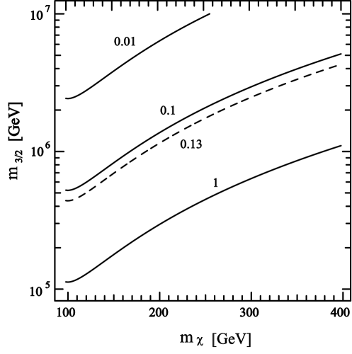
FIG. 1.: Constant contours of the density parameter $\Omega_{\chi}h^{2}$ are drawn in the $m_{\chi}$-$m_{3/2}$ plane. Three real lines represent $\Omega_{\chi}h^{2}=$0.01, 0.1, and 1, from the above. Also shown by a dashed line is the contour of $\Omega_{\chi}h^{2}=0.13$, approximately corresponding to the 95%CL upperbound of the cold dark matter abundance from the cosmological observations.

- [1] S.B. Giddings, S. Kachru and J. Polchinski, Phys. Rev. D66 (2002) 106006 [arXiv:hep-th/0105097].
- [2] G.D. Coughlan, W. Fischler, E.W. Kolb, S. Raby and G.G. Ross, Phys. Lett. B131 (1983) 59; B. de Carlos, J.A. Casas, F. Quevedo and E. Roulet, Phys. Lett. B318 (1993) 447 [arXiv:hep-ph/9308325]; T. Banks, D.B. Kaplan and A.E. Nelson, Phys. Rev. D49 (1994) 779 [arXiv:hep-ph/9308292].
- [3] T. Moroi, M. Yamaguchi and T. Yanagida, Phys. Lett. B342 (1995) 105 [arXiv:hep-ph/9409367].
- [4] L. Randall and S. Thomas, Nucl. Phys. B449 (1995) 229 [arXiv:hep-ph/9407248].
- [5] M. Kawasaki, T. Moroi and T. Yanagida, Phys. Lett. B 370 (1996) 52 [arXiv:hep-ph/9509399].
- [6] T. Moroi and L. Randall, Nucl. Phys. B 570, 455 (2000) [arXiv:hep-ph/9906527].
- [7] M. Dine, L. Randall and S. D. Thomas, Phys. Rev. Lett. 75 (1995) 398 [arXiv:hep-ph/9503303].
- [8] G. Lazarides, C. Panagiotakopoulos and Q. Shafi, Phys. Rev. Lett. 56 (1986) 432, Phys. Rev. Lett. 56 (1986) 557, Phys. Rev. Lett. 58 (1987) 1707.
- [9] D. H. Lyth and E. D. Stewart, Phys. Rev. D 53 (1996) 1784 [arXiv:hep-ph/9510204].
- [10] J. Yokoyama, arXiv:hep-ph/0601067.
- [11] S. Kachru, R. Kallosh, A. Linde and S.P. Trivedi, Phys. Rev. D68 (2003) 046005 [arXiv:hep-th/0301240].
- [12] K. Choi, A. Falkowski, H. P. Nilles, M. Olechowski and S. Pokorski, JHEP 0411 (2004) 076 [arXiv:hep-th/0411066].
- [13] K. Choi, A. Falkowski, H. P. Nilles and M. Olechowski, Nucl. Phys. B 718 (2005) 113 [arXiv:hep-th/0503216].
- [14] M. Endo, M. Yamaguchi and K. Yoshioka, Phys. Rev. D 72 (2005) 015004 [arXiv:hep-ph/0504036].
- [15] K. Choi, K. S. Jeong and K. Okumura, JHEP 0509 (2005) 039 [arXiv:hep-ph/0504037].
- [16] A. Falkowski, O. Lebedev and Y. Mambrini, JHEP 0511, 034 (2005) [arXiv:hep-ph/0507110].
- [17] N.V. Krasnikov, Phys. Lett. B193 (1987) 37; T.R. Taylor, Phys. Lett. B252 (1990) 59; J.A. Casas, Z. Lalak, C. Munoz and G.G. Ross, Nucl. Phys. B347 (1990) 243; B. de Carlos, J.A. Casas and C. Munoz, Nucl. Phys. B399 (1993) 623 [arXiv:hep-th/9204012].
- [18] W. Buchmuller, K. Hamaguchi, O. Lebedev and M. Ratz, Nucl. Phys. B699 (2004) 292 [arXiv:hep-th/0404168];
- [19] M. Hashimoto, K. I. Izawa, M. Yamaguchi and T. Yanagida, Prog. Theor. Phys. 100, 395 (1998) [arXiv:hep-ph/9804411].
- [20] K. Kohri, M. Yamaguchi and J. Yokoyama, Phys. Rev. D 70, 043522 (2004) [arXiv:hep-ph/0403043].
- [21] K. Kohri, M. Yamaguchi and J. Yokoyama, Phys. Rev. D 72, 083510 (2005) [arXiv:hep-ph/0502211].
- [22] S. Weinberg, Phys. Rev. Lett. 48 (1982) 1303.
- [23] M. Kawasaki, K. Kohri and T. Moroi, Phys. Lett. B 625, 7 (2005) [arXiv:astro-ph/0402490].
- [24] M. Kawasaki, K. Kohri and T. Moroi, Phys. Rev. D 71, 083502 (2005) [arXiv:astro-ph/0408426].
- [25] K. Kohri, T. Moroi and A. Yotsuyanagi, arXiv:hep-ph/0507245.
- [26] T. Moroi, PhD thesis “Effects of the gravitino on the inflationary universe,” arXiv:hep-ph/9503210.
- [27] T. Nagano and M. Yamaguchi, Phys. Lett. B 438, 267 (1998) [arXiv:hep-ph/9805204].
- [28] S. Mizuta and M. Yamaguchi, Phys. Lett. B 298, 120 (1993) [arXiv:hep-ph/9208251].
- [29] D.N. Spergel et al. [WMAP Collaboration], Astrophys. J. Suppl. 148 (2003) 175 [arXiv:astro-ph/0302209].
- [30] R. Kallosh and A. Linde, JHEP 0412, 004 (2004) [arXiv:hep-th/0411011].
- [31] L. Randall and R. Sundrum, Nucl. Phys. B557 (1999) 79 [arXiv:hep-th/9810155]; G.F. Giudice, M.A. Luty, H. Murayama and R. Rattazzi, JHEP 9812 (1998) 027 [arXiv:hep-ph/9810442]; J.A. Bagger, T. Moroi and E. Poppitz, JHEP 0004 (2000) 009 [arXiv:hep-th/9911029].
- [32] M. A. Luty, Phys. Rev. Lett. 89, 141801 (2002) [arXiv:hep-th/0205077].
- [33] H. S. Goh, S. P. Ng and N. Okada, JHEP 0601 (2006) 147 [arXiv:hep-ph/0511301].