Primordial Neutrinos

Abstract

The connection between cosmological observations and neutrino physics is discussed in detail. Neutrinos decouple from thermal contact in the early Universe at a temperature of order 1 MeV which coincides with the temperature where light element synthesis occurs. Observation of light element abundances therefore provides important information on such properties as neutrino energy density and chemical potential. Precision observations of the cosmic microwave background and large scale structure of galaxies can be used to probe neutrino masses with greater precision than current laboratory experiments. In this review I discuss current cosmological bounds on neutrino properties, as well as possible bounds from upcoming measurements.

1 Introduction

In the past few years a new standard model of cosmology has been established in which most of the energy density of the Universe is made up of cold dark matter and a component with negative pressure, generically referred to as dark energy. This model provides an amazingly good fit to all observational data with relatively few free parameters and has allowed for stringent constraints on the basic cosmological parameters.

The precision of the data is now at a level where observations of the cosmic microwave background (CMB), the large scale structure (LSS) of galaxies, and type Ia supernovae can be used to probe important aspects of particle physics such as neutrino properties. Conversely, cosmology is now also at a level where unknowns from the particle physics side can significantly bias estimates of cosmological parameters.

The prime example of this interplay between particle physics and cosmology is the use of cosmological data to probe neutrino physics. Particularly the possibility to constrain the neutrino mass using cosmological measurements has been studied extensively.

If only the three known neutrino flavour states, $\nu_{f}$, are considered, they must correspond to three mass eigenstates, $\nu_{i}$. The two sets are related by

$$\nu_{f}=U\nu_{i},$$ (1)

where $U$ is the $3\times 3$ neutrino mixing matrix.

The neutrino oscillation probability in the general $3\times 3$ oscillation case is quite complicated, but always depends on $\delta m^{2}$, i.e. on squared mass differences. The combination of all currently available data from neutrino oscillation experiments suggests two important mass differences in the neutrino mass hierarchy. The solar mass difference of $\Delta m_{12}^{2}\simeq 7.5-8.7\times 10^{-5}$ eV² $(2\sigma)$ and the atmospheric mass difference $|\Delta m_{23}^{2}|\simeq 1.7-2.9\times 10^{-3}$ eV² $(2\sigma)$ [1]. In the simplest case where neutrino masses are hierarchical these results suggest that $m_{1}\sim 0$, $m_{2}\sim\Delta m_{\rm solar}$, and $m_{3}\sim\Delta m_{\rm atmospheric}$. If the hierarchy is inverted one instead finds $m_{3}\sim 0$, $m_{2}\sim\Delta m_{\rm atmospheric}$, and $m_{1}\sim\Delta m_{\rm atmospheric}$. However, it is also possible that neutrino masses are degenerate, $m_{1}\sim m_{2}\sim m_{3}\gg\Delta m_{\rm atmospheric}$. Since oscillation probabilities depend only on squared mass differences, $\Delta m^{2}$, such experiments have no sensitivity to the absolute value of neutrino masses, and if the masses are degenerate oscillation experiments are not useful for determining the absolute mass scale.

Experiments which rely on kinematical effects of the neutrino mass offer the most robust probe of this overall mass scale. Tritium decay measurements by the Mainz experiment have been able to put an upper limit on the effective electron neutrino mass of $m_{\nu_{e}}=\left(\sum_{i}|U_{ei}|^{2}m_{i}^{2}\right)^{1/2}<2.3$ eV (95% conf.) [2] (note that this is an incoherent sum so that cancellation due to phases cannot occur). However, cosmology at present provides an even better limit, as will be discussed in detail in the next sections.

Very interestingly there is also a claim of direct detection of neutrinoless double beta decay in the Heidelberg-Moscow experiment [3, 4, 5]. Neutrinoless double beta decay is only possible if neutrinos are majorana particles because it requires violation of lepton number. The lifetime of the neutrinoless mode of the decay is inversely proportional to the square of the effective mass of the neutrino because it involves flipping the spin of the internal neutrino.

The claimed lifetime of ${}^{76}Ge$ measured by the experiment can be translated to a neutrino mass. However, there is a large uncertainty in this translation because the involved nuclear matrix element is quite difficult to calculate (see for instance [6]). Including the estimated matrix element uncertainty the result corresponds to an effective neutrino mass in the $0.1-0.9$ eV range for the parameter $m_{ee}=\left|\sum_{j}U^{2}_{ej}m_{\nu_{j}}\right|$ (note that, contrary to the tritium measurement, this is a coherent sum which means that it can be suppressed by phases in the mixing matrix). If this result is confirmed then it shows that neutrino masses are almost degenerate.

Another important question which can be answered by cosmological observations is how large the total neutrino energy density is. Apart from the standard model prediction of three light neutrinos, such energy density can be either in the form of additional, sterile neutrino degrees of freedom, or a non-zero neutrino chemical potential.

In this review I discuss mainly these two questions. Due to the limited space available other interesting aspects of neutrino cosmology, such as leptogenesis, have been left out. The interested reader is referred to the very thorough review [35].

The paper is divided into sections in the following way: In section 2 I review the thermal evolution of light neutrinos, particularly aspects related to the decoupling of neutrinos around a temperature of 1 MeV. I also discuss Big Bang nucleosynthesis and its relation to neutrino physics.

I section 3 I discuss the current cosmological data available, and section 4 contains a review of bounds on neutrino properties from this data. Finally, section 5 contains a discussion.

2 The thermal history of light neutrinos

2.1 Standard model

In the standard model neutrinos interact via weak interactions with charged leptons, keeping them in equilibrium with the electromagnetic plasma at high temperatures. Below $T\sim 30-40$ MeV $e^{+}$ and $e^{-}$ are the only relevant particles, greatly reducing the number of possible reactions which must be considered. In the absence of oscillations neutrino decoupling can be followed via the Boltzmann equation for the single particle distribution function [7]

$$\frac{\partial f}{\partial t}-Hp\frac{\partial f}{\partial p}=C_{\rm coll},$$ (2)

where $C_{\rm coll}$ represents all elastic and inelastic interactions. In the standard model all these interactions are $2\leftrightarrow 2$ interactions in which case the collision integral for process $i$ can be written

$$C_{\rm coll,i}(f_{1}) = \frac{1}{2E_{1}}\int\frac{d^{3}{\bf p}_{2}}{2E_{2}(2\pi)^{3}}\frac{d^{3}{\bf p}_{3}}{2E_{3}(2\pi)^{3}}\frac{d^{3}{\bf p}_{4}}{2E_{4}(2\pi)^{3}}$$ (3)

$$\,\,\times(2\pi)^{4}\delta^{4}(p_{1}+p_{2}-p_{3}+p_{4})\Lambda(f_{1},f_{2},f_{3},f_{4})S|M|^{2}_{12\to 34,i},$$

where $S|M|^{2}_{12\to 34,i}$ is the spin-summed and averaged matrix element including the symmetry factor $S=1/2$ if there are identical particles in initial or final states. The phase-space factor is $\Lambda(f_{1},f_{2},f_{3},f_{4})=f_{3}f_{4}(1-f_{1})(1-f_{2})-f_{1}f_{2}(1-f_{3})(1-f_{4})$.

The matrix elements for all relevant processes can for instance be found in Ref. [8]. If Maxwell-Boltzmann statistics is used for all particles, and neutrinos are assumed to be in complete scattering equilbrium so that they can be represented by a single temperature, then the collision integral can be integrated to yield the average annihilation rate for a neutrino

$$\Gamma=\frac{16G_{F}^{2}}{\pi^{3}}(g_{L}^{2}+g_{R}^{2})T^{5},$$ (4)

where

$$g_{L}^{2}+g_{R}^{2}=\cases{\sin^{4}\theta_{W}+(\frac{1}{2}+\sin^{2}\theta_{W})^{2}&for $\nu_{e}$\cr\sin^{4}\theta_{W}+(-\frac{1}{2}+\sin^{2}\theta_{W})^{2}&for $\nu_{\mu,\tau}$}.$$ (5)

This rate can then be compared with the Hubble expansion rate

$$H=1.66g_{*}^{1/2}\frac{T^{2}}{M_{\rm Pl}}$$ (6)

to find the decoupling temperature from the criterion $\left.H=\Gamma\right|_{T=T_{D}}$. From this one finds that $T_{D}(\nu_{e})\simeq 2.4$ MeV, $T_{D}(\nu_{\mu,\tau})\simeq 3.7$ MeV, when $g_{*}=10.75$, as is the case in the standard model.

This means that neutrinos decouple at a temperature which is significantly higher than the electron mass. When $e^{+}e^{-}$ annihilation occurs around $T\sim m_{e}/3$, the neutrino temperature is unaffected whereas the photon temperature is heated by a factor $(11/4)^{1/3}$. The relation $T_{\nu}/T_{\gamma}=(4/11)^{1/3}\simeq 0.71$ holds to a precision of roughly one percent. The main correction comes from a slight heating of neutrinos by $e^{+}e^{-}$ annihilation, as well as finite temperature QED effects on the photon propagator [9, 10, 11, 12, 13, 14, 8, 15, 16, 17, 18, 19, 20, 21, 22].

2.2 Big Bang nucleosynthesis and the number of neutrino species

Shortly after neutrino decoupling the weak interactions which keep neutrons and protons in statistical equilibrium freeze out. Again the criterion $\left.H=\Gamma\right|_{T=T_{\rm freeze}}$ can be applied to find that $T_{\rm freeze}\simeq 0.5g_{*}^{1/6}$ MeV [7].

Eventually, at a temperature of roughly 0.2 MeV deuterium starts to form, and very quickly all free neutrons are processed into ⁴He. The final helium abundance is therefore roughly given by

$$Y_{P}\simeq\left.\frac{2n_{n}/n_{p}}{1+n_{n}/n_{p}}\right|_{T\simeq 0.2\,\,{\rm MeV}}.$$ (7)

$n_{n}/n_{p}$ is determined by its value at freeze out, roughly by the condition that $n_{n}/n_{p}|_{T=T_{\rm freeze}}\sim e^{-(m_{n}-m_{p})/T_{\rm freeze}}$.

Since the freeze-out temperature is determined by $g_{*}$ this in turn means that $g_{*}$ can be inferred from a measurement of the helium abundance. However, since $Y_{P}$ is a function of both $\Omega_{b}h^{2}$ and $g_{*}$ it is necessary to use other measurements to constrain $\Omega_{b}h^{2}$ in order to find a bound on $g_{*}$. One customary method for doing this has been to use measurements of primordial deuterium to infer $\Omega_{b}h^{2}$ and from that calculate a bound on $g_{*}$. Usually such bounds are expressed in terms of the equivalent number of neutrino species, $N_{\nu}\equiv\rho/\rho_{\nu_{0}}$, instead of $g_{*}$. The exact value of the bound is quite uncertain because there are different and mutually inconsistent measurements of the primordial helium abundance (see for instance Ref. [23, 24] for a discussion of this issue). Some of the most recent analyses are [23] where a value of $1.7\leq N_{\nu}\leq 3.0$ (95% C.L.) was found, [25] which found $-1.14\leq\Delta N_{\nu}\leq 0.73$, and [26] which found that $N_{\nu}=3.14^{+0.7}_{-0.65}$ at 68% C.L. The difference in these results can be attributed to different assumptions about uncertainties in the primordial helium abundance. It should be noted that all these results are consistent with $N_{\nu}=3.04$, the standard model result. If a low helium abundance is assumed than the BBN bound severely restricts additional relativistic energy density beyond the standard model prediction. A full extra neutrino degree of freedom is excluded at high significance. However, that is not the case when a higher helium abundance is assumed, and the fact that the bound is dependent on assumptions should indicate that it is not a level of precision where it can be completely trusted.

Another interesting parameter which can be constrained by the same argument is the neutrino chemical potential, $\xi_{\nu}=\mu_{\nu}/T$ [27, 28, 29, 30]. At first sight this looks like it is completely equivalent to constraining $N_{\nu}$. However, this is not true because a chemical potential for electron neutrinos directly influences the $n-p$ conversion rate. Furthermore, it is crucial to take neutrino flavour oscillations into account when calculating bounds on the neutrino chemical potential. This point is discussed in more detail below.

2.3 Can neutrinos recouple?

Standard model neutrinos interact via exchange of $W$ and $Z$ bosons where the coupling strength at low energy $(E\ll m_{W,Z})$ is given by Fermi’s constant

$$G_{F}=\frac{\pi\alpha}{\sqrt{2}}\frac{1}{\sin^{2}\theta_{W}m_{W}^{2}}.$$ (8)

The $1/m_{W}^{2}$ comes from the vector boson propagator. However, at energies beyond $m_{W}$ the propagator will have $m_{W}$ replaced by momentum exchange $k$. Since this should be roughly equal to the thermal energy of an average particle in the medium, the effective interaction rate should go from

$$\Gamma\simeq G_{F}^{2}T^{5}\,\,\,(T\ll m_{W})$$ (9)

to

$$\Gamma\simeq\alpha T\,\,\,(T\gg m_{W}).$$ (10)

Comparing this with the Hubble parameter which in the radiation dominated regime is given by Eq. (6), one finds that

$$\frac{\Gamma}{H}\propto T^{-1}.$$ (11)

At high temperatures $\Gamma/H$ will be less than 1 and neutrinos will be out of equilibrium. The temperatures where this happens is roughly $T/m_{\rm Pl}\simeq\alpha/g_{*}^{1/2}\sim 10^{-3}$ which is far beyond the range where the standard model applies.

However, even if the above example is therefore not physically relevant it shows that neutrinos which interact via exchange of massless particles will always have an interaction rate (for $2\leftrightarrow 2$ processes) which is

$$\Gamma=\beta T,$$ (12)

where $\beta$ is a dimensionless quantity. Therefore such interactions will always drive neutrinos toward thermal equilibrium at late times instead of out of equilibrium.

One example which has received significant attention recently is the possibility that neutrinos couple to a massless scalar or pseudoscalar particle. If the interaction is sufficiently strong the neutrinos will come into equilibrium after BBN but before the present and consequently they will annihilate and disappear when $T\sim m_{\nu}$ [31, 32, 33]. In Fig. 1 we show $\Gamma/H$ for massless standard model neutrinos. As can be seen, neutrinos decouple from thermal equilibrium when $T\sim 1$ MeV. However for $T\gg m_{Z}$ the cross section drops and neutrinos are out of equilibrium at very early times. In the same figure we also show what happens if neutrinos couple to a light scalar, in which case they come into equilibrium at late times.

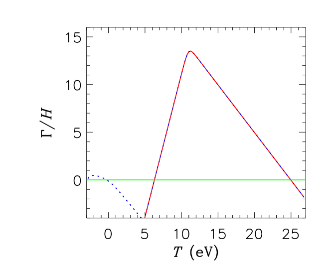
Figure 1: The interaction rate for standard a standard model neutrino is shown in red. The blue curve is for a 0.003 eV neutrino coupled to a massless scalar with dimensionless coupling $g=3\times 10^{-7}$.

2.4 The effect of oscillations

In the previous section the one-particle distribution function, $f$, was used to describe neutrino evolution. However, for neutrinos the mass eigenstates are not equivalent to the flavour eigenstates because neutrinos are mixed. Therefore the evolution of the neutrino ensemble is not in general described by the three scalar functions, $f_{i}$, but rather by the evolution of the neutrino density matrix, $\rho\equiv\psi\psi^{\dagger}$, the diagonal elements of which correspond to $f_{i}$.

For three-neutrino oscillations the formalism is quite complicated. However, the difference in $\Delta m_{12}$ and $\Delta m_{23}$, as well as the fact that $\sin 2\theta_{13}\ll 1$ means that the problem effectively reduces to a $2\times 2$ oscillation problem in the standard model. The effect of oscillations on the decoupling of neutrinos was discussed in [21, 22]. A detailed account of the physics of neutrino oscillations in the early universe is outside the scope of the present review, however an excellent and very thorough discussion of this topic can be found in Ref. [35].

Without oscillations it is possible to compensate a very large chemical potential for muon and/or tau neutrinos with a small, negative electron neutrino chemical potential [27]. However, since neutrinos are almost maximally mixed a chemical potential in one flavour can be shared with other flavours, and the end result is that during BBN all three flavours have almost equal chemical potential [36, 37, 38, 39, 40]. This in turn means that the bound on $\nu_{e}$ applies to all species. The most recent bound on the neutrino asymmetry from BBN comes from [41]

$$-0.04\leq\xi_{i}=\frac{|\eta_{i}|}{T}\leq 0.07$$ (13)

for $i=e,\mu,\tau$.

The bound assumes complete flavour equilibration during BBN, which with the measured mixing angles and mass differences is a fairly good approximation. In models where sterile neutrinos are present even more remarkable oscillation phenomena can occur. However, I do not discuss this possibility further, except for the possibility of sterile neutrino warm dark matter, and instead refer to the review [35].

2.5 Low reheating temperature and neutrinos

In most models of inflation the universe enters the normal, radiation dominated epoch at a reheating temperature, $T_{\rm RH}$, which is of order the electroweak scale or higher. However, in principle it is possible that this reheating temperature is much lower, of order MeV. This possibility has been studied many times in the literature, and a very general bound of $T_{\rm RH}\,\hbox to0.0pt{\lower 3.5pt\hbox{$\mathchar 0\relax\sim$}\hss}\raise 1.0pt\hbox{$>$}\,1$ MeV has been found [42, 43, 44, 45]

This very conservative bound comes from the fact that the light element abundances produced by big bang nucleosynthesis disagree with observations if the universe if matter dominated during BBN. However, a somewhat more stringent bound can be obtained by looking at neutrino thermalization during reheating. If a scalar particle is responsible for reheating then direct decay to neutrinos is suppressed because of the necessary helicity flip. This means that if the reheating temperature is too low neutrinos never thermalize. If this is the case then BBN predicts the wrong light element abundances. However, even if the heavy particle has a significant branching ratio into neutrinos there are problems with BBN. The reason is that neutrinos produced in decays are born with energies which are much higher than thermal. If the reheating temperature is too low then a population of high energy neutrinos will remain and also lead to conflict with observed light element abundances. Recent analyses have shown that in general the reheating temperature cannot be below a few MeV [46] (see also [47]).

3 Cosmological data

Even though BBN considerations do provide interesting bounds on neutrino physics attention has shifted towards observations of the late-time Universe. In recent years observations of physics after recombination has provided very strong constraint on many cosmological parameters and also on neutrino physics. In this section I review the current status of cosmological observations.

Large Scale Structure (LSS) –

The Sloan Digital Sky Survey (SDSS) has measured redshifts of close to 1 million galaxies, providing the so far most detailed map of the large scale structure of the Universe [48, 49]. The SDSS data has been used extensively for cosmological parameter estimation, including neutrino mass bounds. The somewhat smaller 2dFGRS (2 degree Field Galaxy Redshift Survey) [50] has also been used for the same purpose. Both surveys provide a precise measurement of the galaxy-galaxy power spectrum, $P_{g}(k)$, down to $k\sim 0.01h$/Mpc. In order to derive the matter power spectrum, $P_{m}(k)$, from this it is necessary to know the bias parameter, $b$, defined as $b^{2}(k)=P_{g}(k)/P_{m}(k)$. In general the bias parameter is scale dependent and a function of the complicated hydrodynamics of non-linear structure formation. However, if only data on scales larger than about $k\sim 0.15h$/Mpc is used the bias parameter can be taken to be a constant. In principle the bias parameter can be determined from higher-order correlations (see for instance [51, 53]), and it does provide a stringent constraint on the neutrino mass [52]. However the systematic error on the bias parameter does rely on the assumption that the non-linear aspects of structure formation are well understood, an assumption which is not necessarily justified at present. Therefore the bound on neutrino mass coming from the use of bias constraints should probably be regarded as somewhat less robust than bounds relying only on the power spectrum shape.

Cosmic Microwave Background (CMB) –

Fluctuations in the CMB were first measured by the COBE satellite in 1992 [54]. The temperature fluctuations in the CMB can be conveniently decomposed into spherical harmonics

$$\frac{\Delta T}{T}(\theta,\phi)=\sum_{lm}a_{lm}Y_{lm}(\theta,\phi).$$ (14)

From the $a_{lm}$ coefficients one can construct the angular power spectrum

$$C_{T,l}\equiv\langle|a_{lm}|^{2}\rangle,$$ (15)

where $\langle...\rangle$ denotes an ensemble average. Since only one realization of the underlying distribution is available it is in practise replaced by an angular average corresponding to averaging over $2l+1$ $m$-modes for each $l$.

The dominant scattering mechanism for photons around the apoch of recombination is Thomson scattering on free electrons. Since Thomson scattering polarizes light any anisotropy in the electron distribution leads to a net polarization anisotropy in the CMB. Like the temperature anisotropy, polarization can be written in terms of angular power spectra. Because there is no circular polarization component in the CMB there are only two independent components in the polarization tensor. The usual decomposition is in terms of curl-free $(E)$ and a curl $(B)$ component which yields four independent power spectra: $C_{T,l}$, $C_{E,l}$, $C_{B,l}$, and the $T$-$E$ cross-correlation $C_{TE,l}$. There is no cross-correlation between $B$ and $E,T$ because of different parity.

The WMAP experiment has reported data on $C_{T,l}$ and $C_{TE,l}$ as described in Refs. [55, 56, 57, 58, 59]. Foreground contamination has already been subtracted from their published data. However, it is well known that the WMAP 1-year data does exhibit some notable anomalies. First, there are several ”glitches” in the power spectrum, which are presumably due to incomplete foreground removal. Second, there is a marked suppression and alignment of the low-$w$ multipoles. There has been substantial discussion of the nature of the low-$l$ anomaly, but with no clear conclusion. Very importantly neither of the two anomalies have any influence at all on the study of neutrino properties. The reason is that neutrino physics affects only scales smaller than roughly the horizon size at recombination, and that changes to neutrino physics cannot produce sharp features in angular CMB power spectrum. Therefore, any conclusion on neutrinos is likely to hold, independent of the possible nature of the anomalies.

In addition to the WMAP data there are many independent measurements of the spectrum on smaller scales by ground based or balloon borne experiments. The most important of these at present is the Boomerang experiment [61, 62, 63] which has measured significantly smaller scales than WMAP. Furthermore, this experiment has been the first to measure $C_{E,l}$.

The baryon acoustic peak (BAO) –

In the early Universe, prior to recombination, baryons and photons undergo acoustic oscillations. These oscillations are not only detectable in the CMB, but in principle also in the LSS power spectrum. However, since baryons are only a subdominant component early structure formation is dominated by cold dark matter, and the oscillations are merely a small amplitude modulation of the power spectrum. In terms of the real-space correlation function this modulation corresponds to a well-defined peak, located at a scale of roughly 100$h^{-1}$ Mpc. This peak was first measured using the bright red galaxies of the SDSS [64]. The position of the peak provides an accurate measurement of the angular diameter distance out to redshift of roughly 0.35. This in turn provides a constraint on $\Omega_{m}$, $\Omega_{\rm DE}$, and $w$. Furthermore the constraint shows relatively little sensitivity to other parameters and seems less prone to systematics than measurements of the power spectrum amplitude.

The Lyman-$\alpha$ forest –

Measurements of the flux power spectrum of the Lyman-$\alpha$ forest has been used to measure the matter power spectrum on small scales at large redshift. This has been done using high resolution Keck or VLT spectra [65, 66]. By far the largest sample of spectra comes from the SDSS survey, even though the spectral resolution is substantially poorer than in for Keck or VLT. In Ref. [67] this data was carefully analyzed and used to constrain the linear matter power spectrum. The derived amplitude is $\Delta^{2}(k=0.009\,{\rm km\,s}^{-1},z=3)=0.452^{+0.07}_{-0.06}$ and the effective spectral index is $n_{\rm eff}=-2.321^{+0.06}_{-0.05}$. Even though the higher resolution data extend almost an order of magnitude higher in $k$ the smallest scales are likely to be completely dominated by systematics related to non-linearities so that relatively little additional information would be gained. In order to probe the mass of light neutrinos the SDSS data is therefore optimal. On the other hand the small scale data is important for testing models for warm dark matter, as will be discussed later.

The quote SDSS result has been derived using a very elaborate model for the local intergalactic medium, including full N-body simulations. It has been shown that using the Lyman-$\alpha$ data does strengthen the bound on neutrino mass significantly. However the question remains as to the level of systematic uncertainty in the result. Especially the amplitude of the matter power spectrum is quite sensitive to model assumptions. Therefore the same caution should be applied to bounds using this result as to the bound from LSS data using bias constraints, as discussed above.

Type Ia supernovae –

Measurements of distant type Ia supernovae provide a precise measurement of the luminosity distance $d_{L}$ as a function of redshift [68, 69]. This in turn provides an important constraint on $H(z)$ and therefore on $\Omega_{m}$, $\Omega_{\rm DE}$, and $w_{\rm DE}$. The most recent and precise data set comes from the SuperNova Legacy Survey (SNLS) which has published data for 71 supernovae [70]. Another data set which has been extensively used is the Riess et al. ”gold” data set [71] which consists of 157 supernovae, measured using both HST and ground based telescopes.

Other data –

Apart from the above mentioned data the measurement of the Hubble constant by the HST Hubble Key Project, $H_{0}=72\pm 8~{}{\rm km}~{}{\rm s}^{-1}~{}{\rm Mpc}^{-1}$ [72] is important for cosmological parameter analyses.

4 Neutrino Dark Matter

Neutrinos are a source of dark matter in the present day universe simply because they contribute to $\Omega_{m}$. The present temperature of massless standard model neutrinos is $T_{\nu,0}=1.95\,K=1.7\times 10^{-4}$ eV, and any neutrino with $m\gg T_{\nu,0}$ behaves like a standard non-relativistic dark matter particle.

The present contribution to the matter density of $N_{\nu}$ neutrino species with standard weak interactions is given by

$$\Omega_{\nu}h^{2}=N_{\nu}\frac{m_{\nu}}{93.8\,{\rm eV}}$$ (16)

Just from demanding that $\Omega_{\nu}\leq 1$ one finds the bound [73, 74]

$$m_{\nu}\,\hbox to0.0pt{\lower 3.5pt\hbox{$\mathchar 0\relax\sim$}\hss}\raise 1.0pt\hbox{$<$}\,\frac{46\,{\rm eV}}{N_{\nu}}$$ (17)

4.1 The Tremaine-Gunn bound

If neutrinos are the main source of dark matter, then they must also make up most of the galactic dark matter. However, neutrinos can only cluster in galaxies via energy loss due to gravitational relaxation since they do not suffer inelastic collisions. In distribution function language this corresponds to phase mixing of the distribution function [75]. By using the theorem that the phase-mixed or coarse grained distribution function must explicitly take values smaller than the maximum of the original distribution function one arrives at the condition

$$f_{\rm CG}\leq f_{\nu,{\rm max}}=\frac{1}{2}$$ (18)

Because of this upper bound it is impossible to squeeze neutrino dark matter beyond a certain limit [75]. For the Milky Way this means that the neutrino mass must be larger than roughly 25 eV if neutrinos make up the dark matter. For irregular dwarf galaxies this limit increases to 100-300 eV [76, 77], and means that standard model neutrinos cannot make up a dominant fraction of the dark matter. This bound is generally known as the Tremaine-Gunn bound.

Note that this phase space argument is a purely classical argument, it is not related to the Pauli blocking principle for fermions (although, by using the Pauli principle $f_{\nu}\leq 1$ one would arrive at a similar, but slightly weaker limit for neutrinos). In fact the Tremaine-Gunn bound works even for bosons if applied in a statistical sense [76], because even though there is no upper bound on the fine grained distribution function, only a very small number of particles reside at low momenta (unless there is a condensate). Therefore, although the exact value of the limit is model dependent, limit applies to any species that was once in thermal equilibrium. A notable counterexample is non-thermal axion dark matter which is produced directly into a condensate.

A very interesting direct example of the Tremaine-Gunn bound was studied in [78]. Here, neutrino clustering in evolving cold dark matter halos was studied using the Boltzmann equation. The problem was made tractable by assuming the backreaction, i.e. that the CDM halos are not affected by neutrinos. The results clearly show that there is a maximum in the coarse grained distribution function of $1/2$, as expected. The calculation was extended to bosons in [79], where no such upper bound was found. In fact bosons can have an average density several times higher than fermions with equal mass inside dark matter halos, an effect which in principle might be used to distinguish fermionic and bosonic hot dark matter.

4.2 Neutrino hot dark matter

A much stronger upper bound on the neutrino mass than the one in Eq. (17) can be derived by noticing that the thermal history of neutrinos is very different from that of a WIMP because the neutrino only becomes non-relativistic very late.

In an inhomogeneous universe the Boltzmann equation for a collisionless species is [80]

$$L[f]=\frac{Df}{D\tau}=\frac{\partial f}{\partial\tau}+\frac{dx^{i}}{d\tau}\frac{\partial f}{\partial x^{i}}+\frac{dq^{i}}{d\tau}\frac{\partial f}{\partial q^{i}}=0,$$ (19)

where $\tau$ is conformal time, $d\tau=dt/a$, and $q^{i}=ap^{i}$ is comoving momentum. The second term on the right-hand side has to do with the velocity of the distribution in a given spatial point and the third term is the cosmological momentum redshift.

Following Ma and Bertschinger [80] this can be rewritten as an equation for $\Psi$, the perturbed part of $f$

$$f(x^{i},q^{i},\tau)=f_{0}(q)\left[1+\Psi(x^{i},q^{i},\tau)\right]$$ (20)

In synchronous gauge that equation is

$$\frac{1}{f_{0}}[f]=\frac{\partial\Psi}{\partial\tau}+i\frac{q}{\epsilon}\mu\Psi+\frac{d\ln f_{0}}{d\ln q}\left[\dot{\eta}-\frac{\dot{h}+6\dot{\eta}}{2}\mu^{2}\right]=\frac{1}{f_{0}}C[f],$$ (21)

where $q^{j}=qn^{j}$, $\mu\equiv n^{j}\hat{k}_{j}$, and $\epsilon=(q^{2}+a^{2}m^{2})^{1/2}$. $k^{j}$ is the comoving wavevector. $h$ and $\eta$ are the metric perturbations, defined from the perturbed space-time metric in synchronous gauge [80]

$$ds^{2}=a^{2}(\tau)[-d\tau^{2}+(\delta_{ij}+h_{ij})dx^{i}dx^{j}],$$ (22)

$$h_{ij}=\int d^{3}ke^{i\vec{k}\cdot\vec{x}}\left(\hat{k}_{i}\hat{k}_{j}h(\vec{k},\tau)+(\hat{k}_{i}\hat{k}_{j}-\frac{1}{3}\delta_{ij})6\eta(\vec{k},\tau)\right).$$ (23)

Expanding this in Legendre polynomials one arrives at a set of hierarchy equations

$$\dot{\delta} = -\frac{4}{3}\theta-\frac{2}{3}\dot{h}$$

$$\dot{\theta} = k^{2}\left(\frac{\delta}{4}-\sigma\right)$$

$$2\dot{\sigma} = \frac{8}{15}\theta-\frac{3}{15}kF_{3}+\frac{4}{15}\dot{h}+\frac{8}{5}\dot{\eta}$$

$$\dot{F}_{l} = \frac{k}{2l+1}\left(lF_{l-1}-(l+1)F_{l+1}\right)$$ (24)

For subhorizon scales ($\dot{h}=\dot{\eta}=0$) this reduces to the form

$$\dot{\delta} = -\frac{4}{3}\theta$$

$$\dot{\theta} = k^{2}\left(\frac{\delta}{4}-\sigma\right)$$

$$2\dot{\sigma} = \frac{8}{15}\theta-\frac{3}{15}kF_{3}$$

$$\dot{F}_{l} = \frac{k}{2l+1}\left(lF_{l-1}-(l+1)F_{l+1}\right)$$ (25)

One should notice the similarity between this set of equations and the evolution hierarchy for spherical Bessel functions. Indeed the exact solution to the hierarchy is

$$F_{l}(k\tau)\sim j_{l}(k\tau)$$ (26)

This shows that the solution for $\delta$ is an exponentially damped oscillation. On small scales, $k>\tau$, perturbations are erased.

This in intuitively understandable in terms of free-streaming. Indeed the Bessel function solution comes from the fact that neutrinos are considered massless. In the limit of CDM the evolution hierarchy is truncated by the fact that $\theta=0$, so that the CDM perturbation equation is simply $\dot{\delta}=-\dot{h}/2$. For massless particles the free-streaming length is $\lambda=c\tau$ which is reflected in the solution to the Boltzmann hierarchy. Of course the solution only applies when neutrinos are strictly massless. Once $T\sim m$ there is a smooth transition to the CDM solution. Therefore the final solution can be separated into two parts: 1) $k>\tau(T=m)$: Neutrino perturbations are exponentially damped 2) $k<\tau(T=m)$: Neutrino perturbations follow the CDM perturbations. Calculating the free streaming wavenumber in a flat CDM cosmology leads to the simple numerical relation (applicable only for $T_{\rm eq}\gg m\gg T_{0}$) [7]

$$\lambda_{\rm FS}\sim\frac{20~{}{\rm Mpc}}{\Omega_{x}h^{2}}\left(\frac{T_{x}}{T_{\nu}}\right)^{4}\left[1+\log\left(3.9\frac{\Omega_{x}h^{2}}{\Omega_{m}h^{2}}\left(\frac{T_{\nu}}{T_{x}}\right)^{2}\right)\right]\,.$$ (27)

In Fig. 2 I have plotted transfer functions for various different neutrino masses in a flat $\Lambda$CDM universe $(\Omega_{m}+\Omega_{\nu}+\Omega_{\Lambda}=1)$. The parameters used were $\Omega_{b}=0.04$, $\Omega_{\rm CDM}=0.26-\Omega_{\nu}$, $\Omega_{\Lambda}=0.7$, $h=0.7$, and $n=1$.

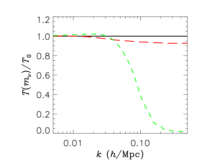
Figure 2: The transfer function $T(k,t=t_{0})$ for various different neutrino masses. The solid (black) line is for $m_{\nu}=0$, the long-dashed for $m_{\nu}=0.3$ eV, and the dashed for $m_{\nu}=1$ eV.

When measuring fluctuations it is customary to use the power spectrum, $P(k,\tau)$, defined as

$$P(k,\tau)=|\delta|^{2}(\tau).$$ (28)

The power spectrum can be decomposed into a primordial part, $P_{0}(k)$, and a transfer function $T(k,\tau)$,

$$P(k,\tau)=P_{0}(k)T(k,\tau).$$ (29)

The transfer function at a particular time is found by solving the Boltzmann equation for $\delta(\tau)$.

At scales much smaller than the free-streaming scale the present matter power spectrum is suppressed roughly by the factor [81]

$$\frac{\Delta P(k)}{P(k)}=\frac{\Delta T(k,\tau=\tau_{0})}{T(k,\tau=\tau_{0})}\simeq-8\frac{\Omega_{\nu}}{\Omega_{m}},$$ (30)

as long as $\Omega_{\nu}\ll\Omega_{m}$. The numerical factor 8 is derived from a numerical solution of the Boltzmann equation, but the general structure of the equation is simple to understand. At scales smaller than the free-streaming scale the neutrino perturbations are washed out completely, leaving only perturbations in the non-relativistic matter (CDM and baryons). Therefore the relative suppression of power is proportional to the ratio of neutrino energy density to the overall matter density. Clearly the above relation only applies when $\Omega_{\nu}\ll\Omega_{m}$, when $\Omega_{\nu}$ becomes dominant the spectrum suppression becomes exponential as in the pure hot dark matter model. This effect is shown for different neutrino masses in Fig. 2.

The effect of massive neutrinos on structure formation only applies to the scales below the free-streaming length. For neutrinos with masses of several eV the free-streaming scale is smaller than the scales which can be probed using present CMB data and therefore the power spectrum suppression can be seen only in large scale structure data. On the other hand, neutrinos of sub-eV mass behave almost like a relativistic neutrino species for CMB considerations. The main effect of a small neutrino mass on the CMB is that it leads to an enhanced early ISW effect. The reason is that the ratio of radiation to matter at recombination becomes larger because a sub-eV neutrino is still relativistic or semi-relativistic at recombination.

4.3 Neutrino mass bounds

4.3.1 Parameter estimation methodology

Because massive neutrinos affect structure formation it is possible to constrain their mass using a combination of cosmological data. The standard approach to cosmological parameter estimation is to use Bayesian statistics which provides a very simple method for incorporating prior information on parameters from other sources. Using the prior probability distribution it is then possible to calculate the posterior distribution and from that to derive confidence limits on parameters. There are standard packages such as CosmoMC [82], a likelihood calculator based on the Markov Chain Monte Carlo method [85, 86], available for this purpose.

It should be noted here that confidence limits derived using Bayesian statistics in this way are often much more stringent than implied by frequentist statistics, in which one calculates the confidence with which a given hypothesis can be excluded. The main reason for this is that observables in our Universe is a single realization of an underlying distribution. There is no possibility for producing new data to test the hypothesis and therefore the frequentist approach in many cases does not fully use the information provided by the given data. Much more detailed discussions of this point can be found in [83, 84]. In the remainder of this section we discuss only results derived using the Bayesian method.

Independent of the statistical method used results will in general depend on the number of parameters used to fit the data. Because of parameter degeneracies bounds on a given parameter will in general get weaker if more parameters are used in the fit. However, the question remains as to how many parameters should plausibly be included. If nothing is known a priori about the cosmological model the best-fit $\chi^{2}$ for $N$ parameters should in general be substantially lower for $N+1$ parameters if the additional parameter is to be included. This point has been extensively discussed in [83], and if used at face value indicates that the vanilla $\Lambda$CDM model with $n=1$ is the preferred model. This model assumes spatial flatness and uses only the following free parameters: $\Omega_{m}$, the matter density, $\Omega_{b}$, the baryon density, $H_{0}$, the Hubble parameters, $\tau$, the optical depth to reionization, and $A$, the amplitude of primordial density fluctuations. It furthermore assumes that the primordial perturbations are purely adiabatic in nature.

However, even though the best fit $\chi^{2}$ for neutrino mass is for $m_{\nu}=0$ that certainly does not mean the neutrino masses should not be included in parameter fitting. The neutrino mass is known from oscillation experiments to be non-zero and therefore must be included in parameter estimation.

Furthermore almost all studies of constraints on non-standard cosmological parameters assume the minimal $\Lambda$CDM model as the benchmark and then include the non-standard parameters specific to the given study. This approach is dangerous because there could easily be several non-standard parameters which produce a much better fit when combined. It is important to study more general models, especially since numerical techniques have now made it feasible to use many more free parameters. Below we will discuss one case where including two non-standard parameters can lead to completely changed conclusions about neutrino mass bounds.

4.3.2 Current bounds

With the WMAP data alone sensitivity to the neutrino mass is relatively limited. In a standard likelihood analysis for the 6 parameters of the minimal $\Lambda$CDM model plus neutrino mass we find an upper bound of $\sum m_{\nu}<2.1$ eV (95% C.L.). This value is consistent with that derived in other recent analyses [87, 88].

Including LSS data the bound can be improved. However, if there is no information on the normalization of the large scale structure power spectrum (the bias parameter), the improvement is relatively modest. For the same model as above the bound for WMAP+SDSS is 1.8 eV [49].

Once other data, such as type Ia supernova measurements, are included the bound can be improved significantly. A very stringent constraint comes from including information on the normalization of the matter power spectrum from measurements of the Lyman-$\alpha$ forest. In [52] a bound of $\sum m_{\nu}<0.42$ eV (95% C.L.) was derived using WMAP, SDSS, SNI-a, and Lyman-$\alpha$ data for the standard $\Lambda$CDM model with neutrino mass ([89] found an almost identical result). However, the uncertainty related to the modelling of the intergalactic medium at high redshift does make the bound model dependent.

Another very interesting bound can be derived when the measurement of the baryon acoustic oscillation (BAO) peak [64] is included [91]. Even for a very general model with 11 free parameters (adding the number of neutrino species $N_{\nu}$, a possible running of the spectral index, $\alpha_{s}$, and the dark energy equation of state, $w$) the upper bound was found to be 0.48 eV (95% C.L.) [91]. This is quite interesting because without the BAO data it was shown in [92] that there is a severe degeneracy between $\sum m_{\nu}$ and $w$. For CMB, LSS and SNI-a data the bound on $\sum m_{\nu}$ can be relaxed by as much as a factor of 3 when $w$ is allowed to vary. This degeneracy is broken by adding the BAO data because it provides a tight relation between $\Omega_{m}$ and $w$. The result is also encouraging because the systematic uncertainty in the BAO measurement is likely to be much smaller than in the Lyman-$\alpha$ forest data. Furthermore the derived best fit model is almost exactly identical to the best fit model found in [52], indicating that the Lyman-$\alpha$ and BAO data are completely consistent.

Finally, if both BAO and Lyman-$\alpha$ data is combined the bound strengthens to $\sum m_{\nu}<0.30$ eV (95% C.L.) [91], but with the same caveat with regards to the Lyman-$\alpha$ data as before.

In conclusion the current bound on the sum of neutrino masses can be in the range between 0.3 and 2 eV, depending on the data and parameters used. In general:
a) The bound on $\sum m_{\nu}$ for the minimal $\Lambda$CDM plus neutrino mass (8 parameters in total) is in the 0.5-0.6 eV range if CMB, LSS, and SNI-a data is used.
b) This bound can be relaxed by a large factor when more parameters, such as $w$ and $N_{\nu}$ are included, showing that the bound is not robust.
c) Even including several new parameters the bound can be pushed below 0.5 eV when additional data is added to the basic CMB, LSS, and SNI-a data. Either baryon acoustic oscillation or Lyman-$\alpha$ forest data can be used, with almost identical result. Especially the BAO data seem to be almost free of systematics, and consequently the bound seems to be robustly in the 0.5 eV range.
For those interested an (incomplete) list of other studies of neutrino mass bounds from cosmological data can be found in [93, 94, 95, 96, 97, 98].

In Table 1 various upper bounds on neutrino mass are summarized. The cases 1-4 are taken from [91] and show quite clearly that results are strongly dependent on data and parameters used. Also shown in this table is a selection of other recent results, all based on the standard $\Lambda$CDM plus neutrino parameter set.

In Fig. 3 we show the upper bound on the sum of neutrino masses for various cases which are presented in Table 1. Also shown in this figure is the sum of neutrino masses as a function of the mass of the lightest mass eigenstate. The red band is for the normal hierarchy and the blue is for the inverted hierarchy. All bounds were calculated assuming that the neutrino mass is shared equally between all species. As can be seen from the figure that assumption is clearly justified at present. In the same figure we also show the best fit region for the claimed detection of neutrinoless double beta decay by the Heidelberg-Moscow experiment [3, 4, 5]. There does seem to be some tension between the derived upper bound from cosmology and this result. However, at present it seems premature to exclude it based on cosmological arguments. This is particularly true because the exact value of the mass inferred from the experiment is highly uncertain because of the uncertainty in the nuclear matrix element calculation.

In this section we have discussed only active neutrino species. However, the framework applies equally well to sterile neutrinos and other light species. For instance [99] have derived stringent limits on light sterile neutrinos (see also [100]).

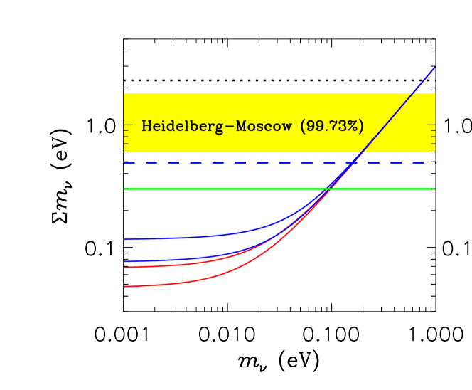
Figure 3: The 95% upper bounds on $\sum m_{\nu}$ for the different cases presented in Table 1. The horizontal axis is the mass of the lightest neutrino mass eigenstate. The set of full red lines correspond to the normal neutrino mass hierarchy and the blue to the inverted mass hierarchy. The horizontal yellow band is the claimed result from the Heidelberg-Moscow experiment. Note that the exact allowed region from this experiment is somewhat uncertain due to uncertainties in the nuclear matrix element. Figure taken from [91].

Case	$m_{\nu}$ (95% C.L.)
1: 11 parameters, CMB, LSS, SNI-a	2.3 eV
2: 11 parameters, CMB, LSS, SNI-a, BAO	0.48 eV
3: 8 parameters, CMB, LSS, SNI-a, BAO	0.44 eV
4: 8 parameters, CMB, LSS, SNI-a, BAO, Ly-$\alpha$	0.30 eV
Other recent bounds
8 parameters, WMAP only [87]	2 eV
8 parameters, WMAP, SDSS [49]	1.8 eV
8 parameters, WMAP, SDSS, SNI-a, Ly-$\alpha$ [52]	0.42 eV

Table 1: Mass bounds using different sets of data and parameters (taken from [91].

4.3.3 Neutrino interactions beyond the standard model

The mass bounds derived from cosmology depend on the assumption that neutrinos have no interactions beyond the standard model weak interactions. However, experimental constraints on non-standard neutrino interactions are in general quite weak and allows for the possibility of new, cosmologically important interactions. One example is neutrinos coupling to a light scalar or pseudoscalar, as was discussed in Section 2.3. In this case neutrinos come into thermal equilibrium with the scalar late in the evolution of the Universe. This was studied in [31] as a possible way of circumventing the cosmological bound on neutrino masses. The idea is that neutrinos coupling to a new massless degree of freedom will annihilate and disappear once $T\sim m_{\nu}$, leaving only little imprint on large scale structure. However, neutrinos which are strongly coupled will undergo acoustic oscillations prior to CMB formation instead of damping via free streaming (anisotropic stress). Since neutrino perturbations act as a source term for the baryon-photon oscillations this will increase the amplitude of CMB anisotropies on scales small than the horizon scale at recombination. This effect was studied numerically in [32, 101, 102]. Both studies find that this effect disfavours strongly coupled neutrinos, although the exact level of significance differs. The same effect was also studied analytically in [103, 104, 105]. It should be noted that [32, 102] studied the effect only in the strong coupling limit. In the intermediate regime the situation is more complicated (see [33]).

The fact that strongly interacting neutrinos are disfavoured by CMB and LSS data means that any model producing neutrino interactions strong enough to fast momentum exchange around the epoch of recombination [34]. In the case of interactions with a light pseudoscalar like the majoron this leads to a very rough bound on the diagonal coupling $g_{ii}$ of $10^{-7}$ from consideration of pair creation and annihilation processes. For the off-diagonal coupling it is roughly $g_{ij}<10^{-11}(0.05{\rm eV}/m)^{2}$ which is in fact the strongest known bound on these parameters. An exact calculation of the bound would require a solution of the Boltzmann equation for neutrinos in the intermediate coupling regime around recombination.

Another possibility which has received quite a lot of attention recently is the possibility of neutrinos coupling to a very light scalar field [106] (see also [107, 108]). In this case the coupling can produce an effective neutrino mass which is density dependent (mass varying neutrinos), and by tuning the coupling it is possible to have the combined neutrino-scalar fluid have an effective equation of state close to $w=-1$, i.e. dark energy. It was subsequently argued that the particular form of the potential in [106] leads to a small scale instability which drives $w$ to 0 [109] (see also [110]). However, this instability apparently requires two conditions to be fulfilled: a) The effective mass of the light scalar should have $m>>H$ and b) The equation of state should obey $w>-1$. Both these conditions can be violated by other potentials (see for instance [111, 112]). Mass varying neutrinos have been discussed in other contexts, for instance in [113, 114, 115, 116].

4.3.4 The number of neutrino species - joint CMB and BBN analysis

The BBN bound on the number of neutrino species presented in the previous section can be complemented by a similar bound from observations of the CMB and large scale structure. The CMB depends on $N_{\nu}$ mainly because of the early Integrated Sachs Wolfe effect which increases fluctuation power at scales slightly larger than the first acoustic peak. The large scale structure spectrum depends on $N_{\nu}$ because the scale of matter-radiation equality is changed by varying $N_{\nu}$.

Many recent papers have used CMB, LSS, and SNI-a data to calculate bounds bounds on $N_{\nu}$ [119, 118, 120, 23, 117], and some of the bounds are listed in Table 2. Recent analyses combining BBN, CMB, and large scale structure data can be found in [118, 23], and these results are also listed in Table 2.

Common for all the bounds is that $N_{\nu}=0$ is ruled out by both BBN and CMB/LSS. This has the important consequence that the cosmological neutrino background has been positively detected, not only during the BBN epoch, but also much later, during structure formation.

The most recent bound which uses the SNI-a ”gold” data set, as well as the new Boomerang CMB data finds a limit of $N_{\nu}=4.2^{+1.7}_{-1.2}$ at 95% C.L. [121]. The bound from late-time observations is now as good as that from BBN, and the two derived value are mutually consistent given the systematic uncertainties in the primordial helium abundance.

In Fig. 4 we show the currently allowed region for $\Omega_{b}h^{2}$ and $N_{\nu}$ (taken from [121]), showing the overlap between BBN constraints and the CMB+LSS+SNI-a constraint.

In principle, even if the neutrino mass is very small, it could be possible to detect the difference between additional relativistic energy density, parameterized by $N_{\nu}$, and a non-thermal distribution of the active neutrinos [122]. However, it is unlikely that the precision of observational data from planned experiments will be sufficient to measure the difference.

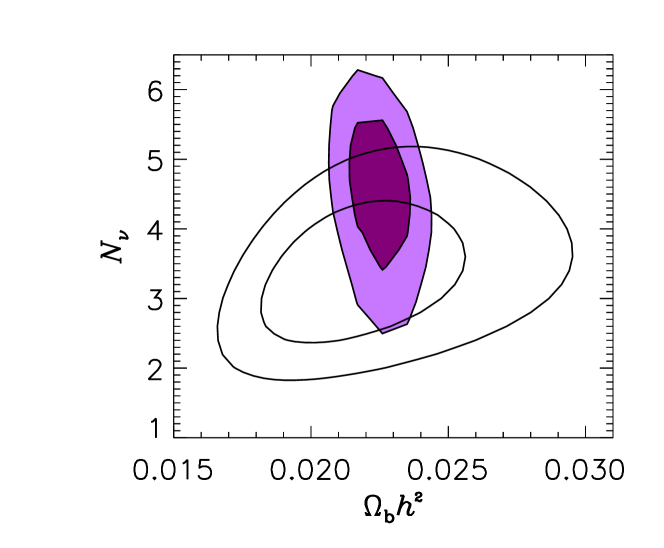
Figure 4: The 68% (dark) and 95% (light) likelihood contours for $\Omega_{b}h^{2}$ and $N_{\nu}$ for all available data. The other contours are 68% and 95% regions for BBN, assuming the ⁴He and D values given in [26]. Figure taken from [121].

Table 2: Various recent limits on the effective number of neutrino species, as well as the data used.

Ref.	Bound on $N_{\nu}$ (95% C.L.)	Data used
Crotty et al. [119]	$1.4\leq N_{\nu}\leq 6.8$	CMB, LSS
Hannestad [118]	$0.9\leq N_{\nu}\leq 7.0$	CMB, LSS
Pierpaoli [120]	$1.9\leq N_{\nu}\leq 6.62$	CMB, LSS
Barger et al. [23]	$0.9\leq N_{\nu}\leq 8.3$	CMB
Hannestad [121]	$3.0\leq N_{\nu}\leq 5.9$	CMB, LSS, SNI-a

4.3.5 Future neutrino mass measurements

The present bound on the sum of neutrino masses is still much larger than the mass difference, $|\Delta m_{23}|\sim 0.05$ eV [124, 123], measured by atmospheric neutrino observatories and K2K . This means that if the sum of neutrino masses is anywhere close to saturating the bound then neutrino masses must the almost degenerate. The question is whether in the future it will be possible to measure masses which are of the order $\Delta m_{23}$, i.e. whether it can determined if neutrino masses are hierarchical.

By combining future CMB data from the Planck satellite with a galaxy survey like the SDSS it has been estimated that neutrino masses as low as about 0.1 eV can be detected [125, pastor04] when analyzed within the minimal 8 parameter $\Lambda$CDM model. However, the degeneracy between $\sum m_{\nu}$ and $w$ found in present data is likely to persist even with much more accurate future data [92], limiting the precision with which the neutrino mass can be measured.

One very powerful probe which will become available in the future is weak gravitational lensing. With future CMB experiments like Planck [130] and the proposed Inflation Probe [131] it will be possible to measure lensing effects on the CMB itself. In this case it seems likely that a sensitivity below 0.1 eV can also be reached with CMB alone [127, 128, 129].

Another possibility is to probe weak lensing at much lower redshifts. This can be done by measuring lensing of background galaxies by large scale structure. This has the major advantage that it is possible to perform lensing tomography by binning data in different redshift bins. In [132] the projected sensitivity from combining future CMB data with a large scale weak lensing survey was studied. It was estimated that at $1\sigma$ the sensitivity could be pushed to 0.03 eV. Such lensing surveys are planned with experiments such as the Large Synaptic Survey Telescope (LSST) which is planned to start in 2012 [135]. At present the systematic uncertainties related to such surveys is to some extent unknown. One source of error is related to the uncertainty in measurements of galaxy shapes and another is related to the fact the redshift of galaxies must be estimated photometrically since spectroscopy is not feasible for the large number of galaxies needed. Estimates in general show that it will be possible to control the errors at the required level [133, 134].

Another promising tool which could further increase sensitivity is to use future cluster surveys [136]. Such a survey could also bring the sensitivity to 0.03 eV.

As noted in Ref. [pastor04] the exact value of the sensitivity at this level depends both on whether the hierarchy is normal or inverted, and the exact value of the mass splittings. At this level, neutrino masses cannot be regarded as degenerate and the normal and inverted hierarchy models must be tested separately.

4.4 Neutrino warm dark matter

While CDM is defined as consisting of non-interacting particles which have essentially no free-streaming on any astronomically relevant scale, and HDM is defined by consisting of particles which become non-relativistic around matter radiation equality or later, warm dark matter is an intermediate. One of the simplest production mechanisms for warm dark matter is active-sterile neutrino oscillations in the early universe [138, 139, 140, 141, 142].

One possible benefit of warm dark matter is that it does have some free-streaming so that structure formation is suppressed on very small scales. This has been proposed as an explanation for the apparent discrepancy between observations of galaxies and numerical CDM structure formation simulations. In general simulations produce galaxy halos which have very steep inner density profiles $\rho\propto r^{\alpha}$, where $\alpha\sim 1-1.5$, and numerous subhalos [143, 144]. Neither of these characteristics are seen in observations and the explanation for this discrepancy remains an open question. If dark matter is warm instead of cold, with a free-streaming scale comparable to the size of a typical galaxy subhalo then the amount of substructure is suppressed, and possibly the central density profile is also flattened [145, 146, 147, 148, 149, 150, 151] . In both cases the mass of the dark matter particle should be around 0.5 – 1 keV [153, 154, 155], assuming that it is thermally produced in the early universe.

On the other hand, from measurements of the Lyman-$\alpha$ forest flux power spectrum it has been possible to reconstruct the matter power spectrum on relatively small scales at high redshift. This spectrum does not show any evidence for suppression at sub-galaxy scales and has been used to put a lower bound on the mass of warm dark matter particles of roughly 500 eV [156]. An even more severe problem lies in the fact that star formation occurs relatively late in warm dark matter models because small scale structure is suppressed. This may be in conflict with the low-$l$ CMB temperature-polarization cross correlation measurement by WMAP which indicates very early reionization and therefore also early star formation. One recent investigation of this found warm dark matter to be inconsistent with WMAP for masses as high as 10 keV [145].

Very interestingly a keV sterile neutrino will decay radiatively and produce x-ray photons which can reionize the Universe at high redshift. The decay lifetime is given purely in terms of the mass and mixing angle with active species

$$\tau=5\times 10^{28}\left(\frac{7\,{\rm keV}}{m}\right)^{5}\left(\frac{0.8\times 10^{-9}}{\sin^{2}\theta}\right)\,{\rm s}.$$ (31)

Since the total contribution to the energy density is also given purely in terms of these parameters (assuming a zero lepton assymetry) it is possible to calculate the total x-ray photon intensity as a function of redshift.

Such decays have been proposed as a possible explanation for the very high optical depth indicated by the WMAP polarization measurement which seems to require partial reionization already at $z\sim 15-20$ [157, 158, 159, 160]. However, in this case the mass must be several keV in order to have a short enough lifetime (since $\tau\propto m^{-5}$). Therefore there does not seem to be a common mass which can address both the structure formation problems and the reionization problems.

The case for warm dark matter seems quite marginal, although at present it is not definitively ruled out by any observations.

5 Discussion

In the present paper I have discussed how cosmological observations can be used for probing fundamental properties of neutrinos which are not easily accessible in lab experiments. Particularly the measurement of absolute neutrino masses from CMB and large scale structure data has received significant attention over the past few years. From cosmological observations it has been possible to derive an upper bound on the sum of neutrino masses which seems to be robustly in the 0.5 eV range. This is substantially better than the present bound from tritium decay measurements which is $m_{\nu_{e}}<2.3$ eV (95% C.L.), leading to $\sum m_{\nu}\,\hbox to0.0pt{\lower 3.5pt\hbox{$\mathchar 0\relax\sim$}\hss}\raise 1.0pt\hbox{$<$}\,7$ eV.

In the future this type of measurement will be improved by more than an order of magnitude by the KATRIN experiment [162, 161] which has a projected sensitivity of 0.2 eV on the effective electron neutrino mass.

Another cornerstone of neutrino cosmology is the measurement of the total energy density in non-electromagnetically interacting particles. For many years Big Bang nucleosynthesis was the only probe of relativistic energy density, but with the advent of precision CMB and LSS data it has been possible to complement the BBN measurement. At present the cosmic neutrino background is seen in both BBN, CMB and LSS data at high significance, with $N_{\nu}=0$ being excluded at more than $5\sigma$.

Finally, cosmology can also be used to probe the possibility of neutrino warm dark matter, which could be produced by active-sterile neutrino oscillations.

In the coming years the steady stream of new observational data will continue, and the cosmological bounds on neutrino will improve accordingly. For instance, it has been estimated that with data from the upcoming Planck satellite it could be possible to measure neutrino masses as low as 0.05 eV which would allow for a determination of the neutrino mass even in the normal hierarchy.

References

- [1] M. Maltoni, T. Schwetz, M. A. Tortola and J. W. F. Valle, New J. Phys. 6, 122 (2004) [arXiv:hep-ph/0405172].
- [2] C. Kraus et al. European Physical Journal C (2003), proceedings of the EPS 2003 - High Energy Physics (HEP) conference.
- [3] H. V. Klapdor-Kleingrothaus, A. Dietz, H. L. Harney and I. V. Krivosheina, Mod. Phys. Lett. A 16, 2409 (2001) [arXiv:hep-ph/0201231].
- [4] H. V. Klapdor-Kleingrothaus, I. V. Krivosheina, A. Dietz and O. Chkvorets, Phys. Lett. B 586, 198 (2004) [arXiv:hep-ph/0404088].
- [5] H. Volker Klapdor-Kleingrothaus, arXiv:hep-ph/0512263.
- [6] A. Faessler, Nucl. Phys. Proc. Suppl. 145, 213 (2005).
- [7] E. W. Kolb and M. S. Turner, “The Early Universe,”, Addison-Wesley (1990).
- [8] S. Hannestad and J. Madsen, Phys. Rev. D 52, 1764 (1995) [arXiv:astro-ph/9506015].
- [9] D. A. Dicus, E. W. Kolb, A. M. Gleeson, E. C. Sudarshan, V. L. Teplitz and M. S. Turner, Phys. Rev. D 26, 2694 (1982).
- [10] N. C. Rana and B. Mitra, Phys. Rev. D 44, 393 (1991).
- [11] M. A. Herrera and S. Hacyan, Astrophys. J. 336, 539 (1989).
- [12] A. D. Dolgov and M. Fukugita, Phys. Rev. D 46, 5378 (1992).
- [13] S. Dodelson and M. S. Turner, Phys. Rev. D 46, 3372 (1992).
- [14] B. D. Fields, S. Dodelson and M. S. Turner, Phys. Rev. D 47, 4309 (1993) [arXiv:astro-ph/9210007].
- [15] A. D. Dolgov, S. H. Hansen and D. V. Semikoz, Nucl. Phys. B 503, 426 (1997) [arXiv:hep-ph/9703315].
- [16] A. D. Dolgov, S. H. Hansen and D. V. Semikoz, Nucl. Phys. B 543, 269 (1999) [arXiv:hep-ph/9805467].
- [17] N. Y. Gnedin and O. Y. Gnedin, Astrophys. J. 509, 11 (1998).
- [18] S. Esposito, G. Miele, S. Pastor, M. Peloso and O. Pisanti, Nucl. Phys. B 590, 539 (2000) [arXiv:astro-ph/0005573].
- [19] G. Steigman, arXiv:astro-ph/0108148.
- [20] G. Mangano, G. Miele, S. Pastor and M. Peloso, arXiv:astro-ph/0111408.
- [21] S. Hannestad, Physical Review D 65, 083006 (2002).
- [22] G. Mangano, G. Miele, S. Pastor, T. Pinto, O. Pisanti and P. D. Serpico, Nucl. Phys. B 729, 221 (2005) [arXiv:hep-ph/0506164].
- [23] V. Barger, J. P. Kneller, H. S. Lee, D. Marfatia and G. Steigman, Phys. Lett. B 566, 8 (2003) [arXiv:hep-ph/0305075].
- [24] G. Steigman, Int. J. Mod. Phys. E 15, 1 (2006) [arXiv:astro-ph/0511534].
- [25] P. D. Serpico, S. Esposito, F. Iocco, G. Mangano, G. Miele and O. Pisanti, JCAP 0412 (2004) 010 [arXiv:astro-ph/0408076].
- [26] R. H. Cyburt, B. D. Fields, K. A. Olive and E. Skillman, Astropart. Phys. 23, 313 (2005) [arXiv:astro-ph/0408033].
- [27] H. S. Kang and G. Steigman, Nucl. Phys. B 372, 494 (1992).
- [28] K. Kohri, M. Kawasaki and K. Sato, Astrophys. J. 490, 72 (1997) [arXiv:astro-ph/9612237].
- [29] M. Orito, T. Kajino, G. J. Mathews and Y. Wang, Phys. Rev. D 65, 123504 (2002) [arXiv:astro-ph/0203352].
- [30] K. Ichikawa and M. Kawasaki, Phys. Rev. D 67, 063510 (2003) [arXiv:astro-ph/0210600].
- [31] J. F. Beacom, N. F. Bell and S. Dodelson, Phys. Rev. Lett. 93, 121302 (2004) [arXiv:astro-ph/0404585].
- [32] S. Hannestad, JCAP 0502, 011 (2005) [arXiv:astro-ph/0411475].
- [33] R. F. Sawyer, arXiv:astro-ph/0601525.
- [34] S. Hannestad and G. Raffelt, Phys. Rev. D 72, 103514 (2005) [arXiv:hep-ph/0509278].
- [35] A. D. Dolgov, Phys. Rept. 370, 333 (2002) [arXiv:hep-ph/0202122].
- [36] C. Lunardini and A. Y. Smirnov, Phys. Rev. D 64, 073006 (2001) [arXiv:hep-ph/0012056].
- [37] S. Pastor, G. G. Raffelt and D. V. Semikoz, Phys. Rev. D 65, 053011 (2002) [arXiv:hep-ph/0109035].
- [38] A. D. Dolgov, S. H. Hansen, S. Pastor, S. T. Petcov, G. G. Raffelt and D. V. Semikoz, Nucl. Phys. B 632, 363 (2002) [arXiv:hep-ph/0201287].
- [39] K. N. Abazajian, J. F. Beacom and N. F. Bell, Phys. Rev. D 66, 013008 (2002) [arXiv:astro-ph/0203442].
- [40] Y. Y. Wong, Phys. Rev. D 66, 025015 (2002) [arXiv:hep-ph/0203180].
- [41] P. D. Serpico and G. G. Raffelt, Phys. Rev. D 71, 127301 (2005) [arXiv:astro-ph/0506162].
- [42] M. Kawasaki, K. Kohri and N. Sugiyama, Phys. Rev. Lett. 82, 4168 (1999) [arXiv:astro-ph/9811437].
- [43] M. Kawasaki, K. Kohri and N. Sugiyama, Phys. Rev. D 62, 023506 (2000) [arXiv:astro-ph/0002127].
- [44] G. F. Giudice, E. W. Kolb and A. Riotto, Phys. Rev. D 64, 023508 (2001) [arXiv:hep-ph/0005123].
- [45] G. F. Giudice, E. W. Kolb, A. Riotto, D. V. Semikoz and I. I. Tkachev, Phys. Rev. D 64, 043512 (2001) [arXiv:hep-ph/0012317].
- [46] S. Hannestad, Phys. Rev. D 70, 043506 (2004) [arXiv:astro-ph/0403291].
- [47] K. Ichikawa, M. Kawasaki and F. Takahashi, Phys. Rev. D 72, 043522 (2005) [arXiv:astro-ph/0505395].
- [48] M. Tegmark et al. [SDSS Collaboration], Astrophys. J. 606, 702 (2004) [arXiv:astro-ph/0310725].
- [49] M. Tegmark et al. [SDSS Collaboration], Phys. Rev. D 69, 103501 (2004) [arXiv:astro-ph/0310723].
- [50] J. A. Peacock et al., Nature 410 (2001) 169 [astro-ph/0103143].
- [51] L. Verde et al., Mon. Not. Roy. Astron. Soc. 335, 432 (2002) [arXiv:astro-ph/0112161].
- [52] U. Seljak et al., Phys. Rev. D 71, 103515 (2005) [arXiv:astro-ph/0407372].
- [53] U. Seljak et al., Phys. Rev. D 71, 043511 (2005) [arXiv:astro-ph/0406594].
- [54] G. F. Smoot et al., Astrophys. J. 396, L1 (1992).
- [55] D. N. Spergel et al., Astrophys. J. Suppl. 148 (2003) 175 [astro-ph/0302209].
- [56] C. L. Bennett et al., Preliminary maps and basic results,” Astrophys. J. Suppl. 148 (2003) 1 [astro-ph/0302207].
- [57] A. Kogut et al., Astrophys. J. Suppl. 148 (2003) 161 [astro-ph/0302213].
- [58] G. Hinshaw et al., Astrophys. J. Suppl. 148 (2003) 135 [astro-ph/0302217].
- [59] L. Verde et al., Astrophys. J. Suppl. 148 (2003) 195 [astro-ph/0302218].
- [60] H. V. Peiris et al., Astrophys. J. Suppl. 148 (2003) 213 [astro-ph/0302225].
- [61] W. C. Jones et al., arXiv:astro-ph/0507494.
- [62] F. Piacentini et al., arXiv:astro-ph/0507507.
- [63] T. E. Montroy et al., arXiv:astro-ph/0507514.
- [64] D. J. Eisenstein et al., Astrophys. J. 633, 560 (2005) [arXiv:astro-ph/0501171].
- [65] R. A. C. Croft et al., Astrophys. J. 581, 20 (2002) [arXiv:astro-ph/0012324].
- [66] T. S. Kim, M. Viel, M. G. Haehnelt, R. F. Carswell and S. Cristiani, Mon. Not. Roy. Astron. Soc. 347, 355 (2004) [arXiv:astro-ph/0308103].
- [67] P. McDonald et al., Astrophys. J. 635, 761 (2005) [arXiv:astro-ph/0407377].
- [68] A. G. Riess et al. [Supernova Search Team Collaboration], Astron. J. 116 (1998) 1009 [arXiv:astro-ph/9805201].
- [69] S. Perlmutter et al. [Supernova Cosmology Project Collaboration], Astrophys. J. 517 (1999) 565 [arXiv:astro-ph/9812133].
- [70] P. Astier et al., arXiv:astro-ph/0510447.
- [71] A. G. Riess et al. [Supernova Search Team Collaboration], Astrophys. J. 607 (2004) 665 [astro-ph/0402512].
- [72] W. L. Freedman et al., Astrophys. J. 553 (2001) 47 [astro-ph/0012376].
- [73] S. S. Gershtein and Y. B. Zeldovich, JETP Lett. 4, 120 (1966) [Pisma Zh. Eksp. Teor. Fiz. 4, 174 (1966)].
- [74] R. Cowsik and J. McClelland, Phys. Rev. Lett. 29, 669 (1972).
- [75] S. Tremaine and J. E. Gunn, Phys. Rev. Lett. 42, 407 (1979).
- [76] J. Madsen, Phys. Rev. D 44, 999 (1991).
- [77] P. Salucci and A. Sinibaldi, Astron. Astrophys. 323, 1 (1997).
- [78] A. Ringwald and Y. Y. Y. Wong, JCAP 0412, 005 (2004) [arXiv:hep-ph/0408241].
- [79] S. Hannestad, A. Ringwald, H. Tu and Y. Y. Y. Wong, JCAP 0509, 014 (2005) [arXiv:astro-ph/0507544].
- [80] C. P. Ma and E. Bertschinger, Astrophys. J. 455, 7 (1995) [arXiv:astro-ph/9506072].
- [81] W. Hu, D. J. Eisenstein and M. Tegmark, Phys. Rev. Lett. 80 (1998) 5255 [astro-ph/9712057].
- [82] http://cosmologist.info/cosmomc/
- [83] A. R. Liddle, Mon. Not. Roy. Astron. Soc. 351, L49 (2004) [arXiv:astro-ph/0401198].
- [84] R. Trotta, arXiv:astro-ph/0504022.
- [85] N. Christensen, R. Meyer, L. Knox and B. Luey, Class. Quant. Grav. 18, 2677 (2001) [arXiv:astro-ph/0103134].
- [86] A. Lewis and S. Bridle, Phys. Rev. D 66, 103511 (2002) [arXiv:astro-ph/0205436].
- [87] K. Ichikawa, M. Fukugita and M. Kawasaki, Phys. Rev. D 71, 043001 (2005) [arXiv:astro-ph/0409768].
- [88] J. Lesgourgues, private communication.
- [89] G. L. Fogli, E. Lisi, A. Marrone, A. Melchiorri, A. Palazzo, P. Serra and J. Silk, Phys. Rev. D 70, 113003 (2004) [arXiv:hep-ph/0408045].
- [90] O. Elgaroy and O. Lahav, New J. Phys. 7, 61 (2005) [arXiv:hep-ph/0412075].
- [91] A. Goobar, S. Hannestad, E. Mörtsell, H. Tu, astro-ph/0602155
- [92] S. Hannestad, Phys. Rev. Lett. 95, 221301 (2005) [arXiv:astro-ph/0505551].
- [93] O. Elgaroy and O. Lahav, JCAP 0304 (2003) 004 [astro-ph/0303089].
- [94] S. Hannestad and G. Raffelt, JCAP 0404, 008 (2004) [arXiv:hep-ph/0312154].
- [95] P. Crotty, J. Lesgourgues and S. Pastor, Phys. Rev. D 69, 123007 (2004) [arXiv:hep-ph/0402049].
- [96] S. Hannestad, Phys. Rev. D 66 (2002) 125011 [astro-ph/0205223].
- [97] S. W. Allen, R. W. Schmidt and S. L. Bridle, Mon. Not. Roy. Astron. Soc. 346, 593 (2003) [arXiv:astro-ph/0306386].
- [98] V. Barger, D. Marfatia and A. Tregre, Phys. Lett. B 595, 55 (2004) [arXiv:hep-ph/0312065].
- [99] S. Dodelson, A. Melchiorri and A. Slosar, arXiv:astro-ph/0511500.
- [100] S. Goswami and W. Rodejohann, arXiv:hep-ph/0512234.
- [101] R. Trotta and A. Melchiorri, “Indication for primordial anisotropies in the neutrino background from WMAP and SDSS,” Phys. Rev. Lett. 95, 011305 (2005) [astro-ph/0412066].
- [102] N. F. Bell, E. Pierpaoli and K. Sigurdson, arXiv:astro-ph/0511410.
- [103] S. Bashinsky and U. Seljak, “Signatures of relativistic neutrinos in CMB anisotropy and matter clustering,” Phys. Rev. D 69, 083002 (2004) [astro-ph/0310198].
- [104] Z. Chacko, L. J. Hall, T. Okui and S. J. Oliver, “CMB signals of neutrino mass generation,” Phys. Rev. D 70, 085008 (2004) [hep-ph/0312267].
- [105] T. Okui, “Searching for composite neutrinos in the cosmic microwave background,” JHEP 0509, 017 (2005) [hep-ph/0405083].
- [106] R. Fardon, A. E. Nelson and N. Weiner, JCAP 0410, 005 (2004) [arXiv:astro-ph/0309800].
- [107] R. D. Peccei, Phys. Rev. D 71, 023527 (2005) [arXiv:hep-ph/0411137].
- [108] P. Q. Hung and H. Pas, Mod. Phys. Lett. A 20, 1209 (2005) [arXiv:astro-ph/0311131].
- [109] N. Afshordi, M. Zaldarriaga and K. Kohri, Phys. Rev. D 72, 065024 (2005) [arXiv:astro-ph/0506663].
- [110] R. Takahashi and M. Tanimoto, arXiv:astro-ph/0601119.
- [111] A. W. Brookfield, C. van de Bruck, D. F. Mota and D. Tocchini-Valentini, arXiv:astro-ph/0512367.
- [112] M. Kaplinghat and A. Rajaraman, arXiv:astro-ph/0601517.
- [113] V. Barger, P. Huber and D. Marfatia, Phys. Rev. Lett. 95, 211802 (2005) [arXiv:hep-ph/0502196].
- [114] M. Cirelli, M. C. Gonzalez-Garcia and C. Pena-Garay, Nucl. Phys. B 719, 219 (2005) [arXiv:hep-ph/0503028].
- [115] M. C. Gonzalez-Garcia, P. C. de Holanda and R. Zukanovich Funchal, arXiv:hep-ph/0511093.
- [116] T. Schwetz and W. Winter, arXiv:hep-ph/0511177.
- [117] A. Cuoco, F. Iocco, G. Mangano, G. Miele, O. Pisanti and P. D. Serpico, Int. J. Mod. Phys. A 19, 4431 (2004) [arXiv:astro-ph/0307213].
- [118] S. Hannestad, JCAP 0305 (2003) 004 [astro-ph/0303076].
- [119] P. Crotty, J. Lesgourgues and S. Pastor, Phys. Rev. D 67, 123005 (2003) [arXiv:astro-ph/0302337].
- [120] E. Pierpaoli, Mon. Not. Roy. Astron. Soc. 342, L63 (2003) [arXiv:astro-ph/0302465].
- [121] S. Hannestad, arXiv:astro-ph/0510582.
- [122] A. Cuoco, J. Lesgourgues, G. Mangano and S. Pastor, Phys. Rev. D 71, 123501 (2005) [arXiv:astro-ph/0502465].
- [123] M. Maltoni, T. Schwetz, M. A. Tortola and J. W. F. Valle, Phys. Rev. D 68, 113010 (2003) [arXiv:hep-ph/0309130].
- [124] G. L. Fogli, E. Lisi, A. Marrone and D. Montanino, Phys. Rev. D 67, 093006 (2003) [arXiv:hep-ph/0303064].
- [125] S. Hannestad, Phys. Rev. D 67 (2003) 085017 [astro-ph/0211106].
- [126] J. Lesgourgues, S. Pastor and L. Perotto, Phys. Rev. D 70, 045016 (2004) [arXiv:hep-ph/0403296].
- [127] K. N. Abazajian and S. Dodelson, Phys. Rev. Lett. 91 (2003) 041301 [astro-ph/0212216].
- [128] M. Kaplinghat, L. Knox and Y. S. Song, Phys. Rev. Lett. 91, 241301 (2003) [arXiv:astro-ph/0303344].
- [129] J. Lesgourgues, L. Perotto, S. Pastor and M. Piat, arXiv:astro-ph/0511735.
- [130] http://sci.esa.int/science-e/www/area/index.cfm?fareaid=17
- [131] http://cfa-www.harvard.edu/cip/
- [132] Y. S. Song and L. Knox, arXiv:astro-ph/0312175.
- [133] D. Huterer, M. Takada, G. Bernstein and B. Jain, Mon. Not. Roy. Astron. Soc. 366, 101 (2006) [arXiv:astro-ph/0506030].
- [134] Z. M. Ma, W. Hu and D. Huterer, arXiv:astro-ph/0506614.
- [135] http://www.lsst.org
- [136] S. Wang, Z. Haiman, W. Hu, J. Khoury and M. May, Phys. Rev. Lett. 95 (2005) 011302 [arXiv:astro-ph/0505390].
- [137] V. K. Narayanan, D. N. Spergel, R. Dave and C. P. Ma, arXiv:astro-ph/0005095.
- [138] S. H. Hansen, J. Lesgourgues, S. Pastor and J. Silk, Mon. Not. Roy. Astron. Soc. 333, 544 (2002) [arXiv:astro-ph/0106108].
- [139] K. Abazajian, G. M. Fuller and W. H. Tucker, Astrophys. J. 562, 593 (2001) [arXiv:astro-ph/0106002].
- [140] K. Abazajian, G. M. Fuller and M. Patel, Phys. Rev. D 64, 023501 (2001) [arXiv:astro-ph/0101524].
- [141] X. d. Shi and G. M. Fuller, Phys. Rev. Lett. 82, 2832 (1999) [arXiv:astro-ph/9810076].
- [142] S. Dodelson and L. M. Widrow, Phys. Rev. Lett. 72, 17 (1994) [arXiv:hep-ph/9303287].
- [143] S. Kazantzidis, L. Mayer, C. Mastropietro, J. Diemand, J. Stadel and B. Moore, arXiv:astro-ph/0312194.
- [144] S. Ghigna, B. Moore, F. Governato, G. Lake, T. Quinn and J. Stadel, Astrophys. J. 544, 616 (2000) [arXiv:astro-ph/9910166].
- [145] N. Yoshida, A. Sokasian, L. Hernquist and V. Springel, Astrophys. J. 591, L1 (2003) [arXiv:astro-ph/0303622].
- [146] Z. Haiman, R. Barkana and J. P. Ostriker, arXiv:astro-ph/0103050.
- [147] V. Avila-Reese, P. Colin, O. Valenzuela, E. D’Onghia and C. Firmani, arXiv:astro-ph/0010525.
- [148] P. Bode, J. P. Ostriker and N. Turok, Astrophys. J. 556, 93 (2001) [arXiv:astro-ph/0010389].
- [149] P. Colin, V. Avila-Reese and O. Valenzuela, Astrophys. J. 542, 622 (2000) [arXiv:astro-ph/0004115].
- [150] S. Hannestad and R. J. Scherrer, Phys. Rev. D 62, 043522 (2000) [arXiv:astro-ph/0003046].
- [151] J. Sommer-Larsen and A. Dolgov, arXiv:astro-ph/9912166.
- [152] S. Colombi, S. Dodelson and L. M. Widrow, Astrophys. J. 458, 1 (1996) [arXiv:astro-ph/9505029].
- [153] C. J. Hogan and J. J. Dalcanton, Phys. Rev. D 62, 063511 (2000) [arXiv:astro-ph/0002330].
- [154] J. J. Dalcanton and C. J. Hogan, Astrophys. J. 561, 35 (2001) [arXiv:astro-ph/0004381].
- [155] T. Goerdt, B. Moore, J. I. Read, J. Stadel and M. Zemp, arXiv:astro-ph/0601404.
- [156] M. Viel, J. Lesgourgues, M. G. Haehnelt, S. Matarrese and A. Riotto, Phys. Rev. D 71 (2005) 063534 [arXiv:astro-ph/0501562].
- [157] S. H. Hansen and Z. Haiman, Astrophys. J. 600, 26 (2004) [arXiv:astro-ph/0305126].
- [158] S. Kasuya and M. Kawasaki, Phys. Rev. D 70, 103519 (2004) [arXiv:astro-ph/0409419].
- [159] M. Mapelli and A. Ferrara, Mon. Not. Roy. Astron. Soc. 364, 2 (2005) [arXiv:astro-ph/0508413].
- [160] P. L. Biermann and A. Kusenko, arXiv:astro-ph/0601004.
- [161] G. Drexlin [KATRIN Collaboration], Nucl. Phys. Proc. Suppl. 145, 263 (2005).
- [162] http://www-ik.fzk.de/katrin/index.html
- [163] U. Seljak and M. Zaldarriaga, Astrophys. J. 469 (1996) 437 [astro-ph/9603033]. See also the CMBFAST website at http://www.cmbfast.org