The 1-loop computation of the processes $\tilde{\chi}^{0}_{i}\tilde{\chi}^{0}_{j}\to\gamma Z$ has been performed at an arbitrary c.m. energy for any pair of MSSM neutralinos. As an application suitable for Dark Matter (DM) searches, the neutralino-neutralino annihilation is studied at the limiting case of vanishing relative velocity, describing the present DM distribution in the galactic halo; and at a relative velocity of about 0.5, determining the neutralino relic density contributions. The most useful situation is obviously for $i=j=1$, but the case of non-identical neutralinos may also be useful in some corners of the parameter space. Our results are contained in the FORTRAN code PLATONdmgZ, applying to any set of real MSSM parameters. Numerical results are also presented for a sample of 6 MSSM models, describing the various possible neutralino properties. A comparison with other existing works is also made.

PACS numbers: 12.15.-y, 14.80.Ly, 95.35+d

1 Introduction

The nature of Cold Dark Matter (DM), constituting almost 23% of the energy of the Universe, is one of the most exciting subjects of physics today [1, 2]. Within the minimal R-parity conserving Supersymmetric (SUSY) framework, a most obvious candidate for such matter is of course the lightest neutralino $\tilde{\chi}^{0}_{1}$ [1]. A striking signature for such DM would then be the detection of $\gamma$-rays obtained through the annihilation of two neutralinos [3].

The spectrum of most of these $\gamma$-rays should be continuous [3]. But once the necessary sensitivity is reached, sharp $\gamma$-rays could also be observed, induced by neutralino-neutralino annihilation at rest, to $\gamma\gamma$, $\gamma Z$ or a photon together with a neutral Higgs particle. Observing such $\gamma$-rays, with the predicted ratio of intensities, would be a really great discovery.

For identical annihilating neutralinos in the vanishing relative velocity limit, the processes $\tilde{\chi}^{0}_{1}\tilde{\chi}^{0}_{1}\to\gamma\gamma$ and $\tilde{\chi}^{0}_{1}\tilde{\chi}^{0}_{1}\to\gamma Z$ have already been studied in [4] and [5] respectively.

Subsequently, $\tilde{\chi}^{0}_{i}\tilde{\chi}^{0}_{j}\to\gamma\gamma$ has also been studied in [6], at any relative velocity and for any neutralino pair. This study is based on analytically expressing the amplitudes, in terms of Passarino-Veltman (PV) functions [7]. Such non-vanishing relative velocity results may be useful in estimating the neutralino contribution to the DM density [3]. In some, admittedly extreme corners of the parameter space, where the two lightest neutralinos may be exactly degenerate, the $(i\neq j)$-case may also be useful.

The same analytic amplitudes were then also used to study the reverse process $\gamma\gamma\to\tilde{\chi}^{0}_{i}\tilde{\chi}^{0}_{j}$ in a $\gamma\gamma$ Linear Collider ($LC_{\gamma\gamma}$) [8]; while the related amplitudes for $gg\to\tilde{\chi}^{0}_{i}\tilde{\chi}^{0}_{j}$ and $gg\to\tilde{\chi}^{0}_{i}\tilde{g}$, were used to determine the corresponding production of a pair of neutralinos [9], or a single neutralino [10], at the CERN LHC.

FORTRAN codes supplying all 1-loop contributions to these processes, for any set of real MSSM parameters at the electroweak scale, and any neutralino pair, may be obtained from [11]. These should be useful for checking the consistency of the neutralino DM identification, using collider experiments. The importance of such consistency checks can hardly be overemphasized.

The annihilation process $\tilde{\chi}^{0}_{1}\tilde{\chi}^{0}_{1}\to\gamma\gamma$, for the lightest neutralino, at any relative velocity, has also been studied recently by [12]. In this reference, an automatic numerical method is presented, which directly calculates the needed 1-loop amplitudes, starting from the Feynman diagrams. As pointed out by [12], their results for $\gamma\gamma$-annihilation, perfectly agree with those of [4] and [6].

However, [12] also gives results for $\tilde{\chi}^{0}_{1}\tilde{\chi}^{0}_{1}\to\gamma Z$ at $v_{11}=0.5$ and $v_{11}=0$. Discrepancies appear though, when comparing these results with those of [5], which only exist for $v_{11}=0$. An independent calculation of this process seems therefore required. As for the $\gamma\gamma$-case, it would be advantageous to have $\gamma Z$-results for any pair of neutralinos, at any relative velocity, which may allow also the study of the reverse process in a future $e\gamma$ linear collider.

Therefore, in this paper we present an analytic calculation of the 1-loop process $\tilde{\chi}^{0}_{i}\tilde{\chi}^{0}_{j}\to\gamma Z$, following the same philosophy as in [6, 8]. The results are based on analytically expressing the helicity amplitudes in terms of PV functions, and they are valid for any set of real MSSM parameters. They are contained in the FORTRAN code PLATONdmZ, which is herewith released in [11].

As we will discuss below, the results announced here agree with those of [12] for i=j=1, at vanishing relative velocities, while they deviate from those of [5]. In the $v_{11}=0.5$ case though, a perfect agreement with [12] exists only for five of the six considered models, while for the other one the agreement is only approximate. Our procedure is presented in Section 2 below, the results in Section 3, and an Outlook is given in Section 4.

2 Procedure

The process studied is

$$\tilde{\chi}^{0}_{i}(l_{1},\lambda_{1})~{}+~{}\tilde{\chi}^{0}_{j}(l_{2},\lambda_{2})\to\gamma(p_{1},\mu_{1})+Z(p_{2},\mu_{2})~{}~{},$$ (1)

where the momenta and helicities of the incoming neutralinos and the outgoing vector bosons are indicated explicitly. Generally, the incoming neutralinos may be different. The corresponding helicity amplitudes, satisfying the standard Jacob-Wick conventions [13], are denoted as $F^{ij}_{\lambda_{1},\lambda_{2};\mu_{1},\mu_{2}}(\theta)$, where $\theta$ is the c.m. scattering angle of the outgoing photon with respect to the incoming neutralino $\tilde{\chi}^{0}_{i}$.

According to [13], the $\chi^{0}_{i}\chi^{0}_{j}$ antisymmetry due to the fermionic nature of the neutralinos, obliges the helicity amplitudes to obey

$$F^{ij}_{\lambda_{1},\lambda_{2};\mu_{1},\mu_{2}}(\theta)=(-1)^{\mu_{1}-\mu_{2}}~{}F^{ji}_{\lambda_{2},\lambda_{1};\mu_{1},\mu_{2}}(\pi-\theta)~{}~{},$$ (2)

while the CP symmetry for real SUSY-braking parameters implies

$$F^{ij}_{-\lambda_{1},-\lambda_{2};-\mu_{1},-\mu_{2}}(\theta)=(-1)^{\lambda_{1}-\lambda_{2}-(\mu_{1}-\mu_{2})}~{}\eta_{i}\eta_{j}F^{ij}_{\lambda_{1},\lambda_{2};\mu_{1},\mu_{2}}(\theta)~{},$$ (3)

where $\eta_{i}=\pm 1$ is the CP eigenvalue of $\tilde{\chi}^{0}_{i}$ [14]. Relation (2) is very important, since it is used below to reduce the number of needed independent diagrams.

In the calculation we use the ’tHooft-Feynman gauge $\xi_{W}=\xi_{Z}=\xi_{\gamma}=1$, together with the standard linear gauge fixing.

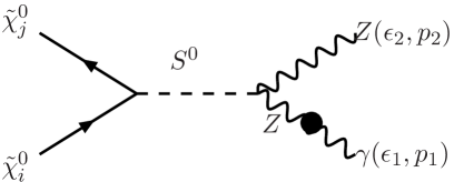
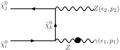
Figure 4: The needed $\gamma-Z$ self energy diagrams. The left diagram describes the s-channel exchange of $S^{0}=h^{0},~{}H^{0}$. The right diagram describes the t-channel neutralino exchange contribution, while the corresponding u-channel contribution is obtained from it through (8).

The complete set of needed diagrams consists of: the box diagrams of Fig.1, the bubbles and the initial and final triangles of Fig.2, the t-channel triangle diagrams of Fig.3, and the $\gamma-Z$ self energy contributions in Fig.4. In all cases, the full internal lines denote fermionic exchanges, the broken lines scalars, and the wavy ones gauge bosons, while the arrowed broken lines denote the usual FP ghosts. The external momenta and the polarization vectors of the outgoing gauge bosons are indicated in parentheses, in the figures.

Taking advantage of the Majorana nature of the neutralinos, the direction of the fermionic line is always chosen from $\tilde{\chi}^{0}_{i}$ to $\tilde{\chi}^{0}_{j}$; so that the wave functions of $\tilde{\chi}^{0}_{i}$ ($\tilde{\chi}^{0}_{j}$) are respectively described by positive (negative) energy Dirac solutions.

We next enumerate the main steps of the calculation.

We call the first 10 boxes in Fig.1 ”direct”. The contribution of the corresponding boxes with $\gamma\leftrightarrow Z$ exchanged, is then determined from them, by enforcing (2). Therefore, to

$$F^{ij}_{\lambda_{1},\lambda_{2};\mu_{1},\mu_{2}}(\theta)^{\rm direct~{}Box}~{}~{},$$ (4)

we should add

$$(-1)^{(\mu_{1}-\mu_{2})}F^{ji}_{\lambda_{2},\lambda_{1};\mu_{1},\mu_{2}}(\pi-\theta)^{\rm direct~{}Box}~{},$$ (5)

to take into account the $(\gamma-Z)$-crossing contribution; thereby greatly facilitating the computation.

The last 8 boxes in Fig.1, called ”twisted”, have been checked to satisfy (2) by themselves. This is also true for the bubble and initial and final triangle diagrams of Fig.2.

The third set of needed diagrams consists of the t-channel triangles of Fig.3, whose contribution we denote as

$$F^{ij}_{\lambda_{1},\lambda_{2};\mu_{1},\mu_{2}}(\theta)^{\rm t-triangle}~{}.$$ (6)

To this we should add the contribution of the corresponding u-channel triangles, obtained by interchanging $\tilde{\chi}^{0}_{i}\leftrightarrow\tilde{\chi}^{0}_{j}$, (with the arrows always running from $\tilde{\chi}^{0}_{i}$ to $\tilde{\chi}^{0}_{j}$) in Fig.3. By enforcing (2), these u-channel triangle contribution is given by

$$F^{ij}_{\lambda_{1},\lambda_{2};\mu_{1},\mu_{2}}(\theta)^{\rm u-triangle}=(-1)^{(\mu_{1}-\mu_{2})}F^{ji}_{\lambda_{2},\lambda_{1};\mu_{1},\mu_{2}}(\pi-\theta)^{\rm t-triangle}.$$ (7)

Finally, the needed $\gamma-Z$ self energy contribution is is shown in Fig.4, where the left diagram describes the contribution due to s-channel exchange of $(H^{0},h^{0})$, while the right one describes the contribution induced by a t-channel neutralino exchange. Associated to this t-channel self-energy contribution, there exist a corresponding u-channel one obtained by enforcing (2) on it, through

$$F^{ij}_{\lambda_{1},\lambda_{2};\mu_{1},\mu_{2}}(\theta)^{\rm u-{\rm self~{}energy}}=(-1)^{(\mu_{1}-\mu_{2})}F^{ji}_{\lambda_{2},\lambda_{1};\mu_{1},\mu_{2}}(\pi-\theta)^{\rm t-{\rm self~{}energy}}.$$ (8)

To summarize, the complete helicity amplitudes are given by the sum of the contributions of the diagrams in Figs.1-4, together with the contributions appearing in (5, 7, 8 ).

As already said, the $F^{ij}_{\lambda_{1},\lambda_{2};\mu_{1},\mu_{2}}(\theta)$ amplitudes are expressed analytically in terms of the PV functions. We have made several tests on these results, in order to eliminate, as much as possible, the possibility of errors. These, we enumerate below:

Requiring (2) for the contributions of each of the 8 twisted boxes in Fig.1 and of the diagrams of Fig.2, already provides generally stringent tests of their correctness.

Moreover, for the 10 direct boxes and the first four twisted boxes in Fig.1, which are similar to the box diagrams contributing to the $\gamma\gamma$-amplitudes [6], we have checked that the $\gamma Z$ diagrams smoothly go to the $\gamma\gamma$ ones, as $p_{2}^{2}\to 0$ and the $Z$ couplings are replaced by the photon ones.

The calculation of the 10 direct boxes of Fig.1, and of the t-channel triangles of Fig.3, for which no symmetry constraint is available, has been checked several times.

Finally, we have also checked that our results respect the correct helicity conservation (HC) properties at high energy and fixed angles [15]. Such tests check stringently the mass-independent high energy contributions for both transverse-$Z$ and longitudinal-$Z$ amplitudes. Any seemingly innocuous misprint, could not only violate HC, but also transform the expected logarithmic energy dependence of the dominant amplitudes at high energy, to a linear or quadratic rising with energy, thereby supplying a clear signal of error. We have had ample experience of this, during our checks.

In addition to these, we have, of course, assured that all UV divergences, as well as any scale dependence, cancel out exactly in the amplitudes, and that (3) is respected, for real MSSM parameters.

We next turn to the quantities needed for DM studies of the process (1). These are expressed in terms of the helicity amplitudes as

$$\Sigma_{ij}\equiv v_{ij}\cdot\sigma_{ij}\simeq\frac{s-m_{Z}^{2}}{64\pi[s^{2}-(m_{i}^{2}-m_{j}^{2})^{2}]}\Bigg{\{}\int_{-1}^{+1}d\cos\theta\sum_{\lambda_{1}\lambda_{2}\mu_{1}\mu_{2}}|F_{\lambda_{1}\lambda_{2}\mu_{1}\mu_{2}}^{ij}|^{2}\Bigg{\}}_{s}~{}~{},$$ (9)

where $v_{ij}$ describes the relative velocity of the $\tilde{\chi}^{0}_{i}\tilde{\chi}^{0}_{j}$-pair, implying

$$s\simeq \equiv (m_{i}+m_{j})^{2}+m_{i}m_{j}\Bigg{[}v_{ij}^{2}+v_{ij}^{4}\Big{(}\frac{3}{4}-\frac{2m_{i}m_{j}}{(m_{i}+m_{j})^{2}}\Big{)}$$ (10)

$$+ v_{ij}^{6}~{}\frac{5(m_{i}^{4}+m_{j}^{4})-12m_{i}m_{j}(m_{i}^{2}+m_{j}^{2})+22m_{i}^{2}m_{j}^{2}}{8(m_{i}+m_{j})^{4}}\Bigg{]}~{}~{},$$

up to ${\cal O}(v_{ij}^{6})$ terms. A numerical search indicates that for $v_{ij}\lesssim 0.7$, the terms up to ${\cal O}(v_{ij}^{4})$ in (10) should be adequate.

The transverse part $\Sigma_{ij}^{TT}$ of $\Sigma_{ij}$ is obtained by discarding the $\mu_{2}=0$ (longitudinal Z) contributions in the helicity summation in (9).

3 Results and comparisons

For understanding DM observations from neutralino-neutralino annihilation to $\gamma Z$ in e.g. the center of our Galaxy or in nearby galaxies like Draco [16], the quantity $\Sigma_{ij}$ (9) should be known at $v_{ij}\simeq 10^{-3}$ [1]. At so small velocities, the relative orbital angular momentum of the $\tilde{\chi}^{0}_{i}\tilde{\chi}^{0}_{j}$-pair must vanish, and the system must be in either an ${}^{1}S_{0}$ or an ${}^{3}S_{1}$ state. In such cases, the angular distribution of $d\Sigma_{ij}/d\cos\theta$ is flat.

Angular momentum conservation implies that the ${}^{1}S_{0}$ state can only contribute to transverse helicities for both $\gamma$ and $Z$; while the ${}^{3}S_{1}$ state can also give non-vanishing longitudinal-Z contributions.

Table 1: Results for $\Sigma_{ij}\equiv v_{ij}\sigma(\tilde{\chi}^{0}_{i}\tilde{\chi}^{0}_{j}\to\gamma Z)$ at $v_{ij}=0$ and $v_{ij}=0.5$, summing over all $\gamma Z$ polarizations. The transverse $Z$ contributions $\Sigma_{ij}^{TT}$ are also indicated in parentheses, for the relevant cases of either $i\neq j$ or $v_{ij}\neq 0$. Previous results for $i=j=1$ from [5] at $v_{11}=0$, and from [12] at $v_{11}=0$ and $v_{11}=0.5$, are also compared. Inputs are at the electroweak scale using the model sample of [12], with $\tan\beta=10$, and $A_{f}=0$ apart from $A_{t}=-0.3TeV$ for $m_{\tilde{f}_{L,R}}=0.8TeV$ and $A_{t}=0$ for $m_{\tilde{f}_{L,R}}=10TeV$; all masses in TeV.

	Sugra	nSugra	higgsino-1	higgsino-2	wino-1	wino-2
$M_{1}$	0.2	0.1	0.5	20	0.5	20.0
$M_{2}$	0.4	0.4	1.0	40.	0.2	4.0
$\mu$	1.0	1.0	0.2	4.0	1.0	40.0
$M_{A}$	1.0	1.0	1.0	10.0	1.0	10.0
$m_{\tilde{f}}$	0.8	0.8	0.8	10.0	0.8	10.0
$v_{11}\sigma(\tilde{\chi}^{0}_{1}\tilde{\chi}^{0}_{1}\to\gamma Z)$ in units of $10^{-27}cm^{3}sec^{-1}$; $v_{11}=0$
	$2.01\cdot 10^{-5}$	$2.60\cdot 10^{-6}$	0.224	0.0266	12.6	10.1
[12]	$2.03\cdot 10^{-5}$	$2.61\cdot 10^{-6}$	0.219	0.0220	11.7	10.1
[5]	$1.42\cdot 10^{-5}$	$1.79\cdot 10^{-6}$	0.261	0.0329	11.7	10.1
$v_{11}=0.5$
	$2.45\cdot 10^{-5}$	$5.28\cdot 10^{-6}$	0.307	0.0165	14.2	0.575
	$(2.03\cdot 10^{-5})$	$(5.16\cdot 10^{-6})$	(0.307)	(0.0165)	(14.2)	(0.575)
[12]	$2.45\cdot 10^{-5}$	$3.67\cdot 10^{-6}$	0.299	0.0166	14.2	0.576
$v_{ij}\sigma(\tilde{\chi}^{0}_{i}\tilde{\chi}^{0}_{j}\to\gamma Z)$ in units of $10^{-27}cm^{3}sec^{-1}$; $v_{ij}=0$
$\tilde{\chi}^{0}_{1}\tilde{\chi}^{0}_{2}$	$2.63\cdot 10^{-4}$	$9.64\cdot 10^{-5}$	$1.11\cdot 10^{-3}$	$3.28\cdot 10^{-5}$	$2.57\cdot 10^{-3}$	$1.04\cdot 10^{-5}$
	$(1.94\cdot 10^{-4})$	$(6.02\cdot 10^{-5})$	$(4.12\cdot 10^{-5})$	$(1.81\cdot 10^{-8})$	$(1.07\cdot 10^{-3})$	$(8.65\cdot 10^{-7})$
$\tilde{\chi}^{0}_{1}\tilde{\chi}^{0}_{3}$	$4.51\cdot 10^{-3}$	$4.46\cdot 10^{-3}$	$1.59\cdot 10^{-2}$	$4.53\cdot 10^{-4}$	0.632	2.90
	$(1.06\cdot 10^{-4})$	$(1.06\cdot 10^{-4})$	$(9.93\cdot 10^{-3})$	$(2.59\cdot 10^{-7})$	$(6.25\cdot 10^{-3})$	$(1.24\cdot 10^{-6})$
$v_{ij}=0.5$
$\tilde{\chi}^{0}_{1}\tilde{\chi}^{0}_{2}$	$2.78\cdot 10^{-4}$	$1.02\cdot 10^{-4}$	$9.11\cdot 10^{-4}$	$1.45\cdot 10^{-8}$	$2.45\cdot 10^{-3}$	$9.01\cdot 10^{-7}$
	$(2.06\cdot 10^{-4})$	$(6.15\cdot 10^{-5})$	$(3.53\cdot 10^{-5})$	$(3.98\cdot 10^{-11})$	$(1.05\cdot 10^{-3})$	$(8.93\cdot 10^{-7})$
$\tilde{\chi}^{0}_{1}\tilde{\chi}^{0}_{3}$	$4.32\cdot 10^{-3}$	$4.29\cdot 10^{-3}$	$1.54\cdot 10^{-2}$	$3.84\cdot 10^{-4}$	1.44	$5.56\cdot 10^{-2}$
	$(1.10\cdot 10^{-4})$	$(8.34\cdot 10^{-5})$	$(9.72\cdot 10^{-3})$	$(2.25\cdot 10^{-7})$	$(4.39\cdot 10^{-3})$	$(1.31\cdot 10^{-7})$

If the two neutralinos happen to be identical, Fermi statistics only allows the ${}^{1}S_{0}$-state at vanishing relative velocities, so that $\gamma$ and $Z$, are both transverse. At higher velocities though, like e.g. $v_{ii}=0.5$, longitudinal-Z amplitudes can also arise.

On the other hand, if $i\neq j$, longitudinal-Z amplitudes can also contribute, even for vanishing relative velocities.

We also note that for $i=j$, the angular structure of $d\Sigma_{ij}/d\cos\theta$, at non-negligible relative velocities, is always forward-backward symmetric. But for $i\neq j$, this is not true any more. Depending on the content of the two neutralinos, $d\Sigma_{ij}/d\cos\theta$ is sometimes peaked in the forward region, and others in the backward; compare (2). For $v_{ij}\lesssim 0.5$, $d\Sigma_{ij}/d\cos\theta$ was found to be flat, in all examples we have considered.

Next, we turn to the specific features of our approach based on the PV functions, whose definition is known to be singular close to threshold and at the forward or backward angles [17]. Thus, for relative velocities of $v_{ij}\simeq 10^{-3}$, or for angles in the forward or backward region, extrapolations must be done. In all examples we have considered, these were very smooth, with no suggestion of a possible introduction of errors.

The herewith released code PLATONdmZ calculates $d\Sigma_{ij}/d\cos\theta$ in fb [11], for real MSSM parameters at the electroweak scale, and fixed values of the relative neutralino velocity $v_{ij}$, and $\cos\theta$ using [17]. For $0.1\lesssim v_{ij}\lesssim 0.7$ and angles away from the forward and backward regions, the direct use of the code usually runs without problems.

The only known exception appears in cases where the sum of the masses of the two annihilating neutralinos happens to be close to the Z-pole. Such additional threshold singularities are specific for the $\tilde{\chi}^{0}_{i}\tilde{\chi}^{0}_{j}\to\gamma Z$ mode, and they have no counterpart in the corresponding $\gamma\gamma$- and $gg$ calculations of [6].

The next step is to compare our work, with that of other authors’. The only preexisting results in the literature apply to i=j=1 for $v_{11}=0$ and $v_{11}=0.5$, presented by [12], and for $v_{11}=0$ presented by [5]. To compare with them, we give in Table 1 the results of the PLATONdmZ code, together with those of [12] and [5]. We use the same sample of models as in [12]. These models, whose electroweak scale parameters are indicated in Table 1, have been named Sugra, nSugra, higgsino-1, higgsino-2, wino-1 and wino-2 by [12]. In Sugra and nSugra, the lightest neutralino (LSP) is a bino. In higgsino-1 and higgsino-2, the two lightest neutralinos are almost or exactly degenerate higgsinos. Finally, in wino-1 and wino-2, the lightest supersymmetric particle (LSP) is a wino, while the NLSP is a bino.

As seen in Table 1, the PLATONdmZ results for i=j=1 and $v_{11}=0$, perfectly agree with those of [12], while they deviate from those of [5]. As expected, $Z$ is completely transverse, in this case.

For $v_{11}=0.5$ though, longitudinal-Z contributions, are also possible. Because of this, in Table 1, we first give the results for the full $\gamma Z$-production, while in parentheses, in the next line, the completely transverse $\gamma Z$ production is also indicated. As shown in this Table, appreciable longitudinal Z contribution at $v_{11}=0.5$, only appears for Sugra.

At $v_{11}=0.5$, important discrepancies between our predictions for $\Sigma_{11}$ and those of [12], only appear for nSUGRA, reaching the 40% level.

We also note that in nSugra and wino-2, $\Sigma_{11}$ is very sensitive to the relative velocity $v_{11}$. This can be inferred from the big difference between the $v_{11}=0$ and $v_{11}=0.5$ results, for $i=j=1$, in these models. For nSugra this is also elucidated in Table 2. Is this sensitivity partly responsible for the discrepancy in Table 1, of the present results, with respect to those of [12]? And then, why it does not induce any discrepancy in wino-2?

Table 2: Sensitivity of $\Sigma_{11}\equiv v_{11}\cdot\sigma_{11}$ to $v_{11}$ in nSugra.

nSugra
$v_{11}$	$\Sigma_{11}$ $(10^{-27}cm^{3}sec^{-1})$
0.09	$2.65\cdot 10^{-6}$
0.2	$3.03\cdot 10^{-6}$
0.3	$3.61\cdot 10^{-6}$
0.5	$5.28\cdot 10^{-6}$

In Table 1 we also give results for $\Sigma_{12}$ and $\Sigma_{13}$ for the above 6 models, at $v_{ij}=0$ and $v_{ij}=0.5$. In parentheses, the purely transverse $\gamma Z$ contributions are also indicated, which are generally not identical to the total cross sections. Longitudinal Z production is often important in these cases, and sometimes it even dominates the transverse Z contribution, at both shown velocities.

It is also amusing to notice from Table 1 the sensitivities of $\Sigma_{12}$ and $\Sigma_{13}$ on $v_{ij}$, as it changes from 0.0 to 0.5, in the various models. For e.g. $\Sigma_{12}$, strong sensitivity appears in the higgsino-2 and wino-2 cases; while for $\Sigma_{11}$ a corresponding phenomenon is observed for nSUGRA and wino-2 again.

4 Conclusions and Outlook

The neutralinos may be the most abundant particles in the Universe, if they really turn out to contribute appreciably to its Dark Matter. They are thus, very interesting objects. In addition to this, they are very interesting from the particle physics point of view, since their Majorana nature allows them to interact in many more ways, than the ordinary (neutral) Dirac fermions. Because of this, detailed studies of their properties, both, in astrophysical observations and accelerator experiments are welcomed.

Through the present paper, an extensive analytical study of the 1-loop neutralino amplitudes in any unconstrained minimal supersymmetric model (MSSM) with real parameters, has been completed, and the related FORTRAN codes have been released [11].

More explicitly, the DM relevant process

$$\tilde{\chi}^{0}_{i}\tilde{\chi}^{0}_{j}\to\gamma Z~{},$$ (11)

has been studied analytically here, for any kinematic configuration, while

$$\tilde{\chi}^{0}_{i}\tilde{\chi}^{0}_{j}\to\gamma\gamma~{},$$ (12)

has been presented in [6], following the same spirit. The reverse process $\gamma\gamma\to\tilde{\chi}^{0}_{i}\tilde{\chi}^{0}_{j}$, which is suitable for a $LC_{\gamma\gamma}$ collider study, has appeared in [8]; while the LHC production processes, containing two or one neutralino, have appeared in [9] and [10] respectively.

The formalism of all these 1-loop processes is quite common, while the couplings are, of course, different in each case. Thus, the 1-loop Feynman diagrams determining the amplitudes for neutralino production at LHC, constitute a subset of those entering $\tilde{\chi}^{0}_{i}\tilde{\chi}^{0}_{j}\to\gamma\gamma$ production, which in turn comprise a subset of those needed for $\tilde{\chi}^{0}_{i}\tilde{\chi}^{0}_{j}\to\gamma Z$.

The latter, determines also the ”reverse” process

$$\gamma+e^{\mp}\to\tilde{\chi}^{0}_{i}+\tilde{\chi}^{0}_{j}+e^{\mp}~{},$$ (13)

where an off-shell intermediate $\gamma$ or $Z$, emitted by the incoming $e^{\mp}$-line, interacts with another incoming photon, producing a pair of neutralinos. Such a process could be studied in a future $e^{\mp}\gamma$ Linear Collider, providing further constraints on neutralinos and DM. It is straightforward to get the amplitudes for (13), from those of the process (11), studied here. We hope to present results for this in the future.

It would be really thrilling, if we ever unambiguously identify energetic $\gamma$-rays coming from Space and being associated to Dark Matter annihilation [16]. It would be even more so, if, along with the continuous $\gamma$-spectrum, we could also detect the sharp monochromatic photons implied by (12, 11). But even if this turns out to be the case, the neutralino DM interpretation will not be sufficiently convincing, unless detailed accelerator studies confirm it. The present work contributes towards this.

Acknowledgments:
We are grateful to Fawzi Boudjema for important remarks related to the comparison of our work with that of ref.[12]. GJG gratefully acknowledges also the support from the European Union program MRTN-CT-2004-503369.

Figure 1: Box Feynman diagrams needed for $\chi^{0}_{i}\chi^{0}_{j}\to\gamma Z$. Full internal lines denote fermionic exchanges, broken lines with no arrows describe scalars, and wavy lines gauge bosons. The external momenta and the polarization vectors of the outgoing gauge bosons are indicated in parentheses. The direction of the fermionic line is always from $\tilde{\chi}^{0}_{i}$ to $\tilde{\chi}^{0}_{j}$. We call the first 10 boxes ”direct”. The corresponding boxes with $\gamma\leftrightarrow Z$ exchanged, are determined by simply enforcing (2), to the above ”direct” contribution; see text. The remaining 8 boxes, called ”twisted”, automatically satisfy (2).

Figure 2: The bubble, initial and final triangle diagrams for $\chi^{0}_{i}\chi^{0}_{j}\to\gamma Z$. The exchanges are as in Fig.1, but some specific exchanges of $W$ and goldstone bosons $G$ in the bubbles, are indicated explicitly. $S^{0}$ denotes $h^{0}$ or $H^{0}$, except in the middle diagram of the last line where it also describes the exchanges of $A^{0}$ and $G^{0}$. $S$ denotes a charged scalar particle exchange. The left triangular graph in the last line describes the FP ghost contribution. These contributions satisfy (2).

Figure 3: t-channel triangles. The exchanges are as in Fig.1. The u-channel triangle contribution is obtained from it through (7); see text.

References

- [1] D.N. Spergel et.al.arXiv:astro-ph/0302209; G. Jungman, M. Kamionkowski and K. Griest, Phys. Rept. :195 (1996); M. Kamionkowski, hep-ph/0210370; M. Drees, Pramana 51,87(1998); M.S. Turner, J.A. Tyson, astro-ph/9901113, Rev. Mod. Phys. :145(1999); M.M. Nojiri, hep-ph/0305192; M. Drees hep-ph/0210142; D.P. Roy, Acta Phys. Polon. :3417 (2003) , hep-ph/0303106; F.E. Paige, hep-ph/0307342, hep-ph/0211017; J.A. Aguilar-Saavedra et.al., SPA project, hep-ph/0511344; D. Fargion, R. Konoplich, M. Grossi and M.Yu.Khlopov, Astropart. Phys. :307 (2000), astro-ph/9902327.
- [2] For a recent review see e.g. G. Lazarides, hep-ph/0601016.
- [3] G. Bertone, D. Hooper, J. Silk, Phys. Rept. :279 (2005), hep-ph/0404175; J.L. Feng, hep-ph/0405215.
- [4] L. Bergström and P. Ullio, Nucl. Phys. :27 (1997), hep-ph/9706232; Z. Bern, P. Gondolo and M. Perelstein, Phys. Lett. :86 (1997), hep-ph/9706538].
- [5] P. Ullio and L. Bergström, Phys. Rev. :1962 (1998).
- [6] G.J. Gounaris, J. Layssac, P.I. Porfyriadis and F.M. Renard, Phys. Rev. :075007 (2004), hep-ph/0309032.
- [7] G. Passarino and M. Veltman Nucl. Phys. :151 (1979).
- [8] G.J. Gounaris, J. Layssac, P.I. Porfyriadis and F.M. Renard, Eur. Phys. J. :561 (2004), hep-ph/0311076.
- [9] G.J. Gounaris, J. Layssac, P.I. Porfyriadis and F.M. Renard, Phys. Rev. :033011 (2004), hep-ph/0404162.
- [10] G.J. Gounaris, J. Layssac, P.I. Porfyriadis and F.M. Renard, Phys. Rev. :075012 (2005), hep-ph/0411366.
- [11] PLATON codes can be downloaded from http://dtp.physics.auth.gr/platon/
- [12] F. Boudjema, A. Semenov and D. Temes, Phys. Rev. :055024 (2005), hep-ph/0507127.
- [13] M. Jacob and G.C. Wick, Annals of Phys. :404 (1959), Annals of Phys. :774 (2000).
- [14] See e.g. G.J. Gounaris, C. Le Mouël and P.I. Porfyriadis, Phys. Rev. :035002 (2002), hep-ph/0107249.
- [15] G.J. Gounaris and F.M. Renard, Phys. Rev. Lett. :131601 (2005), hep-ph/0501046; G.J. Gounaris hep-ph/0510061; G.J. Gounaris and F.M. Renard, in preparation.
- [16] W. de Boer, hep-ph/0508108; L. Bergström and D. Hooper, hep-ph/0512317; S. Profumo and M. Kamionkowski, astro-ph/0601249; Y. Mambrini and E. Nezri, hep-ph/0507263; Y. Mambrini, C. Muñoz, E. Nezri and F. Prada, hep-ph/0506204.
- [17] T. Hahn, LoopTools, http://www.fsf.org/copyleft/lgpl.html; T. Hahn and M. Pérez-Victoria, hep-ph/9807565; G.J. van Oldenborgh and J.A.M. Vermaseren, Z. f. Phys. :425 (1990).