Recoilless Resonant Absorption of Monochromatic Neutrino Beam for Measuring $\Delta m^{2}_{31}$ and $\theta_{13}$

Abstract

We discuss, in the context of precision measurement of $\Delta m^{2}_{31}$ and $\theta_{13}$, physics capabilities enabled by the recoilless resonant absorption of monochromatic antineutrino beam enhanced by the Mössbauer effect recently proposed by Raghavan. Under the assumption of small relative systematic error of a few tenth of percent level between measurement at different detector locations, we give analytical and numerical estimates of the sensitivities to $\Delta m^{2}_{31}$ and $\sin^{2}2\theta_{13}$. The accuracies of determination of them are enormous; The fractional uncertainty in $\Delta m^{2}_{31}$ achievable by 10 point measurement is 0.6% (2.4%) for $\sin^{2}2\theta_{13}=0.05$, and the uncertainty of $\sin^{2}2\theta_{13}$ is 0.002 (0.008) both at 1$\sigma$ CL with the optimistic (pessimistic) assumption of systematic error of 0.2% (1%). The former opens a new possibility of determining the neutrino mass hierarchy by comparing the measured value of $\Delta m^{2}_{31}$ with the one by accelerator experiments, while the latter will help resolving the $\theta_{23}$ octant degeneracy.

I Introduction

Recently, an intriguing possibility was suggested by Raghavan raghavan1 ; raghavan2 that the resonant absorption reaction mikaelyan

$$\bar{\nu_{e}}+^{3}\text{He}+\text{orbital e}^{-}\rightarrow^{3}\text{H}$$ (1)

with simultaneous capture of an atomic orbital electron can be dramatically enhanced. The key idea is to use monochromatic $\bar{\nu_{e}}$ beam with the energy 18.6 keV from the inverse reaction ${}^{3}\text{H}\rightarrow\bar{\nu_{e}}+$${}^{3}\text{He}+\text{orbital e}^{-}$, by which the resonance condition is automatically satisfied. (See visscher ; schiffer for earlier suggestions.) He then suggested an experiment to measure $\theta_{13}$ by utilizing the ultra low-energy monochromatic $\bar{\nu_{e}}$ beam. Though similar to the reactor $\theta_{13}$ experiments krasnoyarsk ; MSYIS ; reactor_white , the typical baseline length is of order 10 m due to much lower energy of the beam by a factor of $\simeq$150, making it doable in the laboratories. The mechanism, in principle, would work with more generic setting in which ${}^{3}\text{H}$ and ${}^{3}\text{He}$ in (1) are replaced by nuclei A(Z) and A(Z-1).

The author of Ref. raghavan1 ; raghavan2 then went on to even more aggressive proposal of enhancement by a factor of $\sim 10^{11}$ by embedding both ${}^{3}\text{H}$ and ${}^{3}\text{He}$ into solids visscher ; schiffer by which the broadening of the beam due to nuclear recoil is severely suppressed by a mechanism similar to the Mössbauer effect messbauer . Then, the event rate of the $\theta_{13}$ experiment is enhanced by the same factor, allowing extremely high counting rate. Thanks to the ultimate energy resolution of $\Delta E_{\nu}/E_{\nu}\simeq 2\times 10^{-17}$ enabled by the recoilless mechanism, he was able to propose a table top experiment to measure gravitational red shift of neutrinos, a neutrino analogue of the Pound-Rebka experiment for photons pound .

In this paper, we examine possible physics potentials of the $\theta_{13}$ experiment proposed in raghavan1 ; raghavan2 . The characteristic feature of the experiment, which clearly marks the difference from the reactor $\theta_{13}$ measurement, is the use of monochromatic beam apart from the shorter baseline by a factor of $\simeq$150. Then, the most interesting question is how accurately $\Delta m^{2}_{31}$ can be determined. Note that even without recoilless setting, the beam energy width is of the order of $\Delta E_{\nu}/E_{\nu}\sim 10^{-5}$, and it can be ignored for all practical purposes. It is also interesting to explore the accuracy of $\theta_{13}$ measurement. In addition to possible extremely high statistics, the baseline as short as $\sim$10 m should allow us to utilize the setting of continuously movable detector, the one which once proposed in a reactor $\theta_{13}$ experiment movable but the one that did not survive in the (semi-) final proposal. The method will greatly help to reduce the experimental systematic uncertainties of the measurement.

We will show in our analysis that the accuracies one can achieve for $\Delta m^{2}_{31}$ and $\theta_{13}$ determination by the recoilless resonant absorption are enormous. At $\sin^{2}2\theta_{13}=0.05$, for example, the fractional uncertainty in $\Delta m^{2}_{31}$ determination is 0.6% (2.4%) and the uncertainty of $\sin^{2}2\theta_{13}$ is 0.002 (0.008) both at 1$\sigma$ CL under an optimistic (pessimistic) assumption of systematic error of 0.2% (1%).

What is the scientific merit of such precision measurement of $\Delta m^{2}_{31}$ and $\theta_{13}$? With a 1% level precision of $\Delta m^{2}_{31}$, the method for determining neutrino mass hierarchy by comparing between the two effective $\Delta m^{2}$ measured in reactor and accelerator (or atmospheric) disappearance measurement NPZ ; GJK would work, opening another door for determining the neutrino mass hierarchy. It is also proposed MSYIS that the $\theta_{23}$ octant degeneracy can be resolved by combining reactor measurement of $\theta_{13}$ with accelerator disappearance (appearance) measurement of $\sin^{2}2\theta_{23}$ ($s^{2}_{23}\sin^{2}2\theta_{13}$). (See octant ; gouvea for earlier qualitative suggestions.) The results of the recent quantitative analysis resolve23 , however, indicate that the resolving power of the method is limited at small $\theta_{13}$ primarily because of the uncertainties in reactor measurement of $\theta_{13}$. Therefore, the highly accurate measurement of $\Delta m^{2}_{31}$ and $\theta_{13}$ which is enabled by using the resonant absorption reaction should help resolving the mass hierarchy and the $\theta_{23}$ degeneracies.

In Sec. II, we discuss “conceptual design” of the possible experiments. In Sec. III, we define the statistical method for our analysis. In Sec. IV, we present numerical analysis of the sensitivities of $\theta_{13}$ and $\Delta m^{2}_{31}$ measurement. In Sec. V, we complement the numerical estimate in Sec. IV by giving analytic estimate of the sensitivities. In Sec. VI, we give some remarks on implications of our results. In Appendix A, we give a general formula for the inverse of the error matrix.

II Which kind of $\theta_{13}$ experiment?

We give preliminary discussions on which kind of setting is likely to be the best one for experiment to measure $\Delta m^{2}_{31}$ and $\theta_{13}$ with use of ultra low-energy monochromatic $\bar{\nu_{e}}$ beam. In this section, we rely on the one-mass scale dominant one-mass (or the two-flavor) approximation of the neutrino oscillation probability $P(\bar{\nu_{e}}\rightarrow\bar{\nu_{e}})$, though we use the full three-flavor expression in our quantitative analysis performed in Sec. IV. It reads

$$P(\bar{\nu_{e}}\rightarrow\bar{\nu_{e}})=1-\sin^{2}2\theta_{13}\sin^{2}{\left(\frac{\Delta m^{2}_{31}L}{4E}\right)},$$ (2)

where the neutrino mass squared difference is defined as $\Delta m^{2}_{ji}\equiv m^{2}_{j}-m^{2}_{i}$ with neutrino masses $m_{i}$ ($i$ = 1 - 3) and $L$ is a distance from a source to a detector. With $E_{\nu}=18.6$ keV, the first oscillation maximum (minimum in $P(\bar{\nu_{e}}\rightarrow\bar{\nu_{e}})$) is reached at the baseline distance

$$L_{\text{\text{OM}}}=9.2\left(\frac{\Delta m^{2}_{31}}{2.5\times 10^{-3}\text{eV}^{2}}\right)^{-1}\text{m}.$$ (3)

While the current value of $\Delta m^{2}_{31}$ which comes from the atmospheric SKatm and the accelerator K2K measurement has large uncertainties, it should be possible to narrow down the value thanks to the ongoing and the forthcoming disappearance measurement by MINOS MINOS and T2K JPARC experiments. Furthermore, the experiment considered in this paper is powerful enough to determine both quantities accurately at the same time, if detector locations are appropriately chosen.

The whole discussion of the $\theta_{13}$ experiment must be preceded by the test measurement at $\sim$10 cm or so to verify the principle, namely to demonstrate that the mechanism of resonant enhancement proposed in raghavan1 ; raghavan2 is indeed at work. At the same time, the flux times cross section must be measured to check the consistency of the Monte Carlo estimate. Then, one can go on to the measurement of $\theta_{13}$ and $\Delta m^{2}_{31}$, and possibly other quantities. Because of the expected high statistics of the experiment it is natural to think about using spectrum informations. In the case of monochromatic beam it amounts to consider measurement at several different detector locations.

Let us estimate the event rate. Although the precise rate is hard to estimate, the numbers displayed below will give the readers a feeling on what would be the time scale for the experiment. The $\bar{\nu_{e}}$ flux from ³H source with strength $S$ MCi due to bound state beta decay is given by

$$f_{\bar{\nu_{e}}}=1.4\times 10^{7}\left(\frac{S}{1\text{MCi}}\right)\left(\frac{L}{10~{}\text{m}}\right)^{-2}\text{cm}^{-2}\text{s}^{-1}$$ (4)

where the ratio of bound state beta decay to free space decay is taken to be $4.7\times 10^{-3}$ based on bahcall . The rate of the resonant absorption reaction can be computed by using cross section $\sigma_{res}$ and number of target atoms $N_{T}$ as $R=N_{T}f_{\bar{\nu_{e}}}\sigma_{res}$. Without the Mössbauer enhancement the cross section is estimated to be $\sigma_{res}\simeq 10^{-42}\text{cm}^{2}$ raghavan1 ; raghavan2 based on mikaelyan . Then, the rate with target mass $M_{T}$ without neutrino oscillation is given by

$$R=2.4\times 10^{-4}\left(\frac{SM_{T}}{1\text{MCi}\cdot\text{kg}}\right)\left(\frac{L}{10~{}\text{m}}\right)^{-2}\text{day}^{-1}$$ (5)

An improved estimate in raghavan2 entailed a factor of $\simeq 10^{11}$ enhancement of the cross section by the Mössbauer effect after the source and the target are embedded into solids. Assuming the enhancement factor, $\sigma_{res}\simeq 5\times 10^{-32}\text{cm}^{2}$ and the rate becomes

$$R_{\text{enhanced}}=1.2\times 10^{4}\left(\frac{SM_{T}}{1\text{MCi}\cdot\text{g}}\right)\left(\frac{L}{10~{}\text{m}}\right)^{-2}\text{day}^{-1}$$ (6)

Therefore, one obtains about $1.2\times 10^{6}$ events per day for 1 MCi source and 100 g ³He target at a baseline distance $L=10$ m. If the enhancement factor is not reached the running time for collecting the same number of events becomes longer accordingly.

Thus, once the ³He (and much easier ³H) implementation into solid is achieved, the event rate is sufficient. The real issue for high sensitivity measurement of $\Delta m^{2}_{31}$ and $\sin^{2}2\theta_{13}$ is whether the produced ³H can be counted directly without waiting for decaying back to ³He by emitting electron. It is because the long lifetime of 12.33 year table_isotope of ³H makes it impossible to identify which period the decayed ³H was produced, resulting in the errors of the event rate in each detector location. Possibilities of real-time counting and direct counting by extracting ³H atoms are mentioned in raghavan2 . In this paper, we assume that at least one of such methods works, and it offers opportunity of direct counting of events. Note that the detection efficiency need not to be high because of huge number of events. What is important is the time-stable counting rate which allows relative systematic errors between measurement at different detector locations small enough.

III Statistical method for analysis

In this section, we define the statistical procedure for our analysis to estimate the sensitivities of $\Delta m^{2}_{31}$ and $\sin^{2}2\theta_{13}$ to be carried out in the following sections. We aim at illuminating general properties of the $\chi^{2}$ under the assumption of the small uncorrelated systematic errors compared to the correlated ones.

III.1 Definition of $\chi^{2}$ and characteristic properties of errors

We consider measurement at $n$ different distances $L=L_{i}$ ($i=1,2,...n$) from the source. Then, the appropriate form of $\Delta\chi^{2}$ which is suited for analytic study SYSHS and is simply denoted as $\chi^{2}$ hereafter, is as follows:

$$\chi^{2}=\sum_{i=1}^{n}\frac{\left[N^{obs}_{i}-(1+\alpha)N^{exp}_{i}\right]^{2}}{N^{exp}_{i}+(\sigma_{usys,i}N^{exp}_{i})^{2}}+\left(\frac{\alpha}{\sigma_{c}}\right)^{2}$$ (7)

where $N^{obs}$ is the number of events computed with the values of parameters given by nature, and $N^{exp}$ is the one computed with certain trial set of parameters. $\sigma_{c}$ is the systematic error common to measurement at $n$ different distances, the correlated error, whereas $\sigma_{usys,i}$ indicate errors that cannot be attributed to $\sigma_{c}$, the uncorrelated errors. The example of the former and the latter errors are as follows:

• $\sigma_{c}$ (correlated error): Uncertainties in number of target ³He atoms, errors in counting the number of produced tritium nuclei, errors in calculating resonant absorption cross section, errors in estimating the efficiency of counting tritium nuclei

• $\sigma_{usys,i}$ (uncorrelated error) : Possible time dependences of number of decaying tritium nuclei and detection efficiency of events

Since we consider moving detector setting the list of the thinkable uncorrelated systematic errors is quite limited. If the near detector with the identical structure with a movable far detector exists the error can, in principle, be vanishingly small. One may think of the errors of the order of 0.1%-0.3%. It is because the flux times cross section can be monitored in real time by a near detector. In fact, the similar values for uncorrelated systematic error are adopted in sensitivity estimate of some of the reactor $\theta_{13}$ experiments such as the Braidwood, the Daya Bay, and the Angra projects braidwood ; dayabay ; angra . In near future experiments, somewhat larger values are taken, 0.6% in Double-Chooz project DCHOOZ and 0.35% in KASKA KASKA .

On the other hand, it may not be so easy to control the correlated systematic error $\sigma_{c}$. The number of ³H nuclei may be measured when they are implemented into solid. The number of target nuclei times the resonant absorption cross section may be measured in a research and development stage with a near detector. Therefore, we suspect that the largest error may come from uncertainty in counting rate of the produced ³H nuclei. Of course, reliable estimate of systematic errors $\sigma_{c}$ and $\sigma_{usys}$ requires specification of the site to estimate the background caused by n³H reaction etc. But, it can be experimentally measured by the source on and off procedure, as pointed out in raghavan1 . Lacking definitive numbers for $\sigma_{c}$ at the moment, we use a tentative value $\sigma_{c}=10$% throughout our analysis. We have checked that the results barely change even if we use more conservative number $\sigma_{c}=20$%.

If the direct counting of ³H atoms does not work, we may have to expect much larger systematic errors, because one has to extract event rate at each detector location only by fitting the decay curve. In this case, determination of baseline dependent event rates would be more and more difficult for larger number of detector locations. Probably, the better strategy without the direct counting would be to place multiple identical detectors (or of the same structure) at appropriate baseline distances. Even in this case, it is quite possible that the uncorrelated systematic error $\sigma_{usys}$ can be controlled to 1% level, as expected in a variety of reactor $\theta_{13}$ experiments reactor_white .

III.2 Approximate form of $\chi^{2}$ with hierarchy in errors

By eliminating $\alpha$ through minimization the $\chi^{2}$ can be written as

$$\Delta\chi^{2}=\vec{x}^{\text{T}}V^{-1}\vec{x}$$ (8)

where $\vec{x}$ is defined as

$$\vec{x}^{\text{T}}=\left[\frac{N^{obs}_{1}-N^{exp}_{1}}{N^{exp}_{1}},\frac{N^{obs}_{2}-N^{exp}_{2}}{N^{exp}_{2}},\cdot\cdot\cdot\frac{N^{obs}_{n}-N^{exp}_{n}}{N^{exp}_{n}}\right].$$ (9)

Using the general formula given in Appendix A, $V^{-1}$ is given by

$$(V^{-1})_{ij}=\frac{\delta_{ij}}{\sigma^{2}_{ui}}-\frac{1}{\sigma^{2}_{ui}\sigma^{2}_{uj}}\frac{\sigma^{2}_{c}}{\left[1+\left(\sum_{k=1}^{n}\frac{1}{\sigma^{2}_{uk}}\right)\sigma^{2}_{c}\right]}$$ (10)

where $\sigma^{2}_{ui}\equiv\sigma^{2}_{usys,i}+\frac{1}{N^{exp}_{i}}$. By construction, the $\chi^{2}$ depends upon $\sigma_{usys,i}$ and $N^{exp}_{i}$ only through this combination. Therefore, the particular case that will be taken in the next section, in fact, includes many cases with different event number but with the same $\sigma_{u}$.

Under the approximation $\sigma^{2}_{ui}\ll\sigma^{2}_{c}$, $V^{-1}$ simplifies;

$$(V^{-1})_{ij}=\frac{\delta_{ij}}{\sigma^{2}_{ui}}-\frac{1}{\sigma^{2}_{ui}\sigma^{2}_{uj}\left(\sum_{k=1}^{n}\frac{1}{\sigma^{2}_{uk}}\right)}.$$ (11)

The remarkable feature of (11) is the “scaling behavior” in which $\chi^{2}$ is independent of the correlated error $\sigma_{c}$, and the sensitivity to $\sin^{2}\theta_{13}$ and $\Delta m^{2}_{31}$ can be made higher as the uncorrelated systematic errors as well as the statistical error become smaller. It may be counterintuitive because the leading term of the error matrix $V$ is of order $\sigma^{2}_{c}$. (See Appendix A.) It is due to the singular nature of the leading order matrix, as noted in reactorCP .

IV Estimation of sensitivities of $\Delta m^{2}_{31}$ and $\theta_{13}$

We now examine the sensitivities of $\Delta m^{2}_{31}$ and $\sin^{2}2\theta_{13}$ achievable by the recoilless resonant absorption of monochromatic $\bar{\nu}_{e}$ enhanced by the Mössbauer effect. The numerical estimate of the sensitivities in this section will be followed by the one by the analytic method in Sec. V.

The setting of movable detector and the expected high statistics of the experiment make it possible to consider the situation that an equal number of events are taken in each detector location. Of course, the far a detector from the source, the longer an exposure will take. In the following analysis, the number of events are assumed to be $10^{6}$ in each detector location. Given the rate in (6), and assuming that the direct counting works, it is obtainable in $\sim$10 days for 100 g ³He target even if the detector is located at the second oscillation maximum, $L=3L_{\text{OM}}$. On the other hand, the number of events $10^{6}$ is sufficient for our purpose because it is unlikely that the uncorrelated systematic errors can be made much smaller than 0.1%.

We take a “common-sense approach” to determine the locations of the detectors and postpone the discussion of the optimization problem. We examine the following four types of run, Run I, IIA, IIB, and III, for the measurement.

• Run I: Measurement at 5 detector positions, $L=\frac{1}{5}L_{\text{OM}},\frac{3}{5}L_{\text{OM}},L_{\text{OM}},\frac{7}{5}L_{\text{OM}}$, and $\frac{9}{5}L_{\text{OM}}$ are considered so that $\Delta\equiv\Delta m^{2}_{31}L/4E=\pi/10,3\pi/10,\pi/2,7\pi/10,9\pi/10$ are covered.

• Run IIA: A setting for precision determination of $\Delta m^{2}_{31}$ by measurement at 10 detector positions: $L=L_{i}$ ($i=1,...10$) where $L_{i+1}=L_{i}+\frac{1}{5}L_{\text{OM}}$ and $L_{1}=\frac{1}{5}L_{\text{OM}}$ so that the range $\Delta=0$ to $\pi$ is covered.

• Run IIB: A setting for precision determination of $\Delta m^{2}_{31}$ by measurement at 10 detector positions: $L=L_{i}$ ($i=1,...10$) where $L_{i+1}=L_{i}+\frac{2}{5}L_{\text{OM}}$ and $L_{1}=\frac{1}{5}L_{\text{OM}}$ so that the entire period, $\Delta=0$ to 2$\pi$, is covered.

• Run III: A setting of 20 detector positions: $L=L_{i}$ ($i=1,...20$) where $L_{i+1}=L_{i}+\frac{1}{5}L_{\text{OM}}$ and $L_{1}=\frac{1}{5}L_{\text{OM}}$ ($\Delta=0-2\pi$). It is to check the scaling behavior of the sensitivity with respect to errors.

In the following two subsections IV.1 and IV.2, we examine the cases of the optimistic ($\sigma_{usys}=0.2$%) and the pessimistic ($\sigma_{usys}=1$%) systematic errors. We stress here that the analyses we will present there contain much more general cases. For example, because of the scaling behavior discussed in the previous section, the case with $N=10^{6}$ and $\sigma_{usys}=0.2$% is equivalent to $N=2\times 10^{5}$ and $\sigma_{usys}=0.0$%. Similarly, the case with $N=10^{6}$ and $\sigma_{usys}=1$% is equivalent to $N=1.33\times 10^{4}$ and $\sigma_{usys}=0.5$%. In the last subsection IV.3, we give an estimate of the sensitivities using a tentative setting which may be possible without direct counting of ³H atoms.

IV.1 Case of optimistic systematic error

We focus in this subsection on the case of optimistic systematic error, from which one may obtain some feeling on the ultimate sensitivities achievable by the present method with the four Run options described above. As we mentioned earlier, the correlated systematic error $\sigma_{c}$ is taken to be a tentative value of 10% throughout our analysis. The uncorrelated systematic error $\sigma_{usys}$, which is assumed to be equal for all detector locations, is taken to be 0.2% in this subsection.

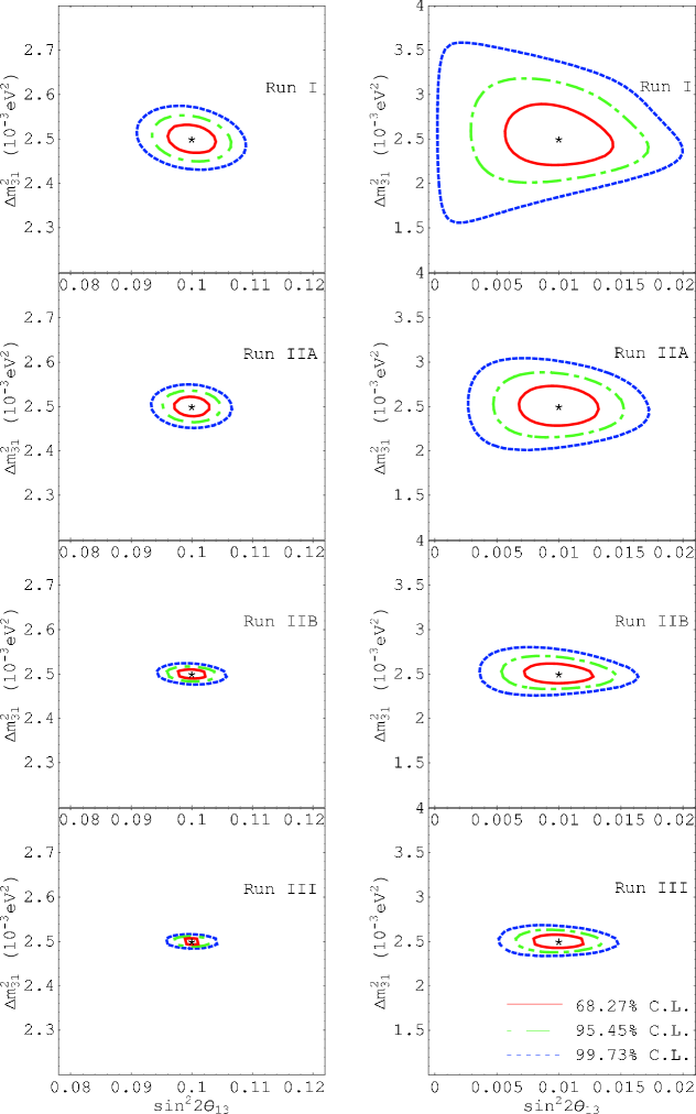
Figure 1: The expected allowed region by Run I, IIA, IIB, and III with number of events $10^{6}$ in each location are depicted. The red-solid, the green-dashed, and the blue-dotted lines are for 1$\sigma$ (68.27%), 2$\sigma$ (95.45%), and 3$\sigma$ (99.73%) CL for 2 DOF, respectively. The input values of the mixing parameters are marked by asterisks and they are as follows: $\Delta m^{2}_{31}=2.5\times 10^{-3}$ eV², $\sin^{2}2\theta_{13}=0.1$ and 0.01 in the left and the right panels.

Table 1: The expected fractional uncertainty $\delta(\Delta m^{2})/\Delta m^{2}_{31}(0)$ in % for the optimistic systematic error of $\sigma_{usys}=0.2$% reachable by the Run I$-$III defined in the text. The uncertainties are given at 1$\sigma$ (68.27%) CL for 1 DOF, and the numbers in parentheses are the ones at 3$\sigma$ (99.73%) CL for 1 DOF. In the left, middle, and right columns, the input value of $\theta_{13}$ are taken as $\sin^{2}2\theta_{13}=0.1$, 0.05, and 0.01, respectively.

$\sigma_{usys}=0.2$%	$\sin^{2}2\theta_{13}=0.1$	$\sin^{2}2\theta_{13}=0.05$	$\sin^{2}2\theta_{13}=0.01$
Run type		$\delta(\Delta m^{2})/\Delta m^{2}_{31}(0)$ (in %) at 1$\sigma$ (3$\sigma$) CL
Run I (5 locations)	0.84 (2.5)	1.7 (5.0)	9.6 $\left({}^{+31}_{-23}\right)$
Run IIA (10 locations)	0.56 (1.7)	1.2 (3.5)	6.0 $\left({}^{+18}_{-16}\right)$
Run IIB (10 locations)	0.28 (0.8)	0.56 (1.6)	2.8 $\left({}^{+9.6}_{-8.0}\right)$
Run III (20 locations)	0.2 (0.56)	0.4 (1.2)	2.0 $\left({}^{+6.0}_{-5.6}\right)$

Table 2: The expected sensitivity to the $\sin^{2}2\theta_{13}$ for the optimistic systematic error of $\sigma_{usys}=0.2$% reachable by the Run I$-$III defined in the text. The uncertainties $\delta(\sin^{2}2\theta_{13})$ are given at 1$\sigma$ (68.27%) CL for 1 DOF, and the numbers in parentheses are the ones at 3$\sigma$ (99.73%) CL for 1 DOF. In the left, middle, and right columns, the input value of $\theta_{13}$ are taken as $\sin^{2}2\theta_{13}=0.1$, 0.05, and 0.01, respectively.

$\sigma_{usys}=0.2$%	$\sin^{2}2\theta_{13}=0.1$	$\sin^{2}2\theta_{13}=0.05$	$\sin^{2}2\theta_{13}=0.01$
Run type		$\sin^{2}2\theta_{13}$ at 1$\sigma$ (3$\sigma$) CL
Run I (5 locations)	0.1 $\pm 0.0026$ (0.0078)	0.05 $\pm 0.0027$ (0.0081)	0.01 $\pm 0.0028$ (0.0085)
Run IIA (10 locations)	0.1 $\pm 0.0019$ (0.0058)	0.05 $\pm 0.0020$ (0.0061)	0.01 $\pm 0.0021$ (0.0064)
Run IIB (10 locations)	0.1 $\pm 0.0017$ (0.0050)	0.05 $\pm 0.0018$ (0.0053)	0.01 $\pm 0.0018$ (0.0055)
Run III (20 locations)	0.1 $\pm 0.0013$ (0.0038)	0.05 $\pm 0.0014$ (0.0041)	0.01 $\pm 0.0014$ (0.0042)

In Fig. 1 we show in $\sin^{2}2\theta_{13}-\Delta m^{2}_{31}$ plane the expected allowed region by Run I, IIA, IIB, and III with number of events $10^{6}$ in each location. Throughout the analysis, the true values of $\Delta m^{2}_{31}$ is assumed to be $\Delta m^{2}_{31}=2.5\times 10^{-3}$ eV². The input values of $\sin^{2}2\theta_{13}$ is taken as 0.1 and 0.01 in the left and the right panels in Fig. 1, respectively. Throughout the numerical analyses in this paper, the other oscillation parameters are taken as: $\Delta m^{2}_{21}=7.9\times 10^{-5}$ eV², $\sin^{2}\theta_{12}=0.31$, and $\sin^{2}\theta_{23}=0.5$. In each panel, the red-solid, the green-dashed, and the blue-dotted lines are for 1$\sigma$ (68.27%), 2$\sigma$ (95.45%), and 3$\sigma$ (99.73%) CL for 2 DOF (degrees of freedom), respectively.

To complement Fig. 1, we give in Table 1 the expected sensitivities to $\Delta m^{2}_{31}$ at 1$\sigma$ and 3$\sigma$ CL (the latter in parentheses) for 1 DOF for Run I-III. They are obtained by optimizing $\sin^{2}2\theta_{13}$ in the fit. For relatively large $\theta_{13}$, $\sin^{2}2\theta_{13}\raise 1.29167pt\hbox{$\;>$\kern-7.5pt\raise-4.73611pt\hbox{$\sim\;$}}0.05$ the expected sensitivities to $\Delta m^{2}_{31}$ are enormous. For $\sin^{2}2\theta_{13}=0.05$ the sensitivities are already less than 1% in Run IIA, and is about 0.6% in Run IIB both at 1$\sigma$ CL. The scaling behavior mentioned at the end of the previous section is roughly satisfied, as indicated in Table 1. (See Sec. V for more detailed discussions.) For a small value of $\theta_{13}$, $\sin^{2}2\theta_{13}=0.01$ the sensitivity to $\Delta m^{2}_{31}$ are much worse, as shown in Table 1. They are about 6% in Run IIA, and 3% in Run IIB both at 1$\sigma$ CL. If Run III is carried out it can go down to 2%.

In Table 2 the expected sensitivity to $\sin^{2}2\theta_{13}$ at 1$\sigma$ and 3$\sigma$ CL (the latter in parentheses) for 1 DOF are given. The sensitivities to $\sin^{2}2\theta_{13}$ can be better characterized by $\delta(\sin^{2}2\theta_{13})$, not its fraction to $\sin^{2}2\theta_{13}$, as will be understood in our analytic treatment in Sec. V. By Run I one can already achieve the accuracy of $\delta(\sin^{2}2\theta_{13})\simeq 0.003$, and Run IIA or IIB reach to $\delta(\sin^{2}2\theta_{13})\simeq 0.002$. The effect of measurement at multiple detector locations on improvement of the sensitivity is relatively minor in the case of sensitivities to $\sin^{2}2\theta_{13}$. This is in sharp contrast to the case of $\Delta m^{2}_{31}$.

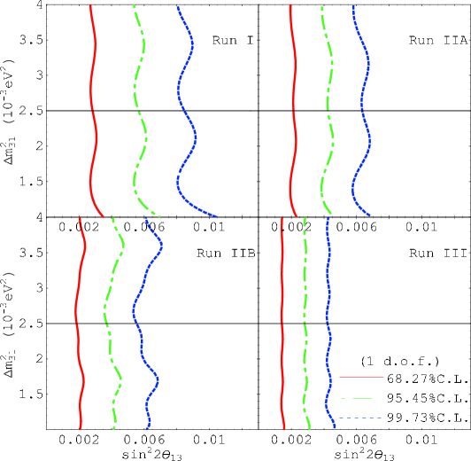
Figure 2: The sensitivity limit of $\theta_{13}$ by Run I, IIA, IIB, and III with number of events $10^{6}$ in each location are depicted. The red-solid, the green-dashed, and the blue-dotted lines are for 1$\sigma$ (68.27%), 2$\sigma$ (95.45%), and 3$\sigma$ (99.73%) CL for 1 DOF, respectively.

To show the sensitivity limit on $\theta_{13}$ achievable by the present method, we present in Fig. 2 the excluded regions in $\sin^{2}2\theta_{13}-\Delta m^{2}_{31}$ space, assuming the case of no depletion of $\bar{\nu}_{e}$ flux. The four panels in Fig. 2 correspond to Run I, IIA, IIB, and III. In each panel, the red-solid, the green-dashed, and the blue-dotted lines are for 1$\sigma$ (68.27%), 2$\sigma$ (95.45%), and 3$\sigma$ (99.73%) CL for 1 DOF, respectively. The sensitivities indicated in Fig. 2 is quite impressive, which reach to $\sin^{2}2\theta_{13}\simeq 0.006$ at 2$\sigma$ CL even in Run I, and to $\sin^{2}2\theta_{13}\simeq 0.004$ at the same CL in Run IIB. As expected the improvement by adding more detector locations is relatively minor.

IV.2 Case of pessimistic systematic error

It might be possible that we end up with the error of $\sim$1% due to, e. g., time dependence of the source even though the method of movable detector with direct counting of ³H works. In Fig. 3 we present the similar allowed region in $\sin^{2}2\theta_{13}-\Delta m^{2}_{31}$ space obtained by the same Run I, IIA, IIB, and III with the same number of events of $10^{6}$ in each location but with a pessimistic systematic error of $\sigma_{usys}=$ 1%. At large $\theta_{13}$, $\sin^{2}2\theta_{13}=0.1$, we still have reasonable sensitivities to $\Delta m^{2}_{31}$. For Run IIB and III, for example, the sensitivities are about 1-2% level for 2 DOF. At $\sin^{2}2\theta_{13}=0.01$, however, the sensitivity to $\Delta m^{2}_{31}$ is lost except for the one at 1$\sigma$ CL in Run III. It indicates that the value of $\theta_{13}$ is close to the sensitivity limit, and hence we do not place the figure for it though we did for the case of optimistic error, Fig. 2.

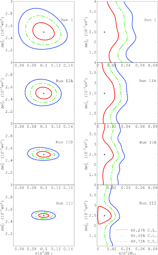
Figure 3: The same as in Fig. 1 but with the pessimistic systematic error of $\sigma_{usys}$ 1%.The input values of $\sin^{2}2\theta_{13}$ is taken as 0.1 and 0.01 in the left and the right panels.

For more detailed information on sensitivities with the pessimistic systematic error of $\sigma_{usys}=1$%, we give in Tables 3 and 4 the sensitivities at 1$\sigma$ and 3$\sigma$ CL (the latter in parentheses) for 1 DOF to $\Delta m^{2}_{31}$ and $\sin^{2}2\theta_{13}$, respectively. The column without number represents that no limit is obtained, in the similar way as seen in the right panels in Fig. 3. At relatively large $\theta_{13}$, $\sin^{2}2\theta_{13}=0.1$ and 0.05, the sensitivities to $\Delta m^{2}_{31}$ remain to be good, 1.2% and 2.4% at 1$\sigma$ CL for Run IIB. But, the sensitivity quickly drops and is about 15% in the same Run for $\sin^{2}2\theta_{13}=0.01$. The sensitivity to $\sin^{2}2\theta_{13}$ is still reasonable, $\delta(\sin^{2}2\theta_{13})\simeq 0.008$ at 1$\sigma$ CL for Run IIB even at $\sin^{2}2\theta_{13}=0.01$.

Table 3: The expected fractional uncertainty $\delta(\Delta m^{2})/\Delta m^{2}_{31}(0)$ in % for the pessimistic systematic error of $\sigma_{usys}=1$% reachable by the Run I$-$III defined in the text. The uncertainties are given at 1$\sigma$ (68.27%) CL for 1 DOF, and the numbers in parentheses are the ones at 3$\sigma$ (99.73%) CL for 1 DOF. In the left, middle, and right columns, the input value of $\theta_{13}$ are taken as $\sin^{2}2\theta_{13}=0.1$, 0.05, and 0.01, respectively. The column without number represents that no limit is obtained.

$\sigma_{usys}=1$%	$\sin^{2}2\theta_{13}=0.1$	$\sin^{2}2\theta_{13}=0.05$	$\sin^{2}2\theta_{13}=0.01$
Run type		$\delta(\Delta m^{2})/\Delta m^{2}_{31}(0)$ (in %) at 1$\sigma$ (3$\sigma$) CL
Run I (5 locations)	${}^{+4.0}_{-3.6}$ $\left({}^{+12}_{-10}\right)$	${}^{+8.0}_{-7.2}$ $\left({}^{+27}_{-20}\right)$	—
Run IIA (10 locations)	2.4 $\left({}^{+8.0}_{-7.2}\right)$	5.2 $\left({}^{+16}_{-14}\right)$	${}^{+26}_{-24}$ ( — )
Run IIB (10 locations)	1.2 (3.5)	2.4 $\left({}^{+8.4}_{-7.2}\right)$	${}^{+15}_{-12}$ ( — )
Run III (20 locations)	0.8 (2.4)	1.6 (5.2)	${}^{+9.2}_{-8.4}$ ( — )

Table 4: The expected sensitivity to the $\sin^{2}2\theta_{13}$ for the pessimistic systematic error of $\sigma_{usys}=1$% reachable by the Run I$-$III defined in the text. The uncertainties $\delta(\sin^{2}2\theta_{13})$ are given at 1$\sigma$ (68.27%) CL for 1 DOF, and the numbers in parentheses are the ones at 3$\sigma$ (99.73%) CL for 1 DOF. In the left, middle, and right columns, the input value of $\theta_{13}$ are taken as $\sin^{2}2\theta_{13}=0.1$, 0.05, and 0.01, respectively. The column without number represents that no limit is obtained.

$\sigma_{usys}=1$%	$\sin^{2}2\theta_{13}=0.1$	$\sin^{2}2\theta_{13}=0.05$	$\sin^{2}2\theta_{13}=0.01$
Run type		$\sin^{2}2\theta_{13}$ at 1$\sigma$ (3$\sigma$) CL
Run I (5 locations)	0.1 $\pm 0.011$ (0.034)	0.05 $\pm 0.012$ (0.037)	0.01 ${}^{+0.013}_{---}$ $\left({}^{+0.037}_{---}\right)$
Run IIA (10 locations)	0.1 $\pm 0.009$ (0.026)	0.05 $\pm 0.009$ $\left({}^{+0.027}_{-0.022}\right)$	0.01 ${}^{+0.009}_{---}$ $\left({}^{+0.028}_{---}\right)$
Run IIB (10 locations)	0.1 $\pm 0.007$ (0.023)	0.05 $\pm 0.008$ $\left({}^{+0.021}_{-0.024}\right)$	0.01 $\pm 0.008$ $\left({}^{+0.024}_{---}\right)$
Run III (20 locations)	0.1 $\pm 0.006$ (0.017)	0.05 $\pm 0.006$ (0.018)	0.01 $\pm 0.006$ $\left({}^{+0.019}_{---}\right)$

For disappearance measurement of $P(\bar{\nu}_{e}\rightarrow\bar{\nu}_{e})$, $\sin^{2}2\theta_{13}=0.01$ is a too small value for a pessimistic systematic error of $\sigma_{usys}=$ 1% to retain the sensitivity to $\Delta m^{2}_{31}$. Therefore, reduction of the uncorrelated systematic error is the mandatory requirement in this method for accurate measurement of $\Delta m^{2}_{31}$ at small $\theta_{13}$.

IV.3 Case without direct detection of ³H

Table 5: The expected fractional uncertainty $\delta(\Delta m^{2})/\Delta m^{2}_{31}(0)$ in %, and $\delta(\sin^{2}2\theta_{13})$ for the pessimistic systematic error of $\sigma_{usys}=1$%, 2%, and 3% reachable by Run 0 with 3 detectors as defined in the text. The uncertainties are given at 1$\sigma$ (68.27%) CL for 1 DOF, and the numbers in parentheses are the ones at 3$\sigma$ (99.73%) CL for 1 DOF. In the left, middle, and right columns, the input value of $\theta_{13}$ are taken as $\sin^{2}2\theta_{13}=0.1$, 0.05, and 0.01, respectively. The column without number represents that no limit is obtained.

Run 0	$\sin^{2}2\theta_{13}=0.1$	$\sin^{2}2\theta_{13}=0.05$	$\sin^{2}2\theta_{13}=0.01$
$\sigma_{usys}$		$\delta(\Delta m^{2})/\Delta m^{2}_{31}(0)$ (in %) at 1$\sigma$ (3$\sigma$) CL
1 %	$\left({}^{+8.6}_{-6.8}\right)$ ($\left({}^{+15}_{-13}\right)$)	$\left({}^{+12}_{-10}\right)$ (—)	— (—)
2 %	$\left({}^{+12}_{-10}\right)$ (—)	$\left({}^{+18}_{-16}\right)$ (—)	— (—)
3 %	$\left({}^{+15}_{-13}\right)$ (—)	— (—)	— (—)
$\sigma_{usys}$		$\sin^{2}2\theta_{13}$ at 1$\sigma$ (3$\sigma$) CL
1 %	0.1 $\pm 0.012$ (0.035)	0.05 $\pm 0.012$ (0.037)	0.01 ${}^{+0.013}_{---}$ $\left({}^{+0.038}_{---}\right)$
2 %	0.1 $\pm 0.022$ $\left({}^{+0.06}_{-0.07}\right)$	0.05 $\pm 0.024$ $\left({}^{+0.066}_{---}\right)$	0.01 ${}^{+0.024}_{---}$ $\left({}^{+0.069}_{---}\right)$
3 %	0.1 $\pm 0.033$ $\left({}^{+0.089}_{---}\right)$	0.05 $\pm 0.035$ $\left({}^{+0.094}_{---}\right)$	0.01 ${}^{+0.035}_{---}$ $\left({}^{+0.098}_{---}\right)$

Suppose that the direct detection of ³H in the target is not possible. Then, we may have to take the option of multiple detectors with the same structure, giving up the idea of movable detector. In this case, most probably, we have to accept a pessimistic value of the uncorrelated systematic error of 1-3%. It will cause two important changes in designing the experiment. (1) Number of events that can be accumulated in a reasonable time scale would be smaller by a factor of $\sim$10 than the case of direct detection. (2) Number of detectors that can be prepared by keeping their identity to suppress the uncorrelated systematic errors may be limited. Therefore, 3 detector setting, for example, (in addition to a near detector which monitors the flux) would be more practical.

To understand performance of such reduced setting with larger errors, we have carried out the similar $\chi^{2}$ analysis as done in the previous subsections. We take 3 detector setting with tentatively determined baselines $L=\frac{1}{9}L_{\text{OM}},L_{\text{OM}}$, and $3L_{\text{OM}}$, and assume $10^{5}$ events in each detectors. We call the setting as Run 0. The three cases of the uncorrelated systematic errors, 1%, 2%, and 3%, are examined. In Table 5, presented are the expected fractional uncertainty $\delta(\Delta m^{2})/\Delta m^{2}_{31}(0)$ and $\sin^{2}2\theta_{13}$ for Run 0. With 1% of the uncorrelated systematic errors, while a sensitivity comparable to Run I is reached for $\sin^{2}2\theta_{13}$, uncertainty of $\Delta m^{2}_{31}$ is larger by a factor of $\simeq$2 compared to Run I. (Note that the baseline settings are not quite optimized in Run I.) For the cases of uncorrelated systematic errors of 2% and 3% the uncertainties of $\sin^{2}2\theta_{13}$ get worse by a factor of $\simeq$2 and $\simeq$3, respectively. The behavior of sensitivities to $\Delta m^{2}_{31}$ are more complicated and no numbers are obtained for uncertainties at 3$\sigma$ level for most cases. We note that loss of the sensitivities mainly comes from fewer number of detectors with larger systematic errors, but not from an order of magnitude smaller number of events.

The results obtained above indicate that the direct counting, either real time counting or an efficient extraction, of the produced ³H is mandatory to make the type of experiments under discussion useful.

V Analytic Estimation of the Sensitivities

We complement our numerical analysis of the sensitivities in the previous section by presenting analytical treatment of the uncertainties in the $\Delta m^{2}_{31}$ and $\theta_{13}$ determination. In particular, we derive analytic formulas for the sensitivities of $\Delta m^{2}_{31}$ and $\sin^{2}2\theta_{13}$ under the approximation of small uncorrelated systematic error compared to correlated one, $\sigma^{2}_{u}\ll\sigma^{2}_{c}$. In Sec. III, we have argued, assuming feasible direct counting of ³H atoms, that the hierarchy of errors is very likely to hold.

We restrict ourselves, in consistent with the numerical analysis done in the previous section, to the case that an equal number of events are taken in each baseline, $N^{obs}_{i}=N^{obs}$, which may be translated into $N^{exp}_{i}=N^{exp}$. We also assume, for simplicity, the case of equal uncorrelated systematic error in each detector location, $\sigma^{2}_{ui}\equiv\sigma^{2}_{usys,i}+\frac{1}{N^{exp}_{i}}=\sigma^{2}_{u}$. Under these assumptions, $V^{-1}$ has a simple form

$$V^{-1}=\frac{1}{\sigma^{2}_{u}}\left[I-\frac{1}{n}H_{n\times n}\right]=\frac{1}{\sigma^{2}_{u}}\left(\begin{array}[]{ccccc}1-\frac{1}{n}&-\frac{1}{n}&-\frac{1}{n}&\cdots&-\frac{1}{n}\\ -\frac{1}{n}&1-\frac{1}{n}&-\frac{1}{n}&\cdots&-\frac{1}{n}\\ -\frac{1}{n}&-\frac{1}{n}&1-\frac{1}{n}&\cdots&-\frac{1}{n}\\ \vdots&\vdots&\vdots&\vdots&\vdots\\ -\frac{1}{n}&-\frac{1}{n}&-\frac{1}{n}&\cdots&1-\frac{1}{n}\\ \end{array}\right),$$ (17)

where $H_{n\times n}$ is an $n\times n$ matrix whose elements are all unity, $H_{i,j}=1$ for any $i$ and $j$. It indicates again the independence of the $\chi^{2}$ on the correlated error $\sigma^{2}_{c}$ and the “scaling behavior” with respect to the uncorrelated systematic error. Then, the $\chi^{2}$ simplifies:

$$\chi^{2}=\frac{1}{n\sigma^{2}_{u}}\sum_{i,j=1}^{n}\left(\frac{N^{obs}_{i}}{N^{exp}_{i}}-\frac{N^{obs}_{j}}{N^{exp}_{j}}\right)^{2}.$$ (18)

V.1 Optimal baselines and sensitivities for two detector locations

Let us start by examining sensitivities for the case of two detector locations. Because of a simple setting with monochromatic $\bar{\nu_{e}}$ beam we can give explicit expression of $\chi^{2}$ in terms of small deviation of the parameters from the true (nature’s) values. For this purpose, we note that the number of events is given by

$$N^{exp}(N^{obs})=f_{\bar{\nu_{e}}}\sigma_{res}N_{T}TP_{ee}(\theta_{13},\Delta m^{2}_{31},L),$$ (19)

where $f_{\bar{\nu_{e}}}$ denotes the neutrino flux, $\sigma_{res}$ the absorption cross section, $N_{T}$ the number of target nuclei, $T$ the running time, and $P_{ee}$ is a short-hand notation for $P(\bar{\nu_{e}}\rightarrow\bar{\nu_{e}})$. In the setting in this section, $T$ is adjusted such that an equal number of events is collected at each location of the detector. We recall that $N^{obs}$ denotes the event number computed with the true value of the parameters, $\Delta m^{2}_{31}=\Delta m^{2}(0)$ and $\sin^{2}2\theta_{13}=\sin^{2}2\theta_{13}(0)$, whereas $N^{exp}$ denotes the event number computed with possible small deviations $\delta(\Delta m^{2})$ and $\delta(\sin^{2}2\theta_{13})$ from the true values of the parameters. Then, $i$-th component of $\vec{x}$ vector in (9) is given to first order in the deviation as

$$\frac{N^{obs}_{i}}{N^{exp}_{i}}-1 = \frac{1}{P_{ee}^{(0)}(L_{i})}\left[\sin^{2}{\left(\frac{\Delta m^{2}_{31}(0)L_{i}}{4E}\right)}\delta(\sin^{2}2\theta_{13})\right.$$ (20)

$$+ \left.\frac{1}{2}\sin^{2}2\theta_{13}(0)\sin{\left(\frac{\Delta m^{2}_{31}(0)L_{i}}{2E}\right)}\times\left(\frac{\delta(\Delta m^{2})L_{i}}{2E}\right)\right],$$

where $P_{ee}^{(0)}(L_{i})\equiv P_{ee}[\theta_{13}(0),\Delta m^{2}_{31}(0),L_{i}]$ for which we have used the two-flavor expression (2).

For simplicity we restrict our discussion in this section to the analysis with single degree of freedom. It is a natural setting for estimating ultimate sensitivities; When we discuss sensitivity of $\Delta m^{2}_{31}$ we optimize $\chi^{2}$ in terms of $\sin^{2}2\theta_{13}$, and vice versa. Or, one can think of the situation that, in determination of $\Delta m^{2}_{31}$, $\sin^{2}2\theta_{13}$ is accurately determined by other ways, e.g., long-baseline accelerator experiments. Under the approximation $\sigma^{2}_{u}\ll\sigma^{2}_{c}$ and using $V^{-1}$ in (17), $\chi^{2}$ is given for small deviations of $\theta_{13}$ and $\Delta m^{2}_{31}$ as follows:

$$\chi^{2}_{\theta}=\frac{[\delta(\sin^{2}2\theta_{13})]^{2}}{2\sigma^{2}_{u}}\left[\frac{\sin^{2}\left(\frac{\Delta m^{2}_{31}(0)L_{1}}{4E}\right)}{P_{ee}^{(0)}(L_{1})}-\frac{\sin^{2}\left(\frac{\Delta m^{2}_{31}(0)L_{2}}{4E}\right)}{P_{ee}^{(0)}(L_{2})}\right]^{2},$$ (21)

$$\chi^{2}_{\Delta m^{2}} = \frac{[\sin^{2}2\theta_{13}(0)]^{2}}{8\sigma^{2}_{u}}\left(\frac{\delta(\Delta m^{2})}{\Delta m^{2}_{31}(0)}\right)^{2}$$ (22)

$$\times \left[\frac{\left(\frac{\Delta m^{2}_{31}(0)L_{1}}{2E}\right)\sin\left(\frac{\Delta m^{2}_{31}(0)L_{1}}{2E}\right)}{P_{ee}^{(0)}(L_{1})}-\frac{\left(\frac{\Delta m^{2}_{31}(0)L_{2}}{2E}\right)\sin\left(\frac{\Delta m^{2}_{31}(0)L_{2}}{2E}\right)}{P_{ee}^{(0)}(L_{2})}\right]^{2}.$$

Now, we can address the problem of optimal baseline and estimate the sensitivities of $\sin^{2}2\theta_{13}$ and $\Delta m^{2}_{31}$ under the approximations stated above. Since $\sin^{2}2\theta_{13}\raise 1.29167pt\hbox{$\;<$\kern-7.5pt\raise-4.73611pt\hbox{$\sim\;$}}0.1$ CHOOZ it may be a reasonable approximation to set $P_{ee}^{(0)}(L_{i})=1$ in the denominator, as we do in the rest of the section.

V.1.1 Optimal setting and sensitivity to $\sin^{2}2\theta_{13}$

To maximize (21) one should take $L_{1}$ as short as possible, and $L_{2}$ at the oscillation maximum, the well known feature in the reactor $\theta_{13}$ experiments. Thus, we take $L_{1}=0$ and $L_{2}=L_{\text{OM}}$ which makes the square parenthesis in (21) unity. Then, one can obtain the sensitivity at $N_{CL}\sigma$ CL for 2 detector locations as

$$\delta(\sin^{2}2\theta_{13})=2N_{CL}\frac{\sigma_{u}}{\sqrt{2}}=2N_{CL}\sqrt{\frac{\sigma_{usys}^{2}+\frac{1}{N}}{2}}.$$ (23)

For $\sigma_{u}=0.2$%, $\delta(\sin^{2}2\theta_{13})=2.8\times 10^{-3}$ ($8.5\times 10^{-3}$) at 1$\sigma$ (3$\sigma$) CL. For $\sigma_{u}=1$%, $\delta(\sin^{2}2\theta_{13})=0.014$ (0.043) at 1$\sigma$ (3$\sigma$) CL, which is not so far from the sensitivities quoted in the literatures of the reactor $\theta_{13}$ experiments.

V.1.2 Optimal setting and sensitivity to $\Delta m^{2}_{31}$

The optimal baseline setting is quite different for $\Delta m^{2}_{31}$. We first recall a property of the function $x\sin x$; It has the first maximum $x\sin x=1.82$ at $x=2.02$ ($L=0.64L_{\text{OM}}$), has the first minimum $x\sin x=-4.81$ at $x=4.91$ ($L=1.56L_{\text{OM}}$), and then, the second maximum $x\sin x=7.92$ at $x=7.98$ ($L=2.54L_{\text{OM}}$), and so on. For simplicity, we restrict ourselves to $x\leq 3\pi$, which means $L\leq 3L_{\text{OM}}$ so that the running time does not blow up. Then, the optimal setting is $L_{1}=0.64L_{\text{OM}}$ and $L_{2}=1.56L_{\text{OM}}$ if we restrict to $L\leq 2L_{\text{OM}}$, and $L_{1}=1.56L_{\text{OM}}$ and $L_{2}=2.54L_{\text{OM}}$ if we allow baseline until $L\leq 3L_{\text{OM}}$. Despite the factor of $\simeq$4 different baseline lengths, we still assume the equal numbers of events at $L=0.64L_{\text{OM}}$ and $L=2.54L_{\text{OM}}$, which implies $\simeq$16 times longer exposure time at the latter distance.

The $\chi^{2}$ is given approximately by

$$\chi^{2}_{\Delta m^{2}}=\frac{c}{\sigma^{2}_{u}}\sin^{4}2\theta_{13}(0)\left(\frac{\delta(\Delta m^{2}_{31})}{\Delta m^{2}_{31}(0)}\right)^{2}.$$ (24)

The coefficient $c$ is 5.5 for $L\leq 2L_{\text{OM}}$ and 20.3 for $L\leq 3L_{\text{OM}}$. Then, we obtain the sensitivity at $N_{CL}\sigma$ CL for 2 detector locations as

$$\frac{\delta(\Delta m^{2}_{31})}{\Delta m^{2}_{31}(0)}=\frac{1}{\sin^{2}2\theta_{13}(0)}N_{CL}\frac{\sigma_{u}}{\sqrt{c}},$$ (25)

Hence, the sensitivity to $\Delta m^{2}_{31}$ depends very sensitively on $\sin^{2}2\theta_{13}$.

With $\sigma_{u}=0.2$%, $\frac{\delta(\Delta m^{2}_{31})}{\Delta m^{2}_{31}(0)}=8.5\times 10^{-3}$ at 1$\sigma$ CL for $\sin^{2}2\theta_{13}=0.1$ if we restrict to $L\leq 2L_{\text{OM}}$. If we allow $L\leq 3L_{\text{OM}}$, the sensitivity becomes better, $\frac{\delta(\Delta m^{2}_{31})}{\Delta m^{2}_{31}(0)}=4.4\times 10^{-3}$ at the same CL. If the systematic error is worse, $\sigma_{u}=1$%, the sensitivity at $\sin^{2}2\theta_{13}=0.1$ becomes to $\frac{\delta(\Delta m^{2}_{31})}{\Delta m^{2}_{31}(0)}=4.3\times 10^{-2}$ and $\frac{\delta(\Delta m^{2}_{31})}{\Delta m^{2}_{31}(0)}=2.2\times 10^{-2}$ at 1$\sigma$ CL for $L\leq 2L_{\text{OM}}$ and $L\leq 3L_{\text{OM}}$ cases, respectively.

V.2 The problem of $n$ detector locations reduces to 2 location case

We first show that the problem of optimal setting of $n$ detector locations reduces to the case of 2 locations under the assumption of equal number of events in each location. To indicate the essential point let us first consider a simplified $\chi^{2}$ of the form $\chi^{2}=\sum_{i,j=1}^{n}(x_{i}-x_{j})^{2}$ and $0\leq x_{i}\leq 1$, which is the essential part of $\chi^{2}$ for $\sin^{2}2\theta_{13}$, the equation (21). In the case of 2 locations the configuration which maximizes the $\chi^{2}(n=2)$ is $x_{1}=0$ and $x_{2}=1$ and $\chi^{2}_{max}(n=2)=1$. It is not difficult to observe that in the case of $n$-locations the configuration which maximizes $\chi^{2}(n)$ is

• Even n: n=2M; x=0 appears M times, and x = 1 appears M times, $\chi^{2}(n)_{max}=M^{2}$.

• Odd n: n=2M+1; x=0 appears M+1 times, and x = 1 appears M times, or vice versa,
  $\chi^{2}(n)_{max}=M(M+1)$.

Thus, the problem of optimal setting with equal number of events at each detector location is reduced to the 2 location case.

For $\chi^{2}$ for $\Delta m^{2}_{31}$ in (22) the situation is slightly different because the function $|x\sin x|$ increases without limit as $x$ becomes large. Therefore, mathematically speaking, one can obtain better and better accuracies as one goes to longer and longer distances in our setting of equal number of events at any detector location. But, since we want to remain to a reasonable running time, we have restricted our discussions to baselines limited by $L\leq 2L_{\text{OM}}$ or $L\leq 3L_{\text{OM}}$ in the 2 location case, the restriction which is kept throughout this section. Then, one can show that the same result follows for $\chi^{2}$ for $\Delta m^{2}_{31}$, (22). Namely, in the case of $n$ locations, the highest sensitivity is achieved at the same baselines $L_{1}$ and $L_{2}$ of the 2 location case; $L_{1}$ in $\left[\frac{n}{2}\right]$ ($\left[\frac{n}{2}\right]+1$ for odd $n$) times, and $L_{2}$ in $\left[\frac{n}{2}\right]$ times, where $[~{}]$ implies Gauss’ symbol.

The maximal value of $\chi^{2}$ is, therefore, given by

$$\chi^{2}(n)_{max}=\left(\frac{n}{2}\right)\chi^{2}(n=2)_{max};(\text{even}~{}n),$$

$$\chi^{2}(n)_{max}=\left(\frac{n^{2}-1}{2n}\right)\chi^{2}(n=2)_{max};(\text{odd}~{}n),$$ (26)

It can be translated into the uncertainties at $N_{CL}$ CL as

$$\delta(\sin^{2}2\theta_{13})(n) = \sqrt{\frac{2}{n}}\delta(\sin^{2}2\theta_{13})(n=2),$$

$$\left(\frac{\delta(\Delta m^{2}_{31})}{\Delta m^{2}_{31}(0)}\right)(n) = \sqrt{\frac{2}{n}}\left(\frac{\delta(\Delta m^{2}_{31})}{\Delta m^{2}_{31}(0)}\right)(n=2),$$ (27)

for even $n$. For odd $n$, $n$ in (27) must be replaced by $\frac{n^{2}-1}{n}$. $\delta(\sin^{2}2\theta_{13})(n=2)$ and $\left(\frac{\delta(\Delta m^{2}_{31})}{\Delta m^{2}_{31}(0)}\right)(n=2)$ are given respectively by (23) and (25). Therefore, the sensitivity gradually improves as number of runs becomes larger.

At the end of this subsection, we want to note the followings: The reason why we did not take these sets of the optimal distances for $\theta_{13}$ and $\Delta m^{2}_{31}$ obtained in this subsection in the numerical analyses in Sec. IV is that the sensitivity to $\Delta m^{2}_{31}$ is lost if we tune the setting optimal for $\sin^{2}2\theta_{13}$, and vice versa. The reason for this is easy to understand; At baselines $L_{1}$ and $L_{2}$ which maximizes $\chi^{2}_{\theta}$ ($\chi^{2}_{\Delta m^{2}}$), $\chi^{2}_{\Delta m^{2}}$ ($\chi^{2}_{\theta}$) vanishes (approximately vanishes), because $\sin x_{1}=\sin x_{2}=0$ at $x_{1}=0$ and $x_{2}=\pi$ ($\sin^{2}\frac{x_{1}}{2}\simeq\sin^{2}\frac{x_{2}}{2}\simeq\frac{1}{2}$ at $x_{1}\simeq\frac{\pi}{2}$ and $x_{2}\simeq\frac{3\pi}{2}$). Nonetheless, we will see, in the following subsections, that the sensitivities analytically estimated with optimal baseline distances and the numerically calculated ones with baselines taken by “common sense” agree reasonably well with each other.

V.3 Analytic estimation of the sensitivities; $\sin^{2}2\theta_{13}$

Let us examine the case of $\sigma_{usys}=0.2$% and the number of events $N=10^{6}$ which was considered in our numerical analysis in Sec. IV. Then, $\sigma_{u}=0.22$%. In the case of 5 locations, $n=5$, $\delta(\sin^{2}2\theta_{13})=2.0\times 10^{-3}$ ($6.1\times 10^{-3}$) at 1$\sigma$ (3$\sigma$) CL. Similarly for 10 and 20 locations $\delta(\sin^{2}2\theta_{13})=1.4\times 10^{-3}$ ($4.2\times 10^{-3}$) and $0.99\times 10^{-3}$ ($3.0\times 10^{-3}$), respectively, at 1$\sigma$ (3$\sigma$) CL. They compare well with the numbers in Table 2 though the latter are obtained with not-so-tuned baseline settings. Notice that $\delta(\sin^{2}2\theta_{13})$ is independent of $\theta_{13}$ under the present approximation of small deviation from the best fit.

With $\sigma_{usys}=1$% the corresponding sensitivities are $\delta(\sin^{2}2\theta_{13})=9.2\times 10^{-3}$ ($2.8\times 10^{-2}$), $6.4\times 10^{-3}$ ($1.9\times 10^{-2}$), and $4.5\times 10^{-3}$ ($1.3\times 10^{-2}$) for 5, 10, and 20 locations, respectively, at 1$\sigma$ (3$\sigma$) CL. They are again roughly consistent with the ones in Table 4.

V.4 Analytic estimation of the sensitivities; $\Delta m^{2}_{31}$

We examine the cases of restriction $L\leq 2L_{\text{OM}}$ and $L\leq 3L_{\text{OM}}$. In the first case, the maximum of the function $x\sin x$ is at $x=2.02$ ($L=0.64L_{\text{OM}}$) where $x\sin x=1.82$, and the minimum at $x=4.91$ ($L=1.56L_{\text{OM}}$) where $x\sin x=-4.81$. In the case of milder restriction $L\leq 3L_{\text{OM}}$, the maximum of the function $x\sin x$ is at $x=7.98$ ($L=2.54L_{\text{OM}}$) where $x\sin x=7.92$ , and the minimum at $x=4.91$ ($L=1.56L_{\text{OM}}$) as above.

In Table 6, we give the fractional uncertainties of $\Delta m^{2}_{31}$, $\delta(\Delta m^{2})/\Delta m^{2}_{31}(0)$ in % at 1$\sigma$ CL for the optimistic and the pessimistic systematic errors of $\sigma_{usys}=0.2$% and 1% (the latter in parenthesis), respectively, obtained by using the equations (25) and (27). We do not show errors at 3$\sigma$ CL because it is obtained simply by multiplying 3. Over-all, the analytically estimated uncertainties are in reasonable agreement with those obtained by the numerical analysis in Sec. IV. Notice that one has to compare the sensitivities of Run I and IIA with the case of severer restriction $L\leq 2L_{\text{OM}}$, and the ones of Run IIB and III with the case of milder restriction $L\leq 3L_{\text{OM}}$, because distances beyond $2L_{\text{OM}}$ are involved in the latter runs. The fact that our analytical estimates of the errors are smaller than the numerical ones by $\sim$30% or so, apart from approximations involved, is consistent with that the latter are based on non-optimal baseline distances. It also implies that the baseline setting chosen by the “common sense” used in the numerical analysis in Sec. IV is not so far from the optimal one, indicating that the sensitivities are rather stable against changes of baseline setting.

Table 6: The analytically estimated fractional uncertainties of $\Delta m^{2}_{31}$, $\delta(\Delta m^{2})/\Delta m^{2}_{31}(0)$ in % are given for the optimistic systematic error of $\sigma_{usys}=0.2$% and for the pessimistic one (in parentheses) of $\sigma_{usys}=1$%. The uncertainties are given at 1$\sigma$ (68.27%) CL for 1 DOF for the cases of 5, 10, and 20 detector locations. The upper three lows are for the case of restricted baselines, $L\leq 2L_{\text{OM}}$, whereas the lower three lows are for the cases of somewhat relaxed baseline setting, $L\leq 3L_{\text{OM}}$. In the left, middle, and right columns, the input value of $\theta_{13}$ are taken as $\sin^{2}2\theta_{13}=0.1$, 0.05, and 0.01, respectively.

$L\leq 2L_{\text{OM}}$		$\sigma_{usys}=0.2$% ($\sigma_{usys}=1$%)
number of locations		$\delta(\Delta m^{2})/\Delta m^{2}_{31}(0)$ (in %) at 1$\sigma$CL
	$\sin^{2}2\theta_{13}=0.1$	$\sin^{2}2\theta_{13}=0.05$	$\sin^{2}2\theta_{13}=0.01$
5 locations	0.61 (2.8)	1.2 (5.5)	6.1 (28)
10 locations	0.42 (1.9)	0.85 (3.8)	4.2 (19)
20 locations	0.30 (1.3)	0.6 (2.7)	3.0 (13)
$L\leq 3L_{\text{OM}}$		$\delta(\Delta m^{2})/\Delta m^{2}_{31}(0)$ (in %) at 1$\sigma$CL
5 locations	0.32 (1.5)	0.62 (2.9)	3.2 (15)
10 locations	0.22 (0.99)	0.44 (2.0)	2.2 (9.9)
20 locations	0.15 (0.68)	0.31 (1.4)	1.5 (6.8)

Based on the numerical and the analytical estimate of the uncertainties of $\Delta m^{2}_{31}$ determination, we conclude that sensitivities of less than 1% at 90% CL required for resolution of mass hierarchy proposed in NPZ ; GJK is in reach if the uncorrelated systematic error of $\sigma_{usys}=0.2$% is realized, and if $\theta_{13}$ is relatively large, $\sin^{2}2\theta_{13}\raise 1.29167pt\hbox{$\;>$\kern-7.5pt\raise-4.73611pt\hbox{$\sim\;$}}0.05$ in Run IIB.

We have confined ourselves to the problem of optimal setting of distances under the constraint of equal number of events at each location. To minimize running time for a given sensitivity, we have to address the problem of optimal detector locations and exposure times for a given total running time. It is left for a future study.

VI Concluding remarks

In this paper, we have explored the potential of high sensitivity measurement of $\Delta m^{2}_{31}$ and $\theta_{13}$ which is enabled by using the resonant absorption of monochromatic $\bar{\nu}_{e}$ beam enhanced by the Mössbauer effect. With baseline distances of $\sim$10 m, the movable detector setting is certainly possible. Assuming that the direct detection of produced ³H atom either by real time counting or extraction of ³H atoms works, we have argued that the uncorrelated systematic error can be as small as 0.1%-0.3%, if there equipped a near detector with the same structure with the far one. It will allow us to determine $\Delta m^{2}_{31}$ to the accuracies $\Delta m^{2}_{31}$ of $\simeq 0.3~{}(\sin^{2}2\theta_{13}/0.1)^{-1}$ % at 1$\sigma$ CL (Run IIB, $\sigma_{usys}=0.2$%). The error of $\sin^{2}2\theta_{13}$ is also small, $\sin^{2}2\theta_{13}=1.8\times 10^{-3}$ almost independently of $\theta_{13}$ with the same setting. The accuracy of the $\theta_{13}$ measurement even in Run I, if the systematic error of 0.2% is reached, is comparable with that of the next generation accelerator $\nu_{e}$ appearance experiments JPARC ; NOVA . It may exceed the accelerator sensitivity if Run IIB is performed. If the systematic error is of 1% level, the sensitivity to $\theta_{13}$ is similar to the first-stage reactor $\theta_{13}$ experiments even in Run IIB.

What is the scientific merit of the precision measurement of $\Delta m^{2}_{31}$ and $\theta_{13}$? As we have already mentioned in Sec. I the precision measurement of $\Delta m^{2}_{31}$ and $\theta_{13}$ will have a great impact, at least, to the two of the unknowns in the lepton flavor mixing, the neutrino mass hierarchy and resolving the $\theta_{23}$ octant degeneracy. It would be very interesting to carry out quantitative analyses of such possibilities MNPZ . We emphasize that such physics capabilities can only be made possible by the direct counting of the produced ³H atoms which makes movable detector feasible. We hope that these exciting possibilities stimulate further development of the experimental technology toward the goal.

What is the additional capabilities of the resonant absorption of monochromatic $\bar{\nu}_{e}$ beam? With 18.6 keV of neutrino energy the solar oscillation maximum would be reached at $L_{\text{solarOM}}=290\left(\frac{\Delta m^{2}_{21}}{8\times 10^{-5}\text{eV}^{2}}\right)^{-1}\text{m}$. Then, it would be worthwhile to explore the possibility of precision measurement of $\theta_{12}$ and $\Delta m^{2}_{21}$, as was done for the reactor experiments SADO . But, in the present case, neither geo-neutrinos nor $\bar{\nu_{e}}$ flux from nearby reactors (if any) contaminate the measurement. In particular, possible movable or multiple baseline set up should allow improvement of accuracy of $\Delta m^{2}_{21}$ determination.

Detection of CP violating effect due to $\delta$ in the $\bar{\nu}_{e}$ disappearance measurement requires to go down by a factor of $O(10^{-6})$ compared to CP conserving terms solarCP , Unfortunately, it would not be in reach despite great potential sensitivities achievable by the resonant absorption reaction.

Finally, the setup of multiple baseline lengths of $\sim$10 m allows a precision test of the pure vacuum oscillation hypothesis by observing a sine curve slightly modified by the solar $\Delta m^{2}_{21}$ oscillation. It will constrain various possible sub-leading effects such as de-coherence or new neutrino interactions to a great precision.

Appendix A General formula for $\chi^{2}$ for $n$-uncorrelated and $\ell$-correlated errors

We consider a general setting with $n$-uncorrelated and $\ell$-correlated errors. $\chi^{2}$ is given in a form as

$$\chi^{2}=\vec{x}^{\text{T}}V^{-1}\vec{x}$$ (28)

where $\vec{x}^{T}=(x_{1},x_{2},...,x_{n})$ and $x_{i}=\frac{N^{obs}_{i}}{N^{exp}_{i}}-1$. We also introduce a vector notation for parameters $\alpha_{p}$ ($p=1,..\ell$) for correlated error as $\vec{\alpha}^{T}=(\alpha_{1},\alpha_{2},...\alpha_{\ell})$ for so called the “pull type” $\chi^{2}$ pull ; pull-original . Then, $\chi^{2}$ can be written SYSHS

$$\chi^{2} = \min_{\vec{\alpha}}\left[\left(\vec{x}-H\vec{\alpha}\right)^{T}D_{\text{u}}^{-1}\left(\vec{x}-H\vec{\alpha}\right)+\vec{\alpha}^{T}D_{\text{c}}^{-1}\vec{\alpha}\right]$$

$$= \min_{\vec{\alpha}}\left[\left(\vec{\alpha}-A^{-1}H^{T}D_{\text{u}}^{-1}\vec{x}\right)^{T}A\left(\vec{\alpha}-A^{-1}H^{T}D_{\text{u}}^{-1}\vec{x}\right)+\vec{x}^{T}\left(D_{\text{u}}^{-1}-D_{\text{u}}^{-1}HA^{-1}H^{T}D_{\text{u}}^{-1}\right)\vec{x}\right].$$

After minimization by $\alpha_{j}$, $V^{-1}$ can be written as

$$V^{-1}=D_{\text{u}}^{-1}-D_{\text{u}}^{-1}HA^{-1}H^{T}D_{\text{u}}^{-1}.$$ (30)

In the above equations, $D_{u}$ is an $n\times n$ matrix $D_{u}\equiv\mbox{\rm diag}\left(\sigma_{u1}^{2},\cdots,\sigma_{un}^{2}\right)$, $D_{c}$ is an $\ell\times\ell$ matrix $D_{c}\equiv\mbox{\rm diag}\left(\sigma_{c1}^{2},\cdots,\sigma_{c\ell}^{2}\right)$, and $H$ is an $n\times\ell$ matrix whose elements are all unity, $H_{p,i}=1$ for any $p=1,...\ell$ and $i=1,...n$. Finally, the $\ell\times\ell$ matrix $A$ is defined by

$$A\equiv D_{\text{c}}^{-1}+H^{T}D_{\text{u}}^{-1}H.$$ (31)

Note that the statistical errors are incorporated in the uncorrelated errors as $\sigma_{ui}^{2}=\sigma_{sys;ui}^{2}+\frac{1}{N^{exp}_{i}}$. A simple “path-integral” proof is given by SYSHS that $V=D_{\text{u}}+HD_{\text{c}}H^{T}$.

Here, we are interested in obtaining the explicit form of $V^{-1}$ in (30). We first compute $A^{-1}$. We note that the matrix $A$ given in (31) can be written explicitly as

$$A=\left(\sum_{i=1}^{n}\frac{1}{\sigma^{2}_{ui}}\right)T,$$ (32)

$$T=\left(\begin{array}[]{ccccc}1+\epsilon_{1}&1&1&\cdots&1\\ 1&1+\epsilon_{2}&1&\cdots&1\\ 1&1&1+\epsilon_{3}&\cdots&1\\ \vdots&\vdots&\vdots&\vdots&\vdots\\ 1&1&1&\cdots&1+\epsilon_{\ell}\\ \end{array}\right),$$ (38)

where $\epsilon_{i}$ in (38) is given by

$$\epsilon_{p}=\frac{1}{\sigma^{2}_{cp}}\left(\sum_{i=1}^{n}\frac{1}{\sigma^{2}_{ui}}\right)^{-1}\hskip 28.45274pt(p=1,...\ell).$$ (39)

It is easy to show that $T^{-1}$ is given as

$$(T^{-1})_{pp} = \frac{1}{\epsilon_{p}}\frac{\left[1+\sum_{r\neq p}^{\ell}\frac{1}{\epsilon_{r}}\right]}{\left[1+\sum_{r=1}^{\ell}\frac{1}{\epsilon_{r}}\right]}=\frac{1}{\epsilon_{p}}-\frac{1}{\epsilon_{p}^{2}\left[1+\sum_{r=1}^{\ell}\frac{1}{\epsilon_{r}}\right]},$$ (40)

$$(T^{-1})_{pq} = \frac{-1}{\epsilon_{p}\epsilon_{q}\left[1+\sum_{r=1}^{\ell}\frac{1}{\epsilon_{r}}\right]}\hskip 14.22636pt(p\neq q).$$ (41)

Then, the second term of $V^{-1}$ in (30) is given by

$$(V^{-1}_{(\text{2nd term})})_{ij} = \frac{1}{\sigma^{2}_{ui}\sigma^{2}_{uj}}\left[\sum_{p}H_{ip}(A^{-1})_{pp}H_{pj}+\sum_{p\neq q}H_{ip}(A^{-1})_{pq}H_{qj}\right],$$ (42)

$$= \frac{1}{\sigma^{2}_{ui}\sigma^{2}_{uj}}\left[\sum_{p}^{\ell}(A^{-1})_{pp}+\sum_{p\neq q}^{\ell}(A^{-1})_{pq}\right].$$

We thus obtain $V^{-1}$ as

$$(V^{-1})_{ij}=\frac{\delta_{ij}}{\sigma^{2}_{ui}}-\frac{1}{\sigma^{2}_{ui}\sigma^{2}_{uj}}\frac{\left(\sum_{p=1}^{\ell}\sigma^{2}_{cp}\right)}{\left[1+\left(\sum_{k=1}^{n}\frac{1}{\sigma^{2}_{uk}}\right)\left(\sum_{p=1}^{\ell}\sigma^{2}_{cp}\right)\right]}.$$ (43)