We consider a class of seven-dimensional ${\cal N}=1$ supersymmetric orbifold GUTs in which the Standard Model (SM) gauge couplings and one of the Yukawa couplings (top quark, bottom quark or tau lepton) are unified, without low energy supersymmetry, at $M_{\rm GUT}\simeq 4\times 10^{16}$ GeV. With gauge-top quark Yukawa coupling unification the SM Higgs boson mass is estimated to be $135\pm 6$ GeV, which increases to $144\pm 4$ GeV for gauge-bottom quark (or gauge-tau lepton) Yukawa coupling unification.

1 Introduction

It was recently shown that the Standard Model (SM) gauge couplings can be unified at a scale $M_{\rm GUT}\sim 10^{16}-10^{17}$ GeV provided one employs a non-canonical $U(1)_{Y}$ normalization [1]. This can be realized, for instance, within the framework of suitable higher-dimensional orbifold grand unified theories (GUTs) [2, 3] in which the scale of supersymmetry breaking, via the Scherk-Schwarz mechanism [4], is assumed to be comparable to $M_{\rm GUT}$. Such a high scale of supersymmetry breaking is partly inspired by the string landscape [5]. The SM Higgs field in this case is identified with an internal component of the gauge field. For some recent papers on gauge–Higgs unification see Ref. [6]. The SM Higgs mass in a class of seven-dimensional (7D) orbifold GUTs was estimated to lie in the mass range of 127–165 GeV  [1].

In this paper we take the orbifold GUTs in Ref. [1] a step further by including a new ingredient. We consider compactification schemes in which the gauge coupling unification is extended to also include one of the Yukawa couplings from the third family. Thus, by unifying the top quark Yukawa coupling at $M_{\rm GUT}$ with the three SM gauge couplings, we are able to provide a reasonably precise estimate for the SM Higgs mass, namely $135\pm 6$ GeV. Replacing the top quark Yukawa coupling with the bottom quark or tau lepton Yukawa coupling leads to a somewhat larger value of the Higgs mass ($144\pm 4$ GeV). Note that the gauge–Yukawa coupling unification in orbifold GUTs was investigated earlier within low-scale supersymmetry in Ref. [7].

The plan of this paper is as follows. In Section 2 we briefly summarize the 7D $SU(7)$ orbifold model (with some technical details in Appendix A). Section 3 is devoted to the unification of gauge and top quark Yukawa coupling. Figure 1 displays the unification scale as well as the magnitude of the unified coupling. Figure 2 shows a plot of the Higgs mass versus the top quark mass $m_{\rm top}$. For the current central value $m_{\rm top}=172.7$ GeV [8], the corresponding Higgs mass is close to 135 GeV. In Sections 4 and 5 we replace the top quark Yukawa coupling with the bottom quark and tau lepton Yukawa couplings, respectively. The results for the bottom quark case are displayed in Figs. 3 and 4. The Higgs mass turns out to be somewhat larger than for the top quark case, with a central value close to 144 GeV. The tau lepton case is very similar to the bottom quark case. In Section 6 we consider a 7D $SU(8)$ model in which the SM gauge couplings and the top and bottom quark Yukawa couplings are all unified at $M_{\rm GUT}$ (A scenario of this kind with low-energy supersymmetry has previously been discussed in [7]). Our conclusions are summarized in Section 7.

2 $SU(7)$ Orbifold Models

To realize gauge–Yukawa unification we consider a 7D ${\cal N}=1$ supersymmetric $SU(7)$ gauge theory compactified on the orbifold $M^{4}\times T^{2}/Z_{6}\times S^{1}/Z_{2}$ (for some details see Appendix A). We find that $SU(7)$ is the smallest gauge group which allows us to implement gauge–Yukawa unification at $M_{\rm GUT}$ with a non-canonical normalization $k_{Y}=4/3$ for $U(1)_{Y}$. The ${\cal N}=1$ supersymmetry in 7D has 16 supercharges corresponding to ${\cal N}=4$ supersymmetry in 4-dimension (4D), and only the gauge supermultiplet can be introduced in the bulk. This multiplet can be decomposed under 4D ${\cal N}=1$ supersymmetry into a gauge vector multiplet $V$ and three chiral multiplets $\Sigma_{1}$, $\Sigma_{2}$, and $\Sigma_{3}$ all in the adjoint representation, where the fifth and sixth components of the gauge field, $A_{5}$ and $A_{6}$, are contained in the lowest component of $\Sigma_{1}$, and the seventh component of the gauge field $A_{7}$ is contained in the lowest component of $\Sigma_{2}$. As pointed out in Ref. [9] the bulk action in the Wess-Zumino gauge and in 4D ${\cal N}=1$ supersymmetry notation contains trilinear terms involving the chiral multiplets $\Sigma_{i}$. Appropriate choice of the orbifold enables us to identify some of them with the SM Yukawa couplings [7].

To break the $SU(7)$ gauge symmetry, we select the following $7\times 7$ matrix representations for $R_{\Gamma_{T}}$ and $R_{\Gamma_{S}}$ defined in Appendix A

$$R_{\Gamma_{T}} = {\rm diag}\left(+1,+1,+1,\omega^{n_{1}},\omega^{n_{1}},\omega^{n_{1}},\omega^{n_{2}}\right),$$ (1)

$$R_{\Gamma_{S}} = {\rm diag}\left(+1,+1,+1,+1,+1,-1,-1\right),$$ (2)

where $n_{1}$ and $n_{2}$ are positive integers, and $n_{1}\not=n_{2}$. Then, we obtain

$$\{SU(7)/R_{\Gamma_{T}}\}~{}=~{}SU(3)_{C}\times SU(3)\times U(1)\times U(1)^{\prime},$$

$$\{SU(7)/R_{\Gamma_{S}}\}~{}=~{}SU(5)\times SU(2)\times U(1),$$ (3)

$$\{SU(7)/\{R_{\Gamma_{T}}\cup R_{\Gamma_{S}}\}\}~{}=~{}SU(3)_{C}\times SU(2)_{L}\times U(1)_{Y}\times U(1)_{\alpha}\times U(1)_{\beta}.$$ (4)

So, the 7D ${\cal N}=1$ supersymmetric gauge symmetry $SU(7)$ is broken down to 4D ${\cal N}=1$ supersymmetric gauge symmetry $SU(3)_{C}\times SU(2)_{L}\times U(1)_{Y}\times U(1)_{\alpha}\times U(1)_{\beta}$ [3]. In Eq. (4) we see the appearance of two U(1) gauge symmetries which we assume can be spontaneously broken at or close to $M_{\rm GUT}$ by the usual Higgs mechanism. It is conceivable that these two symmetries can play some useful role as flavor symmetries [10], but we will not pursue this any further here. A judicious choice of $n_{1}$ and $n_{2}$ will enable us to obtain the desired zero modes from the multiplets $\Sigma_{i}$ defined in Appendix A.

The $SU(7)$ adjoint representation $\mathbf{48}$ is decomposed under the $SU(3)_{C}\times SU(2)_{L}\times U(1)_{Y}\times U(1)_{\alpha}\times U(1)_{\beta}$ gauge symmetry as:

$$\mathbf{48}=\left(\begin{array}[]{cccc}\mathbf{(8,1)}_{Q00}&\mathbf{(3,\bar{2})}_{Q12}&\mathbf{(3,1)}_{Q13}&\mathbf{(3,1)}_{Q14}\\ \mathbf{(\bar{3},2)}_{Q21}&\mathbf{(1,3)}_{Q00}&\mathbf{(1,2)}_{Q23}&\mathbf{(1,2)}_{Q24}\\ \mathbf{(\bar{3},1)}_{Q31}&\mathbf{(1,\bar{2})}_{Q32}&\mathbf{(1,1)}_{Q00}&\mathbf{(1,1)}_{Q34}\\ \mathbf{(\bar{3},1)}_{Q41}&\mathbf{(1,\bar{2})}_{Q42}&\mathbf{(1,1)}_{Q43}&\mathbf{(1,1)}_{Q00}\end{array}\right)+\mathbf{(1,1)}_{Q_{00}}\,,$$ (5)

where the $\mathbf{(1,1)}_{Q00}$ in the third and fourth diagonal entries of the matrix and the last term $\mathbf{(1,1)}_{Q_{00}}$ denote the gauge fields associated with $U(1)_{Y}\times U(1)_{\alpha}\times U(1)_{\beta}$. The subscripts $Qij$, which are anti-symmetric ($Qij=-Qji$), are the charges under $U(1)_{Y}\times U(1)_{\alpha}\times U(1)_{\beta}$. The subscript $Q00~{}=~{}(\mathbf{0},\mathbf{0},\mathbf{0})$, and the other subscripts $Qij$ with $i\not=j$ will be given for each model explicitly.

3 Unification of Gauge and Top Quark Yukawa Couplings

To achieve gauge and top quark Yukawa coupling unification at $M_{\rm GUT}$, we make the following choice

$$n_{1}~{}=~{}5~{}~{}{\rm and}~{}~{}n_{2}~{}=~{}2~{}~{}~{}{\rm or}~{}~{}~{}3\,,~{}\,$$ (6)

in Eq. (1). This allows us to obtain zero modes from $\Sigma_{i}$ corresponding to the up and down Higgs doublets $H_{u}$ and $H_{d}$, as well as the left- and right-handed top quark superfields. The SM Higgs field arises, of course, as a linear combination of $H_{u}$ and $H_{d}$ [1].

Chiral Fields	Zero Modes
$\Sigma_{1}$	$Q_{3}$:  $\mathbf{(3,\bar{2})}_{Q12}$
$\Sigma_{2}$	$H_{u}$:  $\mathbf{(1,2)}_{Q23}$;  $H_{d}$:  $\mathbf{(1,\bar{2})}_{Q32}$
$\Sigma_{3}$	$t^{c}$: $\mathbf{(\bar{3},1)}_{Q31}$

Table 1: Zero modes from the chiral multiplets $\Sigma_{1}$, $\Sigma_{2}$ and $\Sigma_{3}$ with gauge and top quark Yukawa coupling unification.

The generators for the gauge symmetry $U(1)_{Y}\times U(1)_{\alpha}\times U(1)_{\beta}$ are as follows:

$$T_{U(1)_{Y}}\equiv{1\over 6}{\rm diag}\left(1,1,1,0,0,-3,0\right)+~{}{{\sqrt{14}}\over{42}}{\rm diag}\left(1,1,1,1,1,1,-6\right),$$

$$T_{U(1)_{\alpha}}\equiv-{{\sqrt{14}}\over{2}}~{}{\rm diag}\left(1,1,1,0,0,-3,0\right)+~{}{\rm diag}\left(1,1,1,1,1,1,-6\right),$$

$$T_{U(1)_{\beta}}\equiv{\rm diag}\left(1,1,1,-2,-2,1,0\right),$$ (7)

With a canonical normalization ${\rm tr}[T_{i}^{2}]=1/2$ of non-abelian generators, from Eq. (7) we find ${\rm tr}[T_{U(1)_{Y}}^{2}]=2/3$. For $k_{Y}g_{Y}^{2}=g_{2}^{2}=g_{3}^{2}$ at the GUT scale, this gives $k_{Y}=4/3$. It was shown in [1] that the two-loop gauge coupling unification in this case occurs at $M_{\rm GUT}\simeq 4\times 10^{16}$ GeV. In our following numerical work we will use this to estimate for $M_{\rm GUT}$.

The charge assignments $Qij$ from Eq. (5) are as follows:

$$Q12=\left(\mathbf{1\over 6},\mathbf{-{{\sqrt{14}}\over 2}},\mathbf{3}\right),~{}~{}~{}~{}~{}Q14=\left(\mathbf{{{1+{\sqrt{14}}}\over{6}}},\mathbf{{{14-{\sqrt{14}}}\over{2}}},\mathbf{1}\right),$$

$$Q13=\left(\mathbf{2\over 3},\mathbf{-2{\sqrt{14}}},\mathbf{0}\right),~{}~{}~{}~{}~{}Q23=\left(\mathbf{{1\over 2}},\mathbf{-{{3{\sqrt{14}}}\over{2}}},\mathbf{-3}\right),$$

$$Q24=\left(\mathbf{{{\sqrt{14}}\over 6}},\mathbf{{7}},\mathbf{-2}\right),~{}~{}~{}~{}~{}~{}~{}Q34=\left(\mathbf{{{-3+{\sqrt{14}}}\over{6}}},\mathbf{{14+3{\sqrt{14}}}\over{2}},\mathbf{1}\right).$$ (8)

Substituting Eq. (6) in Eqs. (1)–(2) and employing the $Z_{6}\times Z_{2}$ transformation properties Eqs. (56)–(59) for the decomposed components of the chiral multiplets $\Sigma_{i}$, we obtain the zero modes presented in Table 1. We can identify them as a pair of Higgs superfields as well as the left- and right-handed top quark superfields, as desired.

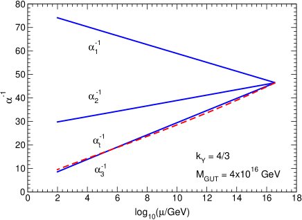
Figure 1: Two-loop evolution of gauge (solid) and top quark Yukawa (dash) couplings, with $k_{Y}=4/3$.

From the trilinear term in the 7D bulk action in Eq. (47) the top quark Yukawa coupling is contained in the term

$$\int d^{7}x\left[\int d^{2}\theta\ g_{7}Q_{3}t^{c}H_{u}+h.c.\right],$$ (9)

where $g_{7}$ is the $SU(7)$ gauge coupling at the compactification scale, which for simplicity, we identify it as $M_{\rm GUT}$. Note that the Higgs superfield $H_{u}$ appears in Eq. (9). We will ignore brane localized gauge kinetic terms, which may be suppressed by taking $VM_{*}\gtrsim O(100)$, where $V$ denotes the volume of the extra dimensions and $M_{*}$ is the cutoff scale [2]. With these caveats we obtain the 4D gauge–top quark Yukawa coupling unification at $M_{\rm GUT}$

$$g_{1}=g_{2}=g_{3}=y_{t}=g_{7}/\sqrt{V},$$ (10)

where $y_{t}$ is the top quark Yukawa coupling.

The top quark coupling to the SM Higgs will pick up an additional factor because the latter arises from the linear combination

$$H\equiv-\cos\beta i\sigma_{2}\,H^{*}_{d}+\sin\beta\,H_{u},$$ (11)

where $\beta$ is the mixing angle and $\sigma_{2}$ is the second Pauli matrix. The effective tree-level top quark Yukawa coupling at $M_{\rm GUT}$ is then given by

$$h_{t}=y_{t}\sin\beta=g_{7}\sin\beta/\sqrt{V}.$$ (12)

Note that the linear combination orthogonal to Eq. (11) is superheavy and does not play a role in low energy phenomenology. Of course, the mass scale of $H$ is fine tuned to be of the order $M_{Z}$.

One possible way to implement the fine tuning is to introduce a brane localized gauge singlet field S with a VEV of order $M_{\rm GUT}$. The superpotential coupling $H_{u}H_{d}S$ induces order $M_{\rm GUT}$ mass terms for the doublets, which combined with order $M_{\rm GUT}$ supersymmetry breaking soft terms, can yield the desired $M_{Z}$ scale for $H$ through fine tuning. Note that the Higgsino mass is of the order $M_{\rm GUT}$, too.

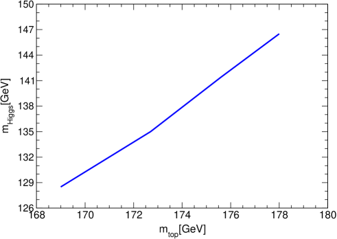
Figure 2: Higgs boson mass $m_{\rm Higgs}$ versus top quark mass $m_{\rm top}$ with gauge–top quark Yukawa coupling unification at $M_{\rm GUT}$.

The quartic Higgs coupling is determined at $M_{\rm GUT}$ by the supersymmetric $D$-term

$$\lambda=\frac{\frac{3}{4}g^{2}_{1}(M_{\rm GUT})+g^{2}_{2}(M_{\rm GUT})}{4}\cos^{2}2\beta.$$ (13)

The renormalization group equation (RGE) for $\lambda$ is given in Eq. (66) in Appendix B. In the numerical calculations we employ two-loop RGEs for the gauge, Yukawa couplings, and Higgs quartic couplings (see Appendix B). There could be threshold corrections to $\lambda(M_{\rm GUT})$ from the supersymmetric spectrum, but since we have not specified a scenario for supersymmetry breaking, we will not consider them here.

Using $\alpha^{-1}_{EM}(M_{Z})=128.91\pm 0.02$  and  $\sin^{2}\theta_{W}(M_{Z})=0.23120\pm 0.00015$ in $\overline{MS}$ scheme [11] and with $k_{Y}=4/3$, we can determine $M_{\rm GUT}$ as well as the unified coupling constant at $M_{\rm GUT}$. Evolving the couplings from $M_{\rm GUT}$ to $M_{Z}$, according to the boundary condition in Eq. (13), we estimate that $\alpha_{3}(m_{Z})\simeq 0.118$, in good agreement with the data [11].

The SM gauge couplings (more precisely $\alpha_{i}^{-1}$) are plotted in Fig. 1, which also displays the coupling $\alpha_{t}^{-1}\equiv 4\pi/y_{t}^{2}$. Knowing $y_{t}$ at low energies allows us to estimate the Higgs mixing angle $\beta$ in Eq. (11) by using the measured value $172.7\pm 2.9$ GeV of the top quark mass [8]. We find $1.3\leq\tan\beta\leq 1.8$, which is inserted in Eq. (13) to fix the Higgs quartic coupling $\lambda(M_{\rm GUT})$. Employing Eq. (66) we can then determine $\lambda$ at low energy.

The Higgs boson mass will be estimated by employing the one–loop effective potential [12]

$$V_{eff}=-m_{h}^{2}H^{\dagger}H+\frac{\lambda}{2}(H^{\dagger}H)^{2}-\frac{3}{16\pi^{2}}h_{t}^{4}(H^{\dagger}H)^{2}\left[\log\frac{h_{t}^{2}(H^{\dagger}H)}{Q^{2}}-\frac{3}{2}\right],$$ (14)

where the coefficient $(-m_{h}^{2})$ of the quadratic term is fine tuned along the line discussed above. The top quark Yukawa coupling to $H$ is $h_{t}=y_{t}\sin\beta$, and the scale $Q$ is chosen to coincide with the Higgs boson mass. In Fig. 2, we plot the Higgs mass versus $m_{\rm top}$. For the presently favored central value $\rm m_{top}=172.7\pm 2.9$ GeV [8], we estimate the Higgs mass to be 135 GeV. It is intriguing that the Higgs mass estimate is somewhat higher then the 126 GeV upper bound on the lightest neutral Higgs boson mass in the MSSM [13].

As far as the remaining charged fermions are concerned, we note that on the 3-brane at the $Z_{6}\times Z_{2}$ fixed point $(z,y)=(0,0)$, the preserved gauge symmetry is $SU(3)_{C}\times SU(2)_{L}\times U(1)_{Y}\times U(1)_{\alpha}\times U(1)_{\beta}$. Thus, on the observable 3-brane at $(z,y)=(0,0)$, we can introduce the first two families of the SM quarks and leptons, the right-handed bottom quark, the $\tau$ lepton doublet, and the right-handed $\tau$ lepton. The $U(1)_{\alpha}\times U(1)_{\beta}$ anomalies can be canceled by assigning suitable charges to the SM quarks and leptons. For example, under $U(1)_{\alpha}\times U(1)_{\beta}$ the charges for the first-family quark doublet and the right-handed up quark can be respectively $(\mathbf{-3},\mathbf{{\sqrt{14}}/2})$ and $(\mathbf{0},\mathbf{-2{\sqrt{14}}})$, while the charges of remaining SM fermions are zero.

4 Unification of Gauge and Bottom Quark Yukawa Couplings

To implement this scenario we make the following choice in Eq. (1):

$$n_{1}~{}=~{}5~{},~{}~{}n_{2}~{}=~{}2~{}{\rm or}~{}3~{}.~{}\,$$ (15)

The identification of $U(1)_{Y}$ differs from the previous Section. The generators of $U(1)_{Y}\times U(1)_{\alpha}\times U(1)_{\beta}$ are defined as follows:

$$T_{U(1)_{Y}}\equiv-{1\over 6}{\rm diag}\left(0,0,0,1,1,-2,0\right)~{}+{{\sqrt{21}}\over{42}}{\rm diag}\left(1,1,1,1,1,1,-6\right),~{}\,$$

$$T_{U(1)_{\alpha}}\equiv{\sqrt{21}}~{}{\rm diag}\left(0,0,0,1,1,-2,0\right)+{\rm diag}\left(1,1,1,1,1,1,-6\right),$$

$$T_{U(1)_{\beta}}\equiv{\rm diag}\left(1,1,1,-1,-1,-1,0\right).$$ (16)

Note that $k_{Y}=4/3$ also in this case.

Chiral Fields	Zero Modes
$\Sigma_{1}$	$Q_{3}$:  $\mathbf{(3,\bar{2})}_{Q12}$
$\Sigma_{2}$	$H_{d}$:  $\mathbf{(1,2)}_{Q23}$;  $H_{u}$:  $\mathbf{(1,\bar{2})}_{Q32}$
$\Sigma_{3}$	$b^{c}$: $\mathbf{(\bar{3},1)}_{Q31}$

Table 2: Zero modes from the chiral multiplets $\Sigma_{1}$, $\Sigma_{2}$ and $\Sigma_{3}$ with gauge and bottom quark Yukawa coupling unification.

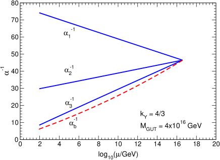
Figure 3: Two-loop evolution of gauge (solid) and bottom quark Yukawa (dash) couplings , with $k_{Y}=4/3$.

The corresponding charges $Qij$ are:

$$Q12=\left(\mathbf{1\over 6},\mathbf{-{\sqrt{21}}},\mathbf{2}\right),~{}~{}~{}~{}~{}Q13=\left(\mathbf{-{1\over 3}},\mathbf{2{\sqrt{21}}},\mathbf{2}\right),$$

$$Q14=\left(\mathbf{{{\sqrt{21}}\over{6}}},\mathbf{7},\mathbf{1}\right),~{}~{}~{}~{}~{}~{}~{}~{}~{}Q34=\left(\mathbf{{2+{\sqrt{21}}}\over 6},\mathbf{7-2{\sqrt{21}}},\mathbf{-1}\right),$$

$$Q24=\left(\mathbf{-{1+{\sqrt{21}}}\over 6},\mathbf{7+{\sqrt{21}}},\mathbf{-1}\right),~{}~{}~{}~{}~{}Q23=\left(\mathbf{-{1\over 2}},\mathbf{3{\sqrt{21}}},\mathbf{0}\right).$$ (17)

In Table 2, we present the zero modes from the chiral multiplets $\Sigma_{1}$, $\Sigma_{2}$ and $\Sigma_{3}$. We identify them with the left-handed doublet ($Q_{3}$), right-handed bottom quark $b^{c}$, and a pair of Higgs doublets $H_{u}$ and $H_{d}$. From the trilinear term in the 7D bulk action in Eq. (47) we obtain the bottom quark Yukawa coupling

$$\int d^{7}x\left[\int d^{2}\theta\ g_{7}Q_{3}b^{c}H_{d}+h.c.\right].~{}\,$$ (18)

Thus, at $M_{\rm GUT}$ we have

$$g_{1}=g_{2}=g_{3}=y_{b}=g_{7}/\sqrt{V},$$ (19)

where $y_{b}$ is the bottom quark Yukawa coupling to $H_{d}$. Then the bottom quark Yukawa coupling to the SM Higgs boson is given by

$$h_{b}=y_{b}\cos\beta=g_{7}\cos\beta/\sqrt{V}~{}.~{}\,$$ (20)

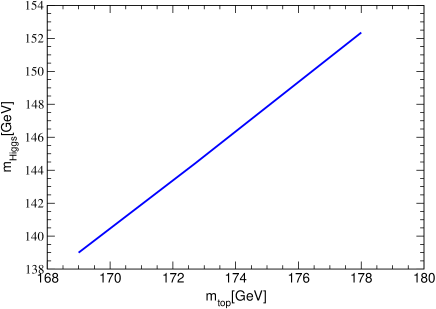
Figure 4: Higgs boson mass versus $m_{top}$ with gauge–bottom quark Yukawa coupling unification at $M_{\rm GUT}$.

Employing the boundary conditions from Eq. (19) and proceeding analogously to the previous (top quark) case, we display the four couplings in Fig.3. Using $m_{b}(m_{b})=4.8$ GeV, we determine the Higgs mass for this scenario to be $144\pm 4$ GeV, as shown in Fig. 4. The mixing angle $\beta$ is given by $\tan\beta\approx 82$, very different from the value ($\tan\beta\approx 1.5$) estimated in the previous (top quark) Section.

5 Gauge and Tau lepton Yukawa Coupling Unification

To realize the gauge–tau lepton Yukawa coupling unification, we set

$$n_{1}~{}=~{}4~{},~{}~{}n_{2}~{}=~{}3;~{}{\rm or}~{}n_{1}~{}=~{}3~{},~{}~{}n_{2}~{}=~{}2~{}.~{}\,$$ (21)

The generators for $U(1)_{Y}\times U(1)_{\alpha}\times U(1)_{\beta}$ are as follows:

$$T_{U(1)_{Y}}\equiv{1\over 2}~{}{\rm diag}\left(0,0,0,0,0,1,-1\right)-~{}{{\sqrt{14}}\over{84}}{\rm diag}\left(4,4,4,-3,-3,-3,-3\right),~{}$$

$$T_{U(1)_{\beta}}\equiv-{{\sqrt{14}}\over{3}}~{}{\rm diag}\left(0,0,0,0,0,1,-1\right)-{1\over 3}~{}{\rm diag}\left(4,4,4,-3,-3,-3,-3\right),$$

$$T_{U(1)_{\alpha}}\equiv{\rm diag}\left(0,0,0,1,1,-1,-1\right).$$ (22)

With ${\rm tr}[T_{U(1)_{Y}}^{2}]=2/3$, we obtain $k_{Y}=4/3$. This insures the gauge coupling unification.

Chiral Fields	Zero Modes
$\Sigma_{1}$	$\tau^{c}$: $\mathbf{(1,1)}_{Q34}$
$\Sigma_{2}$	$H_{d}$:  $\mathbf{(1,2)}_{Q23}$;  $H_{u}$:  $\mathbf{(1,2)}_{Q32}$
$\Sigma_{3}$	$L_{3}$: $\mathbf{(1,2)}_{Q42}$

Table 3: Zero modes from the chiral multiplets $\Sigma_{1}$, $\Sigma_{2}$ and $\Sigma_{3}$ with gauge–tau lepton Yukawa coupling unification.

The $U(1)_{Y}\times U(1)_{\alpha}\times U(1)_{\beta}$ charges $Qij$ are

$$Q12=\left(\mathbf{-{{\sqrt{14}}\over 12}},\mathbf{-{{7}\over 3}},\mathbf{-1}\right),~{}~{}~{}~{}~{}Q13=\left(\mathbf{-{{6+\sqrt{14}}\over 12}},\mathbf{-{{7-\sqrt{14}}\over 3}},\mathbf{1}\right),$$

$$Q23=\left(\mathbf{-{1\over 2}},\mathbf{{\sqrt{14}}\over{3}},\mathbf{2}\right),~{}~{}~{}~{}~{}~{}~{}~{}~{}~{}Q14=\left(\mathbf{{{6-\sqrt{14}}\over 12}},\mathbf{-{{7+\sqrt{14}}\over 3}},\mathbf{1}\right),$$

$$Q24=\left(\mathbf{{1\over 2}},\mathbf{-{{\sqrt{14}}\over{3}}},\mathbf{2}\right),~{}~{}~{}~{}~{}~{}~{}~{}~{}~{}Q34=\left(\mathbf{1},\mathbf{-{{2\sqrt{14}}\over{3}}},\mathbf{0}\right).$$ (23)

In Table 3, we present the zero modes from the chiral multiplets $\Sigma_{1}$, $\Sigma_{2}$ and $\Sigma_{3}$. The zero modes include the third-family left-handed lepton doublet $L_{3}$, one pair of Higgs doublets $H_{u}$ and $H_{d}$, and the right-handed tau lepton $\tau^{c}$. From the trilinear term in the 7D bulk action, we obtain the $\tau$ lepton Yukawa term

$$\int d^{7}x\left[\int d^{2}\theta\ g_{7}L_{3}\tau^{c}H_{d}+h.c.\right].~{}\,$$ (24)

Thus, at $M_{\rm GUT}$, we have

$$g_{1}=g_{2}=g_{3}=y_{\tau}~{},~{}\,$$ (25)

where $y_{\tau}$ is the tau lepton Yukawa coupling.

This case turns out to be quite similar to the gauge–bottom quark Yukawa coupling unification discussed above, with $\tan\beta$ once again large ($\sim$ 50 or so). The Higgs mass is predicted to be close to 144 GeV, with the usual uncertainty of several GeV arising from the lack of a more precise determination of the top quark mass.

6 $SU(8)$ Model

It is possible to construct an $SU(8)$ model with $k_{Y}=4/3$, such that the three SM gauge couplings as well as the two Yukawa couplings are unified at $M_{\rm GUT}$, for example, the top and bottom quark Yukawa couplings. From our previous discussions we note that the unification of the gauge and top quark Yukawa couplings favors a low value of $\tan\beta\sim 1.5$, while the bottom quark (or tau lepton) case requires a much larger value of $\tan\beta\sim 70-85$. Thus, we expect that a scenario in which all five couplings are unified at $M_{\rm GUT}$ will lead to some inconsistency. If we insist that the model correctly reproduces the top quark mass, then the bottom quark mass will not be in agreement with the data without invoking new physics such as higher-dimensional operators. Mindful of this caveat the construction of the $SU(8)$ model proceeds as follows. To break the $SU(8)$ gauge symmetry, we choose the following $8\times 8$ matrix representations for $R_{\Gamma_{T}}$ and $R_{\Gamma_{S}}$

$$R_{\Gamma_{T}} = {\rm diag}\left(+1,+1,+1,\omega^{n_{1}},\omega^{n_{1}},\omega^{n_{1}},\omega^{n_{1}},\omega^{n_{2}}\right),~{}\,$$ (26)

$$R_{\Gamma_{S}} = {\rm diag}\left(+1,+1,+1,+1,+1,-1,-1,-1\right),~{}\,$$ (27)

where $n_{1}$ and $n_{2}$ are positive integers, and $n_{1}\not=n_{2}$. Then, we obtain

$$\{SU(8)/R_{\Gamma_{T}}\}~{}=~{}SU(3)_{C}\times SU(4)\times U(1)\times U(1)^{\prime},~{}\,$$ (28)

$$\{SU(8)/R_{\Gamma_{S}}\}~{}=~{}SU(5)\times SU(3)\times U(1),~{}\,$$ (29)

$$\{SU(8)/\{R_{\Gamma_{T}}\cup R_{\Gamma_{S}}\}\}~{}=~{}SU(3)_{C}\times SU(2)_{L}\times SU(2)_{R}\times U(1)_{X}\times U(1)_{\alpha}\times U(1)_{\beta}.~{}\,$$ (30)

Therefore, we obtain that, for the zero modes, the 7D ${\cal N}=1$ supersymmetric $SU(8)$ gauge symmetry is broken down to the 4-dimensional ${\cal N}=1$ supersymmetric $SU(3)_{C}\times SU(2)_{L}\times SU(2)_{R}\times U(1)_{X}\times U(1)_{\alpha}\times U(1)_{\beta}$ gauge symmetry [3].

We define the generators for the $U(1)_{X}\times U(1)_{\alpha}\times U(1)_{\beta}$ gauge symmetry as follows

$$T_{U(1)_{X}} \equiv {1\over 42}~{}{\rm diag}\left(4,4,4,-3,-3,-3,-3,0\right)+{{\sqrt{15}}\over{84}}~{}T{\rm diag}\left(1,1,1,1,1,1,1,-7\right),~{}\,$$

$$T_{U(1)_{\alpha}} \equiv -{{\sqrt{15}}\over 3}~{}{\rm diag}\left(4,4,4,-3,-3,-3,-3,0\right)+~{}{\rm diag}\left(1,1,1,1,1,1,1,-7\right),~{}\,$$

$$T_{U(1)_{\beta}} \equiv {\rm diag}\left(0,0,0,1,1,-1,-1,0\right).$$ (31)

The $SU(8)$ adjoint representation $\mathbf{63}$ is decomposed under the $SU(3)_{C}\times SU(2)_{L}\times SU(2)_{R}\times U(1)_{X}\times U(1)_{\alpha}\times U(1)_{\beta}$ gauge symmetry as

$$\mathbf{63}=\left(\begin{array}[]{cccc}\mathbf{(8,1,1)}_{Q00}&\mathbf{(3,\bar{2},1)}_{Q12}&\mathbf{(3,1,\bar{2})}_{Q13}&\mathbf{(3,1,1)}_{Q14}\\ \mathbf{(\bar{3},2,1)}_{Q21}&\mathbf{(1,3,1)}_{Q00}&\mathbf{(1,2,\bar{2})}_{Q23}&\mathbf{(1,2,1)}_{Q24}\\ \mathbf{(\bar{3},1,2)}_{Q31}&\mathbf{(1,\bar{2},2)}_{Q32}&\mathbf{(1,1,3)}_{Q00}&\mathbf{(1,1,2)}_{Q34}\\ \mathbf{(\bar{3},1,1)}_{Q41}&\mathbf{(1,\bar{2},1)}_{Q42}&\mathbf{(1,1,\bar{2})}_{Q43}&\mathbf{(1,1,1)}_{Q00}\end{array}\right)+2\mathbf{(1,1,1)}_{Q00}~{},~{}\,$$ (32)

where the $\mathbf{(1,1,1)}_{Q00}$ in the fourth diagonal entry of the matrix and the last term $2\mathbf{(1,1,1)}_{Q00}$ denote the gauge fields for the $U(1)_{X}\times U(1)_{\alpha}\times U(1)_{\beta}$ gauge symmetry. Moreover, the subscripts $Qij$, which are anti-symmetric ($Qij=-Qji$), are the charges under the $U(1)_{X}\times U(1)_{\alpha}\times U(1)_{\beta}$ gauge symmetry. The subscript $Q00~{}=~{}(\mathbf{0},\mathbf{0},\mathbf{0})$, and the other subscripts $Qij$ with $i\not=j$ are

$$Q12=\left(\mathbf{1\over 6},\mathbf{-{{7{\sqrt{15}}}\over{3}}},\mathbf{-1}\right),~{}~{}~{}~{}~{}~{}~{}~{}~{}~{}~{}~{}~{}~{}~{}~{}~{}Q13=\left(\mathbf{1\over 6},\mathbf{-{{7{\sqrt{15}}}\over{3}}},\mathbf{1}\right),$$

$$Q14=\left(\mathbf{{{2+2{\sqrt{15}}}\over{21}}},\mathbf{{{{24-4\sqrt{15}}}\over{3}}},\mathbf{0}\right),~{}~{}~{}Q23=\left(\mathbf{0},\mathbf{0},\mathbf{2}\right),$$

$$Q24=\left(\mathbf{{{{-3+4\sqrt{15}}}\over{42}}},\mathbf{8+\sqrt{15}},\mathbf{1}\right),$$

$$Q34=\left(\mathbf{{{{-3+4\sqrt{15}}}\over{42}}},\mathbf{8+\sqrt{15}},\mathbf{-1}\right).$$ (33)

The $Z_{6}\times Z_{2}$ transformation properties for the decomposed components of $V$, $\Sigma_{1}$, $\Sigma_{2}$, and $\Sigma_{3}$ are still given by Eqs. (56)–(59). And we choose $n_{1}=5$ and $n_{2}=2~{}{\rm or}~{}3$, as in Eq. (6).

In Table 4, we present the zero modes from the chiral multiplets $\Sigma_{1}$, $\Sigma_{2}$ and $\Sigma_{3}$. The zero modes include the left-handed quark doublet $Q_{3}$ for the third family, one pair of bidoublet Higgs fields $\Phi$ and $\overline{\Phi}$, and the right-handed quark doublet $\overline{Q}_{3}$ for the third family. More concretely, the bidoublet Higgs field $\Phi$ contains a pair of Higgs doublets $H_{u}$ and $H_{d}$, and the right-handed quark doublet $\overline{Q}_{3}$ for the third family contains $t^{c}$ and $b^{c}$.

Chiral Fields	Zero Modes
$\Sigma_{1}$	$Q_{3}$:  $\mathbf{(3,\bar{2},1)}_{Q12}$
$\Sigma_{2}$	$\Phi$:  $\mathbf{(1,2,\bar{2})}_{Q23}$;  $\overline{\Phi}$:  $\mathbf{(1,\bar{2},2)}_{Q32}$
$\Sigma_{3}$	$\overline{Q}_{3}$: $\mathbf{(\bar{3},1,2)}_{Q31}$

Table 4: The zero modes of the chiral multiplets $\Sigma_{1}$, $\Sigma_{2}$ and $\Sigma_{3}$ in the 7D $SU(8)$ orbifold model.

From the trilinear term in the 7D bulk action, we obtain the quark Yukawa term

$$\int d^{7}x\left[\int d^{2}\theta\ g_{8}Q_{3}\overline{Q}_{3}\Phi+h.c.\right],~{}\,$$ (34)

where $g_{8}$ is the $SU(8)$ gauge coupling at $M_{\rm GUT}$.

In order to break the $SU(2)_{R}\times U(1)_{X}$ gauge symmetry down to the $U(1)_{Y}$ gauge symmetry, we introduce one pair of Higgs doublets $H_{1}$ and $H_{2}$ with quantum numbers $\mathbf{(2,-1/2)}$ and $\mathbf{(2,+1/2)}$ under the $SU(2)_{R}\times U(1)_{X}$ gauge symmetry on the observable 3-brane, and assign the following VEVs:

$$\langle H_{1}\rangle~{}=~{}\left(\begin{array}[]{c}v_{X}\\ 0\end{array}\right),~{}~{}~{}~{}\langle H_{2}\rangle~{}=~{}\left(\begin{array}[]{c}0\\ v_{X}\end{array}\right).~{}\,$$ (39)

The $U(1)_{Y}$ generator in $SU(8)$ is given by

$$T_{U(1)_{Y}} \equiv {\rm diag}\left({{8+{\sqrt{15}}}\over{84}},{{8+{\sqrt{15}}}\over{84}},{{8+{\sqrt{15}}}\over{84}},{{-6+{\sqrt{15}}}\over{84}},{{-6+{\sqrt{15}}}\over{84}},\right.$$ (40)

$$\left.{{-48+{\sqrt{15}}}\over{84}},{{36+{\sqrt{15}}}\over{84}},-{{\sqrt{15}}\over{12}}\right).~{}\,$$

Because ${\rm tr}[T_{U(1)_{Y}}^{2}]=2/3$, we obtain $k_{Y}=4/3$.

With $SU(2)_{R}\times U(1)_{X}$ broken to $U(1)_{Y}$, the third-family quark Yukawa couplings are

$$\int d^{7}x\left[\int d^{2}\theta\ g_{8}\left(Q_{3}t^{c}H_{u}+Q_{3}b^{c}H_{d}\right)+h.c.\right].~{}\,$$ (41)

Thus, at the $M_{\rm GUT}$ scale, we have

$$g_{1}=g_{2}=g_{3}=y_{t}=y_{b}\,.~{}\,$$ (42)

Employing the boundary conditions in Eq. (42) and making sure that the top quark mass is reproduced correctly, we expect the Higgs mass to be around $135\pm 6$ GeV. The bottom quark mass turns out to be a factor two larger than its measured value and, as mentioned earlier, suitable non-renormalizable operators must be introduced to rectify this. These additional operators are not expected to significantly change the Higgs mass prediction.

7 Conclusions

We have considered a class of 7D orbifold GUTs with ${\cal N}=1$ supersymmetry in which the mass of the SM Higgs boson can be reliably predicted. Depending on the details of the models the mass is around 135 or 144 GeV, which is comfortably above the upper bound on the mass of the lightest Higgs boson in the MSSM. The discovery of the Higgs boson in the above mass range would be a boost for the framework considered in this paper, namely that the unification of the SM gauge couplings can be realized without low-energy supersymmetry by invoking a non-canonical normalization of $U(1)_{Y}$.

Appendix A: Seven-Dimensional Orbifold Models

We consider a 7D space-time $M^{4}\times T^{2}/Z_{6}\times S^{1}/Z_{2}$ with coordinates $x^{\mu}$, ($\mu=0,1,2,3$), $x^{5}$, $x^{6}$ and $x^{7}$. The torus $T^{2}$ is homeomorphic to $S^{1}\times S^{1}$ and the radii of the circles along the $x^{5}$, $x^{6}$ and $x^{7}$ directions are $R_{1}$, $R_{2}$, and $R^{\prime}$, respectively. We define the complex coordinate $z$ for $T^{2}$ and the real coordinate $y$ for $S^{1}$,

$$z\equiv{1\over 2}\left(x^{5}+ix^{6}\right),~{}~{}~{}~{}~{}~{}~{}~{}~{}~{}y\equiv x^{7}.$$ (43)

The torus $T^{2}$ can be defined by $C^{1}$ modulo the equivalent classes:

$$z\sim z+\pi R_{1},~{}~{}~{}~{}~{}~{}~{}~{}~{}~{}~{}z\sim z+\pi R_{2}e^{{\rm i}\theta}.$$ (44)

To obtain the orbifold $T^{2}/Z_{6}$, we require that $R_{1}=R_{2}\equiv R$ and $\theta=\pi/3$. Then $T^{2}/Z_{6}$ is obtained from $T^{2}$ by moduloing the equivalent class

$$\Gamma_{T}:~{}~{}~{}z\sim\omega z,~{}\,$$ (45)

where $\omega=e^{{\rm i}\pi/3}$. There is one $Z_{6}$ fixed point $z=0$, two $Z_{3}$ fixed points: $z=\pi Re^{{\rm i}\pi/6}/{\sqrt{3}}$ and $z=2\pi Re^{{\rm i}\pi/6}/{\sqrt{3}}$, and three $Z_{2}$ fixed points: $z=\sqrt{3}\pi Re^{{\rm i}\pi/6}/2$, $z=\pi R/2$ and $z=\pi Re^{{\rm i}\pi/3}/2$. The orbifold $S^{1}/Z_{2}$ is obtained from $S^{1}$ by moduloing the equivalent class

$$\Gamma_{S}:~{}~{}~{}y\sim-y~{}.~{}\,$$ (46)

There are two fixed points: $y=0$ and $y=\pi R^{\prime}$. The ${\cal N}=1$ supersymmetry in 7D has 16 supercharges corresponding to ${\cal N}=4$ supersymmetry in 4D, and only the gauge multiplet can be introduced in the bulk. This multiplet can be decomposed under 4D ${\cal N}=1$ supersymmetry into a gauge vector multiplet $V$ and three chiral multiplets $\Sigma_{1}$, $\Sigma_{2}$, and $\Sigma_{3}$ in the adjoint representation, where the fifth and sixth components of the gauge field, $A_{5}$ and $A_{6}$, are contained in the lowest component of $\Sigma_{1}$, and the seventh component of the gauge field $A_{7}$ is contained in the lowest component of $\Sigma_{2}$.

We express the bulk action in the Wess–Zumino gauge and 4D ${\cal N}=1$ supersymmetry notation  [9]

$${\cal S} = \int d^{7}x\Biggl{\{}{\rm Tr}\Biggl{[}\int d^{2}\theta\left(\frac{1}{4kg^{2}}{\cal W}^{\alpha}{\cal W}_{\alpha}+\frac{1}{kg^{2}}\left(\Sigma_{3}\partial_{z}\Sigma_{2}+\Sigma_{1}\partial_{y}\Sigma_{3}-\frac{1}{\sqrt{2}}\Sigma_{1}[\Sigma_{2},\Sigma_{3}]\right)\right)$$ (47)

$$+h.c.\Biggr{]}+\int d^{4}\theta\frac{1}{kg^{2}}{\rm Tr}\Biggl{[}(\sqrt{2}\partial_{z}^{\dagger}+\Sigma_{1}^{\dagger})e^{-V}(-\sqrt{2}\partial_{z}+\Sigma_{1})e^{V}+\partial_{z}^{\dagger}e^{-V}\partial_{z}e^{V}$$

$$+(\sqrt{2}\partial_{y}+\Sigma_{2}^{\dagger})e^{-V}(-\sqrt{2}\partial_{y}+\Sigma_{2})e^{V}+\partial_{y}e^{-V}\partial_{y}e^{V}+{\Sigma_{3}}^{\dagger}e^{-V}\Sigma_{3}e^{V}\Biggr{]}\Biggr{\}},~{}\,$$

where $k$ is the normalization of the group generator, and  ${\cal W_{\alpha}}$  denotes the gauge field strength. From the above action, we obtain the transformations of the vector multiplet:

$$V(x^{\mu},~{}\omega z,~{}\omega^{-1}{\bar{z}},~{}y) = R_{\Gamma_{T}}V(x^{\mu},~{}z,~{}{\bar{z}},~{}y)R_{\Gamma_{T}}^{-1}~{},~{}\,$$ (48)

$$\Sigma_{1}(x^{\mu},~{}\omega z,~{}\omega^{-1}{\bar{z}},~{}y) = \omega^{-1}R_{\Gamma_{T}}\Sigma_{1}(x^{\mu},~{}z,~{}{\bar{z}},~{}y)R_{\Gamma_{T}}^{-1}~{},~{}\,$$ (49)

$$\Sigma_{2}(x^{\mu},~{}\omega z,~{}\omega^{-1}{\bar{z}},~{}y) = R_{\Gamma_{T}}\Sigma_{2}(x^{\mu},~{}z,~{}{\bar{z}},~{}y)R_{\Gamma_{T}}^{-1}~{},~{}\,$$ (50)

$$\Sigma_{3}(x^{\mu},~{}\omega z,~{}\omega^{-1}{\bar{z}},~{}y) = \omega R_{\Gamma_{T}}\Sigma_{3}(x^{\mu},~{}z,~{}{\bar{z}},~{}y)R_{\Gamma_{T}}^{-1}~{},~{}\,$$ (51)

$$V(x^{\mu},~{}z,~{}{\bar{z}},~{}-y) = R_{\Gamma_{S}}V(x^{\mu},~{}z,~{}{\bar{z}},~{}y)R_{\Gamma_{S}}^{-1}~{},~{}\,$$ (52)

$$\Sigma_{1}(x^{\mu},~{}z,~{}{\bar{z}},~{}-y) = R_{\Gamma_{S}}\Sigma_{1}(x^{\mu},~{}z,~{}{\bar{z}},~{}y)R_{\Gamma_{S}}^{-1}~{},~{}\,$$ (53)

$$\Sigma_{2}(x^{\mu},~{}z,~{}{\bar{z}},~{}-y) = -R_{\Gamma_{S}}\Sigma_{2}(x^{\mu},~{}z,~{}{\bar{z}},~{}y)R_{\Gamma_{S}}^{-1}~{},~{}\,$$ (54)

$$\Sigma_{3}(x^{\mu},~{}z,~{}{\bar{z}},~{}-y) = -R_{\Gamma_{S}}\Sigma_{3}(x^{\mu},~{}z,~{}{\bar{z}},~{}y)R_{\Gamma_{S}}^{-1}~{},~{}\,$$ (55)

where we introduce non-trivial transformation $R_{\Gamma_{T}}$ and $R_{\Gamma_{S}}$ to break the bulk gauge group $G$.

The $Z_{6}\times Z_{2}$ transformation properties for the decomposed components of $V$, $\Sigma_{1}$, $\Sigma_{2}$, and $\Sigma_{3}$ in our $SU(7)$ and $SU(8)$ models are given by

$$V:\left(\begin{array}[]{cccc}(1,+)&(\omega^{-n_{1}},+)&(\omega^{-n_{1}},-)&(\omega^{-n_{2}},-)\\ (\omega^{n_{1}},+)&(1,+)&(1,-)&(\omega^{n_{1}-n_{2}},-)\\ (\omega^{n_{1}},-)&(1,-)&(1,+)&(\omega^{n_{1}-n_{2}},+)\\ (\omega^{n_{2}},-)&(\omega^{n_{2}-n_{1}},-)&(\omega^{n_{2}-n_{1}},+)&(1,+)\end{array}\right)+(1,+)~{},~{}\,$$ (56)

$$\Sigma_{1}:\left(\begin{array}[]{cccc}(\omega^{-1},+)&(\omega^{-n_{1}-1},+)&(\omega^{-n_{1}-1},-)&(\omega^{-n_{2}-1},-)\\ (\omega^{n_{1}-1},+)&(\omega^{-1},+)&(\omega^{-1},-)&(\omega^{n_{1}-n_{2}-1},-)\\ (\omega^{n_{1}-1},-)&(\omega^{-1},-)&(\omega^{-1},+)&(\omega^{n_{1}-n_{2}-1},+)\\ (\omega^{n_{2}-1},-)&(\omega^{n_{2}-n_{1}-1},-)&(\omega^{n_{2}-n_{1}-1},+)&(\omega^{-1},+)\end{array}\right)+(\omega^{-1},+)~{},~{}\,$$ (57)

$$\Sigma_{2}:\left(\begin{array}[]{ccccc}(1,-)&(\omega^{-n_{1}},-)&(\omega^{-n_{1}},+)&(\omega^{-n_{2}},+)\\ (\omega^{n_{1}},-)&(1,-)&(1,+)&(\omega^{n_{1}-n_{2}},+)\\ (\omega^{n_{1}},+)&(1,+)&(1,-)&(\omega^{n_{1}-n_{2}},-)\\ (\omega^{n_{2}},+)&(\omega^{n_{2}-n_{1}},+)&(\omega^{n_{2}-n_{1}},-)&(1,-)\end{array}\right)+(1,-)~{},~{}\,$$ (58)

$$\Sigma_{3}:\left(\begin{array}[]{ccccc}(\omega,-)&(\omega^{-n_{1}+1},-)&(\omega^{-n_{1}+1},+)&(\omega^{-n_{2}+1},+)\\ (\omega^{n_{1}+1},-)&(\omega,-)&(\omega,+)&(\omega^{n_{1}-n_{2}+1},+)\\ (\omega^{n_{1}+1},+)&(\omega,+)&(\omega,-)&(\omega^{n_{1}-n_{2}+1},-)\\ (\omega^{n_{2}+1},+)&(\omega^{n_{2}-n_{1}+1},+)&(\omega^{n_{2}-n_{1}+1},-)&(\omega,-)\end{array}\right)+(\omega,-)~{},~{}\,$$ (59)

where the zero modes transform as $(1,+)$.

From Eqs. (56)–(59), we find that the 7D ${\cal N}=1$ supersymmetric gauge symmetry $SU(7)$ and $SU(8)$ is broken down to 4D ${\cal N}=1$ supersymmetric gauge symmetry $SU(3)_{C}\times SU(2)_{L}\times U(1)_{Y}\times U(1)_{\alpha}\times U(1)_{\beta}$ and $SU(3)_{C}\times SU(2)_{L}\times SU(2)_{R}\times U(1)_{X}\times U(1)_{\alpha}\times U(1)_{\beta}$, respectively [3]. In addition, there are zero modes from the chiral multiplets $\Sigma_{1}$, $\Sigma_{2}$ and $\Sigma_{3}$ which play an important role in gauge–Higgs–Yukawa unification.

Appendix B: Renormalization Group Equations

The two-loop RGEs for the gauge couplings are [14]

$$(4\pi)^{2}\frac{d}{dt}~{}g_{i}=g_{i}^{3}b_{i}+\frac{g_{i}^{3}}{(4\pi)^{2}}\left[\sum_{j=1}^{3}B_{ij}g_{j}^{2}-\sum_{\alpha=u,d,e}d_{i}^{\alpha}{\rm Tr}\left(h_{\alpha}^{\dagger}h_{\alpha}\right)\right],~{}\,$$ (60)

The beta-function coefficients for $SU(3)_{c}\times SU(2)_{L}\times U(1)_{Y}$ , with non-canonical $k_{Y}=\frac{4}{3}$ normalization for $U(1)_{Y}$, are

$$b_{i}=\left(-7,\,-\frac{19}{6},\,\frac{41}{8}\right),~{}~{}~{}~{}\,\,\,\,b_{ij}=\left(\begin{array}[]{ccc}-26&\frac{9}{2}&\frac{11}{8}\\ 12&\frac{35}{6}&\frac{1}{2}\\ 11&\frac{27}{4}&\frac{199}{32}\end{array}\right),$$ (61)

$$d^{u}=\left(2,\frac{3}{2},\frac{17}{8}\right),~{}~{}~{}~{}~{}~{}d^{d}=\left(2,\frac{3}{2},\frac{5}{8}\right),~{}~{}~{}~{}~{}~{}d^{e}=\left(0,\frac{1}{2},\frac{15}{8}\right).~{}\,$$ (62)

The two-loop RGE for the Yukawa couplings and the Higgs quartic coupling $\lambda$, with non-canonical $k_{Y}=\frac{4}{3}$ normalization for $U(1)_{Y}$, are

$$\frac{d}{dt}~{}h_{u} = \frac{h_{u}}{16\pi^{2}}\left[-\sum_{i=1}^{3}c_{i}^{u}g_{i}^{2}+\frac{3}{2}h_{u}^{2}-\frac{3}{2}h_{d}^{2}+\Delta_{2}\right]$$ (63)

$$+ \frac{h_{u}}{(16\pi^{2})^{2}}\left[\frac{1187}{384}g^{4}_{1}-\frac{23}{4}g^{4}_{2}-108g^{4}_{3}-\frac{9}{16}g^{2}_{1}g^{2}_{2}+\frac{19}{12}g^{2}_{1}g^{2}_{3}+9g^{2}_{2}g^{2}_{3}+\frac{5}{2}\Delta_{3}\right.$$

$$+ \left.\left[\frac{223}{64}g^{2}_{1}+\frac{135}{16}g^{2}_{2}+16g_{3}^{2}\right]h_{u}^{2}-\left[\frac{43}{64}g^{2}_{1}-\frac{9}{16}g^{2}_{2}+16g_{3}^{2}\right]h_{d}^{2}-6\lambda h_{u}^{2}\right.$$

$$+ \left.\frac{3}{2}h_{u}^{2}-\frac{5}{4}h_{u}^{2}h_{d}^{2}+\frac{11}{4}h_{d}^{4}+\left[\frac{5}{4}h_{d}^{2}-\frac{9}{4}h_{u}^{2}\right]\Delta_{2}-\Delta_{5}+\frac{3}{2}\lambda^{2}\right]~{},~{}$$

$$\frac{d}{dt}~{}h_{d} = \frac{h_{d}}{16\pi^{2}}\left[-\sum_{i=1}^{3}c_{i}^{d}g_{i}^{2}-\frac{3}{2}h_{u}^{\dagger}h_{u}+\frac{3}{2}h_{d}^{\dagger}h_{d}+\Delta_{2}\right]$$ (64)

$$+ \frac{h_{d}}{(16\pi^{2})^{2}}\left[-\frac{127}{384}g_{1}^{2}-\frac{23}{4}g_{2}^{2}-108g_{3}^{2}-\frac{27}{16}g_{1}^{2}g_{2}^{2}+\frac{31}{12}g_{1}^{2}g_{3}^{2}+9g_{2}^{2}g_{3}^{2}\right.$$

$$- \left.\left[\frac{79}{64}g_{2}^{2}-\frac{9}{16}g_{2}^{2}+16g_{3}^{2}\right]h_{u}^{2}+\left[\frac{187}{64}g_{2}^{2}+\frac{135}{16}g_{2}^{2}+16g_{3}^{2}\right]h_{d}^{2}+\frac{5}{2}\Delta_{3}\right.$$

$$- \left.6\lambda h_{d}^{2}+\frac{3}{2}h_{d}^{4}-\frac{5}{4}h_{d}^{2}h_{u}^{2}+\frac{11}{4}h_{u}^{4}+\left[\frac{5}{4}h_{u}^{2}-\frac{9}{4}h_{d}^{2}\right]\Delta_{2}+\Delta_{5}+\frac{3}{2}\lambda^{2}\right],$$

$$\frac{d}{dt}~{}h_{e} = \frac{h_{e}}{16\pi^{2}}\left[-\sum_{i=1}^{3}c_{i}^{e}g_{i}^{2}+\frac{3}{2}h_{e}^{\dagger}h_{e}+\Delta_{2}\right]$$ (65)

$$+ \frac{h_{d}}{(16\pi^{2})^{2}}\left[\frac{1371}{128}g_{1}^{4}+\frac{23}{4}g_{2}^{4}+\frac{27}{16}g_{1}^{2}g_{2}^{2}+\left[\frac{387}{64}g_{1}^{2}+\frac{135}{16}g_{2}^{2}\right]h_{e}^{2}\right.$$

$$+ \left.\frac{5}{2}\Delta_{3}-6\lambda_{e}^{2}+\frac{3}{2}h_{e}^{4}+\frac{9}{4}\Delta_{2}h_{e}^{2}+\Delta_{5}+\frac{3}{2}\lambda^{2}\right],$$

$$\frac{d}{dt}~{}\lambda = \frac{1}{16\pi^{2}}\left[12\lambda^{2}-\left[\frac{9}{4}g_{1}^{2}+9g_{2}^{2}\right]\lambda+{9\over 4}\left[\frac{1}{3}\frac{3}{16}g_{1}^{4}+\frac{1}{2}g_{1}^{2}g_{2}^{2}+g_{2}^{4}\right]4\Delta_{2}\lambda-4\Delta_{4}\right]$$ (66)

$$+ \frac{1}{(16\pi^{2})^{2}}\left[\left[\frac{27}{2}g_{1}^{2}+54g_{2}^{2}\right]\lambda^{2}+\left[\frac{73}{8}g_{2}^{4}+\frac{117}{16}g_{1}^{2}g_{2}^{2}+\frac{1887}{128}g_{2}^{4}\right]\lambda+\frac{305}{8}g_{2}^{6}\right.$$

$$- \left.\frac{867}{96}g_{1}^{2}g_{2}^{4}-\frac{3411}{512}g_{1}^{6}+64g_{3}^{2}\left[h_{u}^{4}+h_{d}^{4}\right]-\frac{1}{2}g_{1}^{2}\left[2h_{u}^{4}-h_{d}^{4}+3h_{e}^{4}\right]\right.$$

$$+ \left.\frac{3}{4}g_{1}^{2}\left[\left[21g_{2}^{2}-\frac{57}{8}g_{1}^{2}\right]h_{u}^{2}+\left[\frac{15}{8}g_{1}^{2}+9g_{2}^{2}\right]h_{d}^{2}+\left[11g_{2}-\frac{75}{8}g_{1}^{2}\right]h_{e}^{2}\right]\right.$$

$$- \left.\frac{3}{2}g_{2}^{4}\Delta_{2}-\lambda\Delta_{4}+24\lambda^{2}\Delta_{2}+10\lambda\Delta_{3}-42\lambda h_{u}^{2}h_{d}^{2}+20\left[3h_{u}^{6}+3h_{d}^{6}+h_{e}^{6}\right]\right.$$

$$+ \left.12\left[h_{u}^{4}h_{d}^{2}+h_{u}^{2}h_{d}^{4}\right]-78\lambda^{3}-\frac{1677}{128}g_{1}^{4}g_{2}^{2}\right],$$

where

$$c^{u}_{i}=\left(8,\frac{9}{4},\frac{17}{16}\right),~{}~{}~{}~{}~{}~{}~{}c^{d}_{i}=\left(8,\frac{9}{4},\frac{5}{16}\right),~{}~{}~{}~{}~{}~{}~{}c^{e}_{i}=\left(0,\frac{9}{4},\frac{45}{16}\right),~{}$$ (67)

$$\Delta_{2}=3\,h_{u}^{2}+3\,h_{d}^{2}+h_{e}^{2}\,,$$ (68)

$$\Delta_{3}=\sum c_{i}^{u}g_{i}h_{u}^{2}+\sum c_{i}^{d}g_{i}h_{d}^{2}+\frac{1}{3}\sum c_{i}^{e}g_{i}^{2}h_{e}\,,$$ (69)

$$\Delta_{4}=3\,h_{u}^{4}+3\,h_{d}^{4}+h_{e}^{4}\,,$$ (70)

$$\Delta_{5}=\frac{9}{4}\left[3\,h_{u}^{2}+3\,h_{d}^{2}+h_{e}^{2}-\frac{2}{3}h_{u}^{2}h_{d}^{2}\right].$$ (71)

References

- [1] V. Barger, J. Jiang, P. Langacker and T. Li, Phys. Lett. B 624, 233 (2005); Nucl. Phys. B 726, 149 (2005).
- [2] see, for example, Y. Kawamura, Prog. Theor. Phys. 103, 613 (2000); 105, 999 (2001); G. Altarelli and F. Feruglio, Phys. Lett. B 511, 257 (2001); A. B. Kobakhidze, Phys. Lett. B 514, 131 (2001); L. Hall and Y. Nomura, Phys. Rev. D 64, 055003 (2001); A. Hebecker and J. March-Russell, Nucl. Phys. B 613, 3 (2001).
- [3] T. Li, Phys. Lett. B 520, 377 (2001); Nucl. Phys. B 619, 75 (2001); Nucl. Phys. B 633, 83 (2002).
- [4] J. Scherk and J. H. Schwarz, Phys. Lett. B 82, 60 (1979).
- [5] R. Bousso and J. Polchinski, JHEP 0006, 006 (2000); S. B. Giddings, S. Kachru and J. Polchinski, Phys. Rev. D 66, 106006 (2002); S. Kachru, R. Kallosh, A. Linde and S. P. Trivedi, Phys. Rev. D 68, 046005 (2003); L. Susskind, arXiv:hep-th/0302219; F. Denef and M. R. Douglas, JHEP 0405, 072 (2004).
- [6] see, for example, I. Antoniadis, K. Benakli and M. Quiros, New J. Phys. 3, 20 (2001); G. R. Dvali, S. Randjbar-Daemi and R. Tabbash, Phys. Rev. D 65, 064021 (2002); G. Burdman and Y. Nomura, Nucl. Phys. B 656 (2003) 3; N. Haba and Y. Shimizu, Phys. Rev. D 67 (2003) 095001; K. w. Choi, N. y. Haba, K. S. Jeong, K. i. Okumura, Y. Shimizu and M. Yamaguchi, JHEP 0402, 037 (2004); Q. Shafi and Z. Tavartkiladze, Phys. Rev. D 66, 115002 (2002), I. Gogoladze, Y. Mimura, S. Nandi, Phys. Lett. B 560 (2003) 204; C. A. Scrucca, M. Serone, L. Silvestrini and A. Wulzer, JHEP 0402, 049 (2004); G. Panico, M. Serone and A. Wulzer, arXiv:hep-ph/0510373. A. Aranda and J. L. Diaz-Cruz, arXiv:hep-ph/0510138. N. Haba, S. Matsumoto, N. Okada and T. Yamashita, arXiv:hep-ph/0511046. Y. Hosotani, S. Noda, Y. Sakamura and S. Shimasaki, arXiv:hep-ph/0601241.
- [7] I. Gogoladze, Y. Mimura and S. Nandi, Phys. Lett. B 562, 307 (2003); Phys. Rev. Lett. 91, 141801 (2003); Phys. Rev. D 69, 075006 (2004); I. Gogoladze, Y. Mimura, S. Nandi and K. Tobe, Phys. Lett. B 575, 66 (2003); I. Gogoladze, T. Li, Y. Mimura and S. Nandi, Phys. Lett. B 622, 320 (2005); Phys. Rev. D 72, 055006 (2005).
- [8] [CDF Collaboration], arXiv:hep-ex/0507091.
- [9] N. Marcus, A. Sagnotti and W. Siegel, Nucl. Phys. B 224, 159 (1983); N. Arkani-Hamed, T. Gregoire and J. Wacker, JHEP 0203, 055 (2002).
- [10] C. D. Froggatt and H. B. Nielsen, Nucl. Phys. B147 (1979) 277.
- [11] S. Eidelman et al. [Particle Data Group Collab.], Phys. Lett. B 592, (2004) 1.
- [12] G. Altarelli and G. Isidori, Phys. Lett. B 337, 141 (1994); J. A. Casas, J. R. Espinosa and M. Quiros, Phys. Lett. B 342, 171 (1995); M. A. Diaz, T. A. ter Veldhuis and T. J. Weiler, Phys. Rev. D 54, 5855 (1996).
- [13] See for example, M. Carena, H. E. Haber, Prog. Part. Nucl. Phys. 50, (2003) 63 and references therein.
- [14] M. E. Machacek and M. T. Vaughn, Nucl. Phys. B 222, 83 (1983); Nucl. Phys. B 236, 221 (1984); Nucl. Phys. B 249, 70 (1985); C. Ford, I. Jack and D. R. T. Jones, Nucl. Phys. B 387, 373 (1992) [Erratum-ibid. B 504, 551 (1997)]; M. x. Luo and Y. Xiao, Phys. Rev. Lett. 90, 011601 (2003).