$K\to 3\pi$ Final State Interactions at NLO in CHPT and Cabibbo’s Proposal to Measure $a_{0}-a_{2}$

Elvira Gámiz^a), Joaquim Prades^b) and Ignazio Scimemi^c)

^a) Department of Physics and Astronomy, The University of Glasgow

Glasgow G12 8QQ, United Kingdom.

^b) CAFPE and Departamento de Física Teórica y del Cosmos, Universidad de Granada,

Campus de Fuente Nueva, E-18002 Granada, Spain.

^c) Departament de Física Teòrica, IFIC, CSIC-Universitat de València,

Apt. de Correus 22085, E-46071 València, Spain.

We present the analytical results for the $K\to 3\pi$ final state interaction phases at next-to-leading order (NLO) in CHPT. We also study the recent Cabibbo’s proposal to measure the $\pi\pi$ scattering lengths combination $a_{0}-a_{2}$ from the cusp effect in the $\pi^{0}\pi^{0}$ energy spectrum at threshold for $K^{+}\to\pi^{0}\pi^{0}\pi^{+}$ and $K_{L}\to\pi^{0}\pi^{0}\pi^{0}$, and give the relevant formulas to describe it at NLO. We estimate the theoretical uncertainty of the $a_{0}-a_{2}$ determination at NLO in our approach and obtain that it is not smaller than 5 % if added quadratically and 7 % if linearly for $K^{+}\to\pi^{0}\pi^{0}\pi^{+}$. One gets similar theoretical uncertainties if the neutral $K_{L}\to\pi^{0}\pi^{0}\pi^{0}$ decay data below threshold are used instead. For this decay, there are very large theoretical uncertainties above threshold due to cancellations and data above threshold cannot be used to get the scattering lengths. We do not include isospin corrections apart of two-pion phase space factors which are physical. We compare our results for the cusp effect with Cabibbo and Isidori’s ones.

1 Introduction

Final state interaction (FSI) phases at next-to-leading order (NLO) in Chiral Perturbation Theory (CHPT) [3, 4] are needed to obtain the charged CP-violating asymmetries at NLO [5, 6, 7]. The dominant contribution to these $K^{+}\to 3\pi$ FSI at NLO are from two-pion cuts for topology A in Figure 1. They were calculated analytically in [5].

Though to get the full $K\to 3\pi$ amplitudes at order $p^{6}$ implies a two-loop calculation, one can get the FSI phases at NLO using the optical theorem within CHPT with the advantage that one just needs to know $\pi\pi$ scattering and $K\to 3\pi$ both at ${\cal O}(p^{4})$. Notice that NLO in the dispersive part of the amplitude means one-loop and ${\cal O}(p^{4})$ in CHPT while NLO in the absorptive part of the amplitude means two-loops and ${\cal O}(p^{6})$ in CHPT.

In [5] we took the $\pi\pi$ scattering results from [8] and calculated the amplitudes $K\to 3\pi$ at NLO in the isospin limit. We agreed with the NLO $K\to 3\pi$ results recently published in [9]. These were previously calculated in [10] and used in [11], but unfortunately the analytical full results were not available there. Now, there is also available the full one-loop $K\to 3\pi$ amplitudes including isospin breaking effects from quark masses and electromagnetic interactions [12, 13].

In the meantime, we discovered some small errata in the published formulas in [5] which were corrected in [6]. We correct here another erratum in Eqs. (6.6), (6.7) and (6.9) in [5] where we wrote $\mathbb{R}$ instead of $\widetilde{\mathbb{R}}$. See Section 3 in the present work for the correction. In addition, matrix elements 21 and 22 in Eqs. (6.7) and (6.9) in [5] were interchanged. None of these errata affects the results for the CP-violating asymmetries nor the conclusions given in [5, 6, 7].

The details of the use of the optical theorem to calculate the two-pion cut contributions from topology A in Figure 1 were given in Appendix E of the first reference in [5] –solid circle and solid square vertices include both tree and one-loop level. We don’t repeat these details now.

Notice that diagrams B and C are included in topology A when one takes one of the solid vertices at tree level and the other one at one-loop. We plot explicitly diagrams B and C since we will refer to them later.

In the first part of this work, we complete the calculation of all $K\to 3\pi$ FSI phases at NLO in CHPT by evaluating the three-pion cuts in topologies C, D and E in Figure 1 for $K^{+}\to 3\pi$. We also provide with the neutral kaon $K_{L,S}\to 3\pi$ final state interactions at ${\cal O}(p^{6})$ including both two- and three-pion cut contributions. Thus, we give the full $K\to 3\pi$ FSI phases at NLO in CHPT in the isospin limit for all $K\to 3\pi$ decays.

The study of FSI in $K\to 3\pi$ at NLO also became of relevance after the proposal by Cabibbo [14] to measure the combination $a_{0}-a_{2}$ of $\pi\pi$ scattering lengths using the cusp effect in the $\pi^{0}\pi^{0}$ spectrum at threshold in $K^{+}\to\pi^{0}\pi^{0}\pi^{+}$ and $K_{L}\to\pi^{0}\pi^{0}\pi^{0}$ decay rates. Within this proposal, it has been recently presented in [16] the effects of FSI at NLO using formulas dictated by unitarity and analyticity approximated at second order in the $\pi\pi$ scattering lengths, $a_{i}\sim 0.2$. The error was therefore canonically assumed to be of order of $a_{i}^{2}$, i.e., $5\%$. There, they used a second order polynomial in the relevant final two-pion invariant energy $s_{3}$ fitted to data to describe the $K\to 3\pi$ vertex that enters in the formulas of the cusp effect. It is of interest to check this canonical error and provide a complementary analysis of the theoretical uncertainty.

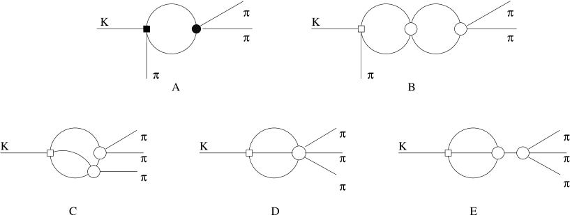
Figure 1: Topologies contributing to FSI in $K\to 3\pi$ decays at LO and NLO. Squares are weak vertices and circles are the strong ones. In topology A, solid circle and solid square vertices include both tree- and one-loop level. See text for more details.

In this work, we use our NLO in CHPT results for the real part of $K\to 3\pi$ fitted to data to describe the $K\to 3\pi$ vertex that enters in formulas of the cusp effect. Notice that we do not want to predict the real part of $K\to 3\pi$ in CHPT at any order but to have the best possible description fitted to data. We treat $\pi\pi$ scattering near threshold as in Cabibbo’s original proposal. The advantage of using CHPT formulas for the fit to data of the real part of $K\to 3\pi$ is that it contains the correct singularity structure at NLO in CHPT which can be systematically improved by going at higher orders. On the other hand, this proposal is not (and cannot be) a CHPT calculation.

Contributions from next-to-next-to-leading order (NNLO) SU(3) CHPT in the isospin limit are expected typically to be around $(3\sim 5)\%$, so that our NLO results are just a first step in order to reduce the theoretical error on the determination of the combination $a_{0}-a_{2}$ to the few per cent level. At NNLO, one can follow a procedure analogous to the one we use here to get a more accurate measurement of $a_{0}-a_{2}$ and check the assumed NNLO uncertainty. At that point, and in order to reach the few per cent level in the theoretical uncertainty, it will be necessary to include full isospin breaking effects at NLO too. These are also expected to be of a few per cent as was found for $K\to 3\pi$ in [12, 13].

In Sections 2 and 3 we introduce the needed notation in the description of $K\to 3\pi$ in CHPT and the $K^{0}\to 3\pi$ final state interaction phases at NLO, respectively. This completes the $K^{+}\to 3\pi$ FSI phases already presented in [5]. In Section 4, we give the relevant formulas of the $K\to 3\pi$ cusp effect using our NLO formula for the real part of $K\to 3\pi$ fitted to data. These could be used in a fit of the cusp effect to data in order to extract the $a_{0}-a_{2}$ scattering lengths combination as pointed out in [14]. We compare our results with the ones in [16] and give estimates of the theoretical uncertainties in the determination of $a_{0}-a_{2}$. We do this both for $K^{+}\to\pi^{0}\pi^{0}\pi^{+}$ and for $K_{L}\to\pi^{0}\pi^{0}\pi^{0}$. We would like to advance here that our analytical results fully agree with those in [16] if we make the same approximations. Finally, we summarize our results and main conclusions in Section 5.

In Appendix A we list the numerical inputs used. In Appendix B we present the neutral kaon $K\to 3\pi$ decay FSI results from two-pion cut contributions. Finally, in Appendix C we collect the results for all three-pion cut contributions.

2 Notation

Here, we want to give the basic notation that we use in the following. In [5] we calculated the amplitudes with $K_{1(2)}\equiv\left(K^{0}-(+)\overline{K^{0}}\right)/\sqrt{2}$,

$$K_{2}(k) \to \pi^{0}(p_{1})\pi^{0}(p_{2})\pi^{0}(p_{3})\,,\quad[A^{2}_{000}]\,,$$

$$K_{2}(k) \to \pi^{+}(p_{1})\pi^{-}(p_{2})\pi^{0}(p_{3})\,,\quad[A^{2}_{+-0}]\,,$$

$$K_{1}(k) \to \pi^{+}(p_{1})\pi^{-}(p_{2})\pi^{0}(p_{3})\,,\quad[A^{1}_{+-0}]\,,$$

$$K^{+}(k) \to \pi^{0}(p_{1})\pi^{0}(p_{2})\pi^{+}(p_{3})\,,\quad[A_{00+}]\,,$$

$$K^{+}(k) \to \pi^{+}(p_{1})\pi^{+}(p_{2})\pi^{-}(p_{3})\,,\quad[A_{++-}]\,,$$ (1)

as well as their CP-conjugated decays at NLO (i.e. order $p^{4}$ in this case) in the chiral expansion and in the isospin symmetry limit $m_{u}=m_{d}$. Disregarding CP-violating effects, that are negligible in the results reported in this work, $K_{1}\simeq K_{S}$ and $K_{2}\simeq K_{L}$.

The lowest order SU(3) $\times$ SU(3) chiral Lagrangian describing $|\Delta S|=1$ transitions is

$${\cal L}^{(2)}_{|\Delta S|=1} = C\,F_{0}^{6}\,e^{2}\,G_{E}\,\mbox{tr}\left(\Delta_{32}u^{\dagger}Qu\right)+CF_{0}^{4}\left[G_{8}\,\mbox{tr}\left(\Delta_{32}u_{\mu}u^{\mu}\right)+G_{8}^{\prime}\mbox{tr}\left(\Delta_{32}\chi_{+}\right)\right.$$ (2)

$$+ \left.G_{27}\,t^{ij,kl}\,\mbox{tr}\left(\Delta_{ij}u_{\mu}\right)\,\mbox{tr}\left(\Delta_{kl}u^{\mu}\right)\right]+{\rm h.c.}$$

with

$$C=-\frac{3}{5}\frac{G_{F}}{\sqrt{2}}V_{ud}{V^{*}_{us}}\simeq-1.07\times 10^{-6}\,{\rm GeV}^{-2}\,.$$ (3)

The correspondence with the couplings $c_{2}$ and $c_{3}$ of [10] is

$$c_{2}=CF_{0}^{4}\,G_{8};$$

$$c_{3}=-\frac{\displaystyle 1}{\displaystyle 6}CF_{0}^{4}\,G_{27}\,.$$ (4)

$F_{0}$ is the chiral limit value of the pion decay constant $f_{\pi}=(92.4\pm 0.4)$ MeV,

$$u_{\mu}\equiv iu^{\dagger}(D_{\mu}U)u^{\dagger}=u_{\mu}^{\dagger}\;,$$

$$\Delta_{ij}=u\lambda_{ij}u^{\dagger}\;(\lambda_{ij})_{ab}\equiv\delta_{ia}\delta_{jb}\;,$$

$$\chi_{+(-)}=u^{\dagger}\chi u^{\dagger}+(-)u\chi^{\dagger}u$$ (5)

$\chi=\mbox{diag}(m_{u},m_{d},m_{s})$ is a 3 $\times$ 3 matrix collecting the light quark masses, $U\equiv u^{2}=\exp{(i\sqrt{2}\Phi/F_{0})}$ is the exponential representation incorporating the octet of light pseudo-scalar mesons in the SU(3) matrix $\Phi$;

$$\Phi\equiv\left(\begin{array}[]{ccc}\frac{\displaystyle\pi^{0}}{\displaystyle\sqrt{2}}+\frac{\displaystyle\eta_{8}}{\displaystyle\sqrt{6}}&\pi^{+}&K^{+}\\ \pi^{-}&-\frac{\displaystyle\pi^{0}}{\displaystyle\sqrt{2}}+\frac{\displaystyle\eta_{8}}{\displaystyle\sqrt{6}}&K^{0}\\ K^{-}&\overline{K^{0}}&-2\frac{\displaystyle\eta_{8}}{\displaystyle\sqrt{6}}\end{array}\right)\,.$$ (7)

The non-zero components of the SU(3) $\times$ SU(3) tensor $t^{ij,kl}$ are

$$t^{21,13}=t^{13,21}=\frac{1}{3}\,;\, t^{22,23}=t^{23,22}=-\frac{\displaystyle 1}{\displaystyle 6}\,;$$

$$t^{23,33}=t^{33,23}=-\frac{1}{6}\,;\, t^{23,11}=t^{11,23}=\frac{\displaystyle 1}{\displaystyle 3}\,;$$ (8)

and $Q=\mbox{diag}(2/3,-1/3,-1/3)$ is a 3 $\times$ 3 matrix which collects the electric charge of the three light quark flavors.

Making use of the Dalitz variables

$$x\equiv\frac{s_{1}-s_{2}}{m_{\pi^{+}}^{2}} \hskip 14.22636pt{\rm and}\hskip 14.22636pt y\equiv\frac{s_{3}-s_{0}}{m_{\pi^{+}}^{2}}\,$$ (9)

with $s_{i}\equiv(k-p_{i})^{2}$, $3s_{0}\equiv m_{K}^{2}+m_{\pi^{(1)}}^{2}+m_{\pi^{(2)}}^{2}+m_{\pi^{(3)}}^{2}$, the amplitudes in (2) [without isospin breaking terms] can be written as expansions in powers of $x$ and $y$

$$A_{++-} = (-2\alpha_{1}+\alpha_{3})\,-\,(\beta_{1}-\frac{1}{2}\beta_{3}+\sqrt{3}\gamma_{3})\,y+{\cal O}(y^{2},x)\,,$$

$$A_{00+} = \frac{1}{2}(-2\alpha_{1}+\alpha_{3})\,-\,(-\beta_{1}+\frac{1}{2}\beta_{3}+\sqrt{3}\gamma_{3})\,y+{\cal O}(y^{2},x)\,,$$

$$A^{2}_{+-0} = (\alpha_{1}+\alpha_{3})^{R}\,-\,(\beta_{1}+\beta_{3})^{R}\,y\,+\,{\cal O}(y^{2},x)\,,$$

$$A^{1}_{+-0} = (\alpha_{1}+\alpha_{3})^{I}\,-\,(\beta_{1}+\beta_{3})^{I}\,y\,+\,{\cal O}(y^{2},x)\,,$$

$$A^{2}_{000} = 3\,(\alpha_{1}+\alpha_{3})^{R}\,+\,{\cal O}(y^{2},x)\,,$$

$$A^{1}_{000} = 3\,(\alpha_{1}+\alpha_{3})^{I}\,+\,{\cal O}(y^{2},x)\,,$$ (10)

where the parameters $\alpha_{i}$, $\beta_{i}$ and $\gamma_{i}$ are functions of the pion and kaon masses, $F_{0}$, the lowest order $\Delta S=1$ Lagrangian couplings $G_{8}$, $G_{8}^{\prime}$, $G_{27}$, $G_{E}$ and the counterterms appearing at order $p^{4}$, i.e., $L_{i}^{\prime}s$ and $\widetilde{K}_{i}^{\prime}s$. The definition of these last ones can be found in Section 3.2 of [5]. In (2), super-indices $R$ and $I$ mean that either the real or the imaginary part of the counterterms appear.

If we do not consider FSI, the complex parameters $\alpha_{i}$, $\beta_{i}$ and $\gamma_{i}$ can be written at NLO in terms of the order $p^{2}$ and $p^{4}$ counterterms and the constants $B_{i,0(1)}=B_{i,0(1)}^{(2)}+B_{i,0(1)}^{(4)}$ and $H^{(4)}_{i,0(1)}$ defined in Appendix B of [5]. There, we gave $\alpha_{i}$, $\beta_{i}$ and $\gamma_{i}$ at LO in CHPT as well as their analytic expressions at NLO.

3 FSI Phases for $K\to 3\ \pi$ at NLO in CHPT

The strong FSI mix the two final states with isospin $I=1$ and leave unmixed the isospin $I=2$ state. The mixing in the isospin $I=1$ decay amplitudes is taken into account by introducing the strong re-scattering 2 $\times$ 2 matrix $\mathbb{R}$. The amplitudes in (2) including the FSI effects can be written at all orders, in the isospin symmetry limit, as follows [17],

$$T_{c}\left(\begin{array}[]{c}A_{++-}^{(I=1)}\\ A_{00+}^{(I=1)}\end{array}\right)_{\rm Res} = \Big{(}\,{\mathbb{I}}+i\,\mathbb{R}\,\Big{)}T_{c}\left(\begin{array}[]{c}A_{++-}^{(I=1)}\\ A_{00+}^{(I=1)}\end{array}\right)_{\rm NRes}\,,$$ (15)

$$T_{n}\left(\begin{array}[]{c}A_{+-0}^{2}\\ A_{000}^{2}\end{array}\right)_{\rm Res} = \Big{(}\,{\mathbb{I}}+i\,\mathbb{R}\,\Big{)}T_{n}\left(\begin{array}[]{c}A_{+-0}^{2}\\ A_{000}^{2}\end{array}\right)_{\rm NRes}\,,$$ (20)

$$A_{++-}^{(I=2)}|_{\rm Res} = \left(\,1\,+\,i\,\delta_{2}\,\right)A_{++-}^{(I=2)}|_{\rm NRes}\,,$$

with the matrices

$$T_{c}\,=\,\frac{1}{3}\,\left(\begin{array}[]{cc}1&1\\ 1&-2\end{array}\right)\,,\hskip 56.9055ptT_{n}\,=\,\frac{1}{3}\,\left(\begin{array}[]{cc}0&1\\ -3&1\end{array}\right)$$ (26)

projecting the final state with $I=1$ into the symmetric–non-symmetric basis [17]. The subscript Res (NRes) in (15) means that the re-scattering effects have (not) been included. In these definitions, the matrix $\mathbb{R}$, $\delta_{2}$ and the amplitudes $A^{(i)}$ depend on $s_{1}$, $s_{2}$ and $s_{3}$.

Using the usual isospin decomposition of $K\rightarrow 3\pi$ amplitudes in the isospin limit

$$A_{++-}(s_{1},s_{2},s_{3}) = 2A_{c}(s_{1},s_{2},s_{3})+B_{c}(s_{1},s_{2},s_{3})+B_{t}(s_{1},s_{2},s_{3})\ ,$$

$$A_{00+}(s_{1},s_{2},s_{3}) = A_{c}(s_{1},s_{2},s_{3})-B_{c}(s_{1},s_{2},s_{3})+B_{t}(s_{1},s_{2},s_{3})\ ,$$

$$A_{+-0}(s_{1},s_{2},s_{3}) = C_{0}(s_{1},s_{2},s_{3})+\frac{2}{3}\Big{[}B_{t}(s_{3},s_{2},s_{1})-B_{t}(s_{3},s_{1},s_{2})\Big{]}$$

$$+ A_{n}(s_{1},s_{2},s_{3})-B_{n}(s_{1},s_{2},s_{3})\ ,$$

$$A_{000}(s_{1},s_{2},s_{3}) = 3A_{n}(s_{1},s_{2},s_{3})\ ,$$ (27)

one finds for the elements of $\mathbb{R}$,

$$\mathbb{R}_{11} = \frac{B_{n}^{\rm NRes}\,{\rm Im}\,A_{c}-B_{c}^{\rm NRes}\,{\rm Im}\,A_{n}}{A_{c}^{\rm NRes}B_{n}^{\rm NRes}-A_{n}^{\rm NRes}B_{c}^{\rm NRes}}\ ,$$

$$\mathbb{R}_{12} = \frac{A_{c}^{\rm NRes}\,{\rm Im}\,A_{n}-A_{n}^{\rm NRes}\,{\rm Im}\,A_{c}}{A_{c}^{\rm NRes}B_{n}^{\rm NRes}-A_{n}^{\rm NRes}B_{c}^{\rm NRes}}\ ,$$

$$\mathbb{R}_{21} = \frac{B_{n}^{\rm NRes}\,{\rm Im}\,B_{c}-B_{c}^{\rm NRes}\,{\rm Im}\,B_{n}}{A_{c}^{\rm NRes}B_{n}^{\rm NRes}-A_{n}^{\rm NRes}B_{c}^{\rm NRes}}\ ,$$

$$\mathbb{R}_{22} = \frac{A_{c}^{\rm NRes}\,{\rm Im}\,B_{n}-A_{n}^{\rm NRes}\,{\rm Im}\,B_{c}}{A_{c}^{\rm NRes}B_{n}^{\rm NRes}-A_{n}^{\rm NRes}B_{c}^{\rm NRes}}\ .$$ (28)

At LO, $\mathbb{R}_{12}=0$ due to the fact that the only contributions to ${\rm Im}A_{i}$ come from $\pi\pi$ re-scattering. At higher orders there are other origins for the contributions to ${\rm Im}\,A_{i}$, therefore $\mathbb{R}_{12}\neq 0$. Notice that the re-scattering matrix $\mathbb{R}$ depends on energy and at $\pi\pi$ threshold it changes –this is in fact the cusp effect discussed in the following sections.

As explained in [5], we used the optical theorem to calculate the two-pion cut contributions to FSI phases at NLO for the charged kaon decays which are the dominant ones. The analytical result of these contributions for the dispersive part of the amplitudes for $K^{+}\to 3\pi$ can be found in Appendix E of the first reference in [5]. Here, we also calculate analytically these contributions to FSI at NLO for all $K_{L,S}\to 3\pi$ and include the three-pion cut contributions in topologies C, D, and E in Figure 1 in all cases. These last three-pion cut contributions have been evaluated numerically –see Appendix C.

The calculation has been done in the isospin limit, apart of the kinematical factors in the optical theorem which are taken physical. This constitutes the first full calculation of FSI phases in $K\to 3\pi$ decays at NLO in CHPT. The results for the dispersive part of the amplitudes for $K_{L,S}\to 3\pi$ can be found in Appendix B for two-pion cuts and in Appendix C for three-pion cuts for both neutral and charged $K\to 3\pi$. For numerical applications in the rest of the paper, we use the inputs in Appendix A.

Equations (15) imply the following relation for the two first coefficients of the expansion in powers of $x$ and $y$ of the amplitudes in (2)

$$\left(\begin{array}[]{c}-\alpha_{1}+\frac{1}{2}\alpha_{3}\\ -\beta_{1}+\frac{1}{2}\beta_{3}\end{array}\right)_{\rm Res} = \left(\,{\mathbb{I}}+i\,\widetilde{\mathbb{R}}\,\right)\left(\begin{array}[]{c}-\alpha_{1}+\frac{1}{2}\alpha_{3}\\ -\beta_{1}+\frac{1}{2}\beta_{3}\end{array}\right)_{\rm NRes}\,,$$ (33)

$$\left(\begin{array}[]{c}\alpha_{1}+\alpha_{3}\\ \beta_{1}+\beta_{3}\end{array}\right)_{\rm Res} = \left(\,{\mathbb{I}}+i\,\widetilde{\mathbb{R}}\,\right)\left(\begin{array}[]{c}\alpha_{1}+\alpha_{3}\\ \beta_{1}+\beta_{3}\end{array}\right)_{\rm NRes}\,,$$ (38)

$$\gamma_{3,{\rm Res}} = \left(\,1\,+\,i\,\delta_{2}\,\right)\gamma_{3,{\rm NRes}}\,.$$

The matrix $\widetilde{\mathbb{R}}$ and the phase $\delta_{2}$ were given at LO in [5]. We also gave there the two combinations of the $\widetilde{\mathbb{R}}$ matrix elements that can be obtained from the charged kaon decays. As we already said in the Introduction, there is an erratum in Eqs. (6.6), (6.7) and (6.9) in [5] where we wrote $\mathbb{R}$ instead of $\widetilde{\mathbb{R}}$. In addition, in Eqs. (6.7) and (6.9) the matrix elements 21 and 22 were interchanged.

4 Cabibbo’s Proposal at NLO

Recently, Cabibbo showed [14] that the cusp effect in the total energy spectrum of the $\pi^{0}\pi^{0}$ pair in $K^{+}\to\pi^{0}\pi^{0}\pi^{+}$ is proportional to the scattering lengths combination $a_{0}-a_{2}$ and proposed to use this effect to measure it.

This interesting proposal was done at lowest order in the sense that the author just considered topologies of type A in Figure 1 with one $\pi\pi$ scattering vertex in the final state. It has been followed up by a study of higher order re-scattering effects coming from topologies B and C in Figure 1 [16]. The first experimental analysis applying this proposal has been already published in [18] showing clearly that the nominal 5 % theoretical accuracy quoted in [16] will dominate this determination. It is therefore very important to check this 5% theoretical uncertainty and how to reduce it further.

In [16], in order to make a quantitative evaluation for the Cabibbo’s proposal uncertainties, a power counting in the scattering lengths $a_{i}$ was done. The main conclusion was that one needs to include topology C in Figure 1 to go to ${\cal{O}}(a^{2})$ accuracy, i.e. around $5\%$. The authors used Feynman diagrammatics to do the counting in powers of $a_{i}$ although they did not have an effective field theory supporting it. It is of course interesting to construct it and follow that program. In fact, very recently, such an effective field theory has been presented [19].

In [14, 16], the real part of the $K\to 3\pi$ amplitude was approximated by a second order polynomial in the relevant final two-pion invariant energy $s_{3}$ fitted to data. We study a variation of Cabibbo’s proposal that uses NLO CHPT formulas for the real part of $K\to 3\pi$ vertex fitted to data instead of the polynomial approximation used in [14, 16] plus analyticity and unitarity.

At a given order in the $\pi\pi$ re-scattering, any FSI diagram with at least one two-pion cut can be drawn as topology A in Figure 1. Solid square vertex stands for the effective $K\to 3\pi$ decay vertex and solid circle vertex stands for the effective $\pi\pi$ scattering. FSI diagrams with no two-pion cuts are treated apart. At NLO, these are diagrams D and E in Figure 1. Using analyticity and unitarity, one can cut topology A into two subdiagrams: the right-hand side is $\pi\pi$ scattering and the left-hand side is $K\to 3\pi$. Diagrams B and C are the only two that appear at NLO in the $\pi\pi$ final state re-scattering, i.e. with two $\pi\pi$ scattering vertices and with at least one two-pion cut.

The cusp effect we are interested in originates in the different contribution of $\pi^{+}\pi^{-}\to\pi^{0}\pi^{0}$ scattering to the $K^{+}\to\pi^{0}\pi^{0}\pi^{+}$ (or $K_{L}\to\pi^{0}\pi^{0}\pi^{0}$) amplitude when the invariant $\pi^{0}\pi^{0}$ energy is above or below $\pi^{+}\pi^{-}$ production threshold. In Section 4.1 for $K^{+}\to\pi^{0}\pi^{0}\pi^{+}$ and in Section 4.2 for $K^{0}\to\pi^{0}\pi^{0}\pi^{0}$, we obtain these contributions using just analyticity and unitarity near threshold, i.e. applying the optical theorem to calculate the imaginary part of the discontinuity across the physical $\pi^{+}\pi^{-}$ cut and Cutkosky rules to calculate the real part of that discontinuity around threshold. In some cases, one can get pieces of the real part of that discontinuity by applying the optical theorem below $\pi^{+}\pi^{-}$ threshold. Sometimes this becomes unphysical because the value of the real world pion masses forbids it. In such cases we follow the strategy in [16] of going first to unphysical values of pion masses, e.g. $m_{\pi^{0}}>m_{\pi^{+}}$, such that the absorptive part below threshold exists and apply the optical theorem in this set up. This result is analytically continued above threshold where the amplitude always exists by putting the real value for pion masses.

As said above, analyticity and unitarity allows to separate $\pi\pi$ scattering, i.e the scattering length effects, from the rest in $K\to 3\pi$. In fact, when this $\pi\pi$ scattering is evaluated around threshold, one is intuitively lead to use the scattering length to all orders as a good approximation for the real part of $\pi\pi$ scattering. Explicitly, we follow [14, 16] for the treatment of $\pi\pi$ scattering matrix elements near threshold. Near threshold, we use [4]

$$A_{00}:\hskip 14.22636pt \pi^{0}\pi^{0}\to\pi^{0}\pi^{0},\hskip 14.22636pt {\rm Re}\,A_{00}\equiv{32\pi\,a_{00}(s)}\,$$

$$A_{+0}:\hskip 14.22636pt \pi^{+}\pi^{0}\to\pi^{+}\pi^{0},\hskip 14.22636pt {\rm Re}\,A_{+0}\equiv{32\pi\,a_{+0}(s)}\,$$

$$A_{x}:\hskip 14.22636pt \pi^{+}\pi^{-}\to\pi^{0}\pi^{0},\hskip 14.22636pt {\rm Re}\,A_{x\;}\equiv{32\pi\,a_{x}(s)}\,$$

$$A_{+-}:\hskip 14.22636pt \pi^{+}\pi^{-}\to\pi^{+}\pi^{-},\hskip 14.22636pt {\rm Re}\,A_{+-}\equiv{32\pi\,a_{+-}(s)}\,$$

$$A_{++}:\hskip 14.22636pt \pi^{+}\pi^{+}\to\pi^{+}\pi^{+},\hskip 14.22636pt {\rm Re}\,A_{++}\equiv{32\pi\,a_{++}(s)}\,,$$

as a definition of the different effective scattering length combinations $a_{ij}(s)$, which are the unknown quantities to be obtained by fitting the cusp effect. From these fitted effective scattering lengths combinations, one can extract the pion scattering lengths by comparing them with their CHPT corresponding prediction [16]. Notice that this procedure is sensible since the effective scattering lengths are evaluated near threshold and chiral corrections are tractable within CHPT. These include radiative and isospin breaking corrections to the isospin limit results. These isospin limit results are: $a_{00}=(a_{0}+a_{2})/3$, $a_{+0}=a_{2}/3$, $a_{x}=(a_{0}-a_{2})/3$, $a_{+-}=(2a_{0}+a_{2})/3$ and $a_{++}=a_{2}$. We define these isospin limit scattering lengths at the following thresholds $s_{th}$: $4m_{\pi^{+}}^{2}$ for $a_{00}$, $a_{x}$, $a_{+-}$ and $a_{++}$ and $(m_{\pi^{+}}+m_{\pi^{0}})^{2}$ for $a_{+0}$.

In order to have a more accurate description of $\pi\pi$ scattering near threshold than the one given by (4), one can follow [16] and perform an expansion around threshold in the different kinematical variables on which the amplitudes depend. Up to linear terms, the generic matrix elements –neglecting all higher order but the P wave– are of the form [20]

$${\rm Re}\,A_{ij}=32\pi\left[a_{ij}(s)+\frac{3}{4}\,a_{ij}^{P}\,\frac{(t-u)}{m_{\pi^{+}}^{2}}\right]$$ (41)

with

$$a_{ij}(s)=a_{ij}\left[1+r_{ij}\frac{(s-s_{th})}{4m_{\pi^{+}}^{2}}\right]\,$$ (42)

where $a_{ij}(s)$ are the ones in (4). For numerical applications, we use $r_{0}=1.25\pm 0.04$ and $r_{2}=1.81\pm 0.05$ [20] which are compatible with the results in [21] and

$$a_{+-}^{P}=a_{+0}^{P}=a_{1}/2$$ (43)

with $a_{1}^{CHPT}=m_{\pi}^{2}/(12\pi F_{0}^{2})$ to lowest order in CHPT. The rest of $a_{ij}^{P}$ are zero.

The above discussion fixes the real part of $\pi\pi$ amplitudes near threshold which are the unknowns to be fitted. However, even if $s_{3}$ is always around threshold, at NLO $\pi\pi$ amplitudes are also needed far from threshold and the effective scattering lengths in (4) do not give a good description of them. As we will see in the next sections, the two cases appear clearly separated in the $\pi\pi$ scattering amplitudes at NLO in (4.1) and (4.2) which are either evaluated at $s_{3}$, at $(m_{K}^{2}+3m_{\pi}^{2}-s_{3})/2$ or at $(m_{K}^{2}+7m_{\pi}^{2}+s_{3})/4$. We only leave as unknown the scattering lengths evaluated at $s_{3}$ around threshold and use the real part of the full $\pi\pi$ amplitudes at NLO in CHPT expressions in the other cases since the scattering lengths are evaluated far from threshold. The accuracy in the description of the $\pi\pi$ amplitudes in these latter cases can be improved systematically by going at higher order in CHPT.

For the other ingredient needed by unitarity, i.e. the real part of $K\to 3\pi$ amplitudes, the procedure we propose, in order to take into account the singularity structure in the real part of $K\to 3\pi$ amplitudes in a systematically improvable manner, is to treat this real part of $K\to 3\pi$ within CHPT. I.e., first using the tree-level (LO) CHPT formulas, next the one-loop (NLO)ones, $\cdots$; always fitted to data. This is a difference with the approach in [16] where a second order polynomial is used. We want to quantify the numerical differences induced by this in the scattering lengths obtained from the cusp. There are also other differences coming from some approximations done in [16]. These differences and their effects will become clear in the following sections.

Notice that the use of the CHPT formula for the real part of $K\to 3\pi$ does not change the need of fitting it to data. The aim is not to predict the real part of $K\to 3\pi$ but to describe its analytic structure as accurately as possible so that, once separated the real part of $K\to 3\pi$ from $\pi\pi$ scattering through the optical theorem and Cutkosky rules, one can measure $\pi\pi$ scattering near threshold as Cabibbo proposed. In particular, $\pi\pi$ scattering near threshold is treated non-perturbatively as in [14]. The advantage now is that we have the correct structure of singularities at a given CHPT order for the real part of $K\to 3\pi$. Below we give the formulas which describe the cusp effect at NLO within this approach.

4.1 Cabibbo’s Proposal for Charged Kaon Decays

Near $\pi^{+}\pi^{-}$ threshold, we can decompose the $K^{+}\to\pi^{0}\pi^{0}\pi^{+}$ amplitude as follows [14, 16]

$$A_{00+} = \left\{\begin{array}[]{ll}\overline{A}_{00+}+\overline{B}_{00+}v_{\pm}(s_{3}),&\quad{\rm for}\quad s_{3}>4m_{\pi^{+}}^{2}\\ \overline{A}_{00+}+i\overline{B}_{00+}v_{\pm}(s_{3}),&\quad{\rm for}\quad s_{3}<4m_{\pi^{+}}^{2},\end{array}\right.$$ (46)

where $\overline{A}_{00+}$ and $\overline{B}_{00+}$ are in general singular functions except near the $\pi^{+}\pi^{-}$ threshold [22] and

$$v_{ij}(s)=\sqrt{\frac{|s-(m_{\pi^{(i)}}+m_{\pi^{(j)}})^{2}|}{s}}.$$ (48)

Notice that these kinematical factors are taken with physical pion masses, in this way one can describe the cusp effect which is generated by the different behavior for the final two neutral pions invariant energy above and below the $s_{3}=4m_{\pi^{+}}^{2}$ threshold.

With these definitions, the differential decay rate for this amplitude can be written as [16]

$$|A_{00+}|^{2}\equiv\mbox{Re}\overline{A}_{00+}^{2}+\Delta_{A}+v_{\pm}(s_{3})\Delta_{\rm cusp}\,,$$ (49)

with

$$\Delta_{A} \equiv \mbox{Im}\overline{A}_{00+}^{2}+v^{2}_{\pm}(s_{3})\left[\mbox{Re}\overline{B}_{00+}^{2}+\mbox{Im}\overline{B}_{00+}^{2}\right]\,,$$ (50)

$$\Delta_{\rm cusp} \equiv \left\{\begin{array}[]{ll}-2\mbox{Re}\overline{A}_{00+}\mbox{Im}\overline{B}_{00+}+2\mbox{Im}\overline{A}_{00+}\mbox{Re}\overline{B}_{00+}\,,\quad{\rm for}\,\,\,s_{3}<4m_{\pi^{+}}^{2};&\\ 2\mbox{Re}\overline{A}_{00+}\mbox{Re}\overline{B}_{00+}+2\mbox{Im}\overline{A}_{00+}\mbox{Im}\overline{B}_{00+}\,,\quad{\rm for}\,\,\,s_{3}>4m_{\pi^{+}}^{2}.&\end{array}\right.$$ (53)

The combination of real and imaginary amplitudes $\Delta_{\rm cusp}$ defined above parametrizes the cusp effect due to the $\pi^{+}\pi^{-}\to\pi^{0}\pi^{0}$ re-scattering in the $K^{+}\to\pi^{0}\pi^{0}\pi^{+}$ decay rate.

The real part of the amplitude $K^{+}\to\pi^{0}\pi^{0}\pi^{+}$, i.e. Re $\overline{A}_{00+}$, was calculated at NLO in CHPT in the isospin limit in [5, 9]. As said before, we don’t want to predict it (or any NLO counterterm) but to use Re $\overline{A}_{00+}$ at NLO in CHPT formula fitted to data in $\Delta_{\rm cusp}$. This provides a fit at least as good as the second order polynomial parametrization used in the original proposal [14, 16], and its precision is just limited by data and the singularity structure at NLO in CHPT.

We get $\mbox{Im}\overline{A}_{00+}$ and $\mbox{Im}\overline{B}_{00+}$ using the optical theorem, where we consistently use the NLO expression for $\rm\mbox{Re}\,\overline{A}_{00+}$ previously fitted to data.

The singular part of the dispersive amplitude, i.e. ${\rm Re}\overline{B}_{00+}v_{\pm}(s_{3})$, is proportional near threshold to one half of the discontinuity across the physical cut which is also fixed just by unitarity and analyticity.

With those results at hand, we can study the proposal of determining the scattering lengths combination $a_{0}-a_{2}$ from (53).

The real part of $\pi\pi$ scattering in the final state interactions is included as in [16], using just unitarity and analyticity and its treatment was explained in the introduction of Section 4. In particular, for the real part of $\pi^{+}\pi^{-}\to\pi^{0}\pi^{0}$ scattering near threshold, we use the non-perturbative definition $a_{x}(s_{3})$ in (4).

First, we give the expressions for $\overline{A}_{00+}$ and $\overline{B}_{00+}$ using the tree-level CHPT expression to fit the real part of $K^{+}\to\pi^{+}\pi^{0}\pi^{0}$ to data. We get

$$\mbox{Re}{\overline{A}_{00+}}|_{LO}(s_{3}) = C^{\prime}\Big{[}\mbox{Re}\,G_{8}(m_{\pi}^{2}-s_{3})+\frac{G_{27}}{6(m_{K}^{2}-m_{\pi}^{2})}\left[s_{3}(4m_{\pi}^{2}-19m_{K}^{2})\right.$$

$$\left.+5m_{K}^{4}-4m_{\pi}^{4}+19m_{K}^{2}m_{\pi}^{2}\right]\Big{]}\,,$$

$$\mbox{Im}{\overline{A}_{00+}}|_{LO}(s_{1},s_{2},s_{3}) = v_{00}(s_{3})a_{00}(s_{3})\,\mbox{Re}{\overline{A}_{00+}}|_{LO}(s_{3})$$

$$+ \Big{[}v_{+0}(s_{1})(SW_{+0}^{LO}(s_{1})+(s_{2}-s_{3})PW_{+0}^{LO}(s_{1}))+s_{1}\leftrightarrow s_{2}\Big{]}\,,$$

$${\rm with}\quad\quad SW_{+0}^{LO}(s) = C^{\prime}\,\frac{(s-2m_{\pi}^{2})}{64\pi f_{\pi}^{2}}\Big{[}\mbox{Re}\,G_{8}(m_{K}^{2}+m_{\pi}^{2}-s)$$

$$+ \frac{G_{27}}{6(m_{K}^{2}-m_{\pi}^{2})}(9m_{K}^{4}+m_{K}^{2}(15m_{\pi}^{2}-19s)+4m_{\pi}^{2}(s-m_{\pi}^{2}))\Big{]}$$

$${\rm and}\quad\quad PW_{+0}^{LO}(s) = C^{\prime}\,\frac{(s-4m_{\pi}^{2})}{192\pi f_{\pi}^{2}}\Big{[}\mbox{Re}\,G_{8}+\frac{G_{27}}{6(m_{K}^{2}-m_{\pi}^{2})}(19m_{K}^{2}-4m_{\pi}^{2})\Big{]}\,,$$

$$\mbox{Re}{\overline{B}_{00+}}|_{LO}(s_{3}) = 0\,,$$ (54)

$$\mbox{Im}{\overline{B}_{00+}}|_{LO}(s_{3}) = C^{\prime}a_{x}(s_{3})\left[-\mbox{Re}\,G_{8}(s_{3}-m_{\pi}^{2}+m_{K}^{2})+G_{27}\frac{1}{3}\left[13s_{3}-7m_{K}^{2}-13m_{\pi}^{2}\right]\right]\,,$$

where $C^{\prime}=i\,C\,F_{0}^{4}/(f_{\pi}^{3}\,f_{K})$ and the constant $C$ is defined in (3). Notice that $LO$ here does not mean a calculation at LO in CHPT. It means that we have consistently used the LO CHPT expression to fit $\mbox{Re}\overline{A}_{00+}$, while $\mbox{Im}\overline{A}_{00+}$ and $\mbox{Im}\overline{B}_{00+}$ are obtained also at LO in $\pi\pi$ scattering using the optical theorem. The $SW$ and $PW$ pieces above are the S wave and P wave contributions to $\mbox{Im}\overline{A}_{00+}$, respectively.

At NLO in $\pi\pi$ scattering and using the CHPT expression to one-loop [5, 9] to fit the real part of $K^{+}\to\pi^{0}\pi^{0}\pi^{+}$ to data, we get

$$\mbox{Re}{\overline{A}_{00+}}|_{NLO}(s_{1},s_{2},s_{3}) = \mbox{Re}{\overline{A}_{00+}}|_{LO}\,+\,\Big{[}M_{7}(s_{3})+M_{8}(s_{1})+M_{8}(s_{2})+M_{9}(s_{1})(s_{2}-s_{3})$$

$$+M_{9}(s_{2})(s_{1}-s_{3})\big{]}_{{\cal O}(p^{4})}\,+\delta\mbox{Re}{\overline{A}_{00+}}(s_{1},s_{2},s_{3})\,,$$

$$\mbox{Im}{\overline{A}_{00+}}|_{NLO}(s_{1},s_{2},s_{3}) = \mbox{Im}{\overline{A}_{00+}}|_{LO}\,+\,v_{00}(s_{3})a_{00}(s_{3})\left[M_{7}(s_{3})+\widetilde{M}_{8}(s_{3})\right.$$

$$+\widetilde{M}_{9}(s_{3})(m_{K}^{2}+3m_{\pi}^{2}-2s_{3})\left.-\widetilde{M}_{9}^{s}(s_{3})\right]_{{\cal O}(p^{4})}$$

$$+\Big{[}v_{+0}(s_{1})(SW_{+0}^{NLO}(s_{1})+(s_{2}-s_{3})PW^{NLO}_{+0}(s_{1}))+s_{1}\leftrightarrow s_{2}\Big{]}\,,$$

$$\mbox{Re}{\overline{B}_{00+}}|_{NLO}(s_{3}) = -a_{00}(s_{3})\,v_{00}(s_{3})\,\mbox{Im}{\overline{B}_{00+}}(s_{3})$$

$$-a_{x}(s_{3})^{2}\,v_{00}(s_{3})\,{\displaystyle\int_{-1}^{1}}\,{\rm d}x\,\mbox{Re}{\overline{A}_{00+}}\left(t^{+}(s_{3},x),t^{-}(s_{3},x),\,s_{3}\right)\,$$

$$-a_{x}(s_{3})\,\frac{1}{2}\,{\displaystyle\int_{-1}^{1}}\,{\rm d}x\,\mbox{Im}\widetilde{A}_{++-}(t^{+}(s_{3},x),t^{-}(s_{3},x))\,,$$

$$\mbox{Im}{\overline{B}_{00+}}|_{NLO}(s_{3}) = \mbox{Im}{\overline{B}_{00+}}|_{LO}\,+\,a_{x}(s_{3})\Big{[}2M_{11}(s_{3})+\widetilde{M}_{10}(s_{3})+\widetilde{M}_{11}(s_{3})$$ (55)

$$-\widetilde{M}_{12}(s_{3})(m_{K}^{2}+3m_{\pi}^{2}-2s_{3})+\widetilde{M}_{12}^{s}(s_{3})\Big{]}_{{\cal O}(p^{4})}\,,$$

when $s_{3}$ is near $4m_{\pi^{+}}^{2}$. Where $t^{\pm}(s,x)=a(s)\pm b(s)x$ with $a(s)$ and $b(s)$ defined in (B.1). We have not included the three-pion cut graph contributions which we have checked (see Appendix C for the results) to be negligible.

The S and P wave contributions to $\mbox{Im}\overline{A}_{00+}$ –$SW_{+0}^{NLO}(s_{1})$ and $PW^{NLO}_{+0}(s_{1})$– were calculated in [5]. With the substitution $\sigma(s_{i})\rightarrow v_{+0}(s_{i})$ in the formulas of [5] understood, one has

$$v_{+0}(s_{1})SW_{+0}^{NLO}(s_{1})+s_{1}\leftrightarrow s_{2} = {\rm formulas\;E.25\;+\;E.29\;of\;[4]}\ ,$$

$$v_{+0}(s_{1})(s_{2}-s_{3})PW_{+0}^{NLO}(s_{1})+s_{1}\leftrightarrow s_{2} = {\rm formulas\;E.26\;+\;E.30\;of\;[4]}\ .$$ (56)

The functions $M_{i}(s)$ used in (4.1) are the same ones defined in [9] at order $p^{4}$ with the exception of $B(m_{\pi},m_{\pi},s_{3})$ which has to be exchanged by

$${\cal B}(m_{\pi},m_{\pi},s_{3})={\cal J}(m_{\pi},s_{3})-\frac{1}{16\pi^{2}}\left[\log{\left(\frac{m_{\pi}^{2}}{\nu^{2}}\right)}+1\right]$$ (57)

with

$${\cal J}(m_{\pi},s_{3}) = \frac{1}{16\pi^{2}}\left\{\begin{array}[]{ll}2+v(s_{3})\log{\left(\frac{1-v(s_{3})}{1+v(s_{3})}\right)},\quad{\rm for}\quad s_{3}>4m_{\pi^{+}}^{2};\\ 2+2\,v(s_{3})\arctan\left(v(s_{3})\right),\quad{\rm for}\quad s_{3}<4m_{\pi^{+}}^{2};\end{array}\right.$$ (59)

and $v(s_{3})=\sqrt{|s_{3}-4m_{\pi}^{2}|/s_{3}}$. Functions $\widetilde{M}_{i}(s)$ and $\widetilde{M}_{i}^{s}(s)$ are defined in (B.1) as integrations on $x$ of $M(t^{+}(s,x))$ and $t^{+}(s,x)\,M(t^{+}(s,x))$, respectively.

Some pieces of $\rm Re\,\overline{B}_{+00}$ can be obtained going below $\pi^{+}\pi^{-}$ threshold and applying the optical theorem there but one cannot get all of them in such way. The first two lines in $\rm Re\,\overline{B}_{+00}$ in (4.1) come from diagram B in Figure 1 while the third line comes from diagram C in the same figure.

The real part of the discontinuity across the physical cut in $s_{3}$ for $K^{+}\to\pi^{0}\pi^{0}\pi^{+}$ can be written as an integral in the $x$-complex plane between $x=-1$ and $x=+1$ [23] . This can be expressed as the sum of an integral in $x$ along the real axis with $-1\leq x\leq 1$ which is finite plus an additional piece which is non-zero for values of $s_{3}$ above

$$s_{L} = \frac{m_{\pi^{0}}}{m_{\pi^{0}}+m_{\pi^{+}}}\left(m_{K^{+}}^{2}-m_{\pi^{+}}^{2}\right)\,$$ (60)

and diverges as $s_{3}$ approaches $(m_{K^{+}}-m_{\pi^{+}})^{2}$. This piece takes into account the effect of the presence of the singularity at the pseudo-threshold $s_{3}=(m_{K^{+}}-m_{\pi^{+}})^{2}$ [23] and gives an additional contribution to the result for $\rm Re\,\overline{B}_{+00}(s_{3})$ in (4.1) when $s_{3}$ is above $s_{L}$. This additional piece is known and can be expressed as the result of an integral over a circuit in the complex-$x$ plane around a branch cut. Since we need to describe the cusp just near threshold, this extra piece is not needed in $\rm Re\,\overline{B}_{+00}(s_{3})$ and one can effectively use the result for $\rm Re\,\overline{B}_{+00}(s_{3})$ in (4.1) which is therefore finite. This agrees with the naive result of applying Cutkosky rules when $s_{3}$ below $s_{L}$.

We get the function $\mbox{Im}\widetilde{A}_{++-}(t_{1},t_{2})$ that appears in $\rm Re\,\overline{B}_{+00}(s_{3})$ from the imaginary part of the $K^{+}\to\pi^{+}\pi^{+}\pi^{-}$ decay amplitude, which was obtained in [5] using the optical theorem. From that result and disregarding the tiny P wave contribution, we get

$$\mbox{Im}\widetilde{A}_{++-}(t_{1},t_{2}) = a_{x}(t_{1})v_{00}(t_{1}){\displaystyle\int_{-1}^{1}}\,{\rm d}y\,\mbox{Re}{\overline{A}_{00+}}(t^{+}(t_{1},y),t^{-}(t_{1},y),t_{1})$$ (61)

$$+2a_{+-}(t_{1})v_{\pm}(t_{1})\,{\displaystyle\int_{-1}^{1}}\,{\rm d}y\,\mbox{Re}{\overline{A}_{++-}}(t^{+}(t_{1},y),t_{1},t^{-}(t_{1},y))\,$$

$$+\,a_{++}(t_{2})v_{\pm}(t_{2})\,{\displaystyle\int_{-1}^{1}}\,{\rm d}y\,\mbox{Re}{\overline{A}_{++-}}(t^{+}(t_{2},y),t^{-}(t_{2},y),t_{2})\,,$$

where the expression for $\mbox{Re}{\overline{A}_{++-}}$ at NLO in CHPT can be found in [5, 9]. This expression has to be fitted to $K^{+}\to\pi^{+}\pi^{+}\pi^{-}$ data. Notice that, in the formula above, $\pi\pi$ amplitudes appear in some cases evaluated far from threshold even if $s_{3}$ is around threshold. As said before, in Section 4, these cases are clearly separated and whenever this happens we use full NLO CHPT predictions and not the effective scattering length combinations in (4) which are used as unknowns just near threshold.

The contribution $\delta\mbox{Re}{\overline{A}_{00+}}$ to $\mbox{Re}{\overline{A}_{00+}}|_{NLO}$ in the first line of (4.1) comes from the discontinuity across the physical cuts and takes into account the singularities of $\mbox{Re}{\overline{A}_{00+}}$ at $s_{i}=(m_{\pi^{+}}+m_{\pi^{0}})^{2}$ ($i=1,2$) and $s_{3}=4m_{\pi^{0}}^{2}$ thresholds which start at order $p^{6}$ in CHPT. Using Cutkosky rules, we get

$$\delta\mbox{Re}{\overline{A}_{00+}}(s_{1},s_{2},s_{3}) = -\,a_{00}(s_{3})v_{00}(s_{3}){\displaystyle\int_{-1}^{1}}\,{\rm d}x\ \,a_{+0}(t^{+}(s_{3},x))\,v_{+0}(t^{+}(s_{3},x))$$ (62)

$$\times{\displaystyle\int_{-1}^{1}}\,{\rm d}y\,\mbox{Re}\overline{A}_{00+}(t^{+}(s_{3},x),t^{+}(t^{+}(s_{3},x),y),t^{-}(t^{+}(s_{3},x),y))$$

$$-\Big{\{}\,a_{+0}(s_{1})v_{+0}(s_{1}){\displaystyle\int_{-1}^{1}}\,{\rm d}x\left[\,{\cal F}_{00+}(s_{1},t^{+}(s_{1},x),t^{-}(s_{1},x))\right.$$

$$+v_{\pm}(t^{-}(s_{1},x))\left.\mbox{Im}\overline{B}_{00+}(t^{-}(s_{1},x))\right]+s_{1}\rightarrow s_{2}\Big{\}}\,\,.$$

${\cal F}_{00+}(s_{1},s_{2},s_{3})$ is equal to $\mbox{Im}\overline{A}_{00+}(s_{1},s_{2},s_{3})$ in (4.1) minus the terms proportional to $v_{+0}(s_{1})$ which produce a regular piece. Again, we know from the result in [23] that (62) is just correct when $s_{3}$ is in the range

$$4m_{\pi^{0}}^{2}\leq s_{3}\leq\frac{m_{\pi^{0}}}{m_{\pi^{0}}+m_{\pi^{+}}}\left(m_{K^{+}}^{2}-m_{\pi^{+}}^{2}\right)\,$$ (63)

and both $s_{1}$ and $s_{2}$ are in the range,

$$(m_{\pi^{0}}+m_{\pi^{+}})^{2}\leq s_{1,2}\leq\frac{1}{2}\left(m_{K^{+}}^{2}-m_{\pi^{+}}(2m_{\pi^{0}}-m_{\pi^{+}})\right)\,.$$

For larger values of $s_{i}$, the same comment around (60) applies, i.e., known additional pieces that diverge as $s_{i}$ approaches $(m_{K^{+}}-m_{\pi^{(i)}})^{2}$ have to be added [23]. The discontinuities in $s_{1}$ and $s_{2}$ included in $\delta\mbox{Re}{\overline{A}_{00+}}$ are completely analogous to the one in $s_{3}$ already discussed after (4.1). We do not repeat therefore the discussion already done for the discontinuity in $s_{3}$.

The difference here is that, while we need the discontinuity in $s_{3}$ just around its threshold, it is possible to approach the pseudo-thresholds in $s_{1}$ (or in $s_{2}$) when $s_{3}$ is around threshold. And when this happens, one has to take into account in $\delta\mbox{Re}{\overline{A}_{00+}}$ the additional pieces mentioned above which diverge at pseudo-thresholds. A solution to this inconsistency which does not simply use the discontinuity to describe the cusp effect is discussed in [22]. Another possible solution, if one persists in using the discontinuity to describe the cusp effect in $s_{3}$, is to drop out $\delta\mbox{Re}{\overline{A}_{00+}}$ and use instead the (unknown yet) full-two loop finite relevant pieces to describe the NLO singularities near $s_{i}=(m_{\pi^{+}}+m_{\pi^{0}})^{2}$ ($i=1,2$) and $s_{3}=4m_{\pi^{0}}^{2}$ thresholds. These additional pieces could also be fitted to data since we don’t want to predict $\mbox{Re}{\overline{A}_{00+}}$ but to obtain the best description of it. Here, we don’t discuss these possible solutions further and leave it for a future study.

In [16], they used the approximation that the integrands in the finite integrals (4.1), (61) and (62) are to a good accuracy linear in the variables $x$ or $y$. If we make such approximation, we get

$$\mbox{Re}\overline{B}_{00+}|_{NLO}(s_{3}) = -a_{00}(s_{3})\,v_{00}(s_{3})\,\mbox{Im}{\overline{B}_{00+}}(s_{3})$$

$$-2a_{x}(s_{3})^{2}v_{00}(s_{3})\mbox{Re}{\overline{A}_{00+}}\left(a(s_{3}),a(s_{3}),\,s_{3}\right)\,$$

$$-2a_{x}(s_{3})a_{x}(a(s_{3}))v_{00}(a(s_{3}))\mbox{Re}{\overline{A}_{00+}}(a(a(s_{3})),a(a(s_{3})),a(s_{3}))$$

$$-4a_{x}(s_{3})a_{+-}(a(s_{3}))v_{\pm}(a(s_{3}))\mbox{Re}{\overline{A}_{++-}}(a(a(s_{3})),a(s_{3}),a(a(s_{3})))$$

$$-2a_{x}(s_{3})a_{++}(a(s_{3}))v_{\pm}(a(s_{3}))\mbox{Re}{\overline{A}_{++-}}(a(a(s_{3})),a(a(s_{3})),a(s_{3}))$$

and

$$\delta\mbox{Re}{\overline{A}_{00+}}(s_{1},s_{2},s_{3}) = -4\,a_{00}(s_{3})\,a_{+0}(a(s_{3}))\,v_{00}(s_{3})\,v_{+0}(a(s_{3}))\mbox{Re}\overline{A}_{00+}(a(s_{3}),a(a(s_{3})),a(a(s_{3})))$$ (66)

$$-2\left\{\,a_{+0}(s_{1})v_{+0}(s_{1})\left[{\cal F}_{00+}(s_{1},a(s_{1}),a(s_{1}))+v_{\pm}(a(s_{1}))\,\mbox{Im}\overline{B}_{00+}(a(s_{1}))\right]\right.$$

$$\left.+s_{1}\rightarrow s_{2}\right\}$$

which agree with [16]. By doing these finite integrals numerically, we have checked that the approximation that the integrands are linear in $x$ or $y$ is good to 1 % accuracy.

Again, in (4.1), the subscript $NLO$ does not mean a calculation at NLO in CHPT. It means that we have consistently used the NLO CHPT isospin limit expression to fit the effective $\mbox{Re}\overline{A}_{00+}$ and included $\pi\pi$ re-scattering vertices also at NLO using just unitarity and analyticity. Notice that in particular CHPT is not used to include $\pi\pi$ re-scattering effects. These are unknowns to be determined and are treated to all orders near threshold. Sometimes effective $\pi\pi$ vertices appear evaluated far from threshold even if $s_{3}$ is around $4m_{\pi^{+}}^{2}$. In these cases we use the $NLO$ CHPT prediction and don’t leave them as unknowns.

The relative effect of the cusp in $|A_{00+}|^{2}$ can be seen in Figure 2, where we plot $\frac{{\rm d}\ |\Gamma_{\rm cusp}(s_{3})|}{{\rm d}s_{3}}$ over $\frac{{\rm d}\Gamma(s_{3})}{{\rm d}s_{3}}$ using the results in (4.1). Here, $\Gamma_{\rm cusp}$ is the contribution of $v_{\pm}(s_{3})\Delta_{\rm cusp}(s_{1},s_{3})$ in (53) to the total $K^{+}\to\pi^{0}\pi^{0}\pi^{+}$ decay rate $\Gamma$,

$$\frac{{\rm d}\Gamma_{\rm cusp}(s_{3})}{{\rm d}s_{3}}=\frac{1}{N}\,{\displaystyle\int^{s_{1}{\rm max}}_{s_{1}{\rm min}}}{\rm d}s_{1}\,v_{\pm}(s_{3})\,\,\Delta_{\rm cusp}(s_{1},s_{3})\ ,$$ (67)

where $N=512\pi^{3}m_{K}^{3}$, and $s_{1{\rm max}}$ and $s_{1{\rm min}}$ can be found in Eq. (4.4) of [5]. Remember that additional pieces to (62) and (66) discussed after (4.1) have to be added when either $s_{1}$ or $s_{2}$ is above the upper limit given in (4.1). If added, these pieces would make $\delta\mbox{Re}\overline{A}_{00+}$ and therefore $\Delta_{\rm cusp}(s_{1},s_{3})$ to diverge as $s_{1}$ or $s_{2}$ approaches $(m_{K^{+}}-m_{\pi^{0}})^{2}$. In the integral above we do not include those additional pieces which were also not included in [16] and leave for a future work the study of the possible solutions mentioned above between (4.1) and (4.1). So that, we include in $\Delta_{\rm cusp}(s_{1},s_{3})$ the same terms included in [16]. We perform the integrals in $x$ and $y$ in (4.1), (61) and (62) numerically.

$\small{100\times}\frac{{\rm d}|\Gamma_{\rm cusp}(s_{3})|/{\rm d}s_{3}}{{\rm d}\Gamma(s_{3})/{\rm d}s_{3}}$

$s_{3}\ ({\rm GeV^{2}})$

Figure 2: Plot of $100\times\frac{{\rm d}|\Gamma_{\rm cusp}(s_{3})|}{{\rm d}s_{3}}$ over $\frac{{\rm d}\Gamma(s_{3})}{{\rm d}s_{3}}$ around threshold as a function of $s_{3}$, $4m_{\pi^{0}}^{2}\leq s_{3}\leq 4(2m_{\pi^{+}}^{2}-m_{\pi^{0}}^{2})$, for the decay $K^{+}\rightarrow\pi^{0}\pi^{0}\pi^{+}$.

$\frac{N}{|C^{\prime}|^{2}}\,\frac{d\Gamma_{\rm cusp}/ds_{3}}{v_{\pm}(s_{3})}\ ({\rm GeV}^{6})$

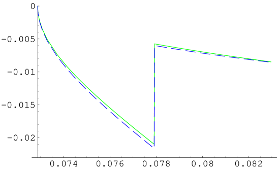
$s_{3}\ ({\rm GeV^{2}})$

Figure 3: Plot of $\frac{N}{|C^{\prime}|^{2}}\,\frac{d\Gamma_{\rm cusp}/ds_{3}}{v_{\pm}(s_{3})}$ around threshold as a function of $s_{3}$, $4m_{\pi^{0}}^{2}\leq s_{3}\leq 4(2m_{\pi^{+}}^{2}-m_{\pi^{0}}^{2})$, for the decay $K^{+}\rightarrow\pi^{0}\pi^{0}\pi^{+}$. The meaning of the various lines is explained in the text.

In Figure 3, we show the cusp effect for $K^{+}\to\pi^{0}\pi^{0}\pi^{+}$ at NLO. The solid line is our result for $\frac{N}{|C^{\prime}|^{2}}\,\frac{d\Gamma_{\rm cusp}/ds_{3}}{v_{\pm}(s_{3})}$ in (53) using (4.1). Effective $\pi\pi$ scattering lengths near threshold in (4) are unknowns to be fixed by fitting the cusp effect, however for the numerical comparison we take them as inputs given by CHPT [20] at NLO. For the rest of inputs needed for $\rm Re\overline{A}_{00+}$ and $\rm Re\overline{A}_{++-}$ we use the ones in Appendix A, which have been obtained from a fit to data.

Using the same value of the $\pi\pi$ scattering lengths, we also plot $\frac{N}{|C^{\prime}|^{2}}\,\frac{d\Gamma_{\rm cusp}/ds_{3}}{v_{\pm}(s_{3})}$ in Figure 3 as obtained using the results in [16] –this is the dashed curve. For the slopes needed for $\mbox{Re}A_{00+}$ and $\mbox{Re}A_{++-}$ in (4.6) and (4.7) in [16], we use the Taylor expansion of our NLO in CHPT results for $\mbox{Re}A_{00+}$ and $\mbox{Re}A_{++-}$. This makes the comparison with the solid curve clearer. The effect of using instead the slopes from Taylor expanding $|\mbox{Re}A_{00+}|^{2}+|\mbox{Im}A_{00+}|^{2}$ and $|\mbox{Re}A_{++-}|^{2}+|\mbox{Im}A_{++-}|^{2}$, respectively, amounts to a further increase of the difference between solid and dashed curves by around 2 % below threshold and 1 % above threshold. Notice that from a fit to data one can just access the slopes from $|\mbox{Re}A_{00+}|^{2}+|\mbox{Im}A_{00+}|^{2}$ and $|\mbox{Re}A_{++-}|^{2}+|\mbox{Im}A_{++-}|^{2}$.

If one compares the dashed and the solid curves in Figure 3, one gets differences below threshold around 3 % while above threshold vary between 2.5 % and 1 %. They come from several order 1% approximations done in [16] which we have identified and enumerate below.

The piece $\mbox{Im}\overline{A}_{00+}\,\mbox{Re}\overline{B}_{00+}$, –which we include in the numerics and it was not in [16]– is nominally order $a^{3}$ and contributes to the cusp below threshold by less than 1 %. Notice that this term contains a suppressing velocity factor $v_{00}(s_{3})$. Using a quadratic polynomial in $s_{3}$ as in [16] instead of the exact NLO CHPT formula is a very good approximation and gives differences smaller than 0.5 %.

As said above, the difference between doing an integral in $x$ or $y$ in (4.1), (61) and (62) numerically and doing the linear approximation is around 1 % each. Since the cusp formula in (53) is quadratic some of these differences are actually doubled. At the end of the day, these individually negligible approximations produce the final differences between dashed and solid curves quoted above and seen in Figure 3. Notice that we don’t get the final difference by summing the individual ones, it just happens that they go in the same direction.

This provides a first handle on the theoretical uncertainty of the Cabibbo’s approach to obtain the scattering lengths since the differences quoted above do not affect the treatment of $\pi\pi$ scattering.

Let us now estimate the theoretical uncertainty in our approach of determining the effective scattering length $a_{x}(s_{3})$ in (4). There are two main sources of theoretical uncertainties. One is how good is the fit of NLO CHPT formulas to experimental data. In case of using CHPT NLO formulas for $\mbox{Re}\,\overline{A}_{00+}$, this fit produces central values which agree with experiment within $3\%$ accuracy [5, 9]. This global fit was done using total decay rates and Dalitz variable slopes. We want to remark that this fit of $\mbox{Re}\,\overline{A}_{00+}$ to data has to be good enough also away from threshold. Notice that, for instance, in (4.1) one needs $\mbox{Re}\,\overline{A}_{00+}$ evaluated at $a(s_{3})$ which is typically around $(m_{K}^{2}-m_{\pi}^{2})/2$.

The other main source of uncertainty, which is more difficult to estimate and that is present in any approach which describes the cusp effect to NLO, is the NNLO corrections. The only definite way to know it is to calculate these corrections. In our approach, this means to calculate the real part of $K^{+}\to\pi^{0}\pi^{0}\pi^{+}$ at two-loop in the isospin conserving limit and make the same analysis that we have done but at NNLO. Notice that in this analysis the two-pion phase space factors are the physical ones in order to describe the cusp effect.

Meanwhile, we can just make the following estimate. Going from one order to the next one in our approach implies that new topologies with an extra $\pi\pi$ scattering vertex are needed. For instance, topology C in Figure 1 appears when going from LO to NLO, and analogously there appear new topologies when going from NLO to NNLO. Following this line, a naive estimate of NNLO re-scattering effects in $K\to 3\pi$ is that they are suppressed with respect to LO by $a_{i}^{2}$. Notice that the velocity factors that appear after applying the unitarity cuts can be order one –see for instance (4.1), where $v_{\pm}(a(4m_{\pi}^{2}))\simeq 0.6$– and do not suppress the naive $a_{i}^{2}$ estimate. Our estimate coincides numerically with the one made in [16], i.e. it gives around 5 % corrections from NNLO contributions. As said above, at NNLO it is possible to follow a procedure analogous to the one we use here to get a more accurate measurement of $a_{0}-a_{2}$ and check the estimated NNLO uncertainty.

If the theoretical uncertainty from the fit is added to the 5 % of canonical uncertainty assigned to NNLO we get a theoretical uncertainty in our approach of obtaining the scattering lengths from the cusp effect in $K^{+}\to\pi^{0}\pi^{0}\pi^{+}$ between somewhat larger than 5 % (if uncertaintities are added quadratically) and 7 % (if added linearly), i.e., we essentially agree therefore with the uncertainty quoted by [16].

A further source of error in the final determination of the scattering length $a_{0}-a_{2}$ from a fit to the cusp effect below threshold is due, as already discussed in [16], to the existence of different strategies to do the fit. The three basic ones are:

• One can consider all the $a_{i}$ as free parameters in (4.1).

• All $a_{i}$ are fixed to their standard values except the combination $a_{0}-a_{2}$ in $a_{x}$ that is extracted from the fit.

• One can use CHPT as much as possible. Since the combination $a_{0}-a_{2}$, or equivalently $a_{x}(s_{3})$, only appears in $\overline{B}_{00+}$, which is proportional to the cusp, it is enough to keep $\overline{B}_{00+}$ in terms of the scattering lengths. So that, one could fully use the CHPT predictions at NLO in [5, 9] for Im $\overline{A}_{00+}$.

The comparison of the results for $a_{x}$ obtained from these different fit strategies will provide us with another handle to estimate the accuracy of the method. This uncertainty will become clear once the fits that we propose are done with data and to be added to the previous ones. To the uncertainties discussed above, one still has to add the one here from the different data fitting strategies.

4.2 Cabibbo’s Proposal for Neutral Kaons

In the neutral kaon channel it is also possible to measure the scattering lengths combination $a_{0}-a_{2}$ from the cusp effect in the energy spectrum of two $\pi^{0}$ of $K_{L}\to\pi^{0}\pi^{0}\pi^{0}$. In this case the Bose symmetry of the three neutral pions implies that the amplitude is completely symmetric for the interchanges $s_{1}\leftrightarrow s_{2}\leftrightarrow s_{3}$. The amplitude near $\pi^{+}\pi^{-}$ threshold can be written as [16]

$$A_{000} = \left\{\begin{array}[]{ll}\sum\limits_{i=1,2,3}\left[\overline{A}_{000}(s_{i})+v_{\pm}(s_{i})\overline{B}_{000}(s_{i})\right]\ ,&{\rm if\,\,all\,\,}s_{i}>4m_{\pi^{+}}^{2}\ ;\\ \\ \left\{\sum\limits_{i=1,2,3}\overline{A}_{000}(s_{i})\right\}+\,i\,v_{\pm}(s_{k})\overline{B}_{000}(s_{k})&\\ +\sum\limits_{\scriptstyle\begin{array}[]{l}\scriptstyle{i=1,2,3}\\ \scriptstyle{i\neq k}\end{array}}v_{\pm}(s_{i})\overline{B}_{000}(s_{i})\ ,&\left\{\begin{array}[]{l}\quad{\rm for}\quad s_{k}<4m_{\pi^{+}}^{2},\\ k=1,2,3\\ \quad{\rm for}\quad s_{i\neq k}>4m_{\pi^{+}}^{2}\ .\end{array}\right\}\end{array}\right.$$ (77)

The crucial observation in (77) is that if the value of $s_{k}$ is below threshold, the other two variables $s_{i}$ ($i\neq k$) are of order $(m_{K}^{2}-m_{\pi}^{2})/2$, so safely above threshold. Thus it is kinematically impossible to cross the threshold with all three variables $s_{i}$ at the same time.

In the region where $s_{3}$ is around threshold, one can define

$$\overline{A}_{000}^{\prime}(s_{1},s_{2},s_{3}) = \sum_{i=1,2,3}\overline{A}_{000}(s_{i})+\sum_{i=1,2}v_{\pm}(s_{i})\overline{B}_{000}(s_{i})\ ,$$

$${\rm and}\quad\quad\overline{B}_{000}^{\prime}(s_{3}) = \overline{B}_{000}(s_{3})\ .$$ (78)

Equations (49)-(53) are now valid also for the decay of $K_{L}\rightarrow\pi^{0}\pi^{0}\pi^{0}$ once the substitutions $A_{00+}\rightarrow A_{000}$, $\overline{A}_{00+}\rightarrow\overline{A}_{000}^{\prime}$ and $\overline{B}_{00+}\rightarrow\overline{B}_{000}^{\prime}$ are done.

Again, we write these amplitudes using the approximation (4) for the amplitudes near threshold. The amplitudes contain $\pi\pi$ re-scattering in all channels and in those channels where they are far from threshold we use full NLO CHPT expressions which, as already pointed out in Section 4, is a better approximation than the effective scattering lengths.

The calculation of $\overline{A}_{000}^{\prime}$ and $\overline{B}_{000}^{\prime}$ is completely analogous to the charged kaon case – see Section 4.1. Using the tree-level result for the real part of $K_{L}\to\pi^{0}\pi^{0}\pi^{0}$, one finds

$$\mbox{Re}{\overline{A}_{000}^{\prime}}|_{LO} = C^{\prime}\,(\mbox{Re}\,G_{8}-G_{27})m_{K}^{2},$$

$$\mbox{Im}{\overline{A}_{000}^{\prime}}|_{LO}(s_{1},s_{2},s_{3}) = \mbox{Re}{\overline{A}_{000}^{\prime}}|_{LO}\left[v_{00}(s_{3})a_{00}(s_{3})+\,\sum_{i=1,2}v_{00}(s_{i})\frac{m_{\pi}^{2}}{32\pi^{2}f_{\pi}^{2}}\right]$$

$$+\sum_{i=1,2}v_{\pm}(s_{i})\,\frac{s_{i}-m_{\pi}^{2}}{16\pi f_{\pi}^{2}}\,f_{000}(s_{i})\ ,$$

$$\mbox{Re}{\overline{B}_{000}^{\prime}}|_{LO}(s_{3}) = 0\,,$$ (79)

$$\mbox{Im}{\overline{B}_{000}^{\prime}}|_{LO}(s_{3}) = 2a_{x}(s_{3})f_{000}(s_{3})\ ,$$ (80)

with

$$f_{000}(s) = C^{\prime}\left[\mbox{Re}\,G_{8}\left(s-m_{\pi}^{2}\right)+\frac{G_{27}}{6(m_{K}^{2}-m_{\pi}^{2})}\left(s(9m_{K}^{2}-24m_{\pi}^{2})-5m_{K}^{4}\right.\right.+$$ (81)

$$\left.+24m_{\pi}^{4}+m_{\pi}^{2}m_{K}^{2}\right)\Big{]}\ .$$

The meaning of $LO$ here is the same that in (4.1).

The effect of the charged pion re-scattering appears also at NLO. At this order we use the CHPT one-loop formula for $\mbox{Re}\overline{A}_{000}^{\prime}$ fitted to data. We get

$$\mbox{Re}{\overline{A}_{000}^{\prime}}|_{NLO}(s_{1},s_{2},s_{3}) = \mbox{Re}{\overline{A}_{000}^{\prime}}|_{LO}+\Big{[}M_{0}(s_{1})+M_{0}(s_{2})+M_{0}(s_{3})\Big{]}_{{\cal O}(p^{4})}+$$

$$+\delta\mbox{Re}\overline{A}_{000}^{\prime}(s_{1},s_{2},s_{3})\,,$$

$$\mbox{Im}{\overline{A}_{000}^{\prime}}|_{NLO}(s_{1},s_{2},s_{3}) = \mbox{Im}{\overline{A}_{000}^{\prime}}|_{LO}\,+\,v_{00}(s_{3})a_{00}(s_{3})\Big{[}M_{0}(s_{3})+\widetilde{M}_{0}(s_{3})\Big{]}_{{\cal O}(p^{4})}+$$

$$+\Big{[}{\rm Im}A^{(6,1)}_{W}(s_{1})+{\rm Im}A^{(6,2)}_{W}(s_{1})+{\rm Im}A^{(6,1)}_{\pi}(s_{1})+{\rm Im}A^{(6,2)}_{\pi}(s_{1})+$$

$$\hskip 28.45274pt+s_{1}\leftrightarrow s_{2}\Big{]}\,,$$

$$\mbox{Re}{\overline{B}_{000}^{\prime}}|_{NLO}(s_{3}) = F_{000}(s_{3})\,,$$

$$\mbox{Im}{\overline{B}_{000}^{\prime}}|_{NLO}(s_{3}) = \mbox{Im}{\overline{B}_{000}^{\prime}}|_{LO}\,+\,2a_{x}(s_{3})\left[M_{1}(s_{3})+\widetilde{M}_{2}(s_{3})+\right.$$

$$\left.+\widetilde{M}_{3}(s_{3})(m_{K}^{2}+3m_{\pi}^{2}-2s_{3})-\widetilde{M}_{3}^{s}(s_{3})\right]_{{\cal O}(p^{4})}\,,\quad$$

where we neglected the contributions of three-pion cut graphs which have been shown to be very small in Appendix C. The function $F_{000}(s)$ has the expression

$$F_{000}(s) = -a_{00}(s)v_{00}(s)\,\mbox{Im}\overline{B}_{000}(s)$$

$$-2a_{x}(s)^{2}v_{00}(s)\,\Big{\{}\mbox{Re}{\overline{A}_{000}}\left(s\right)+{\displaystyle\int_{-1}^{1}}\,{\rm d}x\,\mbox{Re}{\overline{A}_{000}}\left(t^{+}(s,x)\right)\Big{\}}\,$$

$$-a_{x}(s){\displaystyle\int_{-1}^{1}}\,{\rm d}x\,\mbox{Im}\tilde{A}_{+-0}^{L}(t^{+}(s,x),t^{-}(s,x))\,\,.$$

The first two lines here come from diagram B in Figure 1 while the last line comes solely from diagram C in the same figure.

As already discussed in the case of the analogous calculation of the discontinuity for the charged $K^{+}\to\pi^{0}\pi^{0}\pi^{+}$ decay in Section 4.1, the integration contour along the real axis $-1\leq x\leq 1$ in $F_{000}(s)$ gives the correct result just for small values of $s$, namely [23], for

$$4m_{\pi^{0}}^{2}\leq s\leq\frac{1}{2}\left(m_{K^{0}}^{2}-m_{\pi^{0}}^{2}\right)\,.$$ (83)

For larger values of $s$ there is an additional piece [23] and the same comments and discussion around (60) apply here.

The functions ${\rm Im}A^{(6,i)}_{j}(s)$ are given in Appendix B.2 and the meaning of $NLO$ in (4.2) is the same that in (4.1). The imaginary part of the $K_{L}\to\pi^{+}(p_{1})\pi^{-}(p_{2})\pi^{0}(p_{3})$ decay amplitude, $\mbox{Im}A_{+-0}^{L}(t_{1},t_{2},t_{3})$, has been obtained here using the optical theorem. See Section 3 and Appendix B.3 for the full expression. From that result, disregarding the tiny contribution from the P wave and the pieces that do not contribute to singularities, the function $\mbox{Im}\tilde{A}_{+-0}^{L}(t_{1},t_{2})$ is

$$\mbox{Im}\tilde{A}_{+-0}^{L}(t_{1},t_{2})=a_{+0}(t_{1})v_{+0}(t_{1}){\displaystyle\int_{-1}^{1}}\,{\rm d}y\,\mbox{Re}{\overline{A}_{+-0}^{L}}(t_{1},t^{+}(t_{1},y),t^{-}(t_{1},y))+\,t_{1}\rightarrow t_{2}\,,$$ (84)

where the expression for $\mbox{Re}{\overline{A}_{+-0}^{L}}$ at NLO in CHPT can be found in [5, 9]. This expression has to be fitted to $K_{L}\to\pi^{+}\pi^{-}\pi^{0}$ data. Notice that, in the formula above, $\pi\pi$ amplitudes are sometimes evaluated far from threshold. As explained at the introduction of Section 4, whenever this happens we use full NLO CHPT predictions for the $\pi\pi$ scattering amplitudes and not the effective scattering length combinations near threshold in (4).

The contribution $\delta\mbox{Re}{\overline{A}_{000}^{\prime}}$ comes from the discontinuity across the physical cuts and takes into account just the singularities of $\mbox{Re}{\overline{A}_{000}^{\prime}}$ at $s_{i}=4m_{\pi^{+}}^{2}$, $s_{i}=(m_{\pi^{+}}+m_{\pi^{0}})^{2}$ and $s_{i}=4m_{\pi^{0}}^{2}$ ($i=1,2$) thresholds. These singularities start at order $p^{6}$ in CHPT. We get

$$\delta\mbox{Re}{\overline{A}_{000}^{\prime}}(s_{1},s_{2},s_{3}) = {\displaystyle\sum_{i=1,2}}v_{\pm}(s_{i})\,F_{000}(s_{i})-\,{\displaystyle\sum_{i=1,2,3}}v_{00}(s_{i})\,a_{00}(s_{i})$$ (85)

$$\times\,{\displaystyle\int_{-1}^{1}}\,{\rm d}x\;\Bigg{\{}\,a_{00}(t^{+}(s_{i},x))v_{00}(t^{+}(s_{i},x))\Big{[}{\mbox{Re}\overline{A}_{000}}(t^{+}(s_{i},x))$$

$$+{\displaystyle\int_{-1}^{1}}\,{\rm d}y\;{\mbox{Re}\overline{A}_{000}}(t^{+}(t^{+}(s_{i},x),y))\Big{]}+a_{x}(t^{+}(s_{i},x))v_{\pm}(t^{+}(s_{i},x))$$

$$\times{\displaystyle\int_{-1}^{1}}\,{\rm d}y\;\mbox{Re}{\overline{A}_{+-0}}(t^{+}(t^{+}(s_{i},x),y),t^{-}(t^{+}(s_{i},x),y),t^{+}(s_{i},x))\,\Bigg{\}}\,.$$

Here, the same comments after (4.1) apply. I.e., the integration contour $-1\leq x\leq 1$ gives the correct result just when both $s_{3}$, $s_{1}$ and $s_{2}$ are all in the range in (83) –remember that $s_{3}$ is always around threshold. For values of $s_{1}$ or $s_{2}$ outside (83) the same discussion after (4.1) applies.

In [16], they used the approximation that the integrands in (4.2), (84) and (85) are to a good accuracy linear in the variables $x$ and $y$ . If we make such approximation, we get

$$\mbox{Re}\overline{B}_{000}^{\prime}|_{NLO}(s_{3}) = -a_{00}(s_{3})v_{00}(s_{3})\mbox{Im}{\overline{B}_{000}}(s_{3})$$ (86)

$$-2\,a_{x}(s_{3})^{2}v_{00}(s_{3})\Big{\{}\mbox{Re}{\overline{A}_{000}}\left(s_{3}\right)+2\,\mbox{Re}{\overline{A}_{000}}\left(a(s_{3})\right)\Big{\}}$$

$$-8a_{x}(s_{3})a_{+0}(a(s_{3}))v_{+0}(a(s_{3}))\mbox{Re}{\overline{A}_{+-0}^{L}}(a(s_{3}),a(a(s_{3})),a(a(s_{3})))$$

$$\delta\mbox{Re}{\overline{A}_{000}^{\prime}}(s_{1},s_{2},s_{3}) = -{\displaystyle\sum_{i=1,2}}\,v_{\pm}(s_{i})\,\Big{\{}a_{00}(s_{i})v_{00}(s_{i})\mbox{Im}{\overline{B}_{000}}(s_{i})+$$ (87)

$$+2\,a_{x}(s_{i})^{2}v_{00}(s_{i})\Big{[}\mbox{Re}{\overline{A}_{000}}\left(s_{i}\right)+2\,\mbox{Re}{\overline{A}_{000}}\left(a(s_{i})\right)\Big{]}$$

$$+8a_{x}(s_{i})a_{+0}(a(s_{i}))v_{+0}(a(s_{i}))\mbox{Re}{\overline{A}_{+-0}^{L}}(a(s_{i}),a(a(s_{i})),a(a(s_{i})))\Big{\}}$$

$$-2\sum_{i=1,2,3}a_{00}(s_{i})v_{00}(s_{i})\Big{\{}a_{00}\left(a(s_{i})\right)v_{00}\left(a(s_{i})\right)\left[\mbox{Re}\overline{A}_{000}(s_{i})+2\,\mbox{Re}\overline{A}_{000}\left(a(s_{i})\right)\right]$$

$$+2a_{x}(a(s_{i}))v_{\pm}(a(s_{i}))\mbox{Re}{\overline{A}_{+-0}^{L}}\left(a\left(a(s_{i})\right),a\left(a(s_{i})\right),a(s_{i})\right)\Big{\}}$$

which agree with [16] up to the terms proportional to $v_{00}(a(s_{i}))$ and $v_{\pm}(a(s_{i}))$ in $\delta\mbox{Re}{\overline{A}_{000}^{\prime}}$, which were not included there.

$\small{100\times}\frac{{\rm d}|\Gamma_{\rm cusp}(s_{3})|/{\rm d}s_{3}}{{\rm d}\Gamma(s_{3})/{\rm d}s_{3}}$

$s_{3}({\rm GeV}^{2})$

Figure 4: Plot of $100\times\frac{{\rm d}|\Gamma_{\rm cusp}(s_{3})|}{{\rm d}s_{3}}$ over $\frac{{\rm d}\Gamma(s_{3})}{{\rm d}s_{3}}$ around threshold as a function of $s_{3}$, $4m_{\pi^{0}}^{2}\leq s_{3}\leq 4(2m_{\pi^{+}}^{2}-m_{\pi^{0}}^{2})$, for the decay $K_{L}\rightarrow\pi^{0}\pi^{0}\pi^{0}$.

In Figure 4 we show the ratio $100\times\frac{{\rm d}|\Gamma_{\rm cusp}(s_{3})|}{{\rm d}s_{3}}$ over $\frac{{\rm d}\Gamma(s_{3})}{{\rm d}s_{3}}$ using the results in (4.2) for $K_{L}\rightarrow\pi^{0}\pi^{0}\pi^{0}$. Here, $\Gamma_{\rm cusp}$ is the contribution of $v_{\pm}(s_{3})\Delta_{\rm cusp}(s_{1},s_{3})$ in (53) to the total $K_{L}\to\pi^{0}\pi^{0}\pi^{0}$ decay rate $\Gamma$. We perform the integrals in $x$ and $y$ in (4.2), (84) and (85) numerically.

For the sake of numerical comparison with the results in [16], we do not include the additional pieces discussed after (83) in the integral over $s_{1}$ in (67) defining ${{\rm d}|\Gamma_{\rm cusp}(s_{3})|}/{{\rm d}s_{3}}$, which were also not included in that reference either. An analogous discussion to the one after (67) applies in this case as well.

In Figure 5 we plot the cusp effect $\frac{3N}{|C^{\prime}|^{2}}\,\,\frac{d\Gamma_{\rm cusp}/ds_{3}}{v_{\pm}(s_{3})}$ in (53) for $K_{L}\to\pi^{0}\pi^{0}\pi^{0}$ at NLO. The solid line are our results in (4.2). We use the same inputs as for the charged case in the previous section.

$\frac{3N}{|C^{\prime}|^{2}}\,\,\frac{d\Gamma_{\rm cusp}/ds_{3}}{v_{\pm}(s_{3})}({\rm GeV}^{6})$

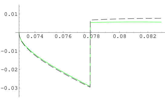
$\quad\quad\quad s_{3}({\rm GeV^{2}})$

Figure 5: Plot of $\frac{3N}{|C^{\prime}|^{2}}\,\,\frac{d\Gamma_{\rm cusp}/ds_{3}}{v_{\pm}(s_{3})}$ around threshold as a function of $s_{3}$, $4m_{\pi^{0}}^{2}\leq s_{3}\leq 4(2m_{\pi^{+}}^{2}-m_{\pi^{0}}^{2})$ for the decay $K_{L}\rightarrow\pi^{0}\pi^{0}\pi^{0}$. The meaning of the various lines is explained in the text.

We also plot in Figure 5, the cusp effect $\frac{3N}{|C^{\prime}|^{2}}\,\frac{d\Gamma_{\rm cusp}/ds_{3}}{v_{\pm}(s_{3})}$ using the results in [16] –this is the dashed curve. For the slopes needed for $\mbox{Re}A_{000}^{L}$ and $\rm ReA_{+-0}^{L}$ in (4.58) and (4.59) in [16], we use the Taylor expansion of our results for $\mbox{Re}A_{000}^{L}$ and $\mbox{Re}A_{+-0}^{L}$. This makes the comparison with the solid curve clearer. The numerical differences between solid and dashed curves increase by around 2 % if instead we use the slopes from Taylor expanding $|\mbox{Re}A_{000}^{L}|^{2}+|\mbox{Im}A_{000}^{L}|^{2}$ and $|\mbox{Re}A_{+-0}^{L}|^{2}+|\mbox{Im}A_{+-0}^{L}|^{2}$, respectively.

If one compares the dashed and solid curves below threshold in Figure 5, one gets differences between 3 % and 1 %. As for the charged case, we have identified the origin of these differences: they come from several order 1% approximations done in [16]. Notice that we don’t add them, it just happens that they go in the same direction. The part of the singularities in $\delta\mbox{Re}\overline{A}_{000}^{\prime}$ that was not included in [16] –see comment after (87)– and that we do include in the solid line contributes about +1.5 % to this difference. The other approximations are analogous to the ones already enumerated for the charged case –see previous section. For instance, the piece $\mbox{Im}\overline{A}_{000}^{\prime}\,\mbox{Re}\overline{B}^{\prime}_{000}$ –which we include and it was not in [16]– is nominally order $a^{3}\,v_{\pm}(s_{3})$ and contributes to the cusp below threshold by around 1 %. Again, at the end of the day, these individually negligible approximations produce the final differences between dashed and solid curves quoted above.

Notice again that the differences between our approach and the one in [16] do not affect the treatment of the $\pi\pi$ scattering part.

Above threshold, there are large numerical cancellations between $\mbox{Im}\overline{A}^{\prime}_{000}\,\mbox{Im}\overline{B}^{\prime}_{000}$ and $\mbox{Re}\overline{A}^{\prime}_{000}\,\mbox{Re}\overline{B}^{\prime}_{000}$ in the corresponding expression for $\Delta_{\rm cusp}$ in $K_{L}\to\pi^{0}\pi^{0}\pi^{0}$ –see (53) for the analogous charged case. As a consequence, one should know both the real and imaginary parts of $\overline{A}^{\prime}_{000}$ and $\overline{B}^{\prime}_{000}$ with a precision better than 1 % to predict the cusp above threshold with an uncertainty around 5 %. The observed difference between the two curves above threshold in Figure 5 is due to the need of this fine tuning and is not physical. This fact makes the region above threshold not suitable to extract the scattering lengths in $K_{L}\to\pi^{0}\pi^{0}\pi^{0}$.

Let us now estimate the theoretical uncertainty in our approach of determining the effective scattering length $a_{x}(s_{3})$ in (4) from $K_{L}\to\pi^{0}\pi^{0}\pi^{0}$. As for the charged case, one has the theoretical uncertainty from the fitting to $\mbox{Re}\overline{A}_{000}$ which includes the theoretical error which measures the accuracy of the formula used to do the fit. As said above, this has to be checked once the real fit is done but we believe that it is realistic to assume that this theoretical uncertainty is around 2 %. Again, the accuracy of the data should be at the level of a few per cent as for the charged case.

If this is added to the 5 % of canonical uncertainty assigned to NNLO we get a theoretical uncertainty for the scattering lengths combination $a_{0}-a_{2}$ from the cusp effect in $K_{L}\to\pi^{0}\pi^{0}\pi^{0}$ between somewhat larger than 5 % (if uncertainties are added quadratically) and 7 % (if added linearly). I.e., we predict a similar theoretical accuracy in the extraction of $a_{0}-a_{2}$ from neutral and charged kaon cusp effects. But notice that in the neutral case, this uncertainty just applies to the analysis of the data below threshold. As said before, there are very large numerical cancellations above threshold which preclude the use of these data.

To the uncertainties discussed above, one still has to add the one from the different data fitting strategies as described in Section 4.1.

5 Summary and Conclusions

In Section 3, we have presented the full FSI phases for all $K\to 3\pi$ decays at NLO in CHPT, i.e. at ${\cal O}(p^{6})$ analytically. The two-pion cut contributions for $K^{+}\to 3\pi$ were already presented in [5]. We complete the calculation here with the three-pion cut contributions and the full result for $K_{L,S}\to 3\pi$. The two-pion cut contributions are given analytically while the three-pion cut ones are done numerically and checked always to be negligible. We used the techniques already explained in [5] which are based on perturbative unitarity and analyticity of CHPT.

In Section 4.1, we study Cabibbo’s proposal to measure the scattering lengths combination $a_{0}-a_{2}$ from the cusp effect in the total $\pi^{0}\pi^{0}$ pair energy spectrum in $K^{+}\to\pi^{0}\pi^{0}\pi^{+}$ [14, 16]. To be more specific, ours is a variation of the original Cabibbo’s proposal that uses NLO CHPT for the real part of $K\to 3\pi$ vertex instead of the quadratic polynomial in $s_{3}$ approximation used in [14, 16] plus analyticity and unitarity. We studied also the analogous proposal for $K_{L}\to\pi^{0}\pi^{0}\pi^{0}$ in Section 4.2.

Notice that we do not use CHPT to predict the real part of $K\to 3\pi$, but use its exact singularity form at NLO in CHPT to fit it to data above threshold. If the two-loop CHPT singularity structure was known it could be used in order to take this singularity structure exactly in $\mbox{Re}\overline{A}_{00+}$. The treatment of $\pi\pi$ scattering near threshold is independent of this choice and we treat it in the same way as in [16]. See the introduction of Section 4.

The cusp effect originates in the different contributions to $K^{+}\to\pi^{0}\pi^{0}\pi^{+}$ and $K_{L}\to\pi^{0}\pi^{0}\pi^{0}$ amplitudes above and below threshold of $\pi^{+}\pi^{-}$ production in the $\pi^{0}\pi^{0}$ pair invariant energy. We obtain these contributions using just analyticity and unitarity, in particular applying Cutkosky rules and the optical theorem above and below threshold to calculate the discontinuity across the physical cut. This allows us to separate $\pi\pi$ scattering –which we want to measure– from the rest of $K^{+}\to\pi^{0}\pi^{0}\pi^{+}$ or $K_{L}\to\pi^{0}\pi^{0}\pi^{0}$.

We would like to remark here that making the same approximations that were done in [16] we fully agree with their analytical results. In particular, we checked that the use of the quadratic polynomial in $s_{3}$ in [16] instead of CHPT formulas at NLO produce negligible differences –around 0.5 %– in $\Delta_{\rm cusp}$ in (53).

The real part of the discontinuity has a singularity when any of the $s_{i}$ invariant energy reaches its pseudo-threshold at $(m_{K}-m_{\pi^{(i)}})^{2}$ as described in [23]. We have discussed how this singularity appears in our formulas for the discontinuity and discussed its effects in the description of the cusp effect using the discontinuity –see Section 4.1 and Section 4.2.

In particular, we pointed out that while the presence of that singularity at pseudo-thresholds does not affect $\mbox{Re}\overline{B}_{00+}(s_{3})$ in (4.1) and $\mbox{Re}\overline{B}_{000}^{\prime}(s_{3})$ in (4.2) when $s_{3}$ is around threshold, one needs to take fully into account its effects for $\delta\mbox{Re}{\overline{A}_{00+}}$ in (62) and (66) and $\delta\mbox{Re}{\overline{A}_{000}^{\prime}}$ in (85) and (87) when $s_{1}$ or $s_{2}$ is above $(m_{K}^{2}-m_{\pi}^{2})/2$. For a possible solution of this problem which does not simply use the discontinuity to describe the cusp effect see [22]. Another possibility could be to use, instead of $\delta\mbox{Re}{\overline{A}_{00+}}$ and $\delta\mbox{Re}{\overline{A}_{000}^{\prime}}$, the full-two loop (not available yet) finite relevant pieces to describe the singularities at thresholds at NLO in $\mbox{Re}{\overline{A}_{00+}}$ and $\mbox{Re}{\overline{A}_{000}^{\prime}}$, respectively. This could be fitted to data since we don’t want to predict $\mbox{Re}{\overline{A}_{00+}}$ and $\mbox{Re}{\overline{A}_{000}^{\prime}}$ but to obtain the best description of them. We leave a more detailed study of this problem and possible solutions for a future work.

In Sections 4.1 and 4.2 we have also discussed some approximations done in [16] and the numerical differences they induce in $\Delta_{\rm cusp}$ in (53). See Figure 3 and Figure 5 and text around. We have identified them and found that though each one of them is individually negligible (between 0.5 % to 1 %) they produce final differences in the $\Delta_{\rm cusp}$ around 3 %.

In the same sections, the theoretical uncertainties in the determination of $a_{0}-a_{2}$ if one uses our formulas to fit the experimental data are discussed. We concluded that for $K^{+}\to\pi^{0}\pi^{0}\pi^{+}$, this uncertainty is somewhat larger than 5 % if uncertainties are added quadratically and 7 % if added linearly. I.e., we essentially agree with the estimate in [16]. Notice that we get our final theoretical uncertainty as the sum of several order 1% to 2% uncertainties to the canonical NNLO 5 % uncertainty.

For the case $K_{L}\to\pi^{0}\pi^{0}\pi^{0}$, we get that –if one uses just data below threshold– the uncertainty in the determination of $a_{0}-a_{2}$ is of the same order as for $K^{+}\to\pi^{0}\pi^{0}\pi^{+}$. Above threshold, we found large numerical cancellations which preclude from using it.

An expansion in the scattering lengths $a_{i}$ and Feynman diagrams were used in [16] to do the power counting and obtain the cusp effect description of $K^{+}\to\pi^{0}\pi^{0}\pi^{+}$ at NLO. In general, when FSI $\pi\pi$ scattering effects are included at $n$-th order, there appear new topologies in $K\to 3\pi$ –topology C at NLO order, for instance– which give contributions to $\Delta_{\rm cusp}$ of order $a_{i}^{n}$. The canonical uncertainty of the $n$-th order results is thus $a_{i}^{n}$. Notice that the velocity factors that appear after applying the unitarity cuts can be order one –see for instance (4.1), where $v_{\pm}(a(4m_{\pi}^{2}))\simeq 0.6$– and do not suppress the naive $a_{i}^{n}$ estimate.

Our estimate for the uncertainty from NNLO, $\sim a_{i}^{2}$, coincides numerically with the one made in [16],i.e. it gives around 5 %. We conclude that one cannot expect to decrease this canonical $5\%$ theoretical uncertainty of the NLO result unless one includes $\pi\pi$ scattering effects at NNLO. If one wants to reach the per cent level in the uncertainty of the determination of $a_{0}-a_{2}$ from the cusp effect, one would need to include those NNLO re-scattering effects. As said above, at NNLO it is possible to follow a procedure analogous to the one we use here to get a more accurate measurement of $a_{0}-a_{2}$ and check the estimated NNLO uncertainty.

We have just included isospin breaking due to the different thresholds using two-pion physical phase spaces in the optical theorem and Cutkosky rules. This is needed to describe the cusp effect. The rest of NLO isospin breaking is expected to be important just at NNLO. At that order, isospin breaking effects in $\pi\pi$ scattering at threshold –both from quark masses and from electromagnetism– will have to be implemented and their uncertainties added.

Finally, we believe that it is interesting to continue investigating the proposal in [14, 16] to measure the non-perturbative $\pi\pi$ scattering lengths from the cusp effect in $K^{+}\to\pi^{0}\pi^{0}\pi^{+}$ and $K_{L}\to\pi^{0}\pi^{0}\pi^{0}$. Another interesting direction is to develop an effective field theory in the scattering lengths which could both check the results in [16] and allow to go to NNLO. This type of studies is already underway and firsts results were presented [19, 22].

Appendices

Appendix A Numerical Inputs

Here we discuss the numerical inputs we use in the numerical applications. In [9], a fit to all available $K\to\pi\pi$ amplitudes at NLO in CHPT and $K\to 3\pi$ amplitudes and slopes in $K\to 3\pi$ amplitudes was done. This was done in the isospin limit. More recently, this fit was updated in [13] with new data on slopes and including also the full isospin breaking effects. Though our calculation of FSI at NLO uses isospin limit results we will use the results obtained in this last fit. The reason is that the change in the fit results is due to both the new data used and the isospin breaking corrections at the same level and therefore cannot be disentangled. In addition, the main isospin breaking effects due to the kinematical factors is also taken into account in our results.

	$\mbox{Re}\widetilde{K}_{i}(M_{\rho})$ from [13]
$\widetilde{K}_{2}(M_{\rho})$	$G_{8}\times(48.5\pm 2.4)\cdot 10^{-3}$
$\widetilde{K}_{3}(M_{\rho})$	$G_{8}\times(2.6\pm 1.2)\cdot 10^{-3}$
$\widetilde{K}_{5}(M_{\rho})$	$-G_{27}\times(41.2\pm 16.9)\cdot 10^{-3}$
$\widetilde{K}_{6}(M_{\rho})$	$-G_{27}\times(102\pm 105)\cdot 10^{-3}$
$\widetilde{K}_{7}(M_{\rho})$	$G_{27}\times(78.6\pm 33)\cdot 10^{-3}$

Table 1: Results for the order $p^{4}$ counterterms $\mbox{Re}\,\widetilde{K}_{i}$ from the fit to data done in [13]. The values of $\mbox{Re}\,\widetilde{K}_{i}$ which do not appear are zero. For definitions of the counterterms, see [5, 9].

At order $p^{4}$, NLO in CHPT, the results in [13] are equivalent [using $F_{0}=87.7$ MeV] to

$$\mbox{Re}\,G_{8}=6.6\pm 1.1\hskip 14.22636pt{\rm and}\hskip 14.22636ptG_{27}=0.44\pm 0.09\,.$$ (88)

In this normalization, $\mbox{Re}\,G_{8}=1=G_{27}$ at large $N_{c}$. ($N_{c}$ is the number of colors of QCD).

For the NLO prediction of the FSI, we only need the real part of the counterterms and in particular the combinations in Table 1 of [5] which from the new fit in [13] are given in Table 1. These were obtained from a fit of the NLO in CHPT results to experimental data. Since we only want a good fit to data, one can fix them to any of these values which produce equally good fits.

Appendix B FSI Phases at NLO for Neutral Kaon Decays: Two-Pion Cuts

Here we include the analytical results for the two-pion cuts contributions to the dispersive part of the neutral decay amplitudes at NLO in CHPT, i.e. ${\cal O}(p^{6})$, coming from diagrams in Figure 6-7. Analogous results for the charged decay amplitudes as well as a more detailed description of the method, based on the use of the optical theorem, can be found in Appendix E of the first reference in [5]. The fully NLO FSI phases are completed by the calculation of the three-pion cut contributions, whose analytical results are given in Appendix C. In Subsections B.2, B.3 and B.4 we give the dispersive part of the amplitudes $A_{i}$ for $K_{L,S}\to 3\pi$ denoted by Im   $A^{6}_{i}$ where used the super-index $6$ to indicate the CHPT order.

B.1 Notation

In all the definitions and results written in this Appendix and in Appendices B.2, B.3 and B.4, the functions $M_{i}(t)$ and $P_{i}(t)$ are only the real part of the corresponding functions defined in [9] and [8] respectively. The expressions in Eqs. (B.2)-(112) are thus real.

We define

$$\widetilde{M}_{i}(s) = \int_{-1}^{1}{\rm d}x\;\left.M_{i}(a(s)+b(s)x)\right|_{p^{4}}\,,$$

$$\widetilde{M}_{i}^{s}(s) = \int_{-1}^{1}{\rm d}x\;\left.(a(s)+b(s)x)\,M_{i}(a(s)+b(s)x)\right|_{p^{4}}\,,$$

$$\widetilde{M}_{i}^{ss}(s) = \int_{-1}^{1}{\rm d}x\;\left.(a(s)+b(s)x)^{2}M_{i}(a(s)+b(s)x)\right|_{p^{4}}\,,$$ (89)

$${\rm with}\hskip 28.45274pta(s) = \frac{1}{2}(3s_{0}-s)+\frac{(m_{K}^{2}-m_{\pi^{(3)}}^{2})(m_{\pi^{(1)}}^{2}-m_{\pi^{(2)}}^{2})}{2s},$$

$${\rm and}\hskip 28.45274ptb(s) = \frac{1}{2s}\Big{\{}\Big{[}(s-(m_{\pi^{(1)}}+m_{\pi^{(2)}})^{2})(s-(m_{\pi^{(1)}}-m_{\pi_{(2)}})^{2})\Big{]}\times$$

$$\times\Big{[}(s-(m_{K}+m_{\pi^{(3)}})^{2})(s-(m_{K}-m_{\pi^{(3)}})^{2})\Big{]}\Big{\}}^{1/2}$$

for $s=(k-p_{3})^{2}$, see (2) for definition of these momenta.

The amplitudes at ${\cal O}(p^{4})$ for the $\pi\pi\rightarrow\pi\pi$ scattering in a theory with three flavors can be found in [8]. We decompose the amplitudes in the various cases as follows. For the case $\pi^{+}\pi^{+}\rightarrow\pi^{+}\pi^{+}$ the amplitude at ${\cal O}(p^{4})$ is

$$\Pi_{1} = P_{1}(s)+P_{2}(s,t)+P_{2}(s,u).$$ (91)

For the case $\pi^{0}\pi^{0}\rightarrow\pi^{+}\pi^{-}$ the amplitude at ${\cal O}(p^{4})$ is

$$\Pi_{2} = P_{3}(s)+P_{4}(s,t)+P_{4}(s,u).$$ (92)

For the case $\pi^{+}\pi^{-}\rightarrow\pi^{+}\pi^{-}$ the amplitude at ${\cal O}(p^{4})$ is

$$\Pi_{3} = P_{5}(s)+P_{6}(s,t)+P_{6}(s,u)+P_{7}(s,t)-P_{7}(s,u).$$

Finally, the amplitude $\pi^{0}\pi^{0}\rightarrow\pi^{0}\pi^{0}$ at ${\cal O}(p^{4})$ is

$$\Pi_{4} = P_{8}(s)+P_{8}(t)+P_{8}(u).$$ (94)

The value for the various $P_{i}$ can be obtained from [8]. In the following we use

$$\!\!\!\!\!\!\!\!\!\widetilde{P}^{(n,m)}_{i}(s) = s^{n}c(s)^{m}\,\int_{-1}^{1}{\rm d}x\;\,(1-x)^{m}\,P_{i}(s,c(s)(1-x)),$$

$$\!\!\!\!\!\!\!\!\!\hat{P}^{(n)}_{1,i}(s) = c(s)^{n}\,\int_{-1}^{1}{\rm d}x\;(1-x)^{n}\,P_{i}(c(s)(1+x),c(s)(1-x)),$$

$$\!\!\!\!\!\!\!\!\!\hat{P}^{(n)}_{2,i}(s) = c(s)^{n}\int_{-1}^{1}{\rm d}x\;(1-x)^{n}P_{i}(c(s)(1-x),s),$$ (95)

$$\!\!\!\!\!\!\!\!\!{\rm with}\hskip 28.45274ptc(s) = \frac{1}{2}(4m_{\pi}^{2}-s).$$ (96)

B.2 FSI for $K_{L}\rightarrow\pi^{0}\pi^{0}\pi^{0}$ at NLO

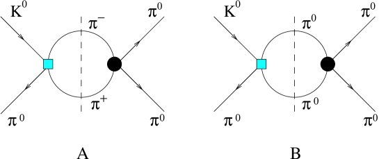
Figure 6: Diagrams for the calculation of FSI for $K_{L}\rightarrow\pi^{0}\pi^{0}\pi^{0}$ using the optical theorem. The square is the weak vertex and the circle is the strong one.

Diagrams A –two charged pions in the loop– and B –two neutral pions in the loop– in Figure 6 correspond to the two possible contributions for $K_{L}\to\pi^{0}\pi^{0}\pi^{0}$. We first compute the case when the weak vertex in Figure 6 is of ${\cal O}(p^{4})$ and the strong vertex of ${\cal O}(p^{2})$. The results are

$${\rm Im}A^{(6,1)}_{W}(s_{1},s_{2},s_{3}) = {\rm Im}A^{(6,1)}_{W}(s_{1})+{\rm Im}A^{(6,1)}_{W}(s_{2})+{\rm Im}A^{(6,1)}_{W}(s_{3})\,,$$

$${\rm Im}A^{(6,1)}_{W}(s) = \frac{\sigma(s)}{16\pi f_{\pi}^{2}}(s-m_{\pi}^{2})\left[M_{1}(s)+\widetilde{M}_{2}(s)+\widetilde{M}_{3}(s)(m_{K}^{2}+3m_{\pi}^{2}-2s)\right.-\left.\widetilde{M}_{3}^{s}(s)\right]_{{\cal O}(p^{4})}$$

$${\rm Im}A^{(6,2)}_{W}(s_{1},s_{2},s_{3}) = {\rm Im}A^{(6,2)}_{W}(s_{1})+{\rm Im}A^{(6,2)}_{W}(s_{2})+{\rm Im}A^{(6,2)}_{W}(s_{3})\,,$$

$${\rm Im}A^{(6,2)}_{W}(s) = \frac{\sigma(s)}{32\pi f_{\pi}^{2}}m_{\pi}^{2}\left[M_{0}(s)+\widetilde{M}_{0}(s)\right]_{{\cal O}(p^{4})}.$$ (97)

Then we consider the same diagrams of Figure 6 with a weak vertex of ${\cal O}(p^{2})$ and a strong vertex of ${\cal O}(p^{4})$. We have

$${\rm Im}A^{(6,1)}_{\pi}(s_{1},s_{2},s_{3}) = {\rm Im}A^{(6,1)}_{\pi}(s_{1})+{\rm Im}A^{(6,1)}_{\pi}(s_{2})+{\rm Im}A^{(6,1)}_{\pi}(s_{3})\,,$$

$${\rm Im}A^{(6,2)}_{\pi}(s) = \frac{\sigma(s)}{16\pi}\left.(M_{1}(s)+M_{3}(s)(m_{K}^{2}+m_{\pi}^{2}-3s))\right|_{p^{2}}\ (P_{3}(s)+\widetilde{P}^{(0,0)}_{4}(s))\ ,$$

$${\rm Im}A^{(6,2)}_{\pi}(s_{1},s_{2},s_{3}) = {\rm Im}A^{(6,2)}_{\pi}(s_{1})+{\rm Im}A^{(6,2)}_{\pi}(s_{2})+{\rm Im}A^{(6,2)}_{\pi}(s_{3})\,,$$

$${\rm Im}A^{(6,2)}_{\pi}(s) = \frac{\sigma(s)}{32\pi}\left.(M_{0}(s_{3})+M_{0}(s_{1})+M_{0}(s_{2}))\right|_{p^{2}}\ (P_{8}(s)+\widetilde{P}^{(0,0)}_{8}(s))\,,$$ (98)

for those diagrams with two charged and two neutral pions in the loop respectively.

B.3 FSI for $K_{L}\rightarrow\pi^{+}\pi^{-}\pi^{0}$ at NLO

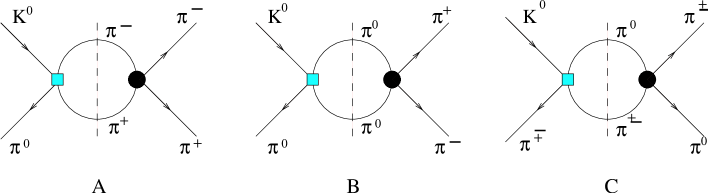
Figure 7: Diagrams for the calculation of FSI for $K_{L}\rightarrow\pi^{+}\pi^{-}\pi^{0}$ using the optical theorem. The square is the weak vertex and the circle is the strong one.

The calculation is analogous to the one for $K_{L}\rightarrow\pi^{0}\pi^{0}\pi^{0}$. The three contributions in Figure 7 correspond to two charged pions in the loop –results in Eqs. (99) and (103), two neutral pions in the loop –results in Eqs. (100) and (104)– and loops with one neutral and one charged pions. In the last case we have a S-wave contribution –results in (101) and (105), and a P wave contribution –results in (102) and (106), respectively. Eqs. (99), (100), (101), and (102) are the results of using the weak vertex at ${\cal{O}}(p^{4})$ and the strong vertex at ${\cal{O}}(p^{2})$. Eqs. (103), (104), (105), and (106) are the results of using the weak vertex at ${\cal{O}}(p^{2})$ and the strong vertex at ${\cal{O}}(p^{4})$.

$${\rm Im}A^{(6,1)}_{W} = \frac{\sigma(s_{3})}{16\pi f_{\pi}^{2}}(s_{3})\left[M_{1}(s_{3})+\widetilde{M}_{2}(s_{3})+\widetilde{M}_{3}(s_{3})(m_{K}^{2}+3m_{\pi}^{2}-2s_{3})\right.$$ (99)

$$\left.-\widetilde{M}_{3}^{s}(s_{3})\right]_{{\cal O}(p^{4})}\,,$$

$${\rm Im}A^{(6,2)}_{W} = \frac{\sigma(s_{3})}{32\pi f_{\pi}^{2}}(s_{3}-m_{\pi}^{2})\left[M_{0}(s_{3})+\widetilde{M}_{0}(s_{3})\right]_{{\cal O}(p^{4})}\,,$$ (100)

$${\rm Im}A^{(6,3)}_{W,S} = \frac{\sigma(s_{1})}{32\pi f_{\pi}^{2}}(m_{\pi}^{2}-s_{1}/2)\left[2M_{2}(s_{1})+\widetilde{M}_{2}(s_{1})+\widetilde{M}_{1}(s_{1})\right.$$ (101)

$$-\widetilde{M}_{3}(s_{1})(m_{K}^{2}+3m_{\pi}^{2}-2s_{1})\left.+\widetilde{M}_{3}^{s}(s_{1})\right]_{{\cal O}(p^{4})}+s_{1}\leftrightarrow s_{2}\,,$$

$${\rm Im}A^{(6,3)}_{W,P} = \frac{\sigma(s_{1})}{64\pi f_{\pi}^{2}}\frac{s_{1}(s_{2}-s_{3})}{s_{1}^{2}-2s_{1}(m_{K}^{2}+m_{\pi}^{2})+(m_{K}^{2}-m_{\pi}^{2})^{2}}$$ (102)

$$\times\left[(s_{1}-m_{K}^{2}-3m_{\pi}^{2})(\widetilde{M}_{2}(s_{1})-\widetilde{M}_{1}(s_{1})\right.$$

$$\left.+(2s_{1}-m_{K}^{2}-3m_{\pi}^{2})\widetilde{M}_{3}(s_{1}))+(2\widetilde{M}_{2}^{s}(s_{1})-2\widetilde{M}_{1}^{s}(s_{1})\right.$$

$$+\left.(5s_{1}-3m_{K}^{2}-9m_{\pi}^{2})\widetilde{M}_{3}^{s}(s_{1}))+2\widetilde{M}_{3}^{ss}(s_{1})+\frac{8}{3}b(s_{1})^{2}M_{3}(s_{1})\right]_{{\cal O}(p^{4})}$$

$$+s_{1}\leftrightarrow s_{2}\,.$$

$${\rm Im}A^{(6,1)}_{\pi} = \frac{\sigma(s_{3})}{16\pi}\left.(M_{1}(s_{3})+M_{3}(s_{3})(m_{K}^{2}+3m_{\pi}^{2}-3s_{3}))\right|_{p^{2}}\ (P_{5}(s_{3})+\widetilde{P}^{(0,0)}_{6}(s_{3}))\,,$$ (103)

$${\rm Im}A^{(6,2)}_{\pi} = \frac{\sigma(s_{3})}{32\pi}\left.(M_{0}(s_{3})+M_{0}(s_{1})+M_{0}(s_{2}))\right|_{p^{2}}\ (P_{3}(s_{3})+\widetilde{P}^{(0,0)}_{4}(s_{3}))\,,$$ (104)

$${\rm Im}A^{(6,3)}_{\pi,S} = \frac{\sigma(s_{1})}{32\pi}\left.\left(M_{1}(s_{1})+\frac{1}{2}M_{3}(s_{2})(s_{1}-s_{3})+\frac{1}{2}M_{3}(s_{3})(s_{1}-s_{2})\right)\right|_{p^{2}}$$ (105)

$$\times\Big{(}\widetilde{P}^{(0,0)}_{3}(s_{1})+\hat{P}^{(0)}_{1,4}(s_{1})+\widetilde{P}^{(0)}_{2,4}(s_{1})\Big{)}+s_{1}\leftrightarrow s_{2}$$

$${\rm Im}A^{(6,3)}_{\pi,P} = \frac{\sigma(s_{1})}{64\pi}\left.\left(3M_{3}(s_{1})(s_{2}-s_{3})\right)\right|_{p^{2}}\frac{1}{s_{1}-4m_{\pi}^{2}}$$ (106)

$$\!\!\!\times\Big{(}(s_{1}-4m_{\pi}^{2})(\widetilde{P}^{(0,0)}_{3}(s_{1})-\hat{P}^{(0)}_{1,4}(s_{1})+\widetilde{P}^{(0)}_{2,4}(s_{1}))+2\widetilde{P}^{(1,0)}_{3}(s_{1})$$

$$\!\!\!-2\widetilde{P}^{(1)}_{1,4}(s_{1})+2\hat{P}^{(1)}_{2,4}(s_{1})\Big{)}+s_{1}\leftrightarrow s_{2}\ .$$

B.4 FSI for $K_{S}\rightarrow\pi^{+}\pi^{-}\pi^{0}$ at NLO

The diagrams contributing to this decay are the same depicted in Figure 7. The result corresponding to diagram A in Figure 7 is in Eq. 107 for the weak vertex at ${\cal{O}}(p^{4})$ and the strong vertex at ${\cal{O}}(p^{2})$ and in Eq. B.4 for the weak vertex at ${\cal{O}}(p^{2})$ and the strong vertex at ${\cal{O}}(p^{4})$. In this case there is only P wave contribution.

Diagram B in Figure 7 does not contribute. Diagram C in Figure 7 gives both an S-wave – results in Eqs. (108) and (111)– and a P wave contribution – results in (109) and (112). Equations (108) and (109) are the results of the case in which the weak vertex is at ${\cal{O}}(p^{4})$ and strong vertex at ${\cal{O}}(p^{2})$ in diagram C. Equations (111) and (112) are the results for the case in which the weak vertex is at ${\cal{O}}(p^{2})$ and the strong vertex at ${\cal{O}}(p^{4})$ in diagram C.

$${\rm Im}A^{(6,1)}_{W,P} = \frac{\sigma(s_{3})}{16\pi f_{\pi}^{2}}\frac{s_{3}(s_{1}-s_{2})}{s_{3}^{2}-2(m_{K}^{2}+m_{\pi}^{2})s_{3}+(m_{K}^{2}-m_{\pi}^{2})^{2}}\left\{a(s_{3})(\widetilde{M}_{4}(s_{3})+(2a(s_{3})\right.$$ (107)

$$\!\!\!\left.-s_{3})\widetilde{M}_{5}(s_{3}))-(\widetilde{M}_{4}^{s}(s_{3})+(3a(s_{3})-s_{3})\widetilde{M}_{5}^{s}(s_{3}))+\widetilde{M}_{5}^{ss}(s_{3})\right.$$

$$\!\!\!\left.-\frac{2}{3}b(s_{3})^{2}M_{6}(s_{3})\right\}$$

$${\rm Im}A^{(6,2)}_{W,S} = \frac{\sigma(s_{1})}{64\pi f_{\pi}^{2}}(2m_{\pi}^{2}-s_{1})\left\{2M_{4}(s_{1})-\widetilde{M}_{4}(s_{1})+(m_{K}^{2}+3m_{\pi}^{2}-2s_{1})(\widetilde{M}_{5}(s_{1})\right.$$ (108)

$$\!\!\!\left.-\widetilde{M}_{6}(s_{1}))-\widetilde{M}_{5}^{s}(s_{1})+\widetilde{M}_{6}^{s}(s_{1})\right\}-s_{1}\leftrightarrow s_{2}\,,$$

$${\rm Im}A^{(6,2)}_{W,P} = \frac{\sigma(s_{1})}{32\pi f_{\pi}^{2}}\frac{s_{1}(s_{3}-s_{2})}{s_{1}^{2}-2s_{1}(m_{K}^{2}+m_{\pi}^{2})+(m_{K}^{2}-m_{\pi}^{2})}$$ (109)

$$\!\!\!\times\biggl{\{}\frac{4}{3}b(s_{1})^{2}M_{5}(s_{1})+a(s_{1})(\widetilde{M}_{4}(s_{1})-(2a(s_{1})-s_{1})(\widetilde{M}_{5}(s_{1})+\widetilde{M}_{6}(s_{1})))$$

$$\!\!\!-\widetilde{M}_{4}^{s}(s_{1})+(3a(s_{1})-s_{1})(\widetilde{M}_{5}^{s}(s_{1})+\widetilde{M}_{6}^{s}(s_{1}))-\widetilde{M}_{5}^{ss}(s_{1})-\widetilde{M}_{6}^{ss}(s_{1})\biggr{\}}$$

$$\!\!\!-s_{1}\leftrightarrow s_{2}$$

$${\rm Im}A^{(6,1)}_{\pi,P} = -\frac{\sigma(s_{3})}{16\pi}\frac{\left.(M_{4}(s_{1})-M_{4}(s_{2}))\right|_{p^{2}}}{s_{3}-4m_{\pi}^{2}}\left[(s_{3}-4m_{\pi}^{2})\widetilde{P}_{7}^{(0,0)}(s_{3})+2\widetilde{P}_{7}^{(0,1)}(s_{3})\right]\,,$$

$${\rm Im}A^{(6,2)}_{\pi,S} = \frac{\sigma(s_{1})}{64\pi}\left.M_{5}(s_{1})\right|_{p^{2}}(3s_{1}-(m_{K}^{2}+3m_{\pi}^{2}))(\widetilde{P}_{3}^{(0,0)}(s_{1})+\widetilde{P}_{2,4}^{(0)}(s_{1})$$ (111)

$$\!\!\!+\widetilde{P}_{1,4}^{(0)}(s_{1}))-s_{1}\leftrightarrow s_{2}\,,$$

$${\rm Im}A^{(6,2)}_{\pi,P} = \frac{\sigma(s_{1})}{64\pi}\left.\left(M_{4}(s_{2})-M_{4}(s_{3})\right)\right|_{p^{2}}\frac{1}{s_{1}-4m_{\pi}^{2}}$$ (112)

$$\!\!\!\times\Big{(}(s_{1}-4m_{\pi}^{2})(\widetilde{P}^{(0,0)}_{3}(s_{1})-\hat{P}^{(0)}_{1,4}(s_{1})+\widetilde{P}^{(0)}_{2,4}(s_{1}))+2\widetilde{P}^{(1,0)}_{3}(s_{1})$$

$$\!\!\!-2\widetilde{P}^{(1)}_{1,4}(s_{1})+2\hat{P}^{(1)}_{2,4}(s_{1})\Big{)}-s_{1}\leftrightarrow s_{2}\,.$$

Appendix C Three-Pion Cut Contributions to FSI Phases

To calculate the contributions of the topologies in Figure 1 C, D, and E to the FSI, we need the tree level vertices of $K\to 3\pi$ and $3\pi\to 3\pi$. The complete tree level amplitude of the $3\pi\to 3\pi$ scattering can be easily calculated using the code Ampcalculator developed in [24]. In this way all possible $3\pi\to 3\pi$ are included. In order to perform the integral in the phase space as prescribed in the optical theorem we assign the momentum to pions as shown in an example in Figure 8. The momentum assignment is done preserving the suffix $3$ for the odd pion in the $K^{+}\to 3\pi$ vertex.

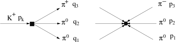
Figure 8: Example of diagram for the calculation of FSI for $K^{+}\to\pi^{0}\pi^{0}\pi^{+}$ with momentum assignment.

In order to perform the integral in the phase space over momentum $q_{i}$ it is necessary the fix a reference frame. We chose the reference frame in which the decaying kaon is at rest and the momentum $p_{3}$ defines the z-axis,

$$p_{K}=(M_{K},0,0,0),\quad p_{3}=(p_{3}^{0},0,0,\bar{p}_{3}),$$

$$p_{1}=(p_{1}^{0},0,\bar{p}_{1}\sin\eta,\bar{p}_{1}\cos\eta),\quad p_{2}=-p_{K}-p_{1}-p_{3}\ .$$ (113)

The momenta $q_{i}$ describe also a decay of a kaon into three pions. The most general expression for these momenta, in the chosen reference frame, is

$$q_{i} = R_{z}(\alpha)R_{y}(\beta)R_{z}(\gamma)\ r_{i}\ ,$$

$$r_{3}=(r_{3}^{0},0,0,\bar{r}_{3}),\quad r_{1} = (r_{1}^{0},0,\bar{r}_{1}\sin\theta,\bar{r}_{1}\cos\theta),\quad r_{2}=p_{K}-r_{1}-r_{3}\ ,$$ (114)

and $R_{z(y)}(\delta)$ are rotations around axis $z$ $(y)$ with Euler angle $\delta$. Using the Particle Data Group (PDG) parametrization for the phase space integrals [25], the LO contribution to $\mbox{Im}\overline{A}_{00+}$ and $\mbox{Im}\overline{B}_{00+}$ of the 3-pion cut diagrams so read

$$\mbox{Im}\overline{A}_{00+}^{3\pi,LO}(s_{1},s_{2},s_{3}) = \frac{1}{16(2\pi)^{5}}\int{\rm d}q_{3}^{0}\ {\rm d}q_{2}^{0}\ {\rm d}\alpha\ {\rm d}\cos\beta\ {\rm d}\gamma\left[A^{(p^{2})}_{00+}(p_{K},q_{i})A_{3\pi,0}^{(p^{2})}(q_{i},p_{i})\right]\ ,$$

$$v_{\pm}\mbox{Im}\overline{B}_{00+}^{3\pi,LO}(s_{1},s_{2},s_{3}) = \frac{1}{16(2\pi)^{5}}\int{\rm d}q_{3}^{0}\ {\rm d}q_{2}^{0}\ {\rm d}\alpha\ {\rm d}\cos\beta\ {\rm d}\gamma\left[A^{(p^{2})}_{++-}(p_{K},q_{i})A_{3\pi,\pm}^{(p^{2})}(q_{i},p_{i})\right]\ ,$$

where $A_{3\pi,0}^{(p^{2})}(q_{i},p_{i})$, $A_{3\pi,\pm}^{(p^{2})}(q_{i},p_{i})$ are the tree level amplitudes for $\pi^{0}\pi^{0}\pi^{+}\rightarrow\pi^{0}\pi^{0}\pi^{+}$ and $\pi^{+}\pi^{+}\pi^{-}\rightarrow\pi^{0}\pi^{0}\pi^{+}$. At this order the are no contribution of these topologies to $\mbox{Re}\overline{B}_{00+}$. We have computed numerically the integrals in (LABEL:eq:3p3pLO). The correction induced by (LABEL:eq:3p3pLO) to the other LO terms is always much below the $0.5\%$. We find so perfectly consistent to omit these corrections at this level of precision. Similar expressions and conclusions hold for the FSI in the decay of $K_{L}\rightarrow\pi^{0}\pi^{0}\pi^{0}$. For this case one just has

$$\mbox{Im}\overline{A}_{000}^{3\pi,LO}(s_{1},s_{2},s_{3}) = \frac{1}{16(2\pi)^{5}}\int{\rm d}q_{3}^{0}\ {\rm d}q_{2}^{0}\ {\rm d}\alpha\ {\rm d}\cos\beta\ {\rm d}\gamma\left[A^{(p^{2})}_{000}(p_{K},q_{i})\tilde{A}_{3\pi,0}^{(p^{2})}(q_{i},p_{i})\right]\ ,$$

$$v_{\pm}\mbox{Im}\overline{B}_{000}^{3\pi,LO}(s_{1},s_{2},s_{3}) = \frac{1}{16(2\pi)^{5}}\int{\rm d}q_{3}^{0}\ {\rm d}q_{2}^{0}\ {\rm d}\alpha\ {\rm d}\cos\beta\ {\rm d}\gamma\left[A^{(p^{2})}_{+-0}(p_{K},q_{i})\tilde{A}_{3\pi,\pm}^{(p^{2})}(q_{i},p_{i})\right]\ ,$$

where $\tilde{A}_{3\pi,0}^{(p^{2})}(q_{i},p_{i})$, $\tilde{A}_{3\pi,\pm}^{(p^{2})}(q_{i},p_{i})$ are the tree level amplitudes for $\pi^{0}\pi^{0}\pi^{0}\rightarrow\pi^{0}\pi^{0}\pi^{0}$ and $\pi^{+}\pi^{-}\pi^{0}\rightarrow\pi^{0}\pi^{0}\pi^{0}$.

References

- [1] G. Ecker, hep-ph/0011026; A. Pich, hep-ph/9806303.
- [2] G. Ecker, Prog. Part. Nucl. Phys. 35 (1995) 1; E. de Rafael, hep-ph/9502254; A. Pich, Rept. Prog. Phys. 58 (1995) 563.
- [3] S. Weinberg, Physica A 96 (1979) 327.
- [4] J. Gasser and H. Leutwyler, Annals Phys. 158 (1984) 142; Nucl. Phys. B 250 (1985) 465.
- [5] E. Gámiz, J. Prades and I. Scimemi, J. High Energy Phys. 10 (2003) 042; hep-ph/0410150; hep-ph/0305164.
- [6] I. Scimemi, E. Gámiz and J. Prades, Proc. of the Rencontres de Moriond on Electroweak Interactions and Unified Theories, p. 355, The Gioi Publishers (2005), hep-ph/0405204.
- [7] J. Prades, E. Gámiz and I. Scimemi, Proc. of QCD’05, Montpellier, 4-8 July 2005, hep-ph/0509346.
- [8] V. Bernard, N. Kaiser and U.-G. Meißner, Nucl. Phys. B 357 (1991) 129.
- [9] J. Bijnens, P. Dhonte and F. Persson, Nucl. Phys. B 648 (2003) 317.
- [10] J. Kambor, J. Missimer and D. Wyler, Nucl. Phys. B 346 (1990) 17; Phys. Lett. B 261 (1991) 496.
- [11] J. Kambor, J.F. Donoghue, B.R. Holstein, J. Missimer and D. Wyler, Phys. Rev. Lett. 68 (1992) 1818.
- [12] J. Bijnens and F. Borg, Nucl. Phys. B 697 (2004) 319; Eur. Phys. J. C 39 (2005) 347; A. Nehme, Phys. Rev. D 70 (2004) 094025.
- [13] J. Bijnens and F. Borg, Eur. Phys. J. C 40 (2005) 383.
- [14] N. Cabibbo, Phys. Rev. Lett. 93 (2004) 121801.
- [15] U.-G. Meißner, G. Müller and S. Steininger, Phys. Lett. B 406 (1997) 154 [Erratum-ibid. B 407 (1997) 454]; M. Knecht and R. Urech, Nucl. Phys. B 519 (1998) 329.
- [16] N. Cabibbo and G. Isidori, J. High Energy Phys. 03 (2005) 021.
- [17] G. D’Ambrosio, G. Isidori, A. Pugliese and N. Paver, Phys. Rev. D 50 (1994) 5767 [Erratum-ibid. D 51 (1995) 3975].
- [18] J.R. Batley et al. [NA48/2 Collaboration], Phys. Lett. B 633 (2006) 173; S. Giudici [NA48/2 Collaboration], hep-ex/0505032.
- [19] J. Gasser, Talk at IV EURIDICE Collaboration Meeting, Marseille 8-11 February 2006.
- [20] G. Colangelo, J. Gasser and H. Leutwyler, Phys. Lett. B 488 (2000) 261, Nucl. Phys. B 603 (2001) 125.
- [21] J.R. Peláez and F.J. Ynduráin, Phys. Rev. D 71 (2005) 074016; hep-ph/0412320.
- [22] J. Gasser, private communication; G. Colangelo, J. Gasser, B. Kubis, and A. Rusetsky, Phys. Lett. B 638 (2006) 187.
- [23] A.V. Anisovich, Phys. Atom. Nucl. 66 (2003) 172 [Yad. Fiz. 66 (2003) 175]; V.V. Anisovich and A.A. Ansel’m, Usp. Fiz. Nauk. 88 (1966) 287 [Sov. Phys. Usp. 9 (1966) 117].
- [24] R. Unterdorfer and G. Ecker, J. High Energy Phys. 10 (2005) 017.
- [25] S. Eidelman et al. [Particle Data Group], Phys. Lett. B 592 (2004) 1.