$Id:espcrc2.tex,v1.22004/02/2411:22:11speppingExp$ Automated Resummation and Hadron Collider Event Shapes Gavin P. Salam

Automated Resummation and Hadron Collider Event Shapes

Abstract

This writeup gives an introduction to the theoretical understanding that lies behind automated resummation. It then discusses its applications to hadron-collider event shapes.

The all-order resummation of logarithmically enhanced terms is essential for the detailed study of final-state observables like event shapes and jet rates (see for example [1]). The differential distribution for an event shape $V$ to have value $v$ can be written as

$$\frac{1}{\sigma}\frac{d\sigma}{dv}\equiv\Sigma^{\prime}(v)=\alpha_{s}f_{1}(v)+\alpha_{s}^{2}f_{2}(v)+\ldots$$ (1)

where the leading (LO) and next-to-leading (NLO) order coefficients $f_{1}$ and $f_{2}$ can be calculated with a program such as NLOJET [2]. At small $v$, for any observable sensitive to soft collinear radiation, the corresponding integrated distribution $\Sigma(v)$ has double-logarithmic enhancements at all orders

$$\Sigma(v) \simeq\sum_{m}\sum_{n=0}^{{2m}}H_{mn}\alpha_{s}^{m}\ln^{n}\frac{1}{v}\qquad(v\to 0)$$ (2a)

$$=\underbrace{h_{1}(\alpha_{s}L^{2})}_{LL_{{\Sigma}}}\,+\,\underbrace{\sqrt{\alpha_{s}}\,h_{2}(\alpha_{s}L^{2})}_{NLL_{{\Sigma}}}\,+\ldots$$ (2b)

where $H_{mn}$ are numerical coefficients and we have introduced the shorthand $L\equiv\ln 1/v$. The double logarithms are associated with non-cancellation between soft and collinear divergences in real and virtual graph, since limiting $v$ suppresses real radiation but not the corresponding virtual terms.

When $v$ is small ($\ln v\sim\alpha_{s}^{-1/2}$) all terms $\alpha_{s}^{m}L^{2m}$ become of the same magnitude ($\sim 1$) and reliable calculations for $\Sigma(v)$ can only be obtained by resumming these terms to all orders, giving the leading logarithmic (LL) function $h_{1}(\alpha_{s}L^{2})$. One can systematically reorganise the whole perturbative series in terms of the logarithmic enhancements, eq. (2b), with next-to-leading logarithmic (NLL) terms, $\alpha_{s}^{m}L^{2m-1}$ resummed into a function $\sqrt{\alpha_{s}}h_{2}(\alpha_{s}L^{2})$, etc., such that each of the $h_{n}$ is of order $1$.

For yet smaller $v$, $L\gg\alpha_{s}^{-1/2}$, even the reorganisation of eq. (2) breaks down, since the functions $h_{n}$ can themselves become large as their argument, $\alpha_{s}L^{2}$, grows beyond $1$. It turns out however that quite often eq. (2) can be written as the exponential of a much less divergent series,

$$\ln\Sigma(v) \simeq\sum_{m}\sum_{n=0}^{{m+1}}G_{mn}\alpha_{s}^{m}L^{n}\qquad(v\to 0)$$ (3a)

$$=\underbrace{Lg_{1}(\alpha_{s}L)}_{LL_{{\ln\Sigma}}}\,+\,\underbrace{g_{2}(\alpha_{s}L)}_{NLL_{{\ln\Sigma}}}\,+\ldots\,,$$ (3b)

where the key feature of eq. (3a) is that the index $n$ now runs only up to $m+1$, i.e. all the double logarithms of $\Sigma$ arise from the exponentiation of a single $\alpha_{s}L^{2}$ term in $\ln\Sigma$. This series can be also reorganised systematically, eq. (3b) and now one redefines the LL terms to be $Lg_{1}(\alpha_{s}L)$ and the NLL to be $g_{2}(\alpha_{s}L)$, etc., where the $g_{n}(\alpha_{s}L)$ have the property that they are all of order $1$ as long as $L\sim\alpha_{s}^{-1}$. This means that the reorganised perturbative hierarchy remains stable to much smaller values of $v$, than in eq. (2); furthermore the NLL terms are more suppressed with respect to the LL terms (by $1/L\sim\alpha_{s}$) than was the case in the classification of eq. (2b).

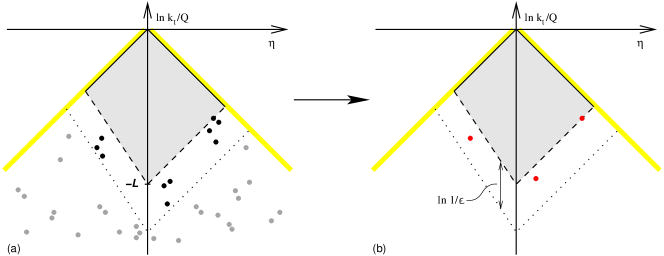
Figure 1: Representation of phase space in $e^{+}e^{-}\to 2$ jets; emissions (points) in the right (left) hand half-plane are collinear to the right (left) hand jet. For further details, see text.

In this writeup it is the more ambitious, exponentiated, kind of resummation that will be discussed. Let us examine the kinematic plane in $e^{+}e^{-}$, fig. 1, represented in terms of the transverse momentum $k_{t}$ and rapidity ($\eta=\frac{1}{2}\frac{E+k_{z}}{E-k_{z}}$) of an emission $k$, as measured with respect to the Born $q\bar{q}$ axis. The thick yellow lines represent the hard-collinear kinematic limit for emissions. If there is just a single emission, one calculates the ${\cal O}\left(\alpha_{s}\right)$ term of the logarithmically enhanced part of $\Sigma(v)$ by identifying the grey shaded area in which the observable’s value $V(k)$ is larger than $v$. In the single-emission approximation this region is forbidden to real radiation, but not to virtual corrections, and the resulting non-cancellation leads to a double logarithmic contribution $\alpha_{s}L^{2}$ to $\Sigma(V)$.

In general, when considering multiple emissions, the boundary $V(k_{1},\ldots,k_{n})<v$ will be a complex multi-dimensional function of the $k_{i}$. For many observables there are several simplifications that can be carried out. These will look quite similar to those, based on infrared and collinear (IRC) safety, that are used to justify fixed-order calculations. We use as a reference scale the lower boundary (dashed line) of the shaded region in fig. 1a, corresponding to a value $\sim v=e^{-L}$ of the observable for a single emission. Regardless of the set of emissions that is present, we require that all emissions much softer than the scale of the boundary should modify the observable by much less than $v$. These emissions (in grey, below the dotted line) can therefore be neglected, since they will cancel fully against corresponding virtual terms. Then, only the remaining, black emissions, between the dashed and dotted lines, will contribute significantly to the observable. These are clustered in rapidity since there is a collinear divergence for the splitting of an emitted parton. However, most common observables have the property that they are insensitive to this collinear splitting, so that each cluster of black emissions can be replaced by a single red ‘primary’ emission, as shown in fig. 1b.

For the next stage, it is necessary to exploit another property common to most observables, namely that

$$V(k_{1},\ldots,k_{n})\sim\max[V(k_{1}),\ldots,V(k_{n})]\,,$$ (4)

so that if $V(k_{1},\ldots,k_{n})<v$ then all $V(k_{i})\lesssim v$. This means that the shaded region will contain no emissions (except potentially near its lower edge) implying a resummation of purely virtual corrections there. This leads to the exponentiated double logarithmic contribution $Lg_{1}(\alpha_{s}L)$.

What remains to be calculated is the correction coming from real emissions, confined to the band (approximately) between the shaded and dotted lines. As long as the observable is such that one can ensure that this band has a width $\ln 1/\epsilon$ that is not parametrically large (i.e. independent of $L$), then the band will give at most single-logarithmic contributions $\alpha_{s}^{n}L^{n}$, i.e. it will contribute only to the $g_{2}(\alpha_{s}L)$ function, not to $g_{1}$. Because the density of primary emissions per unit rapidity in the band, $\sim\alpha_{s}\ln 1/\epsilon$ will be low, emissions will be widely separated in rapidity, allowing one to make use of the property of angular ordering whereby the full matrix element for multiple emission reduces to that for independent emission [3], simplifying the calculation of $g_{2}$. Note that this only works for continuously global observables [4, 5].

To aid the mathematical treatment of the above procedures it is convenient to parametrise the observable’s dependence on a single emission close to hard leg $\ell$ (in $e^{+}e^{-}\to 2$ jets, $\ell=1,2$) as

$$V(k)=d_{\ell}g_{\ell}(\phi)\left(\frac{k_{t}}{Q}\right)^{a}e^{-b_{\ell}\eta}\,,$$ (5)

with $k_{t}$ and $\eta$ now measured with respect to leg $\ell$, and $a$, $b_{\ell}$ and $d_{\ell}$ numerical constants and $g_{\ell}(\phi)$ a function of the azimuthal angle $\phi$, all of them characteristic of the observable and relevant to determining the position of the dashed line in fig.1 for a given $v$ (where $\phi$ is not represented). One also defines $\bar{d}_{\ell}=d_{\ell}\exp\,[\,\int_{0}^{2\pi}\!\frac{d\phi}{2\pi}\ln g_{\ell}(\phi)]$.

It will be useful to express momenta in terms of the effect they have on the observable, through functions $\kappa_{i}(\zeta)$ that satisfy

$$V(\kappa_{i}(\zeta))=\zeta\,.$$ (6)

This condition alone is not enough to fully specify $\kappa_{i}(\zeta)$ — additionally one needs to know the leg $\ell_{i}$ to which it is collinear, its azimuthal angle $\phi_{i}$, and how its rapidity depends on $\zeta$ — for concreteness here we will take this to be $\eta_{i}(\zeta)=\xi_{i}(\ln 1/\zeta)/(a+b_{\ell})$ so that taking $\xi_{i}$ in the range $0<\xi_{i}<1$, $\kappa_{i}(\zeta)$ will span from the large-angle soft region to the hard-collinear region (regardless of $\zeta$).

Part of the logic of this scaling is that the emission pattern $\sim\alpha_{s}\frac{dk_{t}}{k_{t}}d\eta$ becomes proportional to $\alpha_{s}L\cdot d\ln\zeta d\xi$, with the single logarithmic factor $\alpha_{s}L$ factoring out explicitly. It also helps compactify conditions such as eq. (4), which becomes

$$V(\kappa_{1}(\zeta_{1}),\ldots,\kappa_{n}(\zeta_{n}))\sim\max(\zeta_{1},\ldots\zeta_{n})\,.$$ (7)

Actually “$\sim$” is difficult to encode directly in a computer, as will be needed for automation. Here the meaning of “$\sim$” is that the ratio between the two sides should not be parametrically large, even if one scales all the $\zeta_{i}$ by a common large factor (i.e. no new large ratios should appear in the problem, because they could lead to large logarithms). This suggests the following more precise condition,

$$\lim_{\bar{v}\to 0}\frac{V(\kappa_{1}(\bar{v}\zeta_{1}),\ldots,\kappa_{n}(\bar{v}\zeta_{n}))}{\bar{v}}=f_{\{\kappa_{i}\}}(\zeta_{1},\ldots,\zeta_{n})\,,$$ (8)

where $f_{\{\kappa_{i}\}}$ should be some well-defined non-zero function and where the subscript indicates that it may depend also on the additional characteristics of the $\kappa_{i}$ ($\ell_{i}$, $\xi_{i}$, $\phi_{i}$).

The $\kappa_{i}$ are also useful in formulating the precise conditions needed to go from fig.1a to fig.1b. For example we needed the observable to be such that we could neglect the grey emissions, leaving only those in the band between the dashed and dotted lines — furthermore we needed to be able to require that the width of the band, $\ln 1/\epsilon$, was not parametrically large, i.e. would not be associated with extra logarithms. This is equivalent to saying that in eq. (8), independently of $\bar{v}$ on the left-hand-side, there should exist an $\epsilon$ such that any emissions with $\zeta_{i}<\epsilon$ can be neglected, or

$$\lim_{\zeta_{n}\to 0}f_{\{\kappa_{i}\}}(\zeta_{1},\ldots,\zeta_{n})=f_{\{\kappa_{i}\}}(\zeta_{1},\ldots,\zeta_{n-1})\,.$$ (9)

This looks very much like infrared safety, but is stronger because $f_{\{\kappa_{i}\}}$ already involves an infrared limit of its own. Accordingly we call it recursive infrared safety. Making use simultaneously of normal infrared safety it can also be rewritten in terms of a commutator of limits,

$$\left[\lim_{\zeta_{n}\to 0},\lim_{\bar{v}\to 0}\right]\frac{V(\kappa_{1}(\bar{v}\zeta_{1}),\ldots,\kappa_{n}(\bar{v}\zeta_{n}))}{\bar{v}}=0\,.$$ (10)

Similarly, to ensure that one can replace the clusters of black emission in fig.1a with single emissions in fig.1b, one needs a condition called recursive collinear safety.

Given these recursive IRC (rIRC) conditions, exponentiation is guaranteed, and to NLL accuracy one has

$$\ln\Sigma_{V}(v)=L{\cal G}_{1}(\alpha_{s}L,a,\{b_{\ell}\})+\\ +{\cal G}_{2}(\alpha_{s}L,a,\{b_{\ell}\},\{\bar{d}_{\ell}\})+{\cal F}_{V}(R^{\prime})\,,$$ (11)

where the ${\cal G}_{i}$ are known analytical functions whose observable dependence enters only through the $a$, $b_{\ell}$ and $\bar{d}_{\ell}$ coefficients; $R^{\prime}=\partial_{L}(L{\cal G}_{1}(\alpha_{s}L,a,\{b_{\ell}\}))$ and the NLL ${\cal F}_{V}(R^{\prime})$ accounts for the observable’s non-trivial dependence on multiple emissions. In most cases it is given by

$${\cal F}_{V}(R^{\prime})=\lim_{\epsilon\to 0}\frac{\epsilon^{R^{\prime}}}{R^{\prime}}\sum_{m=0}^{\infty}\frac{1}{m!}\times\\ \times\left(\prod_{i=1}^{m+1}\sum_{\ell_{i}=1}^{n}R_{\ell_{i}}^{\prime}\int_{\epsilon}^{1}\frac{d\zeta_{i}}{\zeta_{i}}\int_{0}^{2\pi}\frac{d\phi_{i}}{2\pi}\right)\delta\!\left(\ln\zeta_{1}\right)\times\\ \times\exp\left(-R^{\prime}\ln f_{\{\kappa_{i}\}}(\zeta_{1},\ldots,\zeta_{m+1})\right)\,.$$ (12)

where $R_{\ell_{i}}^{\prime}$ is the contribution to $R^{\prime}$ from leg $\ell$.

Resummation is automated through an expert system (CAESAR [6]) which uses high precision arithmetic to (a) probe the observable in the soft and collinear region to obtain the $a$, $b_{\ell}$ and $d_{\ell}$ coefficients and the $g_{\ell}(\phi)$, (b) test the rIRC safety, (c) evaluate ${\cal F}_{V}(R^{\prime})$ via Monte Carlo integration.

One of the most non-trivial applications of CAESAR is to dijet event shapes at proton-(anti)proton colliders. Such event shapes are of interest for various reasons, among them sensitivity to a new class of soft colour-evolution anomalous dimensions [7], and the prospect of extracting information about non-perturbative correction from gluon hadronisation and from the underlying event. Unfortunately the event shapes measured so far [8] are not global and therefore not within the scope of CAESAR. Globalness is a significant issue at hadron-colliders because detectors are not able to measure the whole event, but only up to some limited maximum rapidity, $\eta_{\max}\simeq 3.5$ at the Tevatron ($\sim 5$ for LHC).

There are two main ways of working around this problem. Firstly one can define an event shape that measures everywhere (directly global) [9], and then note that if $\eta_{\max}$ is sufficiently large, then the error introduced by actually measuring only particles with $|\eta|<\eta_{\max}$ is of order $\delta V={\bar{d}}_{i}e^{-(a+b_{i})\eta_{\max}},$ where $b_{i}$, $\bar{d}_{i}$ are the $b_{\ell}$, $\bar{d}_{\ell}$ coefficients for the incoming hadron legs. As long as most of the event shape distribution is concentrated at values of the observable much larger than this, then the non-measurement of particles with $|\eta|>\eta_{\max}$ has a negligible impact on the distribution.

Table 1: Properties of the various event shapes proposed in [10]. Entries marked with an asterisk are subject to uncertainties.

Event-shape	Impact of $\eta_{\max}$	Resummation breakdown	Underlying Event	Jet hadronisation
$\tau_{\perp,g}$	tolerable∗	none	$\sim\eta_{\max}/Q$	$\sim 1/Q$
$T_{m,g}$	tolerable	none	$\sim\eta_{\max}/Q$	$\sim 1/(\sqrt{\alpha_{s}}Q)$
$y_{23}$	tolerable	none	$\sim\sqrt{y_{23}}/Q^{*}$	$\sim\sqrt{y_{23}}/Q\,^{*}$
$\tau_{\perp,{\cal E}}$, $\rho_{X,{\cal E}}$	negligible	none	$\sim 1/Q$	$\sim 1/Q$
$B_{X,{\cal E}}$	negligible	none	$\sim 1/Q$	$\sim 1/(\sqrt{\alpha_{s}}Q)$
$T_{m,{\cal E}}$	negligible	serious	$\sim 1/Q$	$\sim 1/(\sqrt{\alpha_{s}}Q)$
$y_{23,{\cal E}}$	negligible	none	$\sim 1/Q$	$\sim\sqrt{y_{23}}/Q\,^{*}$
$\tau_{\perp,{\cal R}}$, $\rho_{X,{\cal R}}$	none	serious	$\sim 1/Q$	$\sim 1/Q$
$T_{m,{\cal R}}$, $B_{X,{\cal R}}$	none	tolerable	$\sim 1/Q$	$\sim 1/(\sqrt{\alpha_{s}}Q)$
$y_{23,{\cal R}}$	none	intermediate∗	$\sim\sqrt{y_{23}}/Q\,^{*}$	$\sim\sqrt{y_{23}}/Q\,^{*}$

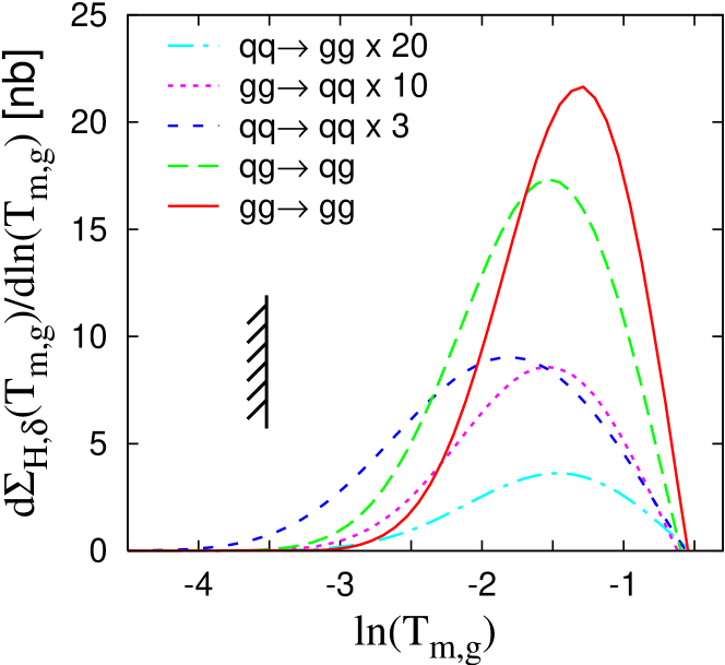
Figure 2: Resummed distribution of $T_{m,g}$ for Tevatron events where the hardest jet has $E_{\perp}>50\,\mathrm{GeV}$. The point where the $\eta_{\max}=3.5$ cutoff becomes relevant is indicated by a hashed line.

Among these directly-global observables, there are two subclasses. Firstly there are those naturally defined in the whole event, a transverse thrust $\tau_{\perp,g}$, its minor $T_{m,g}$ and the resolution parameter at which the $k_{t}$ jet-finder goes from classifying an event as $2+2$-jet like to $3+2$-jet like, $y_{23}$. The resummed distribution for $T_{m,g}$ is shown in fig. 2.

Alternatively one can define a main event shape in a central region $\cal C$ (e.g. $|\eta|<1$) and add to it an exponentially-suppressed contribution for particles in the forward region ${\cal E}_{\cal\bar{C}}=\sum_{i\not\in\cal C}k_{ti}/Q_{\perp,\cal C}e^{-|\eta_{i}-\eta_{\cal C}|},$ where $Q_{\perp,\cal C}$ is the sum of transverse momenta of particles in $\cal C$ and $\eta_{\cal C}$ is the (transverse-momentum weighted) mean rapidity of particles in $\cal C$. Such ‘combined’ observables can be constructed starting from the ‘naturally global’ event shapes given above, and also from event shapes that only make sense when defined in the central region such as jet broadenings and invariant masses, giving e.g. $B_{T,{\cal E}}$. The naturally global observables always have $b_{i}=0$ and are more sensitive to the $\eta_{\max}$ cut (cf. fig. 2) than those combined with the forward exponential suppression, which have $b_{i}=a$.

One can also define ‘indirectly-global’ observables. Here too there is a main event shape in the central region and to it one adds a recoil term ${\cal R}_{\perp\cal C}=\left|\sum_{i\in\cal C}{\vec{k}}_{ti}\right|/Q_{\perp,\cal C}$ measured in $\cal C$, which through momentum-conservation is sensitive to emissions outside $\cal C$. This eliminates the problem of sensitivity to $\eta_{\max}$, however instead one runs into the issue that the CAESAR resummation is reliable only as long as the main mechanism by which an observable can take a small value is by suppression of radiation. If instead it can have a small value through cancellations between different emissions (as with a vector recoil) then the resummation breaks down via a divergence of ${\cal F}(R^{\prime})$ at some small but finite value of $v$.

Table 1 summarises the impact of $\eta_{\max}$ and resummation breakdown (if any) for a range of observables defined in [10]. It is gives expectations for the degree of sensitivity to the underlying event and jet hadronisation, illustrating the complementarity between observables.

The work presented here was carried out in collaboration with A. Banfi and G. Zanderighi. I wish to thank the organisers of the RADCOR 2005 Symposium for the welcoming and stimulating atmosphere of the conference as well as for financial support.

References

- [1] M. Dasgupta and G. P. Salam, J. Phys. G 30 (2004) R143.
- [2] Z. Nagy, Phys. Rev. Lett. 88, 122003 (2002) and references therein.
- [3] S. Catani et al., Nucl. Phys. B 407, 3 (1993).
- [4] M. Dasgupta and G. P. Salam, Phys. Lett. B 512, 323 (2001); JHEP 0203 (2002) 017
- [5] M. Dasgupta and G. P. Salam, JHEP 0208, 032 (2002).
- [6] A. Banfi, G. P. Salam and G. Zanderighi, Phys. Lett. B 584 (2004) 298; JHEP 0503 (2005) 073.
- [7] J. Botts and G. Sterman, Nucl. Phys. B 325, 62 (1989); N. Kidonakis and G. Sterman, Phys. Lett. B 387 (1996) 867; N. Kidonakis, G. Oderda and G. Sterman, Nucl. Phys. B 531, 365 (1998); R. Bonciani et al., Phys. Lett. B 575 (2003) 268.
- [8] F. Abe et al. [CDF Collaboration], Phys. Rev. D 44 (1991) 601; I. A. Bertram [D0 Collaboration], Acta Phys. Polon. B 33, 3141 (2002).
- [9] A. Banfi et al., JHEP 0111, 066 (2001).
- [10] A. Banfi, G. P. Salam and G. Zanderighi, JHEP 0408 (2004) 062.