Construction and analysis of a simplified many-body neutrino model

Abstract

In dense neutrino systems, such as found in the early Universe, or near a supernova core, neutrino flavor evolution is affected by coherent neutrino-neutrino scattering. It has been recently suggested that many-particle quantum entanglement effects may play an essential role in these systems, potentially invalidating the traditional description in terms of a set of single-particle evolution equations. We model the neutrino system by a system of interacting spins, following an earlier work which showed that such a spin system can in some cases be solved exactly Friedland_&_Lunardini_1 . We extend this work by constructing an exact analytical solution to a more general spin system, including initial states with asymmetric spin distribution and, moreover, not necessarily aligned along the same axis. Our solution exhibits a rich set of behaviors, including coherent oscillations and dephasing and a transition from the classical to quantum regimes. We argue that the classical evolution of the spin system captures the entire coherent behavior of the neutrino system, while the quantum effects in the spin system capture some, but not all, of the neutrino incoherent evolution. By comparing the spin and neutrino systems, we find no evidence for the violation of the accepted one-body description, though the argument involves some subtleties not appreciated before. The analysis in this paper may apply to other two-state systems beyond the neutrino field.

I Introduction

In many neutrino systems that are currently studied the rate of incoherent interactions is low enough to be completely negligible, yet coherent interactions (refraction) play an important, even crucial role. A classical example is provided by the case of solar neutrinos: these neutrinos hardly scatter inside the Sun; nevertheless, their coherent interactions with the solar matter plays an essential role in their flavor evolution. This is of course the celebrated MSW theory of neutrino oscillations in matter Wolfenstein ; MS .

The classical MSW theory describes neutrino propagation in a background of normal matter (electrons, neutrons, protons). There are systems, however, where the number density of neutrinos themselves exceeds those of electrons and baryons, such as the early universe, or the so-called hot bubble region in an exploding supernova. Such systems additionally require a theory describing neutrino self-refraction.

Early investigations treated the neutrino background analogously to the MSW theory Fuller ; Notzold . Pantaleone Pantaleone1992prd ; Pantaleone1992plb , McKellar and Thomson McKellar_Thomson , and Sigl and Raffelt Sigl_Raffelt showed, however, that the neutrino background is distinguished by an important subtlety: the induced mass terms in general have nonzero off-diagonal components in the flavor basis. Physically, this means that flavor can be coherently exchanged between the neutrinos.

The authors of McKellar_Thomson ; Pantaleone1992prd ; Pantaleone1992plb ; Sigl_Raffelt constructed the equation of motion of the neutrino system by using a one-body description for each neutrino. This treatment crucially depends on the assumption that the state of the system can be factorized into a product of one-particle states. If this is not the case and the wavefunctions of individual neutrinos are entangled, a very different treatment may be required. A priori, it is not obvious that neutrinos would not develop such entanglement, due to the off-diagonal induced mass terms. So the question arises whether this entanglement exists and has a substantial impact on the coherent flavor evolution of the neutrino ensemble. The answer could have a significant impact on the predictions for the supernova neutrino signal, the synthesis of heavy elements in the supernova, and possibly Big Bang Nucleosynthesis and cosmology.

The question was recently examined by Friedland & Lunardini (F&L I Friedland_&_Lunardini_2 , F&L II Friedland_&_Lunardini_1 ) and by Bell, Rawlinson and Sawyer (BRS Bell ). All three papers used a similar setup, with a Hamiltonian that was restricted to “forward scattering” only Pantaleone1992plb . While F&L I argued that the coherent part of the neutrino evolution should be described by the one-particle formalism, the BRS paper reached an opposite conclusion.

To make their argument, BRS considered the evolution of a system initially in the flavor eigenstates. With this choice, the one-particle formalism predicts no coherent flavor conversion and thus conversion on the coherent time scale in this system would be an indication of the breakdown of the one-particle description (presumably through the formation of many-neutrino entangled states). The numerical calculation performed by BRS seemed to suggest the presence of such “fast” conversions, although the calculations involved a relatively small numbers of neutrinos.

F&L II Friedland_&_Lunardini_1 subsequently solved the neutrino model introduced by BRS analytically for the special case of equal numbers of each neutrino species and equal strength interactions by mapping neutrino-neutrino interactions to spin-spin interactions. The solution in the limit of many particles exhibited the equilibration time that is precisely what would be expected from incoherent scattering. The analytical solution thus supported the one-particle description of the system.

One may wonder, however, if the initial state considered in F&L II, namely, equal numbers of spins “up” and “down” was somehow special. Could entanglement appears with a more general setup?

In this paper we will present a generalization of the many-body neutrino model introduced in F&L II, in the hope of understanding the quantum system better. We again consider a system of many neutrinos in which there are two flavor species, so that it maps to a system of interacting spins (thanks to the $SU(2)$ symmetry of the problem). We generalize the model to initial states in which the species are not equally populated and where the initial states are not necessarily in flavor eigenstates. We show that the corresponding spin problem can still be solved exactly. The resulting solution exhibits a rich set of behaviors, as will be discussed in the following.

Even generalized in this way, the model still involves several simplifications and it is important to spell these out.

• The model keeps only forward scattering terms. Thus, while the model should correctly capture coherent effects in a real neutrino system, conclusions about incoherent scattering effects in our model must be interpreted with care.

• The momentum degrees of freedom are ignored. The effects of Fermi statistics are not included, that is the physical neutrino system is assumed to have a phase-space density much less than one. This is indeed satisfied everywhere outside the neutrinosphere in a supernova. The case of the neutrinos in the early universe may be more subtle .

• The interaction strength between any two neutrinos is taken to be the same, ignoring the angular distribution of the neutrino momenta (see later). The model thus aims to describe the physical situation in an isotropic neutrino gas and hence may or may not capture all effects that could arise as a result of very anisotropic momentum distributions, such as those suggested in Sawyer2004 ; Sawyer2005 .

These limitations and assumptions should be kept in mind when relating the results obtained for the spin system to the behavior of a real neutrino gas.

The problem of the flavor evolution in dense neutrino systems continues to receive a significant amount of attention. In addition to the above mentioned papers Friedland_&_Lunardini_2 ; Bell ; Friedland_&_Lunardini_1 ; Sawyer2004 ; Sawyer2005 , the reader is referred to Boyanovsky:2004xz ; Sirera:2004rv ; Strack:2005ux ; Strack:2005jj ; Ho:2005vj ; DuanFuller2005 for recent progress.

II Setup and Goals

II.1 The Hamiltonian and Eigenvalues

We follow Bell and Friedland_&_Lunardini_1 by considering a system consisting of interacting massless neutrinos represented by plane waves in a box of volume $V$. Since our primary motivation is to investigate coherent effects in the neutrino system, in particular, the possible breakdown of the one-body approximation due to flavor exchange, and not due to spatially dependent many-body correlations, we focus on the “forward” neutral current interactions between the neutrinos. In other words, we drop the momentum degrees of freedom and include only scattering events that preserve neutrino momenta and those that exchange the momenta Pantaleone1992plb ; Friedland_&_Lunardini_2 ,

$$|\nu_{x}(\vec{k})\nu_{y}(\vec{p})\rangle \longrightarrow |\nu_{x}(\vec{k})\nu_{y}(\vec{p})\rangle,$$ (1)

$$|\nu_{x}(\vec{k})\nu_{y}(\vec{p})\rangle \longrightarrow |\nu_{x}(\vec{p})\nu_{y}(\vec{k})\rangle.$$ (2)

In the “usual” case of electrons, protons and neutrons in the background, the waves scattered forward interfere coherently. For the neutrino background, however, this is not necessarily so and our model, in addition to coherent effects, captures some of the incoherent effects as well Friedland_&_Lunardini_2 ; Friedland_&_Lunardini_1 . The identification of coherent and incoherent effects will be discussed at length in what follows.

For $E_{\nu}\ll m_{Z^{0}}$ the neutral current interaction Hamiltonian is

$$H_{int}=\frac{G_{F}}{\sqrt{2}}\left(\sum_{\alpha}\bar{\nu}_{\alpha}\gamma^{\mu}\nu_{\alpha}\right)\left(\sum_{\beta}\bar{\nu}_{\beta}\gamma_{\mu}\nu_{\beta}\right).$$ (3)

Here the sum is over all $k$ flavors. The Hamiltonian is invariant under a flavor $SU(k)$ symmetry. Let us consider only two neutrino species, in which case the symmetry becomes $SU(2)$ and the flavor space structure of the $\nu-\nu$ interaction becomes equivalent to the interaction between pairs of spins. As explicitly shown in F&L II, the interaction energy of two neutrinos, 1 and 2, is proportional to the square of the total angular momentum of the corresponding spin system,

$$\hat{L}^{2}\equiv(\vec{\sigma}_{1}/2+\vec{\sigma}_{2}/2)^{2}=(3/2+\vec{\sigma}_{1}\cdot\vec{\sigma}_{2}/2).$$ (4)

The coefficient of proportionality dependents on the relative angle between the neutrino momenta $\Theta$, $g=\frac{\sqrt{2}G_{F}}{V}(1-\cos\Theta)$ Pantaleone1992plb . In a realistic neutrino system, the couplings are distributed according to the distribution of the relative angles between neutrino momenta. In order to make our system solvable, we will simplify the problem and take all the couplings to be the same

$$g=\frac{\sqrt{2}G_{F}}{V}.$$ (5)

It is hoped that this simplification preserves the essential features of the evolution Bell ; Friedland_&_Lunardini_1 (see, however, Sawyer2004 ; Sawyer2005 ). Henceforth we study this system of interacting spins to obtain information about the neutrino system.

We will consider a system of $N+M$ spins, such that initially $N$ spins all have a certain orientation (for definiteness, without a loss of generality, “up”) and the remaining $M$ spins all have a certain different orientation. At $t=0$, thus, the $N$ spins combine in a state of angular momentum $J_{N}=N/2$ and projection $m_{N}=N/2$, and the M spins in a state of angular momenta $J_{M}=M/2$ and projection $m_{M}$. In terms of the original neutrino system, we have a system of $N$ electron neutrinos, $|\nu_{e}\rangle$, and $M$ neutrinos in some other state $|\nu_{x}\rangle$. We give the answer for a general $|\nu_{x}\rangle$ and then explicitly study two cases: $|\nu_{x}\rangle$ is flavor eigenstate $|\nu_{\mu}\rangle$ and $|\nu_{x}\rangle$ is a flavor superposition state $(|\nu_{e}\rangle+|\nu_{\mu}\rangle)/\sqrt{2}$.

The Hamiltonian for this system is

$$H=g\sum_{j=1}^{N+M-1}\sum_{k=j+1}^{N+M}(\vec{\sigma}_{j}+\vec{\sigma}_{k})^{2}=g\left(\sum_{j=1}^{N+M-1}\sum_{k=j+1}^{N+M}2\vec{\sigma}_{j}\cdot\vec{\sigma}_{k}+\frac{3}{4}(N+M)(N+M-1)\right).$$ (6)

which is related to the square of the total angular momentum of the system Friedland_&_Lunardini_1 ,

$$\hat{J}^{2} = \left(\sum_{j=1}^{N+M}\vec{\sigma}_{j}\right)^{2}$$ (7)

$$= \left(\sum_{j=1}^{N+M-1}\sum_{k=j+1}^{N+M}2\vec{\sigma}_{j}\cdot\vec{\sigma}_{k}+\frac{3}{4}(N+M)\right).$$

By comparing Eqs. (6) and (7) we find

$$H_{int}=g[\hat{J}^{2}+\frac{3}{4}(M+N)(M+N-2)],$$ (8)

with eigenvalues

$$E(J,N,M)= g\left[J(J+1)+\frac{3(M+N)(M+N-2)}{4}\right],$$ (9)

where

$$J_{\rm min} \leq J\leq J_{\rm max},$$ (10)

$$J_{\rm min} = {\rm max}(|m_{N}-m_{M}|,|N/2-M/2|),$$ (11)

$$J_{\rm max} = N/2+M/2.$$ (12)

II.2 Goals

We are interested in finding the probability, as a function of time, $P_{1}(t)$, of one of the particles remaining in the “spin up” state if it was initially in the “spin up” state. As discussed in Friedland_&_Lunardini_1 , the time scale with which this probability evolves, $t_{\rm eq}$, tells us whether the evolution has coherent or incoherent nature. In particular, for $M=N$,

$$t_{\rm eq}^{coh} \sim (gN)^{-1},$$ (13)

$$t_{\rm eq}^{inc} \sim (g\sqrt{N})^{-1},$$ (14)

for coherent and incoherent evolution correspondingly. In a large spin system the coherent time scale is much shorter then the incoherent one. One of our goals will be to see which timescales are present in our solution under different initial conditions.

The second goal is to compare the coherent evolution we find to the predictions of the one-particle formalism. According to this formalism, the coherent evolution of a given neutrino is determined by the following one-particle Hamiltonian Pantaleone1992plb ; Pantaleone1992prd :

$$H_{1-part}=\frac{\sqrt{2}G_{F}}{V}\sum_{i}|\psi_{i}\rangle\langle\psi_{i}|.$$ (15)

Here, $\psi_{i}$ is the flavor state of the $i$th “background” neutrino i.e. the background is all the neutrinos except for the one for which the equation is written. Explicitly, for two neutrino species ($\nu_{e}$ and $\nu_{\mu}$) $|\psi_{i}\rangle=\left[\begin{array}[]{c}\nu_{e}^{i}\\ \nu_{\mu}^{i}\end{array}\right]$. The sum runs over all “background” neutrinos.

III The Probability of Spin Preservation

III.1 Result

As we show in this Section, the evolution of our system can be solved exactly. In the interests of clarity, we begin by displaying the answer for $P_{1}(t)$:

$$P_{1}(t) = \frac{1}{2}+\sum_{J=J_{\rm min}}^{J_{\rm max}}C(J)$$ (16)

$$+ \sum_{J=J_{\rm min}}^{J_{\rm max}-1}\eta(J)\ \cos[gt(2J+2)].$$

The first two terms in Eq. (16) give the mean value of the probability: $P_{1}=1/2$ means complete depolarization, or in the language of the neutrino system, an equal incoherent mixture of the two flavors; the second term thus given the degree of polarization of the mean (“equilibrated”) state. The last term contains the time evolution of the system.

The limits of the summation $J_{\rm min}$ and $J_{\rm max}$ are given in Eq. (11) and (12). The coefficients $C(J)$ and $\eta(J)$ given by

$$C(J) = (-1)^{2J-(m_{N}+m_{M})+(N+M)/2+1}(1+2J)\frac{1}{N}\sqrt{(N/2)(N/2+1)(N+1)}$$ (19)

$$\times |\langle N/2,m_{N},M/2,m_{M}|J,m_{N}+m_{M}\rangle|^{2}$$

$$\times \begin{pmatrix}J&1&J\\ -(m_{N}+m_{M})&0&m_{N}+m_{M}\end{pmatrix}\left\{\begin{array}[]{ccc}N/2&J&M/2\\ J&N/2&1\end{array}\right\},$$

$$\eta(J) = (-1)^{2J-(m_{N}+m_{M})+(N+M)/2}\sqrt{(1+2J)(3+2J)}\frac{2}{N}\sqrt{(N/2)(N/2+1)(N+1)}$$ (22)

$$\times \langle N/2,m_{N},M/2,m_{M}|J,m_{N}+m_{M}\rangle\langle N/2,m_{N},M/2,m_{M}|J+1,m_{N}+m_{M}\rangle$$

$$\times \begin{pmatrix}J+1&1&J\\ -(m_{N}+m_{M})&0&m_{N}+m_{M}\end{pmatrix}\left\{\begin{array}[]{ccc}N/2&J+1&M/2\\ J&N/2&1\end{array}\right\}.$$

The inner products in the last two equations are Clebsch-Gordan coefficients, the objects in the parentheses are $3j$-coefficients and those in curly brackets are $6j$-coefficients. For definitions, see, e.g., Landavshitz .

The rest of this Section presents two complementary derivations of these results. The derivations are somewhat technical and the reader primarily interested in the analysis of the rich physical properties of the solution may wish to skip to Sect. IV and return to this Section later, as needed.

III.2 Construction of the probability: overview

This solution can be found in either of two ways, both of which provide important, complementary physical insights into the spin system. These insights will prove very useful later, as we discuss the physical properties of the solution. Additionally, one or the other method may be useful for addressing still more general spin configurations. Correspondingly, we show both methods.

• The first approach is to “split off” the first spin from the system, so that the remaining $N+M-1$ spins forms “a background” it interacts with. The solution is constructed by first coupling the angular momenta of the remaining spins and then coupling the first spin to the result. This method generalizes the idea employed in Friedland_&_Lunardini_1 , but without relying on the symmetries specific to the $N=M$ case.

• The second approach is to treat the first spin as a part of the system. We solve for the evolution of all spins that start out in the “up” state. The solution can be found by observing that even with $N\neq M$ the system possesses a very high degree of symmetry: all spins that start out in the same state evolve in the same way. This means, as we will show, that the problem can be reduced to that of just two coupled angular momenta.

III.3 Method I: splitting off the first spin

The outline of this approach is as follows. The time evolution of the system is easily written down in the basis of total angular momentum, since, as explained in Sect. II, this is the Hamiltonian eigenbasis. Correspondingly, we begin in Sect. III.3.1 by constructing the density matrix for the system in this basis. In Sect. III.3.2, this density matrix is rotated to a basis in which the first spin has a well-defined value. Finally, in Sect. III.3.3 the probability $P_{1}(t)$ is found.

III.3.1 Constructing the many-body density matrix in the total angular momentum basis

Our system begins (at time $t=0$) in the state

$$S(0)=|\thickspace j_{N},m_{N}\thickspace\rangle\otimes|\thickspace j_{M},m_{M}\thickspace\rangle.$$ (23)

Recall $j_{N}=N/2$ is the total angular momentum of all the spin up particles, each with angular momentum $\frac{1}{2}$, and projection along the $\hat{z}$ direction, $m_{N}$. Also, $j_{M}=M/2$ is the angular momentum of all the background particles, each with angular momentum $\frac{1}{2}$ and projection, $m_{M}$. Rotating the initial state, Eq.(23), to the total angular momentum ($J$) basis and evolving it to time $t$, we have,

$$S(t)=\sum_{J=J_{\rm min}}^{J_{\rm max}} \langle\thickspace j_{N},j_{M},J,m\thickspace|\thickspace j_{N},j_{M},m_{N},m_{M}\thickspace\rangle$$ (24)

$$\times e^{-itE(J,N,M)}\thickspace|\thickspace j_{N},j_{M},J,m\thickspace\rangle.$$

Here $\langle\thickspace j_{N},j_{M},J,m\thickspace|\thickspace j_{N},j_{M},m_{N},m_{M}\thickspace\rangle$ is the Clebsch-Gordan coefficient where $j_{N}$ and $j_{M}$ are coupled to the total angular momentum of the system $J$ with projection in the $\hat{z}$ direction of $m=m_{N}+m_{M}$.

The density matrix is defined as

$$\rho(t)=|\thickspace S(t)\thickspace\rangle\langle\thickspace S(t)\thickspace|.$$ (25)

Hence we have,

$$\rho(t) =\sum_{J=J_{\rm min}}^{J_{\rm max}}\sum_{J^{\prime}=J_{\rm min}}^{J_{\rm max}} e^{-it\Delta E(J,J^{\prime})}\langle\thickspace j_{N},j_{M},J,m\thickspace|\thickspace j_{N},j_{M},m_{N},m_{M}\thickspace\rangle\langle\thickspace j_{N},j_{M},J^{\prime},m\thickspace|\thickspace j_{N},j_{M},m_{N},m_{M}\thickspace\rangle$$ (26)

$$\thickspace|\thickspace j_{N},j_{M},J,m\thickspace\rangle\langle\thickspace j_{N},j_{M},J^{\prime},m\thickspace|.$$

Here $\Delta E(J,J^{\prime})=g[J(J+1)-J^{\prime}(J^{\prime}+1)]$ is the difference between the eigenvalues $E(J,N,M)$ and $E(J^{\prime},N,M)$.

III.3.2 Construction of the density matrix in the basis $|\frac{1}{2},\lambda\rangle\otimes|j,\mu\rangle$

Figure 1: Graphical representation of recoupling. The diagram on the left represents the original coupling: the net angular momentum ($j_{1}$) of the $N$ spins pointing up and the net angular momentum ($j_{2}$) of the remaining $M$ spins are coupled to the total angular momentum of the system ($J$). The diagram on the right represents the new coupling (see main text for description). $k$ is the momentum of $N-1$ “up” spins.

To find the probability of spin preservation it is convenient to again change the basis, this time to $|\frac{1}{2},\lambda\rangle\otimes|j,\mu\rangle$. $\quad|\frac{1}{2},\lambda\rangle$ is the state of one of the spin-1/2 particles with projection $\lambda$ and $|j,\mu\rangle$ is the state of $M+N-1$ remaining particles with angular momenta j and projection $\mu$. The density matrix in the new basis is constructed in this subsection and then the probability is found in the next subsection. We start with the state of Eq. (24), and transform it to the new basis. We will omit the limits on the summation signs for the next few equations but will comment on these later.

To change to the preferred basis ($|\frac{1}{2},\lambda\rangle\otimes|j,\mu\rangle$) we modify how the angular momenta couple to the total angular momentum, $J$. This can be done in any way that is convenient. We for the moment “remove” the first spin up and combine the $N-1$ spins up (with net angular momentum $k=j_{N}-1/2$) and the remaining $M$ spins (with net angular momentum $j_{M}$) into an object with angular momentum $j$. We then couple the removed spin and $j$ to the total $J$. Therefore $j$ is the result of coupling $j_{M}$ and $k$. See Fig. 1 for a pictorial interpretation.

The state $|\thickspace j_{N},j_{M},J,m\thickspace\rangle$ is represented in the new basis as

$$|\thickspace j_{N},j_{M},J,m\thickspace\rangle = \sum_{j}\langle\thickspace\frac{1}{2},(k\thickspace j_{M})j;J\thickspace|\thickspace(\frac{1}{2}\thickspace k)j_{N},j_{M};J\thickspace\rangle$$ (27)

$$\times \thickspace|\thickspace\frac{1}{2},(k\thickspace j_{M})j;J,m\thickspace\rangle.$$

The notation $(a\thickspace b)c$ indicates that $a$ and $b$ couple to $c$. Here the recoupling coefficient $\langle\thickspace\frac{1}{2},(k\thickspace j_{M})j;J\thickspace|\thickspace(\frac{1}{2}\thickspace k)j_{N},j_{M};J\thickspace\rangle$ is proportional to the 6-j coefficient,

$$\langle\thickspace\frac{1}{2},(k\thickspace j_{M})j;J\thickspace|\thickspace(\frac{1}{2}\thickspace k)j_{N},j_{M};J\thickspace\rangle\equiv(-1)^{\frac{1}{2}+k+J+j_{M}}\left[(2j_{N}+1)(2j+1)\right]^{\frac{1}{2}}\left\{\begin{array}[]{ccc}\frac{1}{2}&k&j_{N}\\ j_{M}&J&j\\ \end{array}\right\}.$$ (28)

For a definition and explanation of 6-j coefficients see Brink or Landavshitz , Eq. (108.6). The right side of this coefficient represents the original coupling (the left side of Fig. 1). The left side represents the changed coupling (the right side of Fig. 1). The 6-j coefficient is a consequence of changing the coupling.

Rotating from the basis $\thickspace|\thickspace\frac{1}{2},(k\thickspace j_{M})j;J,m\thickspace\rangle$ to the basis $|\thickspace\frac{1}{2},\lambda\thickspace\rangle\otimes|\thickspace j,\mu\thickspace\rangle$ and substituting $k=j_{N}-1/2$, we have,

$$\begin{split}|\thickspace j_{N},j_{M},J,m\thickspace\rangle=&\sum_{j,\lambda,\mu}(-1)^{J+j_{M}+j_{N}}\left[(2j_{N}+1)(2j+1)\right]^{\frac{1}{2}}\langle\thickspace\frac{1}{2},j,\lambda,\mu\thickspace|\thickspace\frac{1}{2},j;J,m\thickspace\rangle\\ &\times\left\{\begin{array}[]{ccc}\frac{1}{2}&j_{N}-\frac{1}{2}&j_{N}\\ j_{M}&J&j\\ \end{array}\right\}\thickspace|\thickspace\frac{1}{2},\lambda\thickspace\rangle\otimes\thickspace|\thickspace j,\mu\thickspace\rangle.\end{split}$$ (29)

Finally, substituting Eq. (29) into Eq. (24) yields

$$S(t) = \sum_{J,j,\lambda,\mu}(-1)^{J+j_{M}+j_{N}}\left[(2j_{N}+1)(2j+1)\right]^{\frac{1}{2}}e^{-itE(J,N,M)}\langle\thickspace j_{N},j_{M},J,m\thickspace|\thickspace j_{N},j_{M},m_{N},m_{M}\thickspace\rangle$$ (32)

$$\times \langle\thickspace\frac{1}{2},j,\lambda,\mu\thickspace|\thickspace\frac{1}{2},j;J,m\thickspace\rangle\left\{\begin{array}[]{ccc}\frac{1}{2}&j_{N}-\frac{1}{2}&j_{N}\\ j_{M}&J&j\\ \end{array}\right\}\thickspace|\thickspace\frac{1}{2},\lambda\thickspace\rangle\otimes\thickspace|\thickspace j,\mu\thickspace\rangle.$$

Recall that the first $N$ spins are initially in a state with total angular momentum $j_{N}=N/2$. The initial state of the test spin is consequently the same as that of the other $N-1$ particles, “up” ($\lambda=+1/2$).

It is now simple to construct the density matrix in this new basis using Eq. (32) and $\rho=|\thickspace S(t)\thickspace\rangle\langle\thickspace S(t)\thickspace|$. We present the density matrix in component form,

$$\begin{split}\rho_{\frac{1}{2}\thickspace\lambda,\thickspace j\thickspace\mu\thickspace;\thickspace\frac{1}{2}\thickspace\lambda^{\prime},\thickspace j^{\prime}\thickspace\mu^{\prime}}(t)=\sum_{J,J^{\prime}}&e^{-it\Delta E(J,J^{\prime})}(-1)^{J-J^{\prime}}(2j_{N}+1)(2j+1)\langle\thickspace j_{N},j_{M},J,m\thickspace|\thickspace j_{N},j_{M},m_{N},m_{M}\thickspace\rangle\\ &\times\langle\thickspace j_{N},j_{M},J^{\prime},m\thickspace|\thickspace j_{N},j_{M},m_{N},m_{M}\thickspace\rangle\langle\thickspace\frac{1}{2},j,\lambda,\mu\thickspace|\thickspace\frac{1}{2},j;J,m\thickspace\rangle\\ &\times\langle\thickspace\frac{1}{2},j^{\prime},\lambda^{\prime},\mu^{\prime}\thickspace|\thickspace\frac{1}{2},j^{\prime};J^{\prime},m\thickspace\rangle\left\{\begin{array}[]{ccc}\frac{1}{2}&j_{N}-\frac{1}{2}&j_{N}\\ j_{M}&J&j\\ \end{array}\right\}\left\{\begin{array}[]{ccc}\frac{1}{2}&j_{N}-\frac{1}{2}&j_{N}\\ j_{M}&J^{\prime}&j^{\prime}\\ \end{array}\right\}.\end{split}$$ (33)

III.3.3 Probability of Spin Preservation

The probability that the first spin remains in the up state can be found from the density matrix. In general the probability of an eigenvalue $a_{i}$ represented by the operator A is $\mbox{Tr}(A\rho)$. In this case the operator is diagonal and hence probabilities are just the diagonal components of the density matrix. These components of the density matrix which give probabilities are those where $j=j^{\prime}$, $\mu=\mu^{\prime}$, and $\lambda=\lambda^{\prime}$, i.e., $\rho_{\frac{1}{2}\thickspace\lambda,\thickspace j\thickspace\mu;\frac{1}{2}\thickspace\lambda,\thickspace j\thickspace\mu}$. Furthermore we are looking for the probability of the first spin remaining in the spin up state so that $\lambda=+\frac{1}{2}$. Using this information together with Eq. (33) we find the probability to be

$$P_{1}(t) = \sum_{j,\mu}\rho_{\frac{1}{2}\thickspace\frac{1}{2},\thickspace j\thickspace\mu;\frac{1}{2}\thickspace\frac{1}{2},\thickspace j\thickspace\mu}=\sum_{J,J^{\prime},j,\mu}e^{-it\Delta E(J,J^{\prime})}(-1)^{J-J^{\prime}}(2j_{N}+1)(2j+1)\langle\thickspace j_{N},j_{M},J,m\thickspace|\thickspace j_{N},j_{M},m_{N},m_{M}\thickspace\rangle$$ (38)

$$\times \langle\thickspace j_{N},j_{M},J^{\prime},m\thickspace|\thickspace j_{N},j_{M},m_{N},m_{M}\thickspace\rangle\langle\thickspace\frac{1}{2},j,\frac{1}{2},\mu\thickspace|\thickspace\frac{1}{2},j;J,m\thickspace\rangle\langle\thickspace\frac{1}{2},j,\frac{1}{2},\mu^{\prime}\thickspace|\thickspace\frac{1}{2},j;J^{\prime},m\thickspace\rangle$$

$$\times \left\{\begin{array}[]{ccc}\frac{1}{2}&j_{N}-\frac{1}{2}&j_{N}\\ j_{M}&J&j\\ \end{array}\right\}\left\{\begin{array}[]{ccc}\frac{1}{2}&j_{N}-\frac{1}{2}&j_{N}\\ j_{M}&J^{\prime}&j\\ \end{array}\right\}.$$

The third Clebsch-Gordan coefficient in Eq. (38), $\langle\thickspace\frac{1}{2},j,\frac{1}{2},\mu\thickspace|\thickspace\frac{1}{2},j;J,m\thickspace\rangle$, represents the coupling of $\frac{1}{2}$ and $j$ to $J$. This gives $J-\frac{1}{2}\leqslant j\leqslant J+\frac{1}{2}$. In this same Clebsch-Gordan notice that we must have $\frac{1}{2}+\mu=m$, so that the summation over $\mu$ is unnecessary. Analyzing the fourth Clebsch-Gordan coefficient, $\langle\thickspace\frac{1}{2},j,\frac{1}{2},\mu^{\prime}\thickspace|\thickspace\frac{1}{2},j;J^{\prime},m\thickspace\rangle$, further simplifies the equation. This coefficient shows that we couple $\frac{1}{2}$ and $j$ to $J^{\prime}$. Hence we have, $|j-\frac{1}{2}|\leqslant J^{\prime}\leqslant j+\frac{1}{2}$. Now if $j=J+\frac{1}{2}$ then $J\leqslant J^{\prime}\leqslant J+1$, and if $j=J-\frac{1}{2}$ then $|J-1|\leqslant J^{\prime}\leqslant J$. Therefore $J^{\prime}=|J-1|,J,J+1$.

Summing over $J^{\prime}$ we find

$$\begin{split}P_{1}(t)&=\sum_{J=J_{\rm min}}^{J_{\rm max}}\tilde{C}(J)\\ &+\sum_{J=J_{\rm min}}^{J_{\rm max}-1}\eta(J)\cos[t\Delta E(J+1,J)],\end{split}$$ (39)

where

$$\begin{split}\tilde{C}(J)&=\sum_{j=J-\frac{1}{2}}^{J+\frac{1}{2}}(2j_{N}+1)(2j+1)\\ &\times\left|\langle\thickspace j_{N},j_{M},J,m\thickspace|\thickspace j_{N},j_{M},m_{N},m_{M}\thickspace\rangle\right|^{2}\\ &\times\left|\langle\thickspace\frac{1}{2},j,\frac{1}{2},m-\frac{1}{2}\thickspace|\thickspace\frac{1}{2},j;J,m\thickspace\rangle\right|^{2}\\ &\times\left|\left\{\begin{array}[]{ccc}\frac{1}{2}&j_{N}-\frac{1}{2}&j_{N}\\ j_{M}&J&j\\ \end{array}\right\}\right|^{2}\end{split}$$ (40)

and

$$\begin{split}\eta(J)&=-2(2j_{N}+1)(2J+2)\\ &\times\langle\thickspace j_{N},j_{M},J,m\thickspace|\thickspace j_{N},j_{M},m_{N},m_{M}\thickspace\rangle\\ &\times\langle\thickspace j_{N},j_{M},J+1,m\thickspace|\thickspace j_{N},j_{M},m_{N},m_{M}\thickspace\rangle\\ &\times\langle\thickspace\frac{1}{2},J+\frac{1}{2},\frac{1}{2},m-\frac{1}{2}\thickspace|\thickspace\frac{1}{2},J+\frac{1}{2};J,m\thickspace\rangle\\ &\times\langle\thickspace\frac{1}{2},J+\frac{1}{2},\frac{1}{2},m-\frac{1}{2}\thickspace|\thickspace\frac{1}{2},J+\frac{1}{2};J+1,m\thickspace\rangle\\ &\times\left\{\begin{array}[]{ccc}\frac{1}{2}&j_{N}-\frac{1}{2}&j_{N}\\ j_{M}&J&J+\frac{1}{2}\\ \end{array}\right\}\left\{\begin{array}[]{ccc}\frac{1}{2}&j_{N}-\frac{1}{2}&j_{N}\\ j_{M}&J+1&J+\frac{1}{2}\\ \end{array}\right\}.\end{split}$$ (41)

Although it is not immediately obvious, the answer just obtained coincides with Eqs. (16), (19), and (22). Notice that $\tilde{C}(J)$ is not the same as $C(J)$ in Eq. (19) since, unlike Eq. (16), Eq. (39) does not contain the 1/2 term.

III.4 Method II: symmetry of the entire system

The second method is based on an observation that since the coupling strength is the same for all spins the system possesses a very high degree of symmetry. In particular, all spins that start out in the same state evolve in the same way (up to relabeling). This simple observation proves to be very powerful for our analysis: it means that all spins that start out in the “up” state combine in a single composite object with the angular momentum $L_{1}=N/2$ at any moment in time, not just at $t=0$. The same can be said about the remaining $M$ spins ($L_{2}=M/2$). Thus the problem reduces to a textbook case of just two interacting angular momenta.

More precisely, at any moment in time, the system is described as a superposition of states $i$ with definite values of total angular momentum, $J_{i}$. Each such state is obtained as a result of symmetrizations and antisymmetrizations of individual spin wavefunctions. The highest $J$ state is a completely symmetrical combination, the next one is obtained by performing one antisymmetrization, etc (the general rules are given by Young’s tableaux). The important point is that by symmetry all spins that started out in the same state can only be symmetrized. That means that all spins that started out in the same state can be assembled in a single object with the total (unchanging in time!) angular momentum. This argument holds for any $t$.

It is conceptually straightforward to compute the expectation value of the operator $j_{z}^{(1)}$ (the $z$ component of the angular momentum of the first composite object) at any moment in time. The expectation value of the corresponding operator for each spin, $s_{z}^{(1)}$, can then be found by simply dividing by $N$, by symmetry.

Let us denote the state of the whole system by $|S(t)\rangle$. As before, the system evolves according to

$$|S(t)\rangle=\sum_{J=J_{\rm min}}^{J_{\rm max}}|J\rangle\langle J|S(0)\rangle e^{-itE_{J}},$$ (42)

where $J_{min}$ and $J_{max}$ are given in Eqs. (11) and (12), $E_{J}\equiv E(J,N,M))$ given in Eq. (9) (the irrelevant constant piece can be dropped).

We need to find the probability of the first spin being in the “up” state, $P_{1}(t)=\langle S(t)|+1/2\rangle_{1}\langle+1/2|_{1}|S(t)\rangle$. It follows from the definition of $s_{z}^{(1)}=1/2(|+1/2\rangle\langle+1/2|-|-1/2\rangle\langle-1/2|)$ and the completeness relation $(|+1/2\rangle\langle+1/2|+|-1/2\rangle\langle-1/2|=1)$ that this probability is related to the expectation value of the angular momentum of that spin,

$$P_{1}(t)=\langle S(t)|s_{z}^{(1)}|S(t)\rangle+1/2.$$ (43)

Let us now compute $\langle S(t)|s_{z}^{(1)}|S(t)\rangle$:

$$\langle S(t)|s_{z}^{(1)}|S(t)\rangle=\frac{1}{N}\langle S(t)|j_{z}^{(1)}|S(t)\rangle=\frac{1}{N}\sum_{J=J_{\rm min}}^{J_{\rm max}}\sum_{J^{\prime}=J_{\rm min}}^{J_{\rm max}}\langle S(0)|J^{\prime}\rangle\langle J^{\prime}|j_{z}^{(1)}|J\rangle\langle J|S(0)\rangle e^{it(E_{J}-E_{J^{\prime}})}.$$ (44)

The products $\langle J|S(0)\rangle$, $\langle S(0)|J^{\prime}\rangle$ are just the Clebsch-Gordan coefficients $\langle N/2,m_{N},M/2,m_{M},|J,m_{N}+m_{M}\rangle$, $\langle N/2,m_{N},M/2,m_{M},|J^{\prime},m_{N}+m_{M}\rangle$ (written so because they are real). The problem of finding the expectation value $\langle J^{\prime}|j_{z}^{(1)}|J\rangle$ is solved, e.g., in Landavshitz . Using Eqs. (109.2), (109.3), (29.13) there, and the fact that the operator $j_{z}^{(1)}$ is a $q=0$ component of a $k=1$ spherical tensor (see (107.1) of Landavshitz for the exact definition), we get

$$\langle J^{\prime}|j_{z}^{(1)}|J\rangle = \begin{pmatrix}J^{\prime}&1&J\\ -(m_{N}+m_{M})&0&m_{N}+m_{M}\end{pmatrix}$$

$$\times \sqrt{(1+2J)(1+2J^{\prime})}\left\{\begin{array}[]{ccc}N/2&J^{\prime}&M/2\\ J&N/2&1\end{array}\right\}$$

$$\times \sqrt{(N/2)(N/2+1)(N+1)}$$

$$\times (-1)^{q},$$ (48)

where

$$q \equiv max[J,J^{\prime}]-(m_{N}+m_{N})+N/2+M/2$$ (49)

$$+ min[J,J^{\prime}]+1.$$

The first line in Eq. (III.4) expresses the dependence of the matrix element on the $z$-component of the angular momentum of the whole system (Eq. (109.2) of Landavshitz ). The second line contains the dependence of the reduced matrix element on the total angular momenta $J$ and $J^{\prime}$ (Eq. (109.3) of Landavshitz ). The third line is the reduced matrix element of the angular momentum of the first composite object, $\langle j^{(1)}|j^{(1)}|j^{(1)}\rangle=\sqrt{L_{1}(L_{1}+1)(1+2L_{1})}$. Finally, the last line contains the sign factor collected from all the ingredients.

The 6j-symbol enforces the following selection rule:

$$J^{\prime}=J,J\pm 1.$$ (50)

The double sum in Eq. (44) then reduces to

$$\langle S(t)|s_{z}^{(1)}|S(t)\rangle=$$

$$\frac{1}{N}\sum_{J=J_{\rm min}}^{J_{\rm max}}|\langle N/2,m_{N},M/2,m_{M},|J,m_{N}+m_{M}\rangle|^{2}$$

$$\times \begin{pmatrix}J&1&J\\ -(m_{N}+m_{M})&0&m_{N}+m_{M}\end{pmatrix}$$

$$\times (1+2J)\left\{\begin{array}[]{ccc}N/2&J&M/2\\ J&N/2&1\end{array}\right\}$$

$$\times \sqrt{(N/2)(N/2+1)(N+1)}$$

$$\times (-1)^{2J-(m_{N}+m_{N})+N/2+M/2+1}$$

$$+ \frac{1}{N}\sum_{J=J_{\rm min}}^{J_{\rm max}-1}\langle N/2,m_{N},M/2,m_{M},|J,m_{N}+m_{M}\rangle$$

$$\times \langle N/2,m_{N},M/2,m_{M},|J+1,m_{N}+m_{M}\rangle$$

$$\times \begin{pmatrix}J+1&1&J\\ -(m_{N}+m_{M})&0&m_{N}+m_{M}\end{pmatrix}$$

$$\times \sqrt{(1+2J)(3+2J)}\left\{\begin{array}[]{ccc}N/2&J+1&M/2\\ J&N/2&1\end{array}\right\}$$

$$\times \sqrt{(N/2)(N/2+1)(N+1)}$$

$$\times (-1)^{2J-(m_{N}+m_{N})+N/2+M/2}$$

$$\times 2\cos[2gt(J+1)],$$ (57)

which is the answer given earlier in Eqs. (16), (19), and (22).

IV Analysis: a flavor superposition background

As already mentioned, the solution in Eqs. (16), (19), and (22) contains very rich physics found in the actual neutrino system. First, let us show that it contains both coherent oscillations and incoherent equilibration (decay). For that, let us consider the case

$$m_{N}=\frac{N}{2},\hskip 8.5359ptm_{M}=0.$$ (58)

In the neutrino system, this corresponds to the first $N$ neutrinos initially being in the $|\nu_{e}\rangle$ flavor eigenstate, while the remaining $M$ neutrinos starting out in the maximally mixed state. In this setup, the one-particle formalism predicts coherent evolution.

Figure 2: Time evolution of $P_{1}(t)$ in the case $N=100$, $M=120$, $m_{N}=N/2$, $m_{M}=0$. The time variable is defined as $\tau\equiv gt(M+N)$.

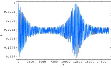
Indeed, our solution confirms this. The explicit form of the coefficients $C(J)$ and $\eta(J)$ is given in Eqs. (92) and (93). Using these values, we plot the behavior of the expectation value $P_{1}(t)$ for $N=100$, $M=120$ in Fig. 2. We see that the evolution exhibits both oscillations and decay. The oscillations reflect coherent behavior, while the decay occurs on a longer time scale, as would be expected for incoherent evolution.

This assertion can be made quantitative. The key test of coherence/incoherence of the evolution is the scaling of the evolution times with the number of particles. In the limit of large $N$ and $M$, it is possible to show that a single “wavetrain” in Fig. 2 (oscillations plus decay) is described analytically by the following formula:

$$P_{1}(t) = \frac{1}{2}\left(1+\frac{N^{2}}{N^{2}+M^{2}}\right)$$ (59)

$$+ \frac{1}{2}\left(1-\frac{N^{2}}{N^{2}+M^{2}}\right)\exp\left[-\frac{g^{2}t^{2}}{\frac{2}{N}+2\frac{N}{M^{2}}}\right]$$

$$\times \cos\left(g\sqrt{N^{2}+M^{2}}t\right).$$

A detailed derivation of Eq. (59) is given in Appendix B. Here, we notice that the oscillation period scales as $\propto(N^{2}+M^{2})^{-1/2}$, as expected for coherent evolution, while the decay time goes like $N^{-1/2}(2+2N^{2}/M^{2})^{1/2}$, indicating its incoherent nature (cf Eqs. (13), (14)).

We further observe that the frequency of the coherent oscillations agrees with the predictions of the one-particle formalism for a neutrino in the background of $M$ maximally neutrinos $(|\nu_{e}\rangle+|\nu_{\mu}\rangle)/\sqrt{2}$ and $N-1\simeq N$ neutrinos in the $|\nu_{e}\rangle$ state. Indeed, the one-particle oscillation Hamiltonian (15) in this case is

$$H_{1-part}=\frac{\sqrt{2}G_{F}}{V}\sum_{i}|\psi_{i}\rangle\langle\psi_{i}|=g\begin{pmatrix}N+\frac{M}{2}&\frac{M}{2}\\ \frac{M}{2}&\frac{M}{2}\end{pmatrix},$$ (60)

so that the oscillation frequency, given by the difference of the eigenvalues, is precisely $g\sqrt{N^{2}+M^{2}}$.

A very valuable physical insight can be gained from the idea that underlies Method II of solving for the evolution of the system, namely, that all spins in the same initial state always combine to form an object with a certain definite value of the angular momentum. As explained in Sect. (III.4), this means that the system can be reduced to just two coupled angular momenta, $j_{N}=N/2$ and $j_{M}=M/2$. When the numbers of spins $N$ and $M$ are sufficiently large, the two composite angular momenta behave as nearly classical objects. They precess about the direction of the total angular momentum of the system. These are the fast oscillations seen in Fig. 2.

Quantum-mechanically, a system that has a definite value of the total angular momentum does not simultaneously have definite projections of the individual angular momentum vectors that comprise it. Correspondingly, after a while the components of the angular momenta that are transverse to the total angular momentum undergo “quantum wash-out”. The system equilibrates to a state in which only the components of the constituent angular momenta along the direction of the total angular momentum remain.

Let us check this quantitatively. The total angular momentum of the system (in the classical limit) makes an angle $\cos\alpha=N/\sqrt{N^{2}+M^{2}}$ with the positive $z$ direction. Hence, the projection of the net angular momentum of the first $N$ spins on the direction of the total angular momentum of the whole system is $N/2\times\cos\alpha$. After a sufficient amount of time this is the only component that remains, the transverse components are washed-out. Projecting it back on the $z$-axis, we get $N/2\times\cos^{2}\alpha$ or, using Eqs. (43), (44),

$$\bar{P}_{1}=\frac{1}{2}+\frac{1}{N}\frac{N}{2}\frac{N^{2}}{N^{2}+M^{2}}=\frac{1}{2}\left(1+\frac{N^{2}}{N^{2}+M^{2}}\right),$$ (61)

precisely in agreement with Eq. (59).

Additional insight about classical and quantum features of the evolution can be gained by restoring the factors of the Plank’s constant in Eq. (59). It is simple to see that the product $gt$ comes with a one factor of $\hbar$. The logic is as follows: (i) from Eq. (9) it is obvious that the energy is proportional to $\hbar^{2}$ (from the angular momentum squared factor); (ii) next, in computing the evolution phase ($\exp(iEt/\hbar)$), we divide by one power of $\hbar$; (iii) this leads to one power of $\hbar$ in the argument of the cosine in Eq. (14), i.e., $gt$ comes with one factor of $\hbar$. Eq. (59) then reads

$$P_{1}(t) = \frac{1}{2}\left(1+\frac{N^{2}}{N^{2}+M^{2}}\right)$$ (62)

$$+ \frac{1}{2}\left(1-\frac{N^{2}}{N^{2}+M^{2}}\right)\exp\left[-g^{2}\hbar t^{2}\frac{M\hbar}{2\left(\frac{M}{N}+\frac{N}{M}\right)}\right]$$

$$\times \cos\left(g\hbar\sqrt{N^{2}+M^{2}}t\right).$$

We see that the argument of the cosine $g\hbar\sqrt{N^{2}+M^{2}}t=gJ_{\rm tot}t$ involves only the classical value of the total angular momentum $J_{\rm tot}$, while the decay exponent involves two powers of $\hbar$, of which only one is absorbed into the definition of classical angular momenta. The decay exponent is a quantum effect, in a sense that its physical origin lies in the quantum uncertainty principle. This allows us to make an important identification: coherent evolution in the neutrino system maps into the classical behavior of the angular momenta, while incoherent effects in the neutrino system correspond to quantum effects in the spin system. This important point will be developed further in Sect. V.1.

Finally, we note that the solution is periodic and the wavetrain, having seemingly completely decayed away, reemerges after some time. This phenomenon is due to the fact that the spin system possesses a fundamental frequency, of which all other frequencies (the arguments of the cosines in Eq. (16)) are multiples. This effect will be discussed in detail in Sect. V.3.

V Analysis: A flavor eigenstate background

Figure 3: Plots of N=2560 and various numbers of spin down particles, M. The time variable $\tau$ is defined as the scaled time $\tau=gt(M+N)$. Note that for all the graphs $N+M=$ even. The right figure shows that the equilibration time for the bottom two curves is characteristic of incoherent evolution, $t_{eq}\propto[2/(M+N)]^{1/2}$.

We next analyze the probability for the case that the state $j_{M}$ is made of spin down particles (or neutrinos in the muon flavor eigenstate). Hence we identify the quantum numbers as

$$\begin{split}m_{N}=\frac{N}{2},\hskip 8.5359ptm_{M}=-\frac{M}{2}.\end{split}$$ (63)

One reason this case is interesting for us is that for this system the one-particle formalism predicts no coherent flavor conversion. Indeed, the off-diagonal terms in the Hamiltonian (15) vanish.

The explicit form of the coefficients $C(J)$ and $\eta(J)$ is given in Appendix A, Eqs. (94), (96), and (95). As explained there, for the case $N=M$ our probability agrees exactly with that found in F&L II.

We have plotted the probability according to these equations for various numbers of spin down ($M$) and spin up ($N$) particles and a subset of these is shown in Fig. 3. The time on the figures is scaled such that $\tau=tg(N+M)$ so that we may compare our results to those in F&L II and BRS.

The main features of the solution we find are the following:

• As seen in the left panel of Fig. 3, for $N\sim M$ (to be quantified later), the system equilibrates to some value of $\bar{P}_{1}$ and subsequently for a long time shows no evolution. This behavior is similar to what was observed in the case of Sect. (IV). Just like that system, the wavetrain reemerges after some time.

• As seen in the right panel of Fig. 3, the equilibration happens on time scales characteristic of incoherent evolution, $t_{eq}\sim g^{-1}((M+N)/2)^{-1/2}$. Unlike the case of Sect. (IV) though, in the present case for $N=M$ we do not see coherent oscillations with the decaying wavetrain. In fact, it was explicitly shown in F&L II that for $N=M$ the probability $P_{1}$ depends on time only through the combination $\sqrt{N}gt$. Thus, the evolution has manifestly incoherent nature. (cf Eq. (59)).

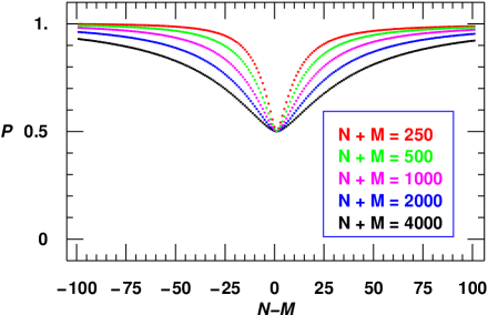
• As $|N-M|$ is increased, the value of $P_{1}$ in equilibrium, $\bar{P}_{1}$, increases and for large $|N-M|$ the system stops evolving, entering a “freeze-out” state. This trend can be clearly seen in Fig. 3. As further illustrated in Fig. 4, where $\bar{P}_{1}$ is plotted as a function of $N-M$ for fixed $M+N$, the minimum value of $\bar{P}_{1}=1/2$ occurs when $N=M$. That $\bar{P}_{1}$ rises for both signs of $(N-M)$ appears counterintuitive at first. Indeed, it means if we have a single spin up coupled to a very large system of spins down, the first spin does not equilibrate to a state mostly oriented down, but remains aligned up.

• As $|N-M|$ is increased, in addition to decay, the system start exhibiting oscillations, the frequency of which grows with $|N-M|$. The amplitude of these oscillations gets progressively smaller as $|M-N|$ increases, since the system approaches the freeze-out state. This behavior can be seen in Fig. 5, which reproduces at higher resolution the case $M=1280$, $N=2600$ of Fig. 3.

In what follows, we will discuss these features further. This will allow us to gain a deeper understanding of the spin system and its relationship to the neutrino system. We will first show how the transition from the regime in which the spins equilibrate to the freeze-out regime illustrates the interplay of “classical” and “quantum” effects. We will then discuss the time scale of the evolution and whether the system follows the predictions of the one-particle Hamiltonian in the classical regime. Finally, in Sect. V.3 we will comment on the periodicity of our solution.

Figure 4: The average probability ($\bar{P}_{1}=1/2+\sum_{J}C(J)$) when we change the number of spin ups and spin downs while keeping $M+N$ constant.

Figure 5: A close up of the plot for N=2560 and M=1280. Note the vertical scale. The probability is very close to one and fluctuates minimally about the average value.

V.1 From equilibration to freeze-out: a quantum-to-classical transition

In the course of the analysis in Sect. IV, we have encountered a situation in which fast coherent processes in the neutrino system corresponded to classical effects in the spin system, while slower incoherent processes in the neutrino system corresponded to quantum effects in the spin system. This physical picture is further illustrated by the system $m_{N}=N/2$, $m_{M}=-M/2$ we are now considering.

Once again, we recall that this system is reduced to two angular momenta as described in Sect. III.4. When $N$ and $M$ are large, these two angular momenta become approximately classical objects, $\vec{j}_{1}$ and $\vec{j}_{2}$. These objects are coupled with an interaction $const\times\vec{j}_{1}\cdot\vec{j}_{2}$. By energy conservation, this quantity stays fixed, and since the lengths of both vectors are fixed the angle between the vectors $\vec{j}_{1}$ and $\vec{j}_{2}$ stays fixed. Since the two vectors start out pointing in opposite directions, they remain pointing in opposite directions. The only possibility left is for the system to tilt as a whole, but that would violate momentum conservation, unless the total momentum of the system is zero ($N=M$). Thus, the classical system is frozen, unless $j_{1}=j_{2}$, which is a special point.

Our calculation shows that quantum mechanical effects actually resolve this discontinuity. The transition from the freeze-out to equilibration happens in some finite range of angular momenta.

What physics sets this range? Let us consider the two angular momenta being added as semiclassical objects. Then, in addition to the angular momenta in the $z$ direction, they each possess “quantum” angular momenta in the $x-y$ plane. These momenta are of the order

$$J_{xy}\sim\sqrt{J^{2}-J_{z}^{2}}=\sqrt{J(J+1)-J^{2}}=\sqrt{J}.$$

That this is a quantum effect is seen by restoring the units: $J_{xy}\sim\sqrt{J\hbar}$. This “quantum” angular momentum is what is responsible for the equilibration.

When the two angular momenta are added, their $x-y$ quantum momenta are also combined and the net object has $J_{x-y}$ of the same order as the ingredients. If the net classical momentum along the $z$ axis is greater then $J_{x-y}$, the equilibration will be suppressed. In other words, we arrive at the physical condition that determines the boundary between equilibration and “freeze-out”

$$|M-N|/2\sim\sqrt{(M+N)/2}.$$ (64)

For large number of spins, we can simply replace in this condition $\sqrt{(M+N)/2}\rightarrow\sqrt{N}$.

This boundary between freeze-out and equilibration can be quantified by the analytical expression for the equilibrium $P_{1}$ that can be derived for $|M-N|\ll(M+N)$ (see Appendix C):

$$\bar{P}_{1}\simeq 1-\frac{1}{1+\Delta/\Sigma}F\left(\frac{\Delta}{\sqrt{\Sigma}}\right),$$ (65)

Here, $\Delta\equiv(N-M)/2$, $\Sigma\equiv(M+N)/2$ and

$$F(a)\equiv\frac{1}{2}-\frac{a^{2}}{2}\int_{0}^{\infty}dy\frac{e^{-y}}{y+a^{2}}.$$ (66)

Up to a small correction in the prefactor in Eq. (65), $\bar{P}_{1}$ depends on $\Delta$ and $\Sigma$ in combination $\Delta^{2}/\Sigma$. Moreover, $F(a)$ quickly drops to zero as $a$ is increased beyond one. Hence, the width $|M-N|$ of the “quantum equilibration region” indeed scales with $N+M$ as $\sqrt{N+M}$.

This scaling can be seen in Fig. 4. The curves shown there are obtained by using the exact solution, Eqs. (16), (94), (95), (96). They are well described by Eq. (65).

V.2 Equilibration Time

We now discuss the time scales that control the evolution of our system. We are particularly interested to see how the evolution scales with the number of spins in the limit when the spin system is large.

As already mentioned, the case of $N=M$ considered in F&L II is straightforward: for large $N$ the evolution is uniquely dependent on $\sqrt{N}t$ and the decay curve is

$$P_{1}(t)=1-\frac{\sqrt{\pi}}{2}\sqrt{N}gt\exp(-Ng^{2}t^{2}){\rm erfi}(\sqrt{N}gt),$$ (67)

where ${\rm erfi}(z)$ is the imaginary error function

$${\rm erfi}(z)\equiv-i~{}{\rm erf}(iz)=\frac{2}{\sqrt{\pi}}\times\int_{0}^{z}\exp(t^{2})dt~{}.$$ (68)

Our investigations in Sect. V.1, however, showed that in general the situation is less obvious. For $N\neq M$ Figs. 3, 5 show a more complicated evolution pattern. Indeed, as we show next, in this case a new, shorter time scale enters the evolution.

First, let us consider the simplest example, an obvious limiting case $N=1$. As can be easily seen from Eq. (16), the evolution contains just a single oscillation frequency, as $J_{\rm min}=M/2-1/2$ and $J_{\rm max}=M/2+1/2$. The corresponding value of $\eta(M/2-1/2)$ is $2/(M+1)^{2}$. We thus have

$$P_{1}(t)=1-\frac{2}{(1+M)^{2}}+\frac{2}{(1+M)^{2}}\cos[gt(M+1)].$$ (69)

We see that the oscillation timescale grows linearly with the number of spins, not as a square root as in Eq. (67). We also notice that the amplitude of the oscillation is suppressed by the second power of the number of spins.

Next, let us consider a more nontrivial case $\sqrt{N+M}<|N-M|\ll(N+M)$. This case is characterized by the decay of the wavetrain to the value $\bar{P}_{1}$ given in Eq. (65). It turns out that for $\sqrt{N+M}<|N-M|\ll(N+M)$ the decay behavior is qualitatively different from Eq. (67). The wavetrain in this case is approximately described by

$$P_{1}(t) \simeq 1-\frac{\Sigma}{2}\left(\frac{1}{\Delta^{2}}-\frac{\cos\left(2gt\Delta+2\arctan\left(\frac{gt\Sigma}{\Delta}\right)\right)}{\Delta^{2}+g^{2}t^{2}\Sigma^{2}}\right).\;\;\;\;\;$$ (70)

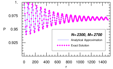
For details see Appendix D, where an asymptotic series for $P_{1}(t)$ is derived. Eq. (70) contains the leading term of this series. For sufficiently large $|M-N|$ (compared to $\sqrt{N+M}$) it gives an excellent approximation of the true result, as can be seen in Fig. 6.

Figure 6: Time evolution of $P_{1}(t)$ in the case $N=2300$, $M=2700$, $m_{N}=N/2$, $m_{M}=-M/2$. The Figure illustrates that Eq. (70) (curve) provides a very good approximation to the exact solution obtained by summing the series in Eqs. (16), (94), (95) (dots). The time variable is defined as $\tau\equiv gt(M+N)$, the same way as in Figs. 3, 5.

By inspecting Eq. (70), we clearly see that for nonzero $|M-N|$ a new frequency, $2g\Delta=g(N-M)$ enters the problem. We stress that this frequency depends on $N-M$ linearly. The amplitude of the oscillations at the maximum is suppressed by $(N+M)/|N-M|^{2}$, so as a function of $|M-N|$ the oscillations increase in frequency and decrease in amplitude. Finally, the oscillations decay with time as only a power law and the decay time, $t_{eq}\sim|N-M|/(g(N+M))$ increases with $|M-N|$. Compare this with the situation for $N=M$, in which case the decay time scale is $t_{eq}\sim 1/(g\sqrt{N})$ and the decay has exponential dependence.

At last, what conclusions can be drawn about the applicability of the one-particle coherent Hamiltonian in this case? Our conclusions is that one can define in what sense it is applicable, but the argument is a bit subtle. Unlike in the case $N=M$ considered in F&L II, in the more general setup considered here we find a new frequency, linearly dependent on the difference $|N-M|$. Can this be reconciled with Eq. (15), which states that in the neutrino system which begins as a collection of flavor eigenstates there should not be any flavor coherent conversion? We recall that while the frequency of our solution increases with $|N-M|$, the amplitude of the corresponding oscillations becomes smaller and smaller (see Eq. (70)). The oscillations become high-frequency as the system enters a state of freeze-out. The one-particle coherent limit corresponding to neglecting the residual small oscillations.

A different way to state this is that the oscillation amplitude is suppressed by $(M+N)/(N-M)^{2}$ and becomes large only when $|N-M|$ approaches $\sqrt{N+M}$. In the latter case, however, the oscillation frequency, obviously, becomes of order $\sqrt{N+M}$, and hence indistinguishable from the incoherent time scale.

V.3 The Period of the Probability

In this section we study the periodicity of the probability $P_{1}(t)$ observed in Fig. 3. Recall, the probability is

$$P(t)=const+\sum_{J=|j_{N}-j_{M}|}^{j_{N}+j2-1}\eta(J)\cos\left[gt\thickspace(2J+2)\right].$$ (71)

The periodicity is a consequence of the probability being a sum of cosines with frequencies that are multiples of the lowest, fundamental frequency.

V.3.1 The Case for N=1 or M=1

We first consider the case when N or M is one. Consider $N=1$. For this case there is only one cosine term with $J=\frac{M}{2}-\frac{1}{2}$. Therefore Eq. (71) reduces to,

$$P(t)=\sum_{J=|j_{N}-j_{M}|}^{j_{N}+j2}C(J)+\eta\left(\frac{M-1}{2}\right)\cos\left[gt\thickspace(M+1)\right]$$ (72)

Hence,

$$T_{N=1}=\frac{2\pi}{g(M+1)}$$ (73)

If we take $M=1$ instead, the result is the same except N and M are swapped.

V.3.2 The Case for $N>1$ and $M>1$

Each cosine in Eq.(71) satisfies,

$$\cos\left[gt\thickspace(2J+2)\right]=\cos\left[g(t+T_{J})(2J+2)\right]$$ (74)

Here $T_{J}$ is the period of the cosine corresponding to angular momenta $J$. Now for all $J$,

$$T_{J}=\frac{2\pi}{g(2J+2)}$$ (75)

To find the period we need the least common multiple of the $T_{J}$’s. We find the period (together with the previous subsection) to be,

$$T=\begin{cases}\frac{\pi}{g},&\text{ if $N+M=$ even (or J=integer)}\\ \frac{2\pi}{g},&\text{ if $N+M=$ odd (or J= half integer)}\\ \frac{2\pi}{g(N+M)},&\text{ if N=1 or M=1}\end{cases}$$ (76)

Note that the period is the same for the case of a flavor eigenstate background and a flavor superposition background because the period only depends on the argument of the cosine. The argument of the cosine is the same for both cases. The discontinuity between the period when $N=1$ or $M=1$ and the other cases arises because in the first two cases there is an interference of many cosine waves (as there the cosines are summed over) and in the last case there is only one cosine wave. For $M=N$, our results reduce to that found in F&L II.

Notice that, up to the factor of two controlled by whether $N+M$ is even or odd, the period of the spin system depends only on the value of the spin-spin coupling $g$ and not on the size of the spin system. For a neutrino system, $g=\frac{\sqrt{2}G_{F}}{V}$ and the period seems to depend on the volume occupied by the neutrino system. In fact, in a real neutrino gas, non-forward scattering effects would destroy any periodicity. We recall that for sufficiently large numbers of neutrinos the time scale of incoherent forward scattering, Eq. (14), is much smaller than the period found here and, moreover, that forward incoherent scattering is only a small fraction of the total incoherent scattering (see F&L II). Thus, the periodicity is an example of an effect in the spin system that is not realized in the actual neutrino system. In the context of the spin system, on the other hand, the effect is perfectly physical and indeed is reminiscent of the well-known “spin echo” effect experimentally observed in actual spin systems.

Figure 7: Plots of $N=2560$ and various numbers of spin down particles, $M$. The time is scaled so that $\tau=gt(M+N)$. Note that for all the graphs $N+M=$odd

As a final comment note that when we approximate the sums over the cosines by the integrals, in Eqs. (59), (65), and (70), the periodicity of the solution is destroyed. This has to do with the disappearance of the fundamental (lowest) frequency in the system. The same observation was made in F&L II for $N=M$.

V.3.3 A note about minima

Let us call the case when $P_{1}=1/2+\sum_{J}C(J)-\sum_{J}\eta(J)$ (which is the lowest possible value that the probability can be) a perfect minimum. For the perfect minimum to occur we must have, $\cos\left[gt\thickspace(2J+2)\right]=-1$ simultaneously for all $J$. The period of each cosine decreases as $J$ increases, therefore we only need to find the time when the cosine with the largest period and the cosine with the smallest period are simultaneously equal to $-1$.

By a calculation analogous to that for the period one can show that if $N+M=$ even there will never be a perfect minimum. If $N+M$ is odd the times when the probability attains a perfect minimum is,

$$T_{min}=\frac{k\pi}{g}\hskip 14.22636pt{\rm where}\hskip 14.22636ptk=1,2,3...$$ (77)

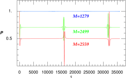
Note that this is half way between perfect maxima (the case where $P_{1}(t)=1/2+\sum_{J}C(J)+\sum_{J}\eta(J)$). Hence if $M+N$ is odd (or $J$ is half an integer) the probability has both a perfect minimum and a perfect maximum. This result shows yet another intriguing physical feature of the spin system. While a system with $N+M=$ even is characterized by a set of recurring maxima, in the system with $N+M=$ odd every other such maximum is replaced by a minimum. This behavior is illustrated in Fig. 7. Note that in this figure, as before, the abscissa is the scaled time $\tau=gt(M+N)$.

VI The freeze-out effect and a real neutrino gas: a critical analysis

VI.1 Overview of the problem

In Sect. V we found that a general “$N+M$” ($N\neq M$) spin system that starts polarized in the $z$ direction typically equilibrate very little, even on the longer incoherent time scale, except in cases when $N$ and $M$ are very close ($|N-M|\lesssim\sqrt{N}$). Obviously, it is important to understand if this finding corresponds to the behavior of a real neutrino gas. This question is not a trivial one. As mentioned in the introduction, going from a neutrino gas to the spin model involves several simplifying assumptions: only forward scattering is kept, equal interaction strengths are assumed, the interactions are taken to be continuous in time, etc. All these assumptions could, in principle, introduce certain artifacts in the system and it is not a priori obvious that the freeze-out behavior found in the toy model is not just such an artifact. We will examine this question next.

VI.2 Interference of neutrino scattering amplitudes

Consider a test neutrino, taken for definiteness to be $|\nu_{e}>$, flying though a box with the gas of neutrinos. Assume the neutrinos in the gas are in the flavor eigenstates,

$$|S(0)\rangle=|\underbrace{\nu_{e}\nu_{e}...\nu_{e}}_{(N-1)}\underbrace{\nu_{\mu}\nu_{\mu}...\nu_{\mu}}_{M}\rangle~{}.$$ (78)

Let us limit scattering to only the forward process and ask: what is the probability that scattering changes flavor of the test neutrino?

Let us review the arguments of F&L I. Omitting the flavor-preserving neutral current piece, which is the same for all neutrinos, we can write the result of the interaction to first order in the interaction amplitude $a$ as

$$|\nu_{e}\rangle|\underbrace{\nu_{e}\nu_{e}...\nu_{e}}_{(N-1)}\underbrace{\nu_{\mu}\nu_{\mu}...\nu_{\mu}}_{M}\rangle\longrightarrow$$

$$|F\rangle = (1+(N-1)ia)|\nu_{e}\rangle|\nu_{e}\nu_{e}...\nu_{e}\nu_{\mu}\nu_{\mu}...\nu_{\mu}\rangle$$ (79)

$$+ ia(\underbrace{|\nu_{\mu}\rangle|\nu_{e}\nu_{e}...\nu_{e}\nu_{e}\nu_{\mu}...\nu_{\mu}\rangle+|\nu_{\mu}\rangle|\nu_{e}\nu_{e}...\nu_{e}\nu_{\mu}\nu_{e}...\nu_{\mu}\rangle+...}_{M}),$$

The interaction amplitude $a$ is given by $a\equiv C\delta t\equiv-\sqrt{2}G_{F}(1-\cos\Theta)\delta t/V$ Friedland_&_Lunardini_1 ; Friedland_&_Lunardini_2 , where $\delta t$ is the duration of the interaction between a pair of neutrinos. Since the final states are mutually orthogonal, the probability of flavor change goes as $Ma^{2}$ indicating the incoherent nature of the evolution.

Eq. (VI.2) assumes that the time step $\delta t$ is small such that not only $C\delta t\ll 1$, but also $NC\delta t\ll 1$ are satisfied. While the former is indeed true for any reasonable neutrino system of interest Friedland_&_Lunardini_2 , the latter need not hold, as $Na$ or $Ma$ for large $N$ and $M$ are not necessarily small. To make contact with the spin system, which stays continuously coupled, we must consider longer interaction times. Correspondingly, we need to modify Eq. (VI.2), keeping higher powers of $a$.

One can accomplish this by regarding (VI.2) as the first order term in the perturbative expansion of the wavefunction at the time $\delta t$ ($NC\delta t\ll 1$, $MC\delta t\ll 1$), and using this to make further steps in time to the time $T=n\delta t$ ($CT\ll 1$, but not necessarily $NCT\ll 1$, $MCT\ll 1$). Let us define a convenient notation of the initial state

$$|I\rangle=|\nu_{e}\rangle|\underbrace{\nu_{e}\nu_{e}...\nu_{e}}_{(N-1)}\underbrace{\nu_{\mu}\nu_{\mu}...\nu_{\mu}}_{M}\rangle$$ (80)

and the “exchange” state

$$|E\rangle = \underbrace{|E_{1}\rangle+|E_{2}\rangle+...}_{M},$$ (81)

$$|E_{1}\rangle = |\nu_{\mu}\rangle|\nu_{e}\nu_{e}...\nu_{e}\nu_{e}\nu_{\mu}...\nu_{\mu}\rangle,$$ (82)

$$|E_{2}\rangle = |\nu_{\mu}\rangle|\nu_{e}\nu_{e}...\nu_{e}\nu_{\mu}\nu_{e}...\nu_{\mu}\rangle,$$ (83)

$$...$$

Then at the time $T$ the state is

$$|T=n\delta t\rangle = \left(1+i(N-1)C\delta t\right)^{n}|I\rangle$$ (84)

$$+ iC\delta t\left[\sum_{r=0}^{n-1}\left(1+i(N-1)C\delta t\right)^{n-1-r}\left(1+i(M-1)C\delta t\right)^{r}\right]|E\rangle$$

$$+ O([iC\delta t]^{2}),$$

as can be readily verified by induction.

The cyclotomic polynomial is summed to give

$$|T=n\delta t\rangle = \left(1+i(N-1)C\delta t\right)^{n}|I\rangle$$ (85)

$$+ iC\delta t\frac{\left(1+i(N-1)C\delta t\right)^{n}-\left(1+i(M-1)C\delta t\right)^{n}}{iC(N-M)\delta t}|E\rangle$$

$$+ O([iC\delta t]^{2}),$$

and, taking the limit $n\to\infty$

$$|T=n\delta t\rangle = e^{i(N-1)CT}|I\rangle$$ (86)

$$+ \frac{\left(e^{i(N-1)CT}-e^{i(M-1)CT}\right)}{(N-M)}|E\rangle$$

$$+ O([iC\delta t]^{2}).$$

Note that the explicit dependence on $\delta t$ has now disappeared. This is to be expected since the formal solution of the Schrödinger equation for the system depends only on the time difference between the initial and final times.

The reason for the freeze-out behavior is now clear. For large values on $N-M$, the probability of a transition to the exchange state is suppressed by the factor $(N-M)^{-2}$.

Notice first of all that this effect disappears when $N=M$. This is why in this case one can observe full equilibration and test the incoherent nature of the evolution. However, one should note that in the present approximation the $N\to M$ limit gives $iCT$ as the amplitude for the state $|E\rangle$. As in this case the phase of the initial and exchange states are the same, we regard one factor of $T$ in the probability as a relic of the energy conservation delta function, and obtain as the probability per unit time for a transition from the initial state

$$\frac{dP}{dt}=M|C|^{2}$$ (87)

(remember that $\langle E|E\rangle=M$), showing incoherent equilibration.

VI.3 Does the freeze-out happen in a real neutrino system?

Finally, we can address the key question: does the freeze-out observed in the model of interacting spins actually happen in a real neutrino system? The answer is negative.

Let us return to the arguments in the previous subsection. Upon closer inspection of Eq. (VI.2), it becomes clear that for large $N$, $M$ and times $T\ll C^{-1}$, the problem is in fact equivalent to an oscillation set-up with a Hamiltonian that, in the basis $|I\rangle,|E_{1}\rangle,|E_{2}\rangle,...$, has $(iCN,iCM,iCM,iCM,...)$ on the diagonal and factors of $iC$ on the off-diagonal, in the first column (and the corresponding terms in the first row). For the case $N=M$ considered in Friedland_&_Lunardini_2 , the transition probability between $|I\rangle$ and any of the states $|E_{i}\rangle$ is given by $P\sim|itC|^{2}$. The generalization of this to $N\neq M$ is

$$P\sim\left\arrowvert i\times C\times\int_{0}^{T}dt\exp[i(N-M)t\times C]\right\arrowvert^{2}.$$ (88)

It is straightforward to check that the transition probability that follows from Eq. (88)

$$P \sim \left\arrowvert\frac{\exp[iC(N-M)T]-1}{(N-M)}\right\arrowvert^{2}$$ (89)

$$= \frac{2-2\cos((N-M)CT)}{(N-M)^{2}}$$

agrees with that obtained from Eq. (86), indicating that the corresponding amplitudes are the same, up to an overall phase convention.

Let us take the time $T$ in Eq. (88) to be the timescale of incoherent equilibration, given by Eq. (14):

$$t_{\rm eq}^{inc}\sim(G_{F}\sqrt{(N+M)/2}/V)^{-1}.$$ (90)

If $N=M$, the probability to transition into any one of the exchange states $|E_{i}\rangle$ in this time is $P\sim(Ct_{\rm eq}^{inc})^{2}$. Remembering that $C=-\sqrt{2}G_{F}/V(1-\cos\Theta)$ and dropping the angular factor $(1-\cos\Theta)$ (which is also dropped in the derivation of Eq. (90)), we get $P\sim((N+M)/2)^{-1}$. The probability of transition into any of the exchange states is $P(|I\rangle\rightarrow|E_{any}\rangle)\sim(N-1+M)P\sim 1/2$, thus confirming that the equilibration does happen on the time scale $t_{\rm eq}^{inc}$.

If, however, we have $(N-M)CT\gtrsim 1$, the oscillating exponent in Eq. (88) suppresses the transition and the system freezes out. Thus, we immediately obtain a physical estimate for the freeze-out:

$$|N-M|\sqrt{2/(N+M)}\gtrsim 1,$$ (91)

which is nothing but the condition we found in the spin system, Eq. (64), up to a trivial factor. This provides a powerful check of the validity of Eq. (88) and the physical picture that led to it.

We can now give interpret Eq. (88) the following interpretation. For $N$, $M\gg 1$, the states $|I\rangle$, $|E_{i}\rangle$ are approximately energy eigenstates. Strictly speaking, of course, the true energy eigenstates are mixtures of $|I\rangle$, $|E_{i}\rangle$, but for large $N$, $M$ one of the eigenstates is predominately $|I\rangle$, with a small admixture of the other states, and vice versa. Correspondingly, we can loosely speak of the energies of the $|I\rangle$ and $|E_{i}\rangle$ states. For $N\neq M$ the state $|I\rangle$ and any of the states $|E_{i}\rangle$ have different energies. The incoherent spin flips in the spin system are thus forbidden by energy conservation (enforced by the oscillating exponent in Eq. (88)).

In a real neutrino system, of course, there is an additional degree of freedom: the neutrino momentum. The energy liberated in the process of flavor exchange is converted into a slight shift of the neutrino kinetic energy and the energy conservation is assured. In the simplest manifestation of this point, a neutrino existing a dense neutrino region will gain a small amount of kinetic energy. (The neutrino-neutrino interactions, just like any interactions between like particles mediated by a vector boson, are repulsive.)

Thus, the freeze-out observed in the spin model is an artifact of the model, more specifically, a consequence of the dropped degrees of freedom, neutrino momenta.

This discussion applies to the system of neutrino plane waves in a box, which was the system for which the spin model was created. It is instructive to instead consider a system of interacting neutrino wavepackets. In this system the interaction energy is localized to the regions occupied by the overlapping wavepackets, with the total interaction energy (averaged over volume) being the same as in the case of plane waves. The statement of the changing kinetic energy, as the neutrino moves from a more dense to a less dense region, has its analogue in the case of wavepackets as well: The kinetic energy of a given packet changes as it interacts with another packet. Upon spatial averaging this change, one gets the “plane waves” result. There are fewer interactions in less dense regions, hence the averaged kinetic energy there is higher.

The advantage of thinking about wave packets is that in this case it is clear that the rate of incoherent scattering cannot be suppressed: for sufficiently small wavepackets they interact with each other two-at-a-time, giving the usual scattering rate. The answer in the physical system cannot depend on the size of the wavepackets, since the interaction Hamiltonian is energy-independent.

VII Conclusions

No problem in physics can be solved exactly. Often, however, a given physical problem could be mapped onto an idealized system, for which a complete solution exists. One then needs to critically examine which features of the solution carry through to the original physical system and which arise as artifacts of the simplifying assumptions made along the way.

We have performed just such an analysis. Our goal was to investigate coherent effects in a gas of neutrinos. We have simplified the system by limiting the scattering to only forward direction and omitting the momentum degrees of freedom. With only the flavor degrees of freedom remaining, the neutrino system could be mapped onto a system of coupled spins. We further simplified the problem by setting the coupling strengths to be equal, and considering a certain class of initial states. We have shown that the resulting spin model could be solved exactly. Our solution generalizes the analysis of F&L II Friedland_&_Lunardini_1 , where a particular initial state, the one with equal numbers of up and down spins, was considered.

The solution proved to be very instructive. The spin system exhibited both coherent oscillations and incoherent decay, reproducing effects expected for a real neutrino gas. Several examples were considered in Sects. IV and V. As these examples demonstrate, coherent effects in the neutrino system correspond to the behavior of the spin system in the classical limit; likewise, incoherent effects in the former have their analogue in quantum effects in the latter.

We have presented two different methods of obtaining the solution. The first construction separates the system in three parts: the test spin, the other spins that started in the same orientation and the remaining spins. The second method exploits the high degree of symmetry of our chosen initial states. Both methods have complementary advantages. The second of the methods provided crucial physical intuition for understanding the classical limit of the system and the interplay of quantum and classical effects, as shown in Sects. IV and V.1. At the same time, the first method is more general and can be used to generate solutions for any initial state of the test spin (by simply changing the state of the test spin by adjusting the parameter $\lambda$ in Sect. III.3.3 ).

Several interesting results were found. One such result involves the subtlety of identifying coherent effects in the neutrino system by taking a classical limit of the spin system. The special case considered in Friedland_&_Lunardini_1 seemed to suggest that in the large $N$ quantum effects separate from classical ones necessarily by having longer time scales (scaling as a square root in the number of particles). What we found in Sect. V.2 is that some quantum effects instead decouple by having a vanishing amplitude, while their frequency scales as if they were classical effects.

Another interesting finding of our analysis is that in certain spin systems the evolution does not lead to equilibration, even on the incoherent time scales. For example, the system considered in Sect. V is “frozen-out”, unless the initial numbers of spins up and down are very close. By studying this example and comparing it to the case considered in Sect. IV we conclude the freeze-out happens in the spin system for any mode where quantum effects are suppressed a large classical (coherent) effect. We have seen, e.g., in Sect. V.1 that equilibration is precluded by the conservation of the classical angular momentum. Only when the classical angular momentum is reduced to the level comparable to the quantum effects is the equilibration allowed to proceed. The special case considered in Friedland_&_Lunardini_1 falls into the latter category.

We have explained in Sect. VI that the physical origin of the freeze-out effect comes from dropping the momentum degrees of freedom of the neutrino system. While the freeze-out certainly happens in the spin system, it does not happen in a real neutrino gas. This gives an important example of the limitations of the spin model: while it captures all coherent effects in the neutrino system, it does not always capture incoherent effects, only those that are not classically suppressed.

In addition to giving the full solution in Eqs. (16), (19), and (22), in several case we have derived approximate expressions that elucidate the physics of the system. For example, Eq. (59) cleanly demonstrates the presence of both oscillation and decay in the spin system. Eq. (65) helps to understand the interplay of classical and quantum effects in the processes of equilibration and freeze-out. Finally, Eq. (70) showed the subtlety of decoupling the quantum effect in the classical limit.

We believe that our extensive investigation here will contribute to better understanding of the flavor evolution in dense neutrino systems. We also hope that our results could find applications beyond the neutrino field.

Appendix A Explicit expressions for $C(J)$ and $\eta(J)$

Eqs. (16), (19), (22) give the general form of the solution for the probability $P_{1}(t)$. Here we give explicit expressions for $C(J)$ and $\eta(J)$ for the specific cases analyzed in the text.

In Sec. IV we consider the initial state containing $N$ spin up particles ($m_{N}=N/2$) and $M$ spins in the orthogonal direction ($m_{M}=0$). In this case, Eqs. (19) (22), upon evaluating the Clebsch-Gordan, $3j$- and $6j$-coefficients, become

$$C(J) = \frac{(1+2J)[\Delta(1+\Sigma)+J(1+J)]}{4J(1+J)\Gamma[1+J-N/2]\Gamma[1+J+\Delta]}$$ (92)

$$\times \frac{\Gamma[1+J+\Delta]\Gamma[1+J+N/2]\Gamma[N+1]}{\Gamma[\Sigma-J+1]\Gamma[\Sigma+J+2]},$$

$$\eta(J) = \frac{\Gamma[2+J+\Delta]\Gamma[2+J+N/2]\Gamma[N]}{(1+J)\Gamma[1+J-N/2]\Gamma[1+J+\Delta]}$$ (93)

$$\times \frac{1}{\Gamma[\Sigma-J]\Gamma[\Sigma+J+2]}.$$

Here $\Delta\equiv\frac{N-M}{2}$ and $\Sigma\equiv\frac{N+M}{2}$.

Similarly, in Sec. V we consider the initial state containing $N$ spin up particles ($m_{N}=N/2$) and $M$ spin down particles ($m_{M}=-M/2$). In this case, Eqs. (19), (22) evaluate to

$$C(J) = \frac{(1+2J)M\Delta[\Delta(1+\Sigma)+J(1+J)]}{2J(1+J)}$$ (94)

$$\times \frac{\Gamma(M)\Gamma(N)}{\Gamma[\Sigma-J+1]\Gamma[\Sigma+J+2]},$$

$$\eta(J) = \frac{M[(1+J)^{2}-\Delta^{2})\Gamma(M)\Gamma(N)}{(1+J)\Gamma[\Sigma-J]\Gamma[\Sigma+J+2]}.$$ (95)

Eq. (94) is ambiguous for $J=0$. In this case, which occurs only when $N=M$, we have

$$C(0) = 0.$$ (96)

Formally, this can be seen from Eq. (19), in which both the $3j$- and the $6j$-symbols contain objects that do not form closed triangles and hence vanish.

Notice that our expressions agree with the solution given in F&L II Friedland_&_Lunardini_1 in the case $N=M$. Indeed, setting $M=N$, $x=0$, and $y=N$ we have $C(J)=0$ and $\eta(J)=(1+J)N[(N-1)!]^{2}/[(N-J-1)!(N+J+1)!]$. Noticed that Eq. (4.6) in the journal version of Friedland_&_Lunardini_1 contains a typo: the factor $(1+2J)$ in the numerator should be $(2+2J)$ (the first line of that equation is correct).

Appendix B Derivation of Eq. (59)

The derivation of Eq. (59) proceeds as follows. Let us start with the definition of $\eta(J)$ in Eq. (22). Approximating the gamma functions by the Sterling formula, $\Gamma(z)=(z-1)!\simeq\sqrt{2\pi}e^{(z-1/2)\ln(z-1)-(z-1)}$, and combining the resulting exponents, we get

$$\eta(J) = \frac{1}{(1+J)\sqrt{2\pi}}\exp[A],$$

$$A \equiv \frac{1}{2}\left((3+2J+M-N)\ln\left[\frac{2+2J+M-N}{2}\right]\right.$$ (97)

$$+ \left.(3+2J+N)\ln\left[\frac{2+2J+N}{2}\right]\right.$$

$$- \left.(2J-N+1)\ln\left[\frac{2J-N}{2}\right]\right.$$

$$- \left.(2J-M+N+1)\ln\left[\frac{2J-M+N}{2}\right]\right.$$

$$+ \left.(2N-1)\ln[N-1]\right.$$

$$+ \left.(1+2J-M-N)\ln\left[\frac{-2-2J+M+N}{2}\right]\right.$$

$$- \left.(3+2J+M+N)\ln\left[\frac{2+2J+M+N}{2}\right]\right.$$

$$- \left.2\right).$$

We need to find the maximum of $A$ and expand $A$ in a series in $J$ to the second order around this maximum. A derivative $\partial A/\partial J$ has two types of terms: logarithms and terms that go like $1/\#$, where “#” denotes an expression linear in $J$, $N$, and $M$. Clearly, for sufficiently large values of $N$ and $M$ the logarithms dominate. The maximum is then found by combining the logarithms and setting the argument of the combined logarithm to 1. This yields

$$\frac{(2+2J+M-N)(2+2J+N)}{(2J-N)(2J-M+N)}$$ (98)

$$\times \frac{-2-2J+M+N}{(2+2J+M+N)}=1.$$

For large $N$ and $M$, we can drop small numbers compared to $J$, $M$, $N$. The above equation then gives the answer

$$J_{\rm max}=\frac{\sqrt{M^{2}+N^{2}}}{2},$$ (99)

which is exactly the answer for the classical problem.

Upon evaluating the second derivative, $\partial^{2}A/\partial J^{2}$, we again find two types of terms, some that go like $1/\#$ and some that go like $1/\#^{2}$. Keeping only the terms of the first kind, substituting Eq. (99), and simplifying, we get

$$\partial^{2}A/\partial J^{2}=-\left(\frac{4}{N}+\frac{4N}{M^{2}}\right)$$ (100)

Finally, we need to find the value of $A$ in Eq. (B) for $J=J_{\rm max}$. This involves a rather lengthy calculation involving a lot of cancellations. All terms of the type $J\ln[\#]$, $N\ln[\#]$, and $M\ln[\#]$ cancel out, when Eq. (98) is used. The terms of the type $\ln[\#]$ give $\ln(M^{2}/(4N))$ upon simplification. Finally, the order one terms also cancel out. Thus, we get

$$A_{J_{\rm max}}=\ln\left(\frac{M^{2}}{4N}\right)+O\left(\frac{1}{N},\frac{1}{M},\frac{1}{J}\right),$$ (101)

or

$$A\simeq\frac{1}{2}\ln\left(\frac{M^{2}}{4N}\right)-\left(\frac{2}{N}+\frac{2N}{M^{2}}\right)(J-\sqrt{M^{2}+N^{2}}/2)^{2}$$ (102)

This means that $\eta(J)$ is a Gaussian centered at $J_{\rm max}=\frac{\sqrt{M^{2}+N^{2}}}{2}$. For large $N$, $M$ the Gaussian is sufficiently narrow and we can replace the prefactor $1/(1+J)$ by $2/\sqrt{M^{2}+N^{2}}$. The sum over $J$ in Eq. (16) can be replaced by an integral, in which we can extend the limits of integration to $\pm\infty$. We have

$$\int_{-\infty}^{\infty}dJ\eta(J)\cos(2gJt)=$$ (103)

$$\frac{2}{\sqrt{2\pi}\sqrt{M^{2}+N^{2}}}\left(\frac{M^{2}}{4N}\right)^{1/2}\int_{-\infty}^{\infty}dJe^{-\left(\frac{2}{N}+\frac{2N}{M^{2}}\right)\left(J-\frac{\sqrt{M^{2}+N^{2}}}{2}\right)^{2}}\cos(2gJt)=$$

$$\frac{\sqrt{2}}{\sqrt{\pi}\sqrt{M^{2}+N^{2}}}\left(\frac{M^{2}}{4N}\right)^{1/2}\frac{\sqrt{\pi}\sqrt{NM^{2}}}{\sqrt{2(M^{2}+N^{2})}}e^{-\left(\frac{2}{N}+\frac{2N}{M^{2}}\right)^{-1}g^{2}t^{2}}\cos(g\sqrt{M^{2}+N^{2}}t)=$$

$$\frac{1}{2}\frac{M^{2}}{(M^{2}+N^{2})}e^{-\left(\frac{2}{N}+\frac{2N}{M^{2}}\right)^{-1}g^{2}t^{2}}\cos(g\sqrt{M^{2}+N^{2}}t).$$

The constant term $1/2+\sum_{J=J_{\rm min}}^{J_{\rm max}}C(J)$ can be immediately found as the difference between $1$ and the oscillating term at $t=0$:

$$1-\frac{1}{2}\frac{M^{2}}{(M^{2}+N^{2})}=\frac{1}{2}+\frac{1}{2}\frac{N^{2}}{(M^{2}+N^{2})}.$$ (104)

This concludes the derivation of Eq. (59).

Appendix C Derivation of Eq. (65)

To find the constant value $\bar{P}_{1}$ to which $P_{1}(t)$ relaxes we can either compute the sum $1/2+\sum_{J=J_{\rm min}}^{J_{\rm max}}\tilde{C}(J)$, or use the trick at the end of Appendix B and compute $1-\sum_{J=J_{\rm min}}^{J_{\rm max}-1}\eta(J)$. Let us do the latter.

The first step is to approximate the gamma functions in Eq. (95) by the Sterling formula and expand the exponent. After a fairly straightforward calculation, one finds a Gaussian in $J+1$:

$$\frac{\Gamma(M+1)\Gamma(N)}{\Gamma[(M+N)/2-J]\Gamma[(M+N)/2+J+2]}\simeq$$

$$\exp\left[B-\frac{2(M+N-1)}{(M+N)^{2}}(J+1)^{2}\right],$$ (105)

where

$$B \equiv \left(M+\frac{1}{2}\right)\log M+\left(N-\frac{1}{2}\right)\ln(N-1)$$ (106)

$$- (1+M+N)\ln\left(\frac{M+N}{2}\right)+1$$

For definitiveness, let us take $M>N$ and let us assume that $(M-N)\ll N$. We can then expand Eq. (106) in series in $\Delta$:

$$B \simeq \left(N-\frac{1}{2}\right)\ln(N-1)-\left(N+\frac{1}{2}\right)\log N$$ (107)

$$+ 1+\frac{2N-1}{8N^{2}}(N-M)^{2}$$

$$= -\ln N+\frac{1}{4N}(N-M)^{2}+O(1/N^{2}).$$

We have

$$\eta(J) \simeq \frac{[(1+J)^{2}-\Delta^{2}]}{(1+J)(\Delta+\Sigma)}\exp\left[\frac{\Delta^{2}}{\Delta+\Sigma}-\frac{(J+1)^{2}}{\Sigma}\right],\;\;\;\;$$ (108)

where, as before, $\Delta\equiv\frac{N-M}{2}$ and $\Sigma\equiv\frac{N+M}{2}$.

Let us approximate the sum over $J$ by an integral

$$\bar{P}_{1}=1-\sum_{J=(M-N)/2}^{(M+N)/2-1}\eta(J)$$ (109)

$$\rightarrow 1-\int_{\Delta}^{\Sigma-1}dJ\frac{(J^{2}-\Delta^{2})}{J(\Delta+\Sigma)}\exp\left[\frac{\Delta^{2}}{\Delta+\Sigma}-\frac{J^{2}}{\Sigma}\right].$$

Let us shift the integration variable $\tilde{J}=J-\Delta$ and extend the upper limit of integration to infinity:

$$1-\bar{P}_{1}\simeq$$ (110)

$$\int_{0}^{\infty}d\tilde{J}\frac{(\tilde{J}+2\Delta)\tilde{J}}{(\tilde{J}+\Delta)(\Delta+\Sigma)}\exp\left[\frac{\Delta^{2}}{(\Delta+\Sigma)}-\frac{(\tilde{J}+\Delta)^{2}}{\Sigma}\right].$$

Introducing a new variable $\xi=\tilde{J}/\sqrt{\Sigma}$, we get

$$1-\bar{P}_{1}\simeq\frac{\Sigma}{\Delta+\Sigma}\exp\left[\frac{-\Delta^{3}}{(\Delta+\Sigma)\Sigma}\right]F\left(\frac{\Delta}{\sqrt{\Sigma}}\right),$$ (111)

where

$$F(a)\equiv\int_{0}^{\infty}d\xi\frac{(\xi+2a)\xi}{(\xi+a)}\exp\left[-(\xi^{2}+2\xi a)\right]$$ (112)

The function $F(a)$ drops to zero quickly as $a$ is increased beyond one. Since the argument of $F$ in Eq. (111) is $\Delta/\sqrt{\Sigma}$, we conclude that indeed $\bar{P}_{1}\rightarrow 1$ for $\Delta\gtrsim\sqrt{\Sigma}$.

For $\Delta\lesssim\sqrt{\Sigma}$ the argument of the exponent in Eq. (111) is of the order $\Delta^{3}/\Sigma^{2}\lesssim\Sigma^{-1/2}$ and hence in the limit of a large number of spins the exponent can be set to one.

The integral defining the function $F(a)$ can be further transformed as follows:

$$F(a) = \int_{0}^{\infty}d\xi\frac{(\xi+a)^{2}-a^{2}}{\xi+a}\exp\left[-(\xi+a)^{2}\right]e^{a^{2}}$$ (113)

$$= e^{a^{2}}\int_{0}^{\infty}d\xi\left((\xi+a)-\frac{a^{2}}{\xi+a}\right)\exp\left[-(\xi+a)^{2}\right]$$

$$= \frac{1}{2}-\frac{e^{a^{2}}}{2}\int_{0}^{\infty}d(\xi+a)^{2}\frac{a^{2}}{(\xi+a)^{2}}\exp\left[-(\xi+a)^{2}\right]$$

$$= \frac{1}{2}-\frac{a^{2}}{2}\exp[a^{2}]\int_{a^{2}}^{\infty}dy\frac{e^{-y}}{y}$$

Finally, we arrive at

$$\bar{P}_{1}\simeq 1-\frac{\Sigma}{\Delta+\Sigma}F\left(\frac{\Delta}{\sqrt{\Sigma}}\right),$$ (114)

where

$$F(a)=\frac{1}{2}-\frac{a^{2}}{2}\int_{0}^{\infty}dy\frac{e^{-y}}{y+a^{2}}.$$ (115)

The function $F(a)$ equals $1/2$ at $a=0$ ($F(a)\stackrel{{\scriptstyle a\rightarrow 0}}{{=}}1/2+1/2(2\ln a+\gamma)a^{2}+1/2(2\ln a+\gamma-1)a^{4}+...$, $\gamma\simeq 0.577216$ being the Euler constant). As $a\rightarrow\infty$ $F(a)$ approaches $0$ ($F(a)\stackrel{{\scriptstyle a\rightarrow\infty}}{{=}}a^{-2}/2+...$).

Appendix D Derivation of Eq. (70)

In Sect. V we consider the evolution of the spin system in which all spins are initially in flavor eigenstates. In this Appendix we derive an approximate expression describing this evolution in the regime when $\sqrt{M+N}<|M-N|\ll(M+N)$.

The time dependent part of the evolution is given by $\sum_{J}\eta(J)\cos(2gt(J+1))$. The coefficient $\eta(J)$ depends on $\Delta=(N-M)/2$ and can be usefully approximated for the case when $\Delta$ is small by Eq. (108) of Appendix C.

As before, we approximate the sum by an integral

$$\sum_{J=(M-N)/2}^{(M+N)/2-1}\eta(J)\cos(2gt(J+1))$$

$$\rightarrow \int_{\Delta}^{\Sigma-1}dJ\frac{(J^{2}-\Delta^{2})}{J(\Delta+\Sigma)}\exp\left[\frac{\Delta^{2}}{\Delta+\Sigma}-\frac{J^{2}}{\Sigma}\right]\cos(2gtJ),$$

shift the variable, $J$ to $\tilde{J}=J-\Delta$, and extend the range of integration to infinity. We find

$$\sum_{J=(M-N)/2}^{(M+N)/2-1}\eta(J)\cos(2gt(J+1)) \simeq \exp\left[\frac{-\Delta^{3}}{(\Delta+\Sigma)\Sigma}\right]\frac{1}{(\Delta+\Sigma)}$$ (117)

$$\times \int_{0}^{\infty}dJ\frac{(\tilde{J}+2\Delta)\tilde{J}}{(\tilde{J}+\Delta)}\exp\left[-\frac{\tilde{J}^{2}}{\Sigma}-\frac{2\tilde{J}\Delta}{\Sigma}\right]\cos(2gt(\tilde{J}+\Delta)).$$

F&L II considered a limit $\Delta=0$. In that case the integral equals

$$\frac{1}{2}-\frac{\sqrt{\pi}}{2}\sqrt{N}gt\exp(-Ng^{2}t^{2}){\rm erfi}(\sqrt{N}gt),$$ (118)

from which Eq. (67) immediately follows.

We notice that the values of $\tilde{J}$ that contribute in the case $\Delta=0$ are of the order $\sqrt{\Sigma}$, as the integral in Eq. (117) is cut off by the term $\exp(-\tilde{J}^{2}/\Sigma)$. If we take $\Delta>\sqrt{\Sigma}$, however, we find that the integral is first cut off by the exponential term $\exp(-2\tilde{J}\Delta/\Sigma)$, at $\tilde{J}\sim\Sigma/2\Delta$. If $\Delta$ is sufficiently large, we may evaluate the integral in Eq. (117) with the first term in the exponent dropped. The integral then becomes

$$\int_{0}^{\infty}d\tilde{J}\frac{(\tilde{J}+2\Delta)\tilde{J}}{(\tilde{J}+\Delta)}\exp\left[-\frac{2\tilde{J}\Delta}{\Sigma}\right]\cos(2gt(\tilde{J}+\Delta)).$$ (119)

We next take advantage of the fact that integrals of the form $\int_{0}^{\infty}dx\;x^{n}\exp[-x]\cos(x+\alpha)$ can be done and the answer has a simple and useful analytic form

$$\int_{0}^{\infty}dxx^{n}\exp\left[-Ax\right]\cos[B(x+\alpha)]=$$

$$\frac{n!}{(A^{2}+B^{2})^{\frac{n+1}{2}}}\cos\left[B\alpha+(1+n)\arctan\left(\frac{B}{A}\right)\right].\;\;\;\;\;$$ (120)

Expanding $\frac{\tilde{J}+2\Delta}{\tilde{J}+\Delta}=2-\frac{\tilde{J}}{\Delta}+\frac{\tilde{J}^{2}}{\Delta^{2}}-\frac{\tilde{J}^{3}}{\Delta^{3}}+...$, we can reduce the integral in Eq. (119) to a series of integrals of the form (D). Evaluating this series, we obtain

$$I(t)\equiv\int_{0}^{\infty}d\tilde{J}\frac{(\tilde{J}+2\Delta)\tilde{J}}{(\tilde{J}+\Delta)}\exp\left[-\frac{2\tilde{J}\Delta}{\Sigma}\right]\cos(2gt(\tilde{J}+\Delta))\simeq$$

$$\frac{1}{2}\left(g^{2}t^{2}+\frac{\Delta^{2}}{\Sigma^{2}}\right)^{-1}\cos\left[2gt\Delta+2\arctan\left(\frac{gt\Sigma}{\Delta}\right)\right]+$$

$$\sum_{n=2}^{n_{\rm max}}(-1)^{n+1}\frac{n!}{2^{n+1}}\Delta^{1-n}\left(g^{2}t^{2}+\frac{\Delta^{2}}{\Sigma^{2}}\right)^{-(n+1)/2}\cos\left[2gt\Delta+(1+n)\arctan\left(\frac{gt\Sigma}{\Delta}\right)\right].$$ (121)

The form of Eq. (D) suggests that the solution is oscillating in time. It is instructive to understand how this oscillatory behavior disappears in the limit $\Delta^{2}/\Sigma\rightarrow 0$. First of all, notice that the summation in Eq. (D) goes to some $n_{\rm max}$, not to infinity. Indeed, the presence of the factorial $n!$ indicates that we are dealing with an asymptotic series. For any given choice of $\Delta$ and $\Sigma$ there will be an optimal number of terms in the series, $n_{\rm max}$, that approximates the original integral best. The terms beyond $n_{\rm max}$ grow in absolute value and the series diverges. We easily estimate $n_{\rm max}$ from the condition that the ratio of the two consecutive terms at $t=0$ be $\sim 1$, $(n/2)\Delta^{-1}\Delta^{-1}\Sigma\sim 1$, or

$$n_{\rm max}\sim 2\Delta^{2}/\Sigma.$$ (122)

Clearly, for $\Delta^{2}\lesssim\Sigma$ the expansion breaks down.

Next, recall that in this limit the integral in Eq. (119) is not valid anyway (the first term in the exponent in Eq. (117) cannot be dropped) and one needs to consider Eq. (117). The answer to the latter in the limit $\Delta^{2}/\Sigma\rightarrow 0$ is provided by Eq. (118), indeed not showing any oscillations. The oscillations thus appear as $|M-N|$ is increased beyond $\sqrt{M+N}$, when the series in Eq. (D) starts providing a better and better description of the true answer.

The final answer for the probability $P_{1}(t)$ in the regime $\sqrt{M+N}<|M-N|\ll(M+N)$ is given by

$$P_{1}(t) = 1-\sum_{J}\eta(J)+\sum_{J}\eta(J)\cos(2gt(J+1))$$ (123)

$$\simeq 1+\frac{\exp\left[\frac{-\Delta^{3}}{(\Delta+\Sigma)\Sigma}\right]}{(\Delta+\Sigma)}(I(t)-I(0)),$$

where $I(t)$ is given by the series in Eq. D. Taking the leading term in the series and setting $\Delta=0$ in the prefactor of Eq. (123) we arrive at Eq. (70). This approximation turns out to be quite accurate, as Fig. 6, which shows the case $N=2300$, $M=2700$, illustrates.

References

- (1) A. Friedland and C. Lunardini, JHEP 0310, 043 (2003) [arXiv:hep-ph/0307140].
- (2) L. Wolfenstein, Phys. Rev. D17, 2369 (1978).
- (3) S.P. Mikheyev and A. Yu. Smirnov, Sov. J. Nucl. Phys. 42 913 (1985); Nuovo Cimento C 9 17 (1986); Sov. Phys. JETP 64 4 (1986).
- (4) G.M. Fuller, R.W Mayle, J.R. Wilson, D.N. Schramm, Astrophys. J. 322 795 (1987).
- (5) D. Nodzold, B. Raffelt, Nucl. Phys. B307 924 (1988).
- (6) B. H. J. McKellar and M. J. Thomson, University of Melbourne preprint UM-P-90/111 (1990), Proceedings of the 1992 Franklin Symposium “In celebration of the Discovery of the Neutrino”, (edited by C. E. Lane and R.I. Steinberg, World Scientific Singapore, 1993) pp 169-173, and Phys. Rev. D49, 2710 (1994).
- (7) J. Pantaleone, Phys. Rev. D46, 510 (1992).
- (8) J. Pantaleone, Phys. Lett. B287, 128 (1992).
- (9) G. Sigl and G. Raffelt, Nucl. Phys. B406, 423 (1993).
- (10) A. Friedland and C. Lunardini, Phys. Rev. D 68, 013007 (2003) [arXiv:hep-ph/0304055].
- (11) N. F. Bell, A. A. Rawlinson and R. F. Sawyer, Phys. Lett. B 573, 86 (2003) [arXiv:hep-ph/0304082].
- (12) R. F. Sawyer, arXiv:hep-ph/0408265.
- (13) R. F. Sawyer, Phys. Rev. D 72, 045003 (2005) [arXiv:hep-ph/0503013].
- (14) D. Boyanovsky and C. M. Ho, Phys. Rev. D 69, 125012 (2004) [arXiv:hep-ph/0403216].
- (15) M. Sirera and A. Perez, J. Phys. G 30, 1173 (2004) [arXiv:astro-ph/0409019].
- (16) P. Strack and A. Burrows, Phys. Rev. D 71, 093004 (2005) [arXiv:hep-ph/0504035].
- (17) P. Strack, arXiv:hep-ph/0505056.
- (18) C. M. Ho, D. Boyanovsky and H. J. de Vega, arXiv:hep-ph/0508294.
- (19) H. Duan, G. M. Fuller and Y. Z. Qian, arXiv:astro-ph/0511275.
- (20) Landau & Lifshitz, Kvantovaya Mekhanika: Nerelyativistskaya Teoriya; the English edition Quantum Mechanics: Non-Relativistic Theory, Course of Theoretical Physics, Volume 3, Butterworth-Heinemann, 3 edition (1981).
- (21) D.M. Brink and G.R. Satchler, Angular Momentum, Clarendon Press (1962).