Do glueballs contribute in heavy ion collisions?

Abstract

In heavy ion collision simulations many hadron states and/or parton degrees of freedom are included in order to obtain the observables. Meson spectroscopy, for example, considers the $\,0^{++}$ meson as a mixture of $q\bar{q}$ and glue. This fact is usually not considered in heavy ion collision physics. In the present work we consider two extreme possibilities for the constitution of the $\,0^{++}$ meson, either as a pure glueball or as $q\bar{q}$-meson. The scattering amplitude and cross-sections with constituent interchange are determined for the two situations. The comparison showed that the glueball-glueball elastic scattering cross-section for a color singlet state is between one to two orders of magnitude smaller than the corresponding $q\bar{q}\/$ state. The $\,2^{++}$ glueball-glueball interaction is also evaluated with similar behavior. Thus, glueball-glueball scattering is not very likely to introduce significant changes in heavy ion collision observables.

1 Introduction

The existence of glueballs and their experimental detection remains a challenge, although proposed already three decades ago [1]. Nevertheless, there are candidates in the scalar spectrum which have not yet been uniquely identified and thus may be interpreted as glueballs or hybrid states. The question of the existence of glueballs is of particular interest for an understanding of heavy ion collision signatures, because they may play a crucial role in the possible formation of Quark Gluon Plasma (QGP). Such a phase transition may involve the lightest possible glueball candidate with quantum numbers $0^{++}\/$ and mass around $1.7$ GeV [2]. Some of the contributions to the phase transition are possibly states known from hadron spectroscopy, however, it might also be necessary to include color octet contributions. Spectroscopy so far supplies a less vague physical picture, hence we adopt a rather conservative point of view and investigate the possible role of the $0^{++}\/$ (and $2^{++}$) glueball state in heavy ion collision scenarios. The present work is a first step in this direction, where we present a model dependent description of two glueball states and their interaction in order to investigate the question whether glueball-glueball interaction is a candidate for a significant contribution in heavy ion reactions.

Although technical difficulties still trouble our understanding of glueball properties in experiments, largely because glueball states can mix strongly with nearby $q\bar{q}$ resonances [3, 4], recent experimental and lattice studies of $0^{++}$, $2^{++}$ and $0^{-+}$ glueballs seem to be convergent [5]-[9]. On theoretical grounds, a simple potential model with massive constituent gluons, namely the model of Cornwall and Soni [10, 11] has received attention recently [12, 13] for spectroscopic calculations. In particular, one important issue, in this model, is the determination of the lowest mass glueball: the $0^{++}$ resonance, which within the model is assumed to a have a mass $1.73$ GeV. Experimentally this resonance is now closely identified with the scalar meson $f_{0}(1710)$ observed at Belle in $\gamma\gamma\rightarrow K^{+}K^{-}(K^{0}_{s}K^{0}_{s})$ [14] and BES in $J/\psi\rightarrow\gamma K^{+}K^{-}(\gamma K^{0}_{s}K^{0}_{s})$ [15]. This resonance is an isospin zero state so that in principal it should be a mixture of the quark sector $q\bar{q}$ with a color singlet of glue [16]. In particular there is growing evidence in the direction of large $s\bar{s}$ content with some mixture with the glue sector.

In the present work we consider two extreme possibilities for the $0^{++}$ resonance: (i) as a glueball, calculating the scattering amplitude and cross-section for a glueball-glueball interaction, in the context of the constituent gluon model, with gluon interchange; (ii) as a pure $s\bar{s}$ system, where a new calculation is performed for the scattering amplitude and cross-section for an $(s\bar{s})$-$(s\bar{s})$ interaction, in the context of a quark interchange picture. However, it is not very likely that exclusively either one or the other scenario is present in the scattering process. Then for s-wave scattering the cross section may be compared to experimental data by a Likelihood analysis, for instance. To this end we treat glueball-glueball and ($s\bar{s}$)-($s\bar{s}$) interaction on the same theoretical footing: In order to obtain a scattering amplitude and cross-section with constituent interchange, we follow the Fock-Tani formalism (FTf) approach [17]. This formalism is a mapping technique in which composite particles are mapped into ideal particles (with no sub-structure). The FTf shall be briefly described in the following section applied to glueballs, the case for a heavy ($q\bar{q}$)-($q\bar{q}$) system is described in detail elsewhere [17, 18].

2 Fock-Tani Formalism for Glueballs

In the Fock-Tani representation one starts with the Fock representation of the system using field operators of elementary constituents which satisfy canonical (anti-)commutation relations. Composite-particle field operators are linear combinations of the elementary-particle operators and do not generally satisfy canonical (anti)commutation relations. “Ideal” field operators acting on an enlarged Fock space are then introduced in close correspondence with the composite ones. The enlarged Fock space is a graded direct product of the original Fock space and an “ideal state space”. The ideal operators correspond to particles with the same quantum numbers of the composites; however, they satisfy by definition canonical (anti)commutation relations. Next, a given unitary transformation, which transforms the single composite states into single ideal states, is introduced. When the transformation acts on operators in the subspace of the enlarged Fock space which contains no ideal particles, the transformed operators explicitly express the interactions of composites and constituents. Application of the unitary operator on the microscopic Hamiltonian, or on other hermitian operators expressed in terms of the elementary constituent field operators, gives equivalent operators which contain the ideal field operators. The effective Hamiltonian in the new representation is hermitian and has a clear physical interpretation in terms of the processes it describes. Since all field operators in the new representation satisfy canonical (anti)commutation relations, the standard methods of quantum field theory can then be readily applied.

The starting point in the present calculation is the definition, in second quantization, of the glueball creation operator formed by two constituent gluons

$$G_{\alpha}^{\dagger}=\frac{1}{\sqrt{2}}\Phi_{\alpha}^{\mu\nu}a_{\mu}^{\dagger}a_{\nu}^{\dagger}.$$ (1)

Gluon creation $a^{{\dagger}}_{\nu}$ and annihilation $a_{\mu}$ operators obey the conventional commutation relations

$$[a_{\mu},a_{\nu}]=0\,\,\,\,;\,\,\,\,[a_{\mu},a_{\nu}^{\dagger}]=\delta_{\mu\nu}.$$ (2)

In (1) $\,\Phi_{\alpha}^{\mu\nu}$ is the bound-state wave-function for two-gluons. The composite glueball operator satisfy non-canonical commutation relations

$$[G_{\alpha},G_{\beta}]=0\,\,\,\,\,;\,\,\,\,[G_{\alpha},G_{\beta}^{\dagger}]=\delta_{\alpha\beta}+\Delta_{\alpha\beta}$$ (3)

where

$$\delta_{\alpha\beta}=\Phi_{\alpha}^{\star\rho\gamma}\Phi_{\beta}^{\gamma\rho}\,\,\,\,\,\,;\,\,\,\,\,\,\Delta_{\alpha\beta}=2\Phi_{\alpha}^{\star\mu\gamma}\Phi_{\beta}^{\gamma\rho}a_{\rho}^{\dagger}a_{\mu}.$$ (4)

The “ideal particles” which obey canonical relations, in our case are the ideal glueballs

$$[g_{\alpha},g_{\beta}]=0\,\,\,\,\,;\,\,\,\,[g_{\alpha},g_{\beta}^{\dagger}]=\delta_{\alpha\beta}.$$ (5)

This way one can transform the composite glueball state $|\alpha\rangle$ into an ideal state $|\alpha\,)$ by

$$|\alpha\,)=U^{-1}(-\frac{\pi}{2})\,G_{\alpha}^{\dagger}\,|0\rangle=g_{\alpha}^{\dagger}\,|0\rangle$$

where $U=\exp({tF})$ and $F$ is the generator of the glueball transformation given by

$$F=g_{\alpha}^{\dagger}\tilde{G}_{\alpha}-\tilde{G}_{\alpha}^{\dagger}g_{\alpha}$$ (6)

with

$$\tilde{G}_{\alpha}=G_{\alpha}-\frac{1}{2}\Delta_{\alpha\beta}G_{\beta}-\frac{1}{2}G_{\beta}^{\dagger}[\Delta_{\beta\gamma},G_{\alpha}]G_{\gamma}.$$

In order to obtain the effective glueball-glueball potential one has to use (6) in a set of Heisenberg-like equations for the basic operators $g,\tilde{G},a$

$$\frac{dg_{\alpha}(t)}{dt}=[g_{\alpha},F]=\tilde{G}_{\alpha}\,\,\,\,\,;\,\,\,\,\,\frac{d\tilde{G}_{\alpha}(t)}{dt}=[\tilde{G}_{\alpha}(t),F]=-g_{\alpha}\,.$$

The simplicity of these equations are not present in the equations for $a$

$$\frac{da_{\mu}(t)}{dt}=[a_{\mu},F]= - \sqrt{2}\Phi_{\beta}^{\mu\nu}a_{\nu}^{\dagger}g_{\beta}+\frac{\sqrt{2}}{2}\Phi_{\beta}^{\mu\nu}a_{\nu}^{\dagger}\Delta_{\beta\alpha}g_{\beta}$$

$$+ \Phi_{\alpha}^{\star\mu\gamma}\Phi_{\beta}^{\gamma\mu^{{}^{\prime}}}(G_{\beta}^{\dagger}a_{\mu^{{}^{\prime}}}g_{\beta}-g_{\beta}^{\dagger}a_{\mu^{{}^{\prime}}}G_{\beta})$$

$$- \sqrt{2}(\Phi_{\alpha}^{\mu\rho^{{}^{\prime}}}\Phi_{\rho}^{\mu^{{}^{\prime}}\gamma^{{}^{\prime}}}\Phi_{\gamma}^{\star\gamma^{{}^{\prime}}\rho^{{}^{\prime}}}$$

$$+\Phi_{\alpha}^{\mu^{{}^{\prime}}\rho^{{}^{\prime}}}\Phi_{\rho}^{\mu\gamma^{{}^{\prime}}}\Phi_{\gamma}^{\star\gamma^{{}^{\prime}}\rho^{{}^{\prime}}})G_{\gamma}^{\dagger}a_{\mu^{{}^{\prime}}}^{\dagger}G_{\beta}g_{\beta}.$$

The solution for these equation can be found order by order in the wave-functions. For zero order one has $a_{\mu}^{(0)}=a_{\mu}$

$$g_{\alpha}^{(0)}(t) = G_{\alpha}\sin{t}+g_{\alpha}\cos{t}$$

$$G_{\beta}^{(0)}(t) = G_{\beta}\cos{t}-g_{\beta}\sin{t}.$$

In the first order $g_{\alpha}^{(1)}=0,\,\,\,G_{\beta}^{(1)}=0$ and

$$a_{\mu}^{(1)}(t)=\sqrt{2}\Phi_{\beta}^{\mu\nu}a_{\nu}^{\dagger}[G_{\beta}^{(0)}-G_{\beta}].$$

The second order expression is

$$a_{\mu}^{(2)}(t) = -2\Phi_{\alpha}^{\star\mu\gamma}\Phi_{\beta}^{\gamma\mu^{{}^{\prime}}}G_{\beta}^{\dagger}a_{\mu^{{}^{\prime}}}G_{\alpha}^{(0)}+\Phi_{\alpha}^{\star\mu\gamma}\Phi_{\beta}^{\gamma\mu^{{}^{\prime}}}G_{\beta}^{\dagger}a_{\mu^{{}^{\prime}}}G_{\alpha}$$

$$+\Phi_{\alpha}^{\star\mu\gamma}\Phi_{\beta}^{\gamma\mu^{{}^{\prime}}}G_{\beta}^{\dagger(0)}a_{\mu^{{}^{\prime}}}G_{\alpha}^{(0)}.$$

To obtain the third order $a_{\mu}^{(3)}(t)$ is straightforward

$$a_{\mu}^{(3)}(t) = \sqrt{2}\Phi_{\alpha}^{\mu\nu}\Phi_{\beta}^{\star\sigma\nu}\Phi_{\gamma}^{\sigma\tau}(G_{\beta}^{\dagger}a_{\tau}^{\dagger}G_{\gamma}G_{\alpha}^{(0)}-G_{\beta}^{\dagger(0)}a_{\tau}^{\dagger}G_{\gamma}G_{\alpha}^{(0)}$$

$$+ G_{\beta}^{\dagger(0)}a_{\tau}^{\dagger}G_{\gamma}^{(0)}G_{\alpha}^{(0)}-G_{\beta}^{\dagger}a_{\tau}^{\dagger}G_{\gamma}G_{\alpha})$$

$$- \frac{\sqrt{2}}{2}\Phi_{\alpha}^{\mu\nu}a_{\nu}^{\dagger}\Delta_{\alpha\gamma}[(\cos{t}-2)G_{\gamma}+G_{\gamma}^{(0)}].$$

It is sufficient to evaluate up to third order, because the effective interaction is forth ordered in the transformed operators. The glueball-glueball potential can be obtained applying in a standard way the Fock-Tani transformed operators to the microscopic Hamiltonian

$${\cal{H}}(\mu\nu;\sigma\rho)=T_{\rm aa}(\mu)a_{\mu}^{\dagger}a_{\mu}+\frac{1}{2}V_{\rm aa}(\mu\nu;\sigma\rho)a_{\mu}^{\dagger}a_{\nu}^{\dagger}a_{\rho}a_{\sigma}$$

where in this microscopic Hamiltonian $T_{\rm aa}$ is the kinetic energy and $V_{\rm aa}$ is the potential in the constituent model. After transforming ${\cal{H}}(\mu\nu;\sigma\rho)$ one obtains for the glueball-glueball potential $V_{gg}$

$$V_{gg}=\sum_{i=1}^{4}V_{i}(\alpha\gamma;\delta\beta)g_{\alpha}^{\dagger}g_{\gamma}^{\dagger}g_{\delta}g_{\beta}$$ (7)

and

$$V_{1}(\alpha\gamma;\delta\beta)=2V_{aa}(\mu\nu;\sigma\rho)\Phi_{\alpha}^{\star\mu\tau}\Phi_{\gamma}^{\star\nu\xi}\Phi_{\delta}^{\rho\xi}\Phi_{\beta}^{\sigma\tau}$$

$$V_{2}(\alpha\gamma;\delta\beta)=2V_{aa}(\mu\nu;\sigma\rho)\Phi_{\alpha}^{\star\mu\tau}\Phi_{\gamma}^{\star\nu\xi}\Phi_{\delta}^{\rho\tau}\Phi_{\beta}^{\sigma\xi}$$

$$V_{3}(\alpha\gamma;\delta\beta)=V_{aa}(\mu\nu;\sigma\rho)\Phi_{\alpha}^{\star\mu\nu}\Phi_{\gamma}^{\star\lambda\xi}\Phi_{\delta}^{\sigma\lambda}\Phi_{\beta}^{\rho\xi}$$

$$V_{4}(\alpha\gamma;\delta\beta)=V_{aa}(\mu\nu;\sigma\rho)\Phi_{\alpha}^{\star\mu\xi}\Phi_{\gamma}^{\star\nu\lambda}\Phi_{\delta}^{\lambda\xi}\Phi_{\beta}^{\rho\sigma}\,.$$ (8)

The scattering $T$-matrix is related directly to equation (7)

$$T(\alpha\beta;\gamma\delta)=(\alpha\beta|V_{gg}|\gamma\delta)\,.$$ (9)

Due to translational invariance, the $T$-matrix element is written as a momentum conservation delta-function, times a Born-order matrix element, $h_{fi}$:

$$T(\alpha\beta;\gamma\delta)=\delta^{(3)}(\vec{P}_{f}-\vec{P}_{i})\,h_{fi}$$ (10)

where $\vec{P}_{f}$ and $\vec{P}_{i}$ are the final and initial momenta of the two-glueball system. This result can be used in order to evaluate the glueball-glueball scattering cross-section

$$\sigma_{gg}=\frac{4\pi^{5}\,s}{s-4M_{G}^{2}}\int_{-(s-4M_{G}^{2})}^{0}\,dt\,|h_{fi}|^{2}$$ (11)

where $M_{G}$ is the glueball mass, $s$ and $t$ are the Mandelstam variables. The scattering amplitude $h_{fi}$ can be visualized in figure 1.

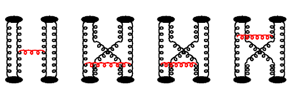
Figure 1: Diagrams representing the scattering amplitude $h_{fi}$ for glueball-glueball interaction with constituent gluon interchange.

3 The Constituent Gluon Model

3.1 The mass equation

In connection with the general formalism presented in the last section, we now concentrate in a particular microscopic model. The potential $V_{\rm aa}$ is chosen in the context of the Cornwall and Soni constituent gluon model (CGM) [10]. Their original work extended to study two-gluon and three-gluon glueballs. Gluon dynamics was described as massive spin-one fields interacting through massive spin-one exchange and by a breakable string. In the present we shall restrict our calculation to the two-gluon sector and total $L=0$. The CGM Hamiltonian is given by

$$H_{\rm aa}=2m-\frac{1}{m}\nabla^{2}+V_{\rm aa}$$ (12)

where $m$ is the effective gluon mass and

$$V_{\rm aa}(r)=\frac{1}{3}\,f^{ace}f^{bde}\left[\,V^{\rm OGEP}(r)+V_{S}(r)\right].$$ (13)

The potential $V_{\rm aa}$ in (13) contains a one-gluon exchange term $V^{\rm OGEP}$

$$V^{\rm OGEP}(r) = -\alpha\,\left[\,\omega_{1}\frac{e^{-mr}}{r}+\omega_{2}\frac{\pi}{m^{2}}\,F(r)\,\right]$$ (14)

where $\alpha=3\,\alpha_{s}$, $\omega_{1}$ and $\omega_{2}$ are defined as

$$\omega_{1} = \frac{1}{4}+\frac{1}{3}\vec{S}^{2}\,\,\,\,\,\,\,\,\,\,,\,\,\,\,\,\,\,\,\,\,\omega_{2}=1-\frac{5}{6}\vec{S}^{2}$$ (15)

with $\vec{S}$ is the glueball’s total spin. In (14) there appears a form factor $F(r)$, which beside the explicitly considered interactions parametrizes a residual interaction. This additional contribution is necessary to avoid a collapse of the glueball $0^{++}\/$ state and is set to be a Gaussian type with parameter $\rho$

$$F(r) = \frac{\rho^{3}}{\pi^{3/2}}\,e^{-\rho^{2}r^{2}}.$$ (16)

The second term in (13) is the string potential responsible for the confinement

$$V_{S}(r) = 2m\,(1-e^{-\beta\,m\,r})$$ (17)

where $\beta$ is the string tension.

The scattering amplitude is central in the calculation and shall depend on the parameters that appear in $V_{\rm aa}$, namely $\alpha$, $\beta$, $m$, $\rho$. A criterion for adjusting these parameters is that the expectation value of $H_{\rm aa}$ should render the glueball’s mass

$$\Phi_{\alpha}^{\ast\mu\nu}H_{\rm aa}(\mu\nu;\sigma\rho)\Phi_{\beta}^{\sigma\rho}=M_{G}.$$ (18)

The glueball’s wave-function $\Phi$ is written as a product

$$\Phi_{\alpha}^{\mu\nu}=\chi_{A_{\alpha}}^{s_{\mu}s_{\nu}}\,{\cal C}^{c_{\mu}c_{\nu}}\,\Phi_{\vec{P}_{\alpha}}^{\,\vec{p}_{\mu}\vec{p}_{\nu}},$$ (19)

$\chi_{A_{\alpha}}^{s_{\mu}s_{\nu}}$ is the spin contribution, with $A_{\alpha}\equiv\{S_{\alpha},S^{3}_{\alpha}\}$, where $S_{\alpha}$ is the glueball’s total spin index and $S^{3}_{\alpha}$ the index of the spin’s third component; ${\cal C}^{c_{\mu}c_{\nu}}$ is the color component given by

$${\cal C}^{c_{\mu}c_{\nu}}=\frac{1}{\sqrt{8}}\,\delta^{c_{\mu}c_{\nu}}$$ (20)

and the spatial wave-function is

$$\Phi_{\vec{P}_{\alpha}}^{\vec{p}_{\mu}\vec{p}_{\nu}}=\delta^{(3)}(\vec{P}_{\alpha}-\vec{p}_{\mu}-\vec{p}_{\nu})\,\phi(\vec{p}_{\mu}-\vec{p}_{\nu})\;,$$ (21)

where

$$\phi(\vec{p}_{\mu}-\vec{p}_{\nu})={\left(\frac{1}{\pi b^{2}}\right)}^{\frac{3}{4}}e^{-\frac{1}{8b^{2}}{\left(\vec{p}_{\mu}-\vec{p}_{\nu}\right)}^{2}}.$$ (22)

The expectation value of $r^{2}$ gives a relation between the $rms$ radius $r_{0}$ and $b$

$$b=\frac{\sqrt{1.5}}{r_{0}}.$$ (23)

These relations when introduced in (18) result in the mass equation which relates all parameters in the model

$$M_{G} = 4m+\frac{3b^{2}}{2m}-\frac{\omega_{1}\alpha}{\sqrt{\pi}}\left[2b+m\,\sqrt{\pi}\,e^{\frac{m^{2}}{4b^{2}}}\,{\rm erfc}{\left(\frac{m}{2b}\right)}\right]$$ (24)

$$-\frac{m\zeta^{3}\omega_{2}\alpha}{\sqrt{\pi}}\,\,\,\frac{b^{3}}{(b^{2}+\zeta^{2}m^{2})^{3/2}}+\frac{m}{\sqrt{\pi}b^{2}}\left[2b\beta m\frac{}{}\right.$$

$$\left.+\sqrt{\pi}\,e^{\frac{\beta^{2}m^{2}}{4b^{2}}}(2b^{2}+\beta^{2}m^{2})\,{\rm erfc}{\left(\frac{\beta m}{2b}\right)}\right]$$

where $\zeta=\rho/m$. The complementary error function is ${\rm erfc}(x)\equiv{\rm erf}(x)-1$ with

$${\rm erf}(x)=\frac{2}{\sqrt{\pi}}\int_{0}^{x}dt\,\,e^{-t^{2}}.$$ (25)

To adjust the parameters $\rho$ and $\beta$ without ambiguity we shall use the mass equation not only for $0^{++}$ but also for the next low-lying glueball candidate, in the $\vec{L}=0$ sector, the $2^{++}$ resonance. The results obtained from lattice QCD, for these resonances give a mass estimate for $M_{0^{++}}\approx 1.7$ GeV and $M_{2^{++}}\approx 2.4$ GeV. An additional result from lattice is that independent from the absolute mass values, the mass ratio shall be

$$\frac{M_{2^{++}}}{M_{0^{++}}}\simeq 1.4.$$ (26)

The model parameters were fixed using a parametric inference method reported in detail elsewhere [19], in order to calibrate the model for subsequent cross-section calculations. To this end we used a Likelihood Monte Carlo method that simultaneously fixed the parameters for the $0^{++}\/$ and the $2^{++}\/$ candidates. The following restrictions for the parameters were implemented: The string tension $\beta\/$ shall be common for both states since they shall appear in the same spectrum. The parameter $b\/$ for either state shall be of comparable magnitude, also the form-factor parameter $\zeta\/$ shall be comparable. The effective gluon mass shall be roughly an order of magnitude smaller than the glueball state [12, 13]. The glueball masses $M_{G}\/$ for the quantum numbers $0^{++}\/$ and $2^{++}\/$ shall be in the expected mass ranges given by Lattice calculations.

Maximizing the combined likelihood function for both states yielded the best parameter sets for both sates simultaneously. All parameters except for the glueball masses were generated randomly within a given interval and using an initially homogeneous distribution. The parameter combinations were accepted in a two step evaluation, first their glueball masses were to fit in an interval with a width $10\%\/$ of the respective glueball mass around the value determined from lattice QCD calculations. In a subsequent step, parameter combinations were excluded where the radius values $b(0^{++})\/$ and $b(2^{++})\/$ differed by more than a factor of two. From $10^{5}\/$ generated parameter combinations approximately half the number were accepted by the Likelihood criterion, fitting the two states in the same spectrum. The simultaneous glueball mass selection reduced the set to $14\/$ candidates from which three survived the elimination from the $b\/$ and $\zeta\/$ value differences of the respective $0^{++}\/$ and $2^{++}\/$ glueball states. The table 1 shows the three accepted parameter sets.

The gluon coupling constant $\alpha$ is three times larger than the strong coupling constant $\alpha_{s}$. The usual values for $\alpha_{s}$ is the order of $0.6$, which sets $\alpha$ to $1.8$. From the $rms$ radius $r_{0}$ relation to the wave-function’s $b$ parameter, Eq. (23), the usual hadronic range is reproduced with $r_{0}\approx 0.1-0.8fm\/$.

Table 1: Parameter sets for glueball candidates with $m\/$, $b\/$ and $M\/$ in units of $GeV\/$.

Set	$\beta$	$m$	$b(0^{++})$	$b(2^{++})$	$\zeta(0^{++})$	$\zeta(2^{++})$	$M(0^{++})$	$M(2^{++})$
(a)	$1.7$	$0.1$	$0.4$	$0.5$	$0.2$	$0.2$	$1.9$	$2.3$
(b)	$5.8$	$0.1$	$0.3$	$0.5$	$0.2$	$0.2$	$2.0$	$2.4$
(c)	$2.2$	$0.1$	$0.4$	$0.6$	$0.2$	$0.2$	$1.8$	$2.4$

3.2 The scattering amplitude and cross-section

In order to evaluate the cross-section given by equation (11) one has to obtain the scattering amplitude $h_{fi}$ from diagrams of figure 1. These diagrams are explicitly calculated as multidimensional integrals in the momentum space from Eqs. (8)-(10). The choice of a Gaussian wave-function for the spatial part of $\Phi$ in (22), provides a simplification in the integration and retains the basic ingredients of color confinement. Schematically the evaluation of the scattering amplitude can be written as the following product

$$h_{fi}(s,t)=\sum_{i}{\cal C}_{i}\,h_{i}(s,t,\omega_{1}^{(i)},\omega_{2}^{(i)})$$ (27)

Details of the spatial, color and spin factors calculation are presented in the appendix. Here we present the final result

$$h_{fi}(s,t) = \frac{3}{8}\,R_{0}(s)\sum_{i=1}^{6}\,R_{i}(s,t)$$ (28)

where

$$R_{0} = \frac{4}{(2\pi)^{3/2}b^{3}}\exp\left[-\frac{1}{2b^{2}}\left(\frac{s}{4}-M_{G}^{2}\right)\right]$$

$$R_{1} = \frac{\alpha\,\omega_{1}^{(2)}\,4\,\sqrt{2\pi}}{3}\,\,\int_{0}^{\infty}dq\,\frac{q^{2}}{q^{2}+m^{2}}\exp\left(-\frac{q^{2}}{2b^{2}}\right)$$

$$\times\left[{\mathcal{J}}_{0}\left(\frac{q\sqrt{t}}{2b^{2}}\right)+{\mathcal{J}}_{0}\left(\frac{q\sqrt{u}}{2b^{2}}\right)\right]$$

$$R_{2} = \frac{\alpha\,\omega_{2}^{(2)}2\sqrt{2}\pi b^{3}\zeta^{3}m}{3(b^{2}+2\zeta^{2}m^{2})^{3/2}}\left[\exp\left(-\frac{t\zeta^{2}m^{2}}{4(b^{4}+2b^{2}\zeta^{2}m^{2})}\right)\right.$$

$$+\left.\exp\left(-\frac{u\zeta^{2}m^{2}}{4(b^{4}+2b^{2}\zeta^{2}m^{2})}\right)\right]$$

$$R_{3} = \frac{32\sqrt{2\pi}}{3}\int_{0}^{\infty}dq\,\frac{q^{2}\beta m^{2}}{(q^{2}+\beta^{2}m^{2})^{2}}\exp\left(-\frac{q^{2}}{2b^{2}}\right)$$

$$\times\left[{\mathcal{J}}_{0}\left(\frac{q\sqrt{t}}{2b^{2}}\right)+{\mathcal{J}}_{0}\left(\frac{q\sqrt{u}}{2b^{2}}\right)\right]$$

$$R_{4} = -\frac{16\alpha\,\omega_{1}^{(3)}\sqrt{2\pi}\,b^{2}}{3\sqrt{\frac{s}{4}-M_{G}^{2}}}\int_{0}^{\infty}dq\,\frac{q}{q^{2}+m^{2}}$$

$$\times\exp\left(-\frac{3q^{2}}{8b^{2}}\right)\sinh\left(\frac{q}{2b^{2}}\sqrt{\frac{s}{4}-M_{G}^{2}}\,\right)$$

$$R_{5} = -\frac{16\alpha\,\omega_{2}^{(3)}\pi b^{3}\zeta^{3}m}{3(2b^{2}+3\zeta^{2}m^{2})^{3/2}}\exp\left[-\frac{\zeta^{2}m^{2}\left(\frac{s}{4}-M_{G}^{2}\right)}{2(2b^{4}+3b^{2}\zeta^{2}m^{2})}\right]$$

$$R_{6} = -\frac{128\sqrt{2\pi}b^{2}}{3\sqrt{\frac{s}{4}-M_{G}^{2}}}\int_{0}^{\infty}dq\,\frac{q\beta m^{2}}{(q^{2}+\beta^{2}m^{2})^{2}}$$ (29)

$$\times\exp\left(\frac{3q^{2}}{8b^{2}}\right)\sinh\left(\frac{q}{2b^{2}}\sqrt{\frac{s}{4}-M_{G}^{2}}\,\right).$$

In (29), ${\cal J}_{0}$ represents the spherical Bessel function defined by ${\cal J}_{0}(x)=\sin x/x$. The notation $\omega^{(i)}_{1}$ and $\omega^{(i)}_{2}$ is introduced, where the index $i$ corresponds to the number of the evaluated diagram in figure 1. The cross-section for scattering of the glueballs with constituent gluon interchange is obtained numerically by inserting Eqs. (28) and (29) in (11). Assigning values as determined from parametric inference to $M_{G}$ in order to correspond to the glueball $0^{++}$ ($M_{G}\approx 1.8-2.0$ GeV) and $2^{++}$ ($M_{G}\approx 2.3-2.4$ GeV) one obtains the energy dependence of the elastic scattering cross-sections (see graphs in figure 2).

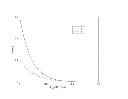
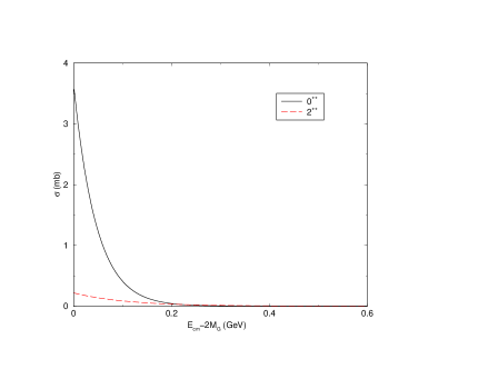
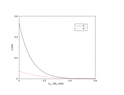
Figure 2: Elastic cross-section for three parameter sets, upper left $\beta=1.7\/$, $b(0^{++})=0.4\/$, $b(2^{++})=0.5\/$, $M(0^{++})=1.9\/$, $M(2^{++})=2.3\/$; upper right $\beta=5.8\/$, $b(0^{++})=0.3\/$, $b(2^{++})=0.5\/$, $M(0^{++})=2.0\/$, $M(2^{++})=2.4\/$ and lower $\beta=2.2\/$, $b(0^{++})=0.4\/$, $b(2^{++})=0.6\/$, $M(0^{++})=1.8\/$, $M(2^{++})=2.4\/$.

4 The Constituent Quark Model

In order to discuss meson-meson scattering with constituent quark interchange, one needs to specify the general form of the microscopic quark Hamiltonian. For our purposes here, the microscopic Hamiltonian can be written in terms of the quark and antiquark operators as

$$H = T(\mu)\;q_{\mu}^{\dagger}q_{\mu}+T(\mu)\;\bar{q}_{\mu}^{\dagger}\bar{q}_{\mu}+\frac{1}{2}V_{qq}(\mu\nu;\sigma\rho)\;q_{\mu}^{\dagger}q_{\nu}^{\dagger}q_{\rho}q_{\sigma}$$ (30)

$$+ \frac{1}{2}V_{\bar{q}\bar{q}}(\mu\nu;\sigma\rho)\bar{q}_{\mu}^{\dagger}\bar{q}_{\nu}^{\dagger}\bar{q}_{\rho}\bar{q}_{\sigma}+V_{q\bar{q}}(\mu\nu;\sigma\rho)q_{\mu}^{\dagger}\bar{q}_{\nu}^{\dagger}\bar{q}_{\rho}q_{\sigma}$$

where $T$ is the kinetic energy; $V_{qq}$, $V_{\bar{q}\bar{q}}$, $V_{q\bar{q}}$ are the quark-quark, antiquark-antiquark and quark-antiquark interactions. In our calculation we shall use, for $V_{qq}$ , the spin-spin hyperfine component of the perturbative one gluon interaction

$$V_{qq}=-\,\frac{8\pi\alpha_{s}}{3\,m_{i}m_{j}}\,{\bf S}_{i}\cdot{\bf S}_{j}\,\,\,{\cal F}^{\,a}_{i}\,\,{\cal F}^{\,a}_{j}\,\,\,,$$ (31)

where ${\cal F}^{\,a}_{i}=\lambda^{a}_{i}/2$ are the Gell-Mann matrices. To obtain $V_{\bar{q}\bar{q}}$, one substitutes $\lambda\rightarrow-\lambda^{T}$ and for $V_{q\bar{q}}$ the following $\lambda_{j}\rightarrow-\lambda^{T}_{j}$ in (31).

There is a considerable literature related to free meson-meson and baryon-baryon scattering with constituent interchange [20] - [30]. In many of these models the potential is much more elaborated than (31) (including Coulomb, spin-orbit, tensor, confinement terms and eventually meson coupling to quarks). The lesson taken from all of these approaches is that the dominant term for the short-range repulsion is basically the spin-spin term from the one gluon exchange potential. Its strong influence is seen, for example, in the ${}^{1}S_{\,0}$ partial-wave.

The Fock-Tani formalism has been used in this context to study heavy meson scattering by pions as described in reference [17] and [18]. The scattering amplitude obtained is represented in figure 3. The corresponding cross-section for a $0^{++}$ meson with a $s\bar{s}$ content can be derived directly from this previous result by a simple substitutions: the quark’s mass $m_{q}\rightarrow m_{s}$ and the meson’s mass by the glueballs $M\rightarrow M_{G}\/$. The remaining coefficients are unchanged. As described in [17] the meson wave-function is Gaussian which implies exact analytical results for the scattering amplitude

$$h_{fi}^{(s\bar{s})-(s\bar{s})} = \frac{8\pi\alpha_{s}}{9m^{2}_{s}(2\pi)^{3}}\left[\frac{16}{3\sqrt{3}}e^{-\frac{\xi}{12b^{2}}}+e^{\frac{t}{8b^{2}}}+e^{-\frac{u}{8b^{2}}}\right]$$

with $\xi=s-4M_{G}^{2}$. The parameter $b$ has an equivalent origin as for the glueball, it is the Gaussian length parameter and is related to the meson’s rms radius $r_{0}$ by the same expression as before: Eq. (23). The cross-section is obtained inserting Eq. (LABEL:hfi-ss) in (11) which results in

$$\sigma^{(s\bar{s})-(s\bar{s})} = \frac{4\pi\alpha_{s}^{2}s}{81m_{s}^{4}}\left[\frac{4b^{2}\left(1-e^{-\frac{\xi}{4b^{2}}}\right)}{\xi}+\frac{128}{27}e^{-\frac{\xi}{6b^{2}}}\right.$$

$$\left.+e^{-\frac{\xi}{8b^{2}}}+\frac{64}{3\sqrt{3}}\frac{4b^{2}}{\xi}\left(e^{-\frac{\xi}{12b^{2}}}-e^{-\frac{5\xi}{24b^{2}}}\right)\right]\;$$

The comparison between the cross-sections in the glueball picture and the quark picture for the $0^{++}$ meson is given in figure 4. There is a sensitive difference in the cross-sections as a function of their internal structure. For low energies it is a notable that the quark-$0^{++}$ reaches high vales, while the gluon-$0^{++}$ approaches zero. For higher CM energies the curves have a similar behavior, even though the $rms$ have different values. The same comparison for the $2^{++}$ is beyond the scope of the present work, which would imply in contributions with $\vec{L}\neq 0$ in order to build the correct angular momentum states.

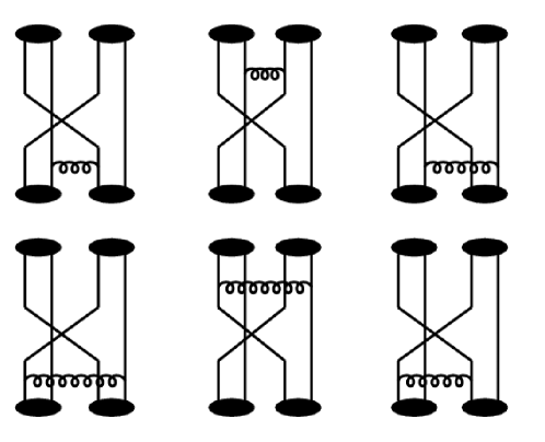
Figure 3: Diagrams representing the scattering amplitude $h_{fi}$ for meson-meson interaction with constituent quark interchange.

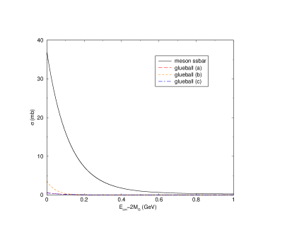
Figure 4: Cross-section comparison for $0^{++}$ states.

5 Conclusions

In the present article we compared two elastic scattering scenarios for the $0^{++}\/$ meson with mass $\sim 1.7$ GeV: one in which it was considered as a pure glueball and another as a $s\bar{s}\/$ state. No particular mixing scheme was introduced. A scattering cross-section for the $2^{++}\/$ $s\bar{s}$-meson, with mass $M\sim 2.4$ GeV, was also calculated. The same comparison for this case was beyond the scope of the present work, which would imply in contributions with $\vec{L}\neq 0$ in the CGM in order to build the correct angular momentum states.

The comparison, for the $0^{++}\/$ meson, showed that the glueball-glueball elastic scattering cross-section for a color singlet state from is between one to two orders of magnitude smaller than the corresponding $q\bar{q}\/$ state. The glueball-glueball cross-section for $2^{++}\/$ presented the same behavior. Thus, if added as a new channel to already existing modes in presently used transport codes like the UrQMD, glueball-glueball scattering is not very likely to introduce significant changes in, for example, the flow properties. Though, glue states whether pure or mixed are believed to somehow play a manifest role in collisions. However, there still might be a contribution from $q\bar{q}\/$-glue mixed states, once defined the particular mixing scheme, with correspondence in hadronic spectra. This effect which we shall investigate in a subsequent work.

If our result holds for other color singlet states containing pure glue, then it seems that states identified in hadron spectroscopy, with stronger evidence as glueball or glue rich states, do not contribute significantly to signatures in heavy ion reactions and one shall resort to new possibilities as already indicated by lattice calculations [7, 8], meaning that hadronic states known inside a hadronic environment with high density and temperature have no or almost no vacuum counter parts. Results from lattice calculations [7, 8] point towards a direction, where a number of new states shall be considered and tested whether they suit to explain the apparently low viscose flow property, which is considered a strong indication for QGP. At high temperatures bulk states of quarks, gluons and mixed states may exist and form quasi-particles [31], which might explain the almost perfect liquid property of the plasma.

Acknowledgments

The authors would like to thank H. Stöcker, J. Aichelin and W. Greiner for important and enlightening discussions at 2${}^{\rm\,nd}$ International Workshop on Astronomy and Relativistic Astrophysics (IWARA) held at Natal, R.N., Brazil, 2005.

Appendix A Evaluation of the color factor, spin matrices and spatial integrals for glueball-glueball interaction

The color factor ${\cal C}_{i}$, is calculated for each diagram of figure 1,

$${\cal C}_{1} = f^{\mu\sigma\lambda}f^{\nu\rho\lambda}\,\,{\cal C}^{\mu\tau}{\cal C}^{\nu\xi}{\cal C}^{\rho\xi}{\cal C}^{\sigma\tau}$$

$${\cal C}_{2} = f^{\mu\sigma\lambda}f^{\nu\rho\lambda}\,\,{\cal C}^{\mu\tau}{\cal C}^{\nu\xi}{\cal C}^{\rho\tau}{\cal C}^{\sigma\xi}$$

$${\cal C}_{3} = f^{\mu\sigma\lambda}f^{\nu\rho\lambda}\,\,{\cal C}^{\mu\nu}{\cal C}^{\tau\xi}{\cal C}^{\sigma\tau}{\cal C}^{\rho\xi}$$

$${\cal C}_{4} = f^{\mu\sigma\lambda}f^{\nu\rho\lambda}\,\,{\cal C}^{\mu\xi}{\cal C}^{\nu\tau}{\cal C}^{\tau\xi}{\cal C}^{\rho\sigma}.$$ (33)

In (20) is definition of the color wave-function which reduces (33) to

$${\cal C}_{1} = \frac{1}{64}f^{\mu\sigma\lambda}f^{\nu\rho\lambda}\,\,\delta^{\mu\tau}\delta^{\nu\xi}\delta^{\rho\xi}\delta^{\sigma\tau}$$

$${\cal C}_{2} = \frac{1}{64}f^{\mu\sigma\lambda}f^{\nu\rho\lambda}\,\,\delta^{\mu\tau}\delta^{\nu\xi}\delta^{\rho\tau}\delta^{\sigma\xi}$$

$${\cal C}_{3} = \frac{1}{64}f^{\mu\sigma\lambda}f^{\nu\rho\lambda}\,\,\delta^{\mu\nu}\delta^{\tau\xi}\delta^{\sigma\tau}\delta^{\rho\xi}$$

$${\cal C}_{4} = \frac{1}{64}f^{\mu\sigma\lambda}f^{\nu\rho\lambda}\,\,\delta^{\mu\xi}\delta^{\nu\tau}\delta^{\tau\xi}\delta^{\rho\sigma}$$ (34)

The quantities $f^{abc}$ are $SU(3)$ coefficients. After total contraction of the color indexes in (34) one finds

$${\cal C}_{1} = 0\,\,\,\,\,\,\,\,\,\,,\,\,\,\,\,\,\,\,\,\,{\cal C}_{2}=-\frac{3}{8}$$

$${\cal C}_{3} = \frac{3}{8}\,\,\,\,\,\,\,\,\,\,,\,\,\,\,\,\,\,\,\,\,{\cal C}_{4}=\frac{3}{8}.$$ (35)

The zero in ${\cal C}_{1}$ of (35) is an expected result as the consequence of exchanging a color object (gluon) between two white objects (glueballs)

The vector $\vec{S}$ is the glueball’s total spin which can be written in terms of the constituent gluon spin $\vec{S}_{1}$ e $\vec{S}_{2}$

$$\vec{S}^{2} = S_{1}^{2}+S_{2}^{2}+2\vec{S}_{1}\cdot\vec{S}_{2}\,\,.$$ (36)

Using the following quantum-mechanical property, for spin-one particles $\vec{S}_{i}^{2}=2$, eq. (36) can be written as

$$\vec{S}^{2}=4+2\vec{S}_{1}\cdot\vec{S}_{2}.$$ (37)

After the substitution of (37) in (15) one obtains

$$\omega_{1}(\mu\nu;\sigma\rho) = \frac{19}{12}\delta_{\mu\sigma}\delta_{\nu\rho}+\frac{2}{3}\vec{S}_{1\,\mu\sigma}\cdot\vec{S}_{2\,\nu\rho}$$ (38)

$$\omega_{2}(\mu\nu;\sigma\rho) = -\frac{7}{3}\delta_{\mu\sigma}\delta_{\nu\rho}-\frac{5}{3}\vec{S}_{1\,\mu\sigma}\cdot\vec{S}_{2\,\nu\rho}.$$ (39)

The spin contribution for each diagram is

$$\omega_{1}^{(1)} = \omega_{1}(\mu\nu;\sigma\rho)\,\chi^{\star\mu\tau}_{A_{\alpha}}\chi^{\star\nu\xi}_{A_{\gamma}}\chi^{\rho\xi}_{A_{\delta}}\chi^{\sigma\tau}_{A_{\beta}}$$

$$\omega_{1}^{(2)} = \omega_{1}(\mu\nu;\sigma\rho)\,\chi^{\star\mu\tau}_{A_{\alpha}}\chi^{\star\nu\xi}_{A_{\gamma}}\chi^{\rho\tau}_{A_{\delta}}\chi^{\sigma\xi}_{A_{\beta}}$$

$$\omega_{1}^{(3)} = \omega_{1}(\mu\nu;\sigma\rho)\,\chi^{\star\mu\nu}_{A_{\alpha}}\chi^{\star\tau\xi}_{A_{\gamma}}\chi^{\sigma\tau}_{A_{\delta}}\chi^{\rho\xi}_{A_{\beta}}$$

$$\omega_{1}^{(4)} = \omega_{1}(\mu\nu;\sigma\rho)\,\chi^{\star\mu\xi}_{A_{\alpha}}\chi^{\star\nu\tau}_{A_{\gamma}}\chi^{\tau\xi}_{A_{\delta}}\chi^{\rho\sigma}_{A_{\beta}}$$ (40)

and

$$\omega_{2}^{(1)} = \omega_{2}(\mu\nu;\sigma\rho)\,\chi^{\star\mu\tau}_{A_{\alpha}}\chi^{\star\nu\xi}_{A_{\gamma}}\chi^{\rho\xi}_{A_{\delta}}\chi^{\sigma\tau}_{A_{\beta}}$$

$$\omega_{2}^{(2)} = \omega_{2}(\mu\nu;\sigma\rho)\,\chi^{\star\mu\tau}_{A_{\alpha}}\chi^{\star\nu\xi}_{A_{\gamma}}\chi^{\rho\tau}_{A_{\delta}}\chi^{\sigma\xi}_{A_{\beta}}$$

$$\omega_{2}^{(3)} = \omega_{2}(\mu\nu;\sigma\rho)\,\chi^{\star\mu\nu}_{A_{\alpha}}\chi^{\star\tau\xi}_{A_{\gamma}}\chi^{\sigma\tau}_{A_{\delta}}\chi^{\rho\xi}_{A_{\beta}}$$

$$\omega_{2}^{(4)} = \omega_{2}(\mu\nu;\sigma\rho)\,\chi^{\star\mu\xi}_{A_{\alpha}}\chi^{\star\nu\tau}_{A_{\gamma}}\chi^{\tau\xi}_{A_{\delta}}\chi^{\rho\sigma}_{A_{\beta}}.$$ (41)

The glueball’s spin wave-function can be written in the following notation

$$|S,S^{3}\rangle_{\rm G}=\chi^{s_{1}s_{2}}_{S,S^{3}}|s_{1},s_{2}\rangle_{\rm g}\,\,.$$ (42)

The coupling of two spin-one particles $s_{1}$ and $s_{2}$ in a total angular momentum state of $\vec{S}=0$ or $\vec{S}=2$ can be written using angular momentum addition rules. In this sense for a state with $S=0$ and $S^{3}=0$ one has

$$|0,0\rangle_{\rm G}=\frac{1}{\sqrt{3}}\left[\,\frac{}{}|1,-1\rangle_{\rm g}-|0,0\rangle_{\rm g}+|-1,1\rangle_{\rm g}\,\right].$$ (43)

By comparison of state (42) with (43) one finds that

$$\chi^{1,-1}_{0,0}=\frac{1}{\sqrt{3}}\,\,\,\,\,\,,\,\,\,\,\,\,\chi^{0,0}_{0,0}=-\frac{1}{\sqrt{3}}\,\,\,\,\,\,,\,\,\,\,\,\ \chi^{-1,1}_{0,0}=\frac{1}{\sqrt{3}}.$$ (44)

The state with $S=2$ has five projections $S^{3}=$-2,-1,0,1,2 which yields

$$|2,2\rangle_{\rm G} = |1,1\rangle_{\rm g}$$

$$|2,1\rangle_{\rm G} = \frac{1}{\sqrt{2}}\left[\frac{}{}\,|1,0\rangle_{\rm g}+|0,1\rangle_{\rm g}\right]$$

$$|2,0\rangle_{\rm G} = \frac{1}{\sqrt{6}}|1,-1\rangle_{\rm g}+\sqrt{\frac{3}{2}}|\,0,0\rangle_{\rm g}+\frac{1}{\sqrt{6}}|-1,1\rangle_{\rm g}$$

$$|2,-1\rangle_{\rm G} = \frac{1}{\sqrt{2}}\left[\,\frac{}{}|1,0\rangle_{\rm g}+|0,1\rangle_{\rm g}\right]$$

$$|2,-2\rangle_{\rm G} = |-1,-1\rangle_{\rm g}\,.$$ (45)

By comparison of state (42) with (45) one finds that

$$\chi^{1,1}_{2,2} = 1$$

$$\chi^{1,0}_{2,0} = \frac{1}{\sqrt{2}}\,\,\,\,\,\,,\,\,\,\,\,\ \chi^{0,1}_{2,1}=\frac{1}{\sqrt{2}}$$

$$\chi^{1,-1}_{2,0} = \frac{1}{\sqrt{6}}\,\,\,\,\,\,,\,\,\,\,\,\,\chi^{0,0}_{2,0}=\sqrt{\frac{3}{2}}\,\,\,\,\,\,,\,\,\,\,\,\ \chi^{-1,1}_{2,0}=\frac{1}{\sqrt{6}}$$

$$\chi^{0,-1}_{2,-1} = \frac{1}{\sqrt{2}}\,\,\,\,\,\,,\,\,\,\,\,\ \chi^{-1,0}_{2,-1}=\frac{1}{\sqrt{2}}$$

$$\chi^{-1,-1}_{2,-2} = 1.$$ (46)

Using these definitions, after contraction, of the spin indexes one finds that for $S=0$

$$\omega_{1}^{(1)} = 1.58333326$$

$$\omega_{1}^{(2)} = 0.972222179$$

$$\omega_{1}^{(3)} = 0.675925895$$

$$\omega_{1}^{(4)} = 0.675925895$$ (47)

$$\omega_{2}^{(1)} = -2.33333309$$

$$\omega_{2}^{(2)} = -1.8888887$$

$$\omega_{2}^{(3)} = -1.14814803$$

$$\omega_{2}^{(4)} = -1.14814803\,.$$ (48)

For $S=2$, the present calculation considered the unpolarized cross-section which implies in performing an average over the spin states resulting in

$$\omega_{1}^{(1)} = 1.58333334$$

$$\omega_{1}^{(2)} = 1.46228344$$

$$\omega_{1}^{(3)} = 1.18539605$$

$$\omega_{1}^{(4)} = 1.18539605$$ (49)

$$\omega_{2}^{(1)} = -2.33333321$$

$$\omega_{2}^{(2)} = -2.24529693$$

$$\omega_{2}^{(3)} = -1.55307847$$

$$\omega_{2}^{(4)} = -1.55307847\,.$$ (50)

The evaluation of the spatial part of the amplitude $h_{fi}$ is performed in the momentum space, where the scattering is described in the center of mass with the CM variables: $(\vec{p},\vec{p}^{\,{}^{\prime}})$. The OGEP has the following property

$$V_{\rm aa}(\vec{p})=V_{\rm aa}(-\vec{p}).$$ (51)

In this form the spatial contribution for each diagram of figure 1 is obtained

$$h_{1}(\vec{p},\vec{p}^{\,{}^{\prime}},\omega_{1}^{(1)},\omega_{2}^{(1)})=4\,V_{\rm aa}(\vec{p}-\vec{p}^{\,\prime})\exp\left[-\frac{(\vec{p}-\vec{p}^{\,\prime})^{2}}{8b^{2}}\right]$$

$$+4V_{\rm aa}(\vec{p}+\vec{p}^{\prime})\exp\left[-\frac{(\vec{p}+\vec{p}^{\prime})^{2}}{8b^{2}}\right]$$

$$h_{2}(\vec{p},\vec{p}^{\,{}^{\prime}},\omega_{1}^{(2)},\omega_{2}^{(2)})=\frac{4}{(2\pi)^{3/2}b^{3}}\exp\left[-\frac{(p^{2}+p^{\prime 2})}{4b^{2}}\right]$$

$$\times\int d\vec{q}\,V_{\rm aa}(\vec{q})\left\{\exp\left[-\frac{q^{2}}{2b^{2}}-\frac{q\cdot(\vec{p}-\vec{p}^{\,\prime})}{2b^{2}}\right]\right.$$

$$\left.+\exp\left[-\frac{q^{2}}{2b^{2}}-\frac{q\cdot(\vec{p}+\vec{p}^{\,\prime})}{2b^{2}}\right]\right\}$$

$$h_{3}(\vec{p},\vec{p}^{\,{}^{\prime}},\omega_{1}^{(3)},\omega_{2}^{(3)})=\frac{4}{(2\pi)^{3/2}b^{3}}\exp\left[-\frac{(p^{2}+p^{\prime 2})}{4b^{2}}\right]$$

$$\times\int d\vec{q}\,V_{\rm aa}(\vec{q})\left\{\exp\left[-\frac{3q^{2}}{8b^{2}}+\frac{\vec{q}\cdot\vec{p}^{\,\prime}}{2b^{2}}\right]\right.$$

$$+\left.\exp\left[-\frac{3q^{2}}{8b^{2}}+\frac{\vec{q}\cdot\vec{p}}{2b^{2}}\right]\right\}$$

$$h_{4}(\vec{p},\vec{p}^{\,{}^{\prime}},\omega_{1}^{(4)},\omega_{2}^{(4)})=\frac{4}{(2\pi)^{3/2}b^{3}}\exp\left[-\frac{(p^{2}+p^{\prime 2})}{4b^{2}}\right]$$

$$\times\int d\vec{q}\,V_{\rm aa}(\vec{q})\left\{\exp\left[-\frac{3q^{2}}{8b^{2}}+\frac{\vec{q}\cdot\vec{p}^{\,\prime}}{2b^{2}}\right]\right.$$

$$\left.+\exp\left[-\frac{3q^{2}}{8b^{2}}+\frac{\vec{q}\cdot\vec{p}}{2b^{2}}\right]\right\}\,.$$ (52)

The final form for the scattering amplitude is written as

$$h_{fi}(\vec{p},\vec{p}^{\,{}^{\prime}})=\sum_{i=1}^{4}{\cal C}_{i}\,h_{i}(\vec{p},\vec{p}^{\,{}^{\prime}},\omega_{1}^{(i)},\omega_{2}^{(i)})\,,$$ (53)

from space, color and spin calculation one finds

$${\cal C}_{1} = 0\,\,\,\,\,\,\,\,\,,\,\,\,\,\,\,\,\,\,{\cal C}_{3}={\cal C}_{4}$$

$$\omega_{i}^{(3)} = \omega_{i}^{(4)}\,\,\,\,\,\,\,\,\,,\,\,\,\,\,\,\,\,\,h_{3}=h_{4}$$ (54)

which results

$$h_{fi}(\vec{p},\vec{p}^{\,\prime})={\cal C}_{2}\,h_{2}(\vec{p},\vec{p}^{\,\prime},\omega_{1}^{(2)},\omega_{2}^{(2)})+2\,{\cal C}_{3}\,h_{3}(\vec{p},\vec{p}^{\,\prime},\omega_{1}^{(3)},\omega_{2}^{(3)})\,,$$ (55)

or written in terms of the Mandelstam variables $(s,t)$

$$h_{fi}(s,t)={\cal C}_{2}\,h_{2}(s,t,\omega_{1}^{(2)},\omega_{2}^{(2)})+2\,{\cal C}_{3}\,h_{3}(s,t,\omega_{1}^{(3)},\omega_{2}^{(3)})\,.$$ (56)

References

References

- [1] Fritsch H, Minkowski P 1975 Nuov. Cim. 30A 393.
- [2] Vento V 2005 arXiv:nucl-th/0509102.
- [3] Amsler C and Close F E 1995 Phys. Lett. B353 385.
- [4] Amsler C and Close F E 1996 Phys. Rev. D53 295.
- [5] Thoma U 2003 Eur. Phys. J. A18 135.
- [6] Barberis D. et al. 2000 Phys. Lett. B479 345.
- [7] Morningstar C J and Peardon M, 1999 Phys. Rev. D60 034509.
- [8] Bali G et al. (UKQCD) 1993Phys. Lett. B309 378.
- [9] —–2000 Phys. Rev. D62 054503.
- [10] Cornwall J M and Soni A 1983 Phys. Lett. B120 431.
- [11] Hou W S and Soni A 1984 Phys. Rev. D29 101.
- [12] Hou W S, Luo C S and Wong G G 2001 Phys. Rev. D64 014028.
- [13] Hou W S and Wong G G 2003 Phys. Rev. D67 034003.
- [14] Huang H G 2001 hep-ex/0104024
- [15] Bai J Z et al 2003 hep/ex/0307058
- [16] Close F E and Kirk A 2001 Eur. Phys. J. C21 531.
- [17] Hadjimichef D, Krein G, Szpigel S and da Veiga J S 1998 Ann. of Phys. 268 105.
- [18] Szpigel S 1995 Interação Méson-Méson no Formalismo Fock-Tani. PhD thesis (Doutorado em Ciências) - Instituto de Física, Universidade de São Paulo, São Paulo.
- [19] da Silva M L L , Hadjimichef D, Bodmann B E J 2005 article in preparation.
- [20] Oka M and Yazaki K 1981 Prog. Theor. Phys. 66 556.
- [21] Oka M and Yazaki K 1981 Prog. Theor. Phys. 66 572.
- [22] Swanson E S 1992 Ann. of Phys. 220 73.
- [23] Barnes T and Swanson E S 1992 Phys. Rev. D46 131.
- [24] Barnes T, Capstick S, Kovarik M D and Swanson E S 1993 Phys. Rev. C48 539.
- [25] Hadjimichef D, Krein G, Szpigel S and da Veiga J S 1996 Phys. Lett. B367 317.
- [26] Wu G H, Teng L J, Ping J L, Wang F, Goldman T, 1996 Phys. Rev. C53 1161.
- [27] Ping J L, Wang F, Goldman T 1999 Nucl. Phys. A657 95.
- [28] Hadjimichef D, Haidenbauer J, Krein G 2001 Phys. Rev. C63 035204; e-Print Archive: nucl-th/0010044.
- [29] Hadjimichef D, Haidenbauer J, Krein G 2002 Phys. Rev. C66 055214.
- [30] da Silva D T , Hadjimichef D, 2004 J. Phys. G30 191.
- [31] Hansen T H, Wirstam J, Zahed I, 1998 Phys. Rev. D58 065012 .