Pentaquark state in pole-dominated QCD sum rules

Abstract

We propose a new approach in QCD sum rules applied for exotic hadrons with a number of quarks, exemplifying the pentaquark $\Theta^{+}(I=0,J=1/2)$ in the Borel sum rule. Our approach enables reliable extraction of the pentaquark properties from the sum rule with good stability in a remarkably wide Borel window. The appearance of its valid window originates from a favorable setup of the correlation functions with the aid of chirality of the interpolating fields on the analogy of the Weinberg sum rule for the vector currents. Our setup leads to large suppression of the continuum contributions which have spoiled the Borel stability in the previous analyses, and consequently enhances importance of the higher-dimensional contributions of the OPE, which are indispensable for investigating the pentaquark properties. Implementing the OPE analysis up to dimension 15, we find that the sum rules for the chiral-even and odd parts independently give the $\Theta^{+}$ mass of $1.68\pm 0.22$ GeV with uncertainties of the condensate values. Our sum rule indeed gives rather flat Borel curves almost independent of the continuum thresholds both for the mass and pole residue. Finally, we also discuss possible isolation of the observed states from the $KN$ scattering state on view of chiral symmetry.

I Introduction

The first discovery of the baryonic resonance with $S=1$, $\Theta^{+}(1540)$, and its confirmation in subsequent low-energy exclusive experiments in 2003 exp triggered tremendous amount of theoretical works on exotic hadrons in a short time. Many of their studies have been devoted to clarifying mainly its possible structure and its property such as spin and parity, and further searching for other exotic states theo ; JW . So far, it is experimentally known that the $\Theta^{+}$ has minimal quark contents, $uudd\bar{s}$, from observation of its decay mode into $KN$, with $I_{3}=0$ and most likely an isospin singlet $I=0$ exprev .

Yet the experimental evidence for the existence of $\Theta^{+}$ is not so obvious. While new data with better statistics from the LEPS collaboration consolidate their positive evidence of the $\Theta^{+}$ leps , the most recent experiment in low-energy exclusive reaction with high statistics by the CLAS Collaboration clas , however, showed negative evidence for the $\Theta^{+}$, suggesting that their previous result would be just a statistical fluctuation. The inclusive high-energy processes in $e^{+}e^{-}$ or hadron collisions have also claimed no evidence high_energy . The disagreement between the LEPS and the other experiments would possibly originate from their differences of experimental setup and kinematical conditions; the former experiment covers well the forward angle, where the $\Theta^{+}$ would be produced by meson-exchange production mechanism at low energy.

Theoretical study on existence of the $\Theta^{+}$ is also a very important issue. Investigation of such an exotic hadron can be the first step to explore the quark matter. To identify the exotic state definitely, theoretical computations in direct approaches of QCD with less assumptions and better accuracy are getting more important. One of its possible analyses is the QCD sum rule (QSR) shifman , which is a powerful tool to address directly nonperturbative dynamics peculiar to QCD as well as lattice QCD and is a quite established approach for reproducing the baryon masses IoffeN including their resonance states Jido .

Indeed, a number of the QSR analyses for scrutinizing the $\Theta^{+}$ mass were implemented with the help of the Borel sum rules (BSR’s) SDO ; bsr ; Oga and the finite energy sum rules fesr . It is generally known that the former technique is superior to the latter quantitatively, because in the former the highly excited states can be controlled by the inverse Borel mass ($1/M$) to isolate the desired pole contribution. To the best of our knowledge, so far no BSR analyses for the $\Theta^{+}$ mass have focused upon desirable pole-dominance of the $\Theta^{+}$, even accounting for higher corrections of the operator product expansion (OPE). But rather they have stuck with an undesirable continuum dominant region, so that they could not establish valid Borel windows. The work in Ref. fesr has closely viewed this problem and indeed they gave up relying on the Borel technique.

Our main objective of this paper is to put forward a solution to the problem in the BSR, by illustrating the $I=0$ and $J=1/2$ case of the $\Theta^{+}$, in a general way for exotic hadrons beyond the BSR. We here summarize the essential points of our analysis: (I) In order to incorporate low-energy contributions more into our analysis, we take into account the higher-dimensional terms of the OPE up to dimension 15. (II) Through a favorable linear combination of correlation functions, we suppress the high-energy continuum contamination with the aid of the chiral symmetry in analogy of the Weinberg sum rule. These technical developments enable us to establish Borel window wide enough to investigate the low energy hadronic properties of the resonance and scattering states.

This paper is organized as follows. In Sec. II, we briefly review the basic concepts of QSR’s with special emphasis on the importance of the pole dominance and the higher order terms in the OPE, discussing the problems in the previous works. In Sec. III, to overcome the problems in previous works, we introduce a linear combination of the correlation functions with the aim of suppressing the continuum contamination, in which chiral symmetry plays an important role in this cancellation. We also discuss calculation of the OPE and show all the OPE terms used in our analysis. In Sec. IV, we show our Borel analysis focusing on the criterion to set up the Borel window. We confirm the pole dominance and the OPE convergence. The values of the $\Theta^{+}$ mass and residue obtained in this analysis are also shown. Sec. V is devoted to a brief discussion on the $KN$ scattering states and on relation between experimental observation and our correlation function analysis. Finally we summarize this work in Sec. VI.

II The basic concepts of QSR and problems in the previous works

Following the standard way of the QCD sum rule, we start with the time-ordered two-point correlation function defined by

$$i\int d^{4}xe^{iq\cdot x}\langle 0|T[J(x)\bar{J}(0)]|0\rangle=\hat{q}\Pi_{0}(q^{2})+\Pi_{1}(q^{2}),$$ (1)

where $\hat{q}\equiv q^{\mu}\gamma_{\mu}$ and $\Pi_{0,1}(q^{2})$ are called the chiral-even and odd parts, respectively. Here $\langle 0|\cdots|0\rangle$ denotes a vacuum expectation value (hereafter for brevity $\langle\cdots\rangle$). The interpolating field $J(x)$ for the $\Theta^{+}$ consists of five quark fields with its quantum number. The QSR is then obtained through the dispersion relation,

$${\rm Re}\Pi_{i}(q^{2})=P\int_{0}^{\infty}ds\,[{\rm Im}\Pi_{i}(s)/\pi]/(s-q^{2})$$ (2)

for $i=0,1$. ${\rm Im}\Pi_{i}(s)$ satisfies the spectral conditions,

$${\rm Im}\Pi_{0}(s)\geq 0,\ \sqrt{s}{\rm Im}\Pi_{0}(s)-{\rm Im}\Pi_{1}(s)\geq 0.$$ (3)

For sufficiently large $-q^{2}$, the left hand side of (2) can be expressed by the OPE with products $C_{i}$ of the Wilson coefficients and the vacuum condensates:

$$\Pi_{i}^{ope}(q^{2})=\sum_{j=0}^{5}C_{2j+i}\ (q^{2})^{5-j}\log(-q^{2})+\sum_{j=1}^{\infty}\frac{C_{10+2j+i}}{(q^{2})^{j}}.\,$$ (4)

The OPE starts from $(q^{2})^{5}\log(-q^{2})$ reflecting the large number of quark fields in the $\Theta^{+}$ interpolating field.

The imaginary part in the right hand side of (2) is parameterized as the hadronic spectrum. We use the conventional pole plus continuum spectrum with a single $\Theta^{+}$ resonance:

$${\rm Im}\Pi_{i}^{h}(s)\simeq\pi\lambda_{i}^{2}\delta(s-m_{\Theta^{+}}^{2})+\theta(s-s_{th}){\rm Im}\Pi_{i}^{ope}(s).$$ (5)

Here $m_{\Theta^{+}}$ denotes the $\Theta^{+}$ mass, and the residue $\lambda_{i}$ is the coupling strength of interpolating field to the resonance, satisfying

$$\pm m_{\Theta^{+}}\lambda_{0}^{2}=\lambda_{1}^{2}$$ (6)

for parity $\pm 1$ respectively. The second term represents a model of continuum contribution with its threshold $s_{th}$ based on the simple duality ansatz. The QSR (2) gives the physical quantities ($m_{\Theta^{+}}$, $\lambda_{i}$) in terms of the known QCD parameters appearing in Eq. (4) shifman .

Our QSR’s are obtained from Eqs. (2) and (4) for the chiral even and odd parts independently, by using the Borel transformation technique reinders , which qualitatively improves isolation of the $\Theta^{+}$ pole:

$$\lambda_{i}^{2}e^{-m_{\Theta^{+}}^{2}/M^{2}}=\sum_{j=1}^{\infty}\frac{(-)^{j}}{\Gamma(j)}\ \frac{C_{10+2j+i}}{(M^{2})^{j-1}}$$ (7)

$$+\left(\int_{0}^{\infty}-\int_{s_{th}}^{\infty}\right)ds\,e^{-s/M^{2}}\sum_{j=0}^{5}C_{2j+i}\ s^{5-j}$$

where the continuum term in the hadronic spectrum is transferred to the second integral in the right hand side using the duality ansatz. It is worth noting here that, in this ansatz, the continuum term is expressed in terms of the logarithmic terms in Eq. (4) and it appears in the Borel sum rules (7) as the integral of $\exp(-s/M^{2})$ weighted by polynomials of $s$. For later convenience, we define

$$A_{i}(M^{2};s_{th}) = \int^{s_{th}}_{0}\!\!ds\ e^{-s/M^{2}}\frac{1}{\pi}{\rm Im}\Pi_{i}^{ope}(s)$$ (8)

$$= \sum_{j=1}^{\infty}\frac{(-)^{j}}{\Gamma(j)}\ \frac{C_{10+2j+i}}{(M^{2})^{j-1}}$$

$$+\int_{0}^{s_{th}}ds\,e^{-s/M^{2}}\sum_{j=0}^{5}C_{2j+i}\ s^{5-j}\ ,$$

$$B_{i}(M^{2};s_{th}) \equiv \int_{s_{th}}^{\infty}\!\!ds\ e^{-s/M^{2}}\frac{1}{\pi}{\rm Im}\Pi_{i}^{ope}(s)$$ (9)

$$= \int_{s_{th}}^{\infty}\!\!ds\ e^{-s/M^{2}}\sum_{j=0}^{5}C_{2j+i}\ s^{5-j}.$$

$A_{i}(M^{2};s_{th})$ is equal to the right hand side of Eq. (7). These functions give portions of the Borel integration of $\Pi_{i}^{ope}$ for given threshold $s_{th}$.

In the pole-plus-continuum ansatz, the threshold $s_{th}$ is very important parameter. It divides the hadronic spectral function into two parts:

$${\rm Im}\Pi_{i}^{h}(s)=\theta(s_{th}-s)\,{\rm Im}\Pi_{i}(s)+\theta(s-s_{th})\,{\rm Im}\Pi_{i}(s).$$ (10)

The second term is approximated to the spectral function calculated in the OPE, while the first term acts for the low-energy hadronic contributions. In this sense, $s_{th}$ represents an energy scale where the quark-hadron duality ansatz works in the QSR analysis. Thus, $s_{th}$ does not necessarily match a physical threshold of the hadronic scattering states. Here we assume the first term in Eq. (10) as a pole term. This low-energy contribution, however, can contain both the hadronic resonance and scattering states below $s_{th}$. The validity of the pole assumption can be checked in the Borel stability analysis as discussed below.

The mass $m_{\Theta^{+}}$ is obtained by logarithmic derivative of Eq. (7) as

$$m_{\Theta^{+}}^{2}(M^{2};s_{th})=d\log A_{i}/d(-1/M^{2}).$$ (11)

The pole residue is calculated together with the mass obtained above as

$$\lambda_{i}^{2}(M^{2};s_{th})=A_{i}\exp\left[m_{\Theta^{+}}^{2}(M^{2};s_{th})/M^{2}\right].$$ (12)

The two physical quantities should be, in principle, independent of the artificially introduced Borel mass $M$ within the “valid” Borel window that allows us reliable extraction of the hadron property from this analysis. The lower and higher boundaries of $M^{2}$ are determined from the OPE convergence and the pole dominance, respectively (see Sec. IV in detail). The pole dominance means that the low-energy first term in Eq. (10) is superior to the high-energy second term. This is necessary to extract the low-energy contribution from the integral of the correlation function. The threshold parameter $s_{th}$ should be also determined in the Borel analysis so as to make the mass and residue most insensitive to the change of $M^{2}$. Therefore, all the physical quantities, such as the mass, residue and continuum threshold, are determined within the Borel analysis without any control parameters.

Now let us explain the problem in the pentaquark QSR. In the QSR analysis, the pole dominance to the continuum contribution in the spectral function is essential to extract the desirable pole information. In the $\Theta^{+}$ case, however, the continuum contributions are potentially large, since the logarithmic terms appear widely up to higher orders of the OPE. This stems from the higher mass dimension of the correlation function than the ordinary baryon case owing to the larger number of quark fields in the $\Theta^{+}$ interpolating field. Consequently, despite improvement of the Borel transformation reinders to Eq. (2), it is hard to establish the pole dominance in the spectral function, and thus this makes the prediction of the $\Theta^{+}$ mass much less reliable. In fact the prior pentaquark BSR’s SDO ; bsr ; Oga evaluated the mass under a condition of small pole contribution ($\lesssim 20\%$), as claimed in Ref. fesr . In the BSR the magnitude of the continuum suppression can be measured by checking the Borel window, within which one searches for the Borel stability. When obtaining better suppression, one may have a wider window if the OPE convergence is also realized.

It is worth mentioning the importance of the higher-dimensional terms in the OPE and the pole dominance. When one neglects the higher-dimensional terms and/or the pole dominance, one cannot establish the Borel window enabling reliable extraction of the physical quantities, and also would encounter “artificial” Borel stability, which is independent of the threshold parameter. Then the threshold is merely an adjustable parameter to reproduce the other physical quantities such as the mass and residue. But if one includes the higher-dimensional terms and establishes the pole dominance, then the threshold parameter is not adjustable any more but has a meaningful role for stabilizing the physical quantities within the Borel window for the change of Borel mass. This is also the case even in the $\rho$-meson sum rule, where we indeed need inclusion of the dimension 6 terms in the OPE to avoid the “artificial” stability, so that we can obtain $\rho$-meson mass close to the experimental data.

III Calculation of the linear combination of the correlators

III.1 Linear combination of the correlators

To overcome the problems discussed in the previous section, i.e. to find out true pole-dominance from the ${\Theta^{+}}$ correlation function, we propose a new setup of the ${\Theta^{+}}$ correlation function which couples to less continuum states with the help of chirality of the interpolating fields. This idea is to make use of an interesting property in the Weinberg spectral function sum rule Weinberg , where the unlike chirality combination of the vector and axial-vector correlators, $\langle V_{\mu}(x)V_{\nu}(0)-A_{\mu}(x)A_{\nu}(0)\rangle$, vanishes in the limit of $x\rightarrow 0$. This means that leading-orders are suppressed in the OPE. As favorable, it inevitably requires that one takes into account higher-dimensional operators which reflect the low-energy physics, beyond the logarithmic terms. Let us consider the following interpolating fields with $I=0$ and $J=1/2$ based on the diquark picture JW :

$$P=\epsilon^{cfg}Q^{c}Q^{f}_{\mu 5}\gamma^{\mu}C\overline{s}^{T}_{g},\ \ \ S=\epsilon^{cfg}Q_{5}^{c}Q^{f}_{\mu 5}\gamma^{\mu}\gamma_{5}C\overline{s}^{T}_{g},$$ (13)

where the diquark operators are defined by

$$Q^{c} = \epsilon^{abc}\{u^{T}_{a}Cd_{b}\},$$ (14)

$$Q^{c}_{5} = \epsilon^{abc}\{u^{T}_{a}C\gamma_{5}d_{b}\},$$ (15)

$$Q^{c}_{\mu 5} = \epsilon^{abc}\{u^{T}_{a}C\gamma_{\mu}\gamma_{5}d_{b}\}.$$ (16)

having the Lorentz covariant pseudoscalar, scalar and vector structures, respectively, with color indices $a,b,c,\cdots$, the charge conjugation matrix $C$ and the transpose $T$ Sasaki:2003gi . Note that these interpolating fields definitely have $J=1/2$ due to the $\gamma_{\mu}$ acting on $\bar{s}^{T}$ chung .

In the above construction of the interpolating field, the pseudoscalar and scalar diquarks, $Q^{a}$ and $Q^{a}_{5}$, have been introduced into $P$ and $S$, respectively. The essential point to reduce the leading orders of the OPE is that the linear combinations between these diquarks, $Q^{a}\pm Q_{5}^{a}$, have the opposite chirality each other Jido . When one takes a relevant linear combination between the correlators with such an opposite chirality, the leading-orders suppression takes place in the same way as the Weinberg sum rule for the vector currents. Motivated by this observation, we consider the following linear combinations of two correlators $P(x)\bar{P}(0)$ and $S(x)\bar{S}(0)$ with a mixing parameter $t$:

$$i\int d^{4}x\,e^{iq\cdot x}\left\langle 0\left|T[P(x)\bar{P}(0)-t\,S(x)\bar{S}(0)]\right|0\right\rangle$$ (17)

$$\equiv [\Pi_{0}^{P}(q^{2})-t\,\Pi_{0}^{S}(q^{2})]\,\hat{q}+[\Pi_{1}^{P}(q^{2})+t\,\Pi_{1}^{S}(q^{2})],$$

where $\Pi_{0(1)}^{P[S]}$ are chiral-even (odd) parts of the correlation function for the currents $P$ $[S]$. The leading-orders suppression in the OPE is realized in $t=1$ and $t=-1$. In the former (later) case, the OPE starts from dimension 6 (7) in the chiral even (odd) part. (See Eq. (18) for the explicit OPE forms). The mixing parameter $t$ will be fixed according to the Ioffe’s optimization criteria IoffeZ , that is, the sum rules satisfy sufficient continuum suppression and OPE convergence at the same time.

III.2 The results of the OPE calculation

Our strategy for the OPE calculation is as follows: (I) We calculate the OPE up to dimension 15, which is higher enough than the maximum dimension in logarithmic terms. It is worth mentioning that the pentaquark currents may give extremely slow OPE convergence in higher dimensions than six, since the creation of a quark condensate by cutting loops costs a large factor, such as $(4\pi)^{2}$. On the other hand, higher terms than dimension 12 are qualitatively less important, because one can no longer diminish loops by cutting hard quark lines due to the momentum conservation shifman . (II) We disregard radiative loop corrections. These will be important in low dimensions like the logarithmic terms [19], but in our analysis such logarithmic terms are largely suppressed. (III) The dependence of strange quark mass $m_{s}$ is evaluated to $O(m_{s})$. (IV) The higher-dimensional gluon condensates such as the triple gluon condensates are also neglected, because they are expected to be smaller than the quark condensates entering in the tree-diagrams IoffeN . (V) We make good use of the vacuum saturation shifman and factorization hypotheses leinweber in order to estimate less-known values of the high-dimensional condensates as products of the lower-dimensional condensates. To account for an uncertainty arising from this approximation, we will later exhibit final results with the moderate errors.

Based on the above strategy, we obtain the explicit form of $C_{n}$ in (7), summing up all terms of the same dimension $n$ and taking the linear combination with $t$:

$$C_{0}=\frac{1-t}{2^{16}\ 3^{2}\ 5^{2}\ 7\pi^{8}}\ ,\ C_{1}=-\frac{(1+t)m_{s}}{2^{17}\ 3^{2}\ 5^{2}\pi^{8}}\ ,\ C_{3}=-\frac{(1+t)R_{s}a}{2^{16}\ 3^{2}\ 5\pi^{8}}\ ,\ C_{4}=-\frac{(1-t)m_{s}R_{s}a}{2^{14}\ 3^{2}\ 5\pi^{8}}+\frac{(1-t)b}{2^{20}\ 3^{2}\pi^{8}}\ ,\$$

$$C_{5}=\frac{(1+t)m_{1}^{2}R_{s}a}{2^{16}\ 3^{2}\pi^{8}}+\frac{(1+t)m_{s}b}{2^{20}\ 3\pi^{8}}\ ,\ C_{6}=\frac{(1-t)m_{s}m_{1}^{2}R_{s}a}{2^{15}\ 3^{2}\pi^{8}}-\frac{(3-t)a^{2}}{2^{14}\ 3^{2}\pi^{8}}\ ,\ C_{7}=\frac{(1+t)R_{s}ab}{2^{18}\ 3^{3}\pi^{8}}+\frac{(3-t)m_{s}a^{2}}{2^{12}\ 3^{2}\pi^{8}}\ ,$$

$$C_{8}=-\frac{5(1-t)m_{s}R_{s}ab}{2^{18}\ 3^{2}\pi^{8}}+\frac{(75-23t)m_{0}^{2}a^{2}}{2^{16}\ 3^{2}\pi^{8}}\ ,\ C_{9}=-\frac{(1+t)m_{1}^{2}R_{s}ab}{2^{19}\pi^{8}}+\frac{(3-t)\ R_{s}a^{3}}{2^{11}\ 3^{2}\pi^{8}}-\frac{(9-4t)\ m_{s}m_{0}^{2}a^{2}}{2^{14}\ 3\pi^{8}}\ ,$$

$$C_{10}=\frac{5(1-t)m_{s}m_{1}^{2}R_{s}ab}{2^{19}\ 3^{2}\pi^{8}}+\frac{(3-t)m_{s}R_{s}a^{3}}{2^{12}\ 3^{2}\pi^{8}}-\frac{(337-121t)m_{0}^{4}a^{2}}{2^{19}\ 3^{2}\pi^{8}}-\frac{(141-23t)a^{2}b}{2^{18}\ 3^{3}\pi^{8}}\ ,$$

$$C_{11}=-\frac{(3-t)m_{1}^{2}R_{s}a^{3}}{2^{12}\ 3^{2}\pi^{8}}-\frac{(9-4t)R_{s}m_{0}^{2}a^{3}}{2^{13}\ 3^{2}\pi^{8}}+\frac{(19-18t)m_{s}m_{0}^{4}a^{2}}{2^{16}\ 3^{2}\pi^{8}}+\frac{(99+67t)\ m_{s}a^{2}b}{2^{17}\ 3^{3}\pi^{8}}\ ,$$

$$C_{12}=-\frac{(3-t)m_{s}m_{1}^{2}R_{s}a^{3}}{2^{12}\ 3^{3}\pi^{8}}-\frac{(17-4t)m_{s}m_{0}^{2}R_{s}a^{3}}{2^{14}\ 3^{2}\pi^{8}}+\frac{(23-33t)m_{0}^{2}a^{2}b}{2^{18}\ 3^{3}\pi^{8}}+\frac{(1+t)a^{4}}{2^{10}\ 3^{3}\pi^{8}}\ ,$$

$$C_{13}=\frac{(49+17t)R_{s}a^{3}b}{2^{17}\ 3^{3}\pi^{8}}+\frac{(9-4t)m_{0}^{2}m_{1}^{2}R_{s}a^{3}}{2^{15}\ 3^{2}\pi^{8}}+\frac{(19-18t)m_{0}^{4}R_{s}a^{3}}{2^{16}\ 3^{3}\pi^{8}}+\frac{(1-11t)m_{s}m_{0}^{2}a^{2}b}{2^{18}\ 3\pi^{8}}-\frac{(1-t)m_{s}a^{4}}{2^{9}\ 3^{3}\pi^{8}}\ ,$$

$$C_{14}=-\frac{(17-4t)m_{s}m_{0}^{2}m_{1}^{2}R_{s}a^{3}}{2^{15}\ 3^{3}\pi^{8}}-\frac{(67-18t)m_{s}m_{0}^{4}R_{s}a^{3}}{2^{17}\ 3^{3}\pi^{8}}-\frac{(99-65t)m_{s}R_{s}a^{3}b}{2^{18}\ 3^{4}\pi^{8}}+\frac{13(1+t)m_{0}^{2}a^{4}}{2^{15}\ 3^{2}\pi^{8}}\ ,\ C_{15}=\frac{13(1-t)\frac{\alpha_{s}}{\pi}R_{s}a^{5}}{2^{10}\ 3^{4}\pi^{8}},$$ (18)

where $a=-(2\pi)^{2}\langle\bar{q}q\rangle$, $b=(2\pi)^{2}\langle(\alpha_{s}/\pi)\,G^{2}\rangle$, $R_{s}=\langle\bar{s}s\rangle/\langle\bar{q}q\rangle$, $m_{0}^{2}=\langle\bar{q}g_{s}\sigma\cdot Gq\rangle/\langle\bar{q}q\rangle$, and $m_{1}^{2}=\langle\bar{s}g_{s}\sigma\cdot Gs\rangle/\langle\bar{s}s\rangle$ with $q=u,d$ and strong coupling $\alpha_{s}=g_{s}^{2}/(4\pi)$.

The values of the QCD parameters are taken as $\langle(\alpha_{s}/\pi)\,G^{2}\rangle=0.0127\pm 0.02$ GeV⁴, $m_{s}=0.12$ GeV, $\alpha_{s}(1\,{\rm GeV})=0.3$, $m_{0}^{2}=m_{1}^{2}=0.8\pm 0.1$GeV², $R_{s}=0.8$ and $\langle\bar{q}q\rangle=-(0.230\pm 0.020\,{\rm GeV})^{3}$ shifman ; reinders . At first we use the central values, and then we discuss the dependence of these uncertainties on our results. The recent work Oga , which only focuses on our correlator with $t=0$, does not consider all terms of the quark-gluon mixed condensate $\langle\bar{q}g_{s}\sigma\cdot Gq\rangle$ consisting of $\bar{q}q$ on a quark line and a soft gluon $G$ emitted from another quark line. We find that these terms are so important as to give $20\sim 30$% contribution in dimension 8.

IV Borel analysis

IV.1 The criterion for the Borel window

The Borel window in our analysis is determined as follows based on Ref. reinders : The lower boundary of the window is set up so as to make the OPE convergence sufficient in higher-dimensional operators. The criterion is quantified so that the highest-dimensional terms in the truncated OPE are less than 10% of its whole OPE. At the same time, the higher boundary of the window is fixed by the pole-dominance condition that

$$C_{i}(M^{2};s_{th})\equiv\frac{|A_{i}(M^{2};s_{th})|}{|A_{i}(M^{2};s_{th})|+|B_{i}(M^{2};s_{th})|}\ \mbox{\raisebox{-2.58334pt}{$\stackrel{{\scriptstyle>}}{{\sim}}$}}\>0.5,$$ (19)

where $A_{i}$ and $B_{i}$ represents the pole and continuum contributions defined in Eqs. (8), (9) respectively. The reason why we take the absolute values is that the continuum contribution can be no longer positive definite in some regions of $M^{2}$, due to taking the linear combination of the correlation functions. This is a stronger condition than the criterion in Ref. reinders , where they do not take the absolute values of the correlation function. Note that the 50% pole contribution in our criterion is extremely large in comparison with any prior pentaquark sum rules, where the pole contributions are not more than 20% in their moderate windows. Our conditions also satisfy the Ioffe’s criteria to good accuracy.

IV.2 The pole dominance

First we check the continuum suppression of the chiral even (odd) correlation function in the case of $t=1$ $(t=-1)$. In order to see the suppression of the high-energy contribution qualitatively, in Fig. 1 we show the behavior of the integrands in the right hand side of Eq. (7) normalized by $\sqrt{1+t^{2}}$, i.e.

$$D_{i}(s;M^{2})\equiv\frac{e^{-s/M^{2}}}{\pi\sqrt{1+t^{2}}}\ {\rm Im}\Pi_{i}^{ope}(s),$$ (20)

which appears to the QSR as the integrands of continuum contributions. These functions are plotted as a function of $\sqrt{s}$ with $t=-1.0,\ 0.0,\ 1.0,\ 10.0$, which correspond to the $P\overline{P}+S\overline{S}$, $P\overline{P}$, $P\overline{P}-S\overline{S}$ and $S\overline{S}$-dominant cases in (17), respectively. Here we fix the Borel mass $M^{2}$ to be $2.5$ GeV² (even) and $1.2$ GeV² (odd), which are in the Borel windows as discussed later. Note that in Fig.1 we plot the combinations of the spectral functions, not the spectral functions themselves. As we remarked in Eq. (3), each correlation function does satisfy the spectral conditions. Then the linear combinations of correlation functions do not need to satisfy the conditions any more.

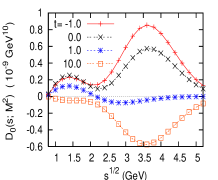
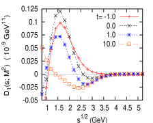
Figure 1: (Color online) The $t$-dependence of the behavior of $D_{i}(s;M^{2})$ as a function of $\sqrt{s}$. The left panel is shown for the even part ($i=0$) at $M^{2}=2.5$ GeV² and the right for the odd part ($i=1$) at $M^{2}=1.2$ GeV².

The left panel for the even part shows that the integrand with $t=1$ is successfully suppressed at $\sqrt{s}\gtrsim 2$ GeV, while in the other cases there are large contributions at $\sqrt{s}\sim 3$ GeV. On the other hand, in the odd part, the best continuum suppression takes place at $\sqrt{s}\gtrsim 3$ GeV for $t=-1$. However, the contributions in the intermediate energies ($\sqrt{s}=2\sim 3$ GeV) are still so large that the isolation of the pole contribution is inadequate. Similar tendency is also seen for $t=0,1$ except $t=10$, where we can no longer ensure the pole dominance at moderate energy. Instead, we will take an optimal $t$ giving good OPE convergence. This allows us to use lower Borel masses, where the Borel weight leads to larger continuum suppression.

The pole dominance can be checked also in Fig. 2, where we plot $C_{i}(M^{2};s_{th})$ as functions of the Borel mass with a fixed $s_{th}$. The function $C_{i}$ defined in Eq. (19) measures the pole dominance and is used for the criterion of the Borel window that the upper boundary is determined so that $C_{i}\geq 0.5$. In the left panel we plot $C_{0}$ (even part) in the case of $t=-1.0,\ 0.0,\ 0.9,\ 10.0$ with $s_{th}$ fixed to $2.2$ GeV, and in the right panel we plot $C_{1}$ (odd part) in the case of $t=-1.0,\ 0.0,\ 1.1,\ 10.0$ with $s_{th}$ fixed to $2.1$ GeV. We find that, in the even part $C_{0}$ with $t=0.9$ and in the odd part $C_{0}$ with $t=0.0$, $1.1$, the pole contribution dominates the correlation function over the wide range of the Borel mass. The appearance of cusp structures in $C_{0}$ over the range of $M^{2}=2.5\sim 3.0$ GeV² at $t=0.9$, arises as the result of large cancellation of the continuum contribution in the denominator of $C_{i}$.

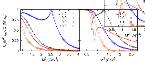
Figure 2: (Color online) The behavior of $C_{i}(M^{2};s_{th})$ as a function of $M^{2}$. The left panel is shown for the even part with $t=-1.0,0.0,0.9,10.0$ at $\sqrt{s_{th}}=2.2$ GeV and the right for the odd part with $t=-1.0,0.0,1.1,10.0$ at $\sqrt{s_{th}}=2.1$ GeV.

IV.3 The OPE convergence

Next we discuss the OPE convergence, which determines the lower boundary of the Borel windows. Shown in Fig. 3 are the ratios of highest-dimensional terms (dimension 14 in the OPE for the even part and dimension 15 for the odd one) to the whole OPE as a function of $t$ for various $M^{2}$. Here we take the Borel mass $M^{2}$ to be $2.5,2.8,3.1$ GeV² (even) and $0.7,1.0,1.3$ GeV² (odd), which are around the Borel windows set below. Our condition on the OPE convergence is that the ratios are less than 10%. For the even part having good continuum suppression at $t=1$, we consider the vicinity of $t=1$.

Figure 3: (Color online) The behavior of highest-dimensional terms of the OPE divided by the whole OPE as a function of $t$ for various $M^{2}$. The left panel is shown for the even part with $M^{2}=2.5,\ 2.8,\ 3.1$ GeV² and the right for the odd part with $M^{2}=0.7,\ 1.0,\ 1.3$ GeV².

In Fig. 3 we find quite good OPE convergence in the whole region except $t\simeq 0.95$. This remarkable convergence should be compared with the OPE of the current given in Ref. SDO , in which the convergence is not sufficient khj . The exceptionally bad convergence at $t\simeq 0.95$ is due to cancellation in the whole OPE, which is rejected by our criterion for the Borel window. If it were not the case, we would need to take account of higher-dimensional terms truncated here. In the odd part, we investigate the OPE convergence in relatively low $M^{2}$-region retaining the continuum suppression due to the Borel weight. The right panel of Fig. 3 shows that the OPE convergence is good around $t=1$, while bad around $t=-1$ where the continuum suppression is realized at higher $\sqrt{s}$. Hence we take the mixing angle around $t=1$ in the odd part as well as in the even part.

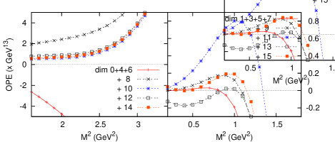
Figure 4: (Color online) OPE contributions added up each term in sequence. The left panel is shown as a function of $M^{2}$ with $t=0.9$ fixed for the even part and the right with $t=1.1$ fixed for the odd part.

To complement the issue of the OPE convergence, we illustrate OPE contributions as a function of $M^{2}$ with fixed $t$ in Fig. 4, where each dimension term is added up in sequence. We use $t=0.9$ for the even part (left panel) and $t=1.1$ for the odd part (right panel). It turns out that higher-dimensional terms become smaller for both parts.

IV.4 The Borel stability on the physical quantities

After establishing the pole dominance and the OPE convergence, we move on setting the Borel window and discussing the Borel stability on the physical quantities, i.e. mass and residue.

Fine-tuning $t$ around $t=1$ to obtain the widest Borel windows, we find our best Borel windows as $2.5\leq M^{2}\leq(2.9\sim 3.0)$ GeV² at $\sqrt{s_{th}}=2.1\sim 2.3$ GeV for the even part ($t=0.9$), and $0.7\leq M^{2}\leq(1.2\sim 1.3)$ GeV² at $\sqrt{s_{th}}=2.0\sim 2.2$ GeV for the odd part ($t=1.1$) as seen from Fig. 2. Here we have chosen the threshold parameters $\sqrt{s_{th}}$ so as to maximize the correlation with the pole at $\sqrt{s}\lesssim 2$ GeV as roughly seen in Fig. 1. These thresholds indeed give better Borel stability for the physical parameters.

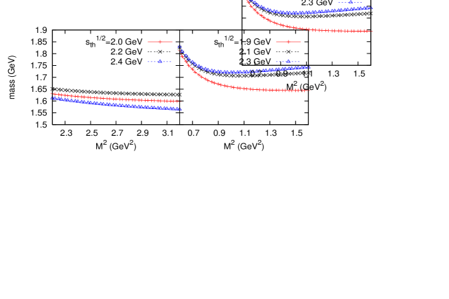
Figure 5: (Color online) The $M^{2}$-dependence of the $\Theta^{+}$ mass for the even part (left) and for the odd part (right).

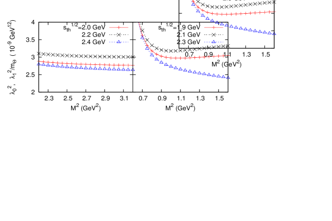
Figure 6: (Color online) The $M^{2}$-dependence of the residues ($\lambda_{0}^{2}$: left panel and $\lambda_{1}^{2}/m_{\Theta}$: right panel) in the same way with Fig. 5. Note that the residue of the odd part is divided by $m_{\Theta^{+}}$.

The values of the mass and the residue are evaluated within the Borel windows determined above. We plot the Borel mass dependence of the mass and the residue in Figs. 5 and 6, respectively, where the left (right) panel is the plot for the chiral even (odd) sum rule. Figure 5 shows that the Borel stability is established quite well within the Borel windows. The best stability is achieved with $\sqrt{s_{th}}=2.2$ GeV (even) and $2.1$ GeV (odd), giving $m_{\Theta^{+}}=1.64$ GeV (even) and $1.72$ GeV (odd) respectively. These masses slightly depend on the change of the thresholds in the range of $2.0\sim 2.4$ GeV (even) and $1.9\sim 2.3$ GeV (odd). With these uncertainties, the masses are evaluated as $m_{\Theta^{+}}=1.64\pm 0.03$ GeV (even) and $1.72\pm 0.05$ GeV (odd). The residue is evaluated in the same way as the mass from the Borel curve shown in Fig. 6. We find quite good stability again. The values of the residue are obtained from the chiral even and odd sum rules as $\lambda_{0}^{2}=(3.0\pm 0.1)\times 10^{-9}$ GeV¹² and $\lambda_{1}^{2}/m_{\Theta^{+}}=(3.4\pm 0.2)\times 10^{-9}$ GeV¹² respectively. It is remarkable that these numbers are quite similar with the close $t$. This implies that our analysis investigates consistently the same state in the two independent sum rules. Note that from the relative sign of the residue, we assign positive parity to the observed $\Theta^{+}$ state.

We investigate the dependence of the QCD parameters on our final results. We find that the final results are insensitive to the change of $m_{s}$, $R_{s}$, $m_{1}^{2}$, $\langle\bar{q}q\rangle$ and $\alpha_{s}$, and are marginally sensitive to that of $m_{0}^{2}$ and $\langle(\alpha_{s}/\pi)\,G^{2}\rangle$. By accounting for uncertainties of these QCD parameters and errors arising from our approximation, we estimate the theoretical errors of our results to be totally around 15%. Combining both results of the even and odd sum rules with this error, we finally conclude that our estimation of the $\Theta^{+}$ mass is $m_{\Theta^{+}}=1.68\pm 0.22$ GeV.

We finally confirm the OPE convergence in the mass. In Fig. 7, we plot the response of the $\Theta^{+}$ mass to addition of the higher-order OPE contributions as a function of $M^{2}$ with $t=0.9,\sqrt{s_{th}}=2.2$ GeV for the odd part (left panel) and $t=1.1,\sqrt{s_{th}}=2.1$ GeV for the odd part (right panel). We find that inclusion of higher OPE terms makes Borel curves more stable in both cases.

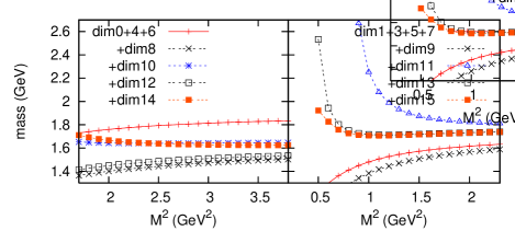
Figure 7: (Color online) The response of the $\Theta^{+}$ mass to OPE contributions as a function of $M^{2}$, where each OPE term is added up as in Fig. 4. The left panel is shown for the even part with $t=0.9,\sqrt{s_{th}}=2.2$ GeV fixed and the right for the odd part with $t=1.1,\sqrt{s_{th}}=2.1$ GeV fixed.

V Discussion

Although we have not explicitly taken into account the $KN$ scattering state appearing at about 100 MeV below the observed pentaquark mass, in this section we make a brief comment on the contamination from this scattering state. Efforts to isolate the considering $\Theta^{+}$ state from the scattering state in the analysis were recently made in su for the QSR, and in lattice for the lattice QCD. Here we explain another aspect of such isolation in more intuitive and qualitative way. The pole information of the $\Theta^{+}$ should be carried by higher-dimensional OPE terms beyond the suppressed lower-dimensional terms which have more information about the perturbative region. The property of the $\Theta^{+}$ in the QSR can be sensitive to the values of the chiral condensate $\langle\bar{q}q\rangle$, because the higher-dimensional contribution is mainly controlled by the products of the chiral condensate $\langle\bar{q}q\rangle$. Our observed states for both even and odd parts, however, are rather insensitive for the change of the order parameter, while the $KN$ threshold is expected to be sensitive, since the nucleon mass is described as the Ioffe’s formula $M_{N}\propto(-\langle\bar{q}q\rangle)^{1/3}$ in the QSR reinders . Therefore, we speculate the possible isolation of the observed states from the $KN$ scattering state. This would be also challenging for further investigating the mass shift of the $\Theta^{+}$ for chiral restoration in matter navarra in comparison with the $KN$ scattering state.

Concerning the existence of the pentaquark state, although the pronounced peak of the pentaquark has not been seen in experiments as typified by recent measurements at Jlab clas , it does not directly mean that our QSR calculations are incorrect. We faithfully follow the original idea of QSR, especially emphasizing the importance of the pole dominance and the Borel stability, then we find a pentaquark state in our analysis. When comparing such a theoretical finding to the experimental observations, one needs further steps, for instance, consideration of the reaction mechanism. The QSR just analyses spectral functions composed of resonance poles and scattering states with interpolating fields prepared appropriately. It may be the case that the ratio of the strengths between the pentaquark pole and the scattering states is different from those observed in the experiments. Our sum rule extracts successfully the pentaquark’s pole contribution from the background scattering states, such as the $KN$ state, as well as the high-energy continuum contributions. This may indicate that the low-energy scattering states are also suppressed in our linear combination of the correlation functions.

VI Summary

In this work, we have presented a new idea to address exotic hadrons with a number of quarks, such as the pentaquark, in the QSR, where the favorable continuum suppression is realized by considering a linear combination of two correlators with different chirality. Implementing the Borel technique, we indeed obtained the wide Borel windows that enable to extract hadronic properties much reliably from this analysis. We should bear in mind that as far as one relies on the simple step-function form of continuum contribution and the duality ansatz, one could not easily construct any reliable BSR’s without considering such continuum suppression. With paying attention also to the OPE convergence, we finally estimate $m_{\Theta^{+}}=1.68\pm 0.22$ GeV including uncertainties of the condensates in the OPE calculation up to dimension 15. Here the Borel curves look fairly flat and almost independent of the continuum thresholds, and such a feature is also seen for the pole residue.

We would like to point out that choice of the interpolating fields solely cannot achieve enough suppression of the large continuum contributions, since the logarithmic terms of OPE give large continuum contributions to the spectral function via the duality ansatz due to the high-dimensional current of pentaquark. To obtain sufficient continuum suppression, it is important to take a favorable linear combination of the correlation functions with the aid of chirality of the interpolating fields. This idea would be also applicable for all the correlation function analyses as in lattice QCD, where a contamination from the high-energy contributions hinders extraction of information on low-energy hadron states, and for other exotic hadrons like a tetraquark Chen:2006hy . Also, it is noteworthy that a concept of chiral symmetry introduced here plays an important role to pick up the information in the low-energy region.

- (1) LEPS Collaboration, T. Nakano et al., Phys. Rev. Lett. 91, 012002 (2003); CLAS Collaboration, S. Stepanyan et al., Phys. Rev. Lett. 91, 252001 (2003); SAPHIR Collaboration, J. Barth et al., Phys. Lett. B 572, 127 (2003); DIANA Collaboration, V. V. Barmin et al., Phys. Atom. Nucl. 66, 1715 (2003).
- (2) The first LEPS experiment was motivated by D. Diakonov, V. Petrov and M. Polyakov, Z. Phys. A 359, 305 (1997); M. Karliner and H.J. Lipkin, Phys. Lett. B 575, 249 (2003); A.W. Thomas, K. Hicks and A. Hosaka, Prog. Theor. Phys. 111, 291 (2004); See also as a review, M. Oka, Prog. Theor. Phys. 112, 1 (2004).
- (3) R.L. Jaffe and F. Wilczek, Phys. Rev. Lett. 91, 232003 (2003).
- (4) For a review of these experiments, see K. Hicks, Prog. Part. Nucl. Phys. 55, 647 (2005).
- (5) T. Nakano, talk presented at the Int. Conf. QCD and Hadronic Physics, Beijing (2005).
- (6) R. De Vita, talk presented at the APS April Meeting, Tampa (2005); CLAS Collaboration, M. Battaglieri et al., hep-ex/0510061 (2005).
- (7) J. Z. Bai et al. [BES Collaboration], Phys. Rev. D 70, 012004 (2004); I. Abt et al. [HERA-B Collaboration], Phys. Rev. Lett. 93, 212003 (2004).
- (8) M.A. Shifman, A.I. Vainshtein and V.I. Zakaharov, Nucl. Phys. B 147, 385 (1979).
- (9) B.L. Ioffe, Nucl. Phys. B 198, 175 (1981).
- (10) D. Jido, N. Kodama and M. Oka, Phys. Rev. D 54 4532 (1996).
- (11) J. Sugiyama, T. Doi and M. Oka, Phys. Lett. B 581, 167 (2004).
- (12) S.-L. Zhu, Phys. Rev. Lett. 91, 232002 (2003); R.D. Matheus et al., Phys. Lett. B 578, 323 (2004); M. Eidemüller, Phys. Lett. B 597, 314 (2004); B.L. Ioffe and A.G. Oganesian, JETP Lett. B 80, 386 (2004); T. Nishikawa, Y. Kanada-En’yo, O. Morimatsu and Y. Kondo, Phys. Rev. D 71, 076004 (2005); H.-J. Lee, N.I. Kochelev and V. Vento, hep-ph/0506250.
- (13) A.G. Oganesian, hep-ph/0510327.
- (14) R.D. Matheus and S. Narison, hep-ph/0412063.
- (15) L.J. Reinders, H. Rubinstein and S. Yazaki, Phys. Rep. 127, 1(1985).
- (16) S. Weinberg, Phys. Rev. Lett. 18, 507 (1967).
- (17) S. Sasaki, Phys. Rev. Lett. 93, 152001 (2004). In this paper, a combination of the same diquark operators with ours were first suggested as a candidate describing a pentaquark, but its detailed numerical culculations in lattice QCD have not been performed there.
- (18) Y. Chung, H.G. Dosch, M. Kremer and D. Schall, Nucl. Phys. B 197, 55 (1982).
- (19) B.L. Ioffe, Z. Phys. C 18, 67 (1983).
- (20) Y. Chung, H.G. Dosch, M. Kremer, and D. Schall, Z. Phys. C 25, 151 (1984).
- (21) T. Kojo, A. Hayashigaki and D. Jido, in preparation.
- (22) S.H. Lee, H. Kim and Y. Kwon, Phys. Lett. B 609 252 (2005); Y. Kwon, A. Hosaka and S.H. Lee, hep-ph/0505040.
- (23) T.T. Takahashi et al., Phys. Rev. D 71, 114509 (2005); N. Ishii et al., Phys. Rev. D 71, 034001 (2005); F. Csikor et al., hep-lat/0503012; O. Jahn, J.W. Negele and D. Sigaev, hep-lat/0509102; N. Mathur et al., Phys. Rev. D 70, 074508 (2004); K. F. Liu and N. Mathur, Int. J. Mod. Phys. A 21, 851 (2006).
- (24) F.S. Navarra, N. Nielsen and K. Tsushima, Phys. Lett. B 606, 335 (2005).
- (25) H. X. Chen, A. Hosaka and S. L. Zhu, hep-ph/0604049.