Phase transitions in the early and present Universe.

Abstract

The evolution of the Universe is the ultimate laboratory to study fundamental physics across energy scales that span about 25 orders of magnitude: from the grand unification scale through particle and nuclear physics scales down to the scale of atomic physics. The standard models of cosmology and particle physics provide the basic understanding of the early and present Universe and predict a series of phase transitions that occurred in succession during the expansion and cooling history of the Universe. We survey these phase transitions, highlighting the equilibrium and non-equilibrium effects as well as their observational and cosmological consequences. We discuss the current theoretical and experimental programs to study phase transitions in QCD and nuclear matter in accelerators along with the new results on novel states of matter as well as on multifragmentation in nuclear matter. A critical assessment of similarities and differences between the conditions in the early universe and those in ultrarelativistic heavy ion collisions is presented. Cosmological observations and accelerator experiments are converging towards an unprecedented understanding of the early and present Universe.

I Introduction

The current knowledge of the early and present Universe is summarized by the standard models of cosmology and of particle physics. Their symbiosis provides an unprecedented understanding of the evolution of the Universe solidly based on a wealth of observations and experiments. Particle and nuclear physics in a field theory context provide the fundamental building blocks which when combined with general relativity and statistical mechanics yield a description from the early inflationary stage through a detailed thermal history of the Universe, to the formation of large scale structure, galaxies and stars. During the last decade a large body of observational data has provided a strong evidence in support of theoretical ideas of an early stage of inflation, during which the visible size of the Universe grows exponentially. After this brief, but explosive period of inflation followed by deccelerated expansion and cooling, the Universe succesively visits the different energy scales at which particle and nuclear physics predict symmetry breaking phase transitions. The goals of this article are to review the equilibrium and non-equilibrium aspects of these phase transitions, their cosmological imprints and the current theoretical and experimental efforts to study them with accelerator experiments. The article begins with an account of both standard models, setting the stage for a discussion of phase transitions in particle and nuclear physics. A brief self-contained excursion of cosmology beginning from inflation follows the early history of the Universe, visiting the time-marks at which particle physics predicts phase transitions and exploring their potential consequences. The last phase transition(s) of the standard model of particle physics took place when the Universe was about $10^{-5}$ secs. old, they are the deconfinement-confinement and chiral phase transitions predicted by Quantum Chromodynamics (QCD). The article presents a summary of the theoretical efforts and the experimental programs in several accelerator facilities to study the QCD phase transitions as well as static and dynamical aspects of phase transitions in cold nuclear matter.

II The standard models:

The modern understanding of the early and present Universe hinges upon two standard models: the standard model of cosmology and the standard model of particle physicsbookkolb -kamion . Both have passed stringent observational and experimental tests. A wealth of cosmological data is providing confirmation of theoretical ideas in early Universe cosmology. Measurements of the temperature anisotropy of the Cosmic Microwave Background radiation (CMB) by satellite, balloon borne and earth based observations, large scale structure surveys, Lyman $\alpha$ forest, cluster abundance, weak lensing and measurements of the cosmological expansion and its acceleration by Type Ia supernovae searches, combined with high precision measurements of light element abundances provide an impressive body of high quality data that yield an unprecedented understanding of cosmology.

II.1 Observational ingredients

The main observational pillars that support the standard model of cosmology arebookkolb -kamion :

• Homogeneity and isotropy: on scales larger than $\geq 100\,\textrm{Mpc}$ the Universe looks homogeneous and isotropic. This is confirmed by large scale surveys and by the almost isotropy of the CMB.

• The Hubble expansion: objects that are separated by a comoving distance $d$ recede from each other with a velocity $v=H\,d$, with $H$ the Hubble parameter, whose value today is $H_{0}\approx 72\,\textrm{km}/s/\textrm{Mpc}$. The Hubble expansion law determines the size of our causal horizon: objects separated by a comoving distance

  $$d_{H}=3000\,h^{-1}\,\textrm{Mpc}\quad,\quad h=H_{0}/100\,\textrm{km}/s/\textrm{Mpc}$$ (1)

  recede from each other at the speed of light and are therefore causally disconnected.

• The Cosmic Microwave Background radiation (CMB): a bath of thermal photons with an almost perfect Planck distribution at a temperature $T_{0}=2.725\pm 0.001\,K$. Temperature anisotropies $\Delta T/T_{0}\sim 10^{-5}$ were first measured in 1992 by the COBE satelliteCOBE , their detection represents a triumph for cosmology. This small temperature anisotropy, whose existence is predicted by cosmological models, provide the clue to the origin of structure. It is an important confirmation of theories of the early Universe.

• The abundance of light elements: observations of the abundance of elements in low metallicity regions reveals that about $76\%$ of ordinary matter is in the form of hydrogen, about $24\%$ (by mass) in ${}^{4}He$ and trace abundances of ${}^{3}He\,(\sim 10^{-5})$, deuterium ($\sim 10^{-5}$) and ${}^{7}Li\,(\sim 10^{-10}$), all relative to hydrogensteigman ; turnerBBN . These elements were formed during the first three minutes of the Universe, while heavier elements (metals) are produced in the interior of stars and in astrophysical processes during supernovae explosions.

• The concordance model: dark matter and dark energy. In the last few years there has been a wealth of observational evidence from CMB, large scale structure and high redshift supernovae IaSN1 data that leads to the remarkable conclusions that i) the spatial geometry of the Universe is flat, ii) the Universe is accelerating today, and iii) most of the matter is in the form of dark matter. Current understanding of cosmology is based on the concordance or $\Lambda CDM$ model in which the total energy density of the Universe has as main ingredients: $5\%$ of baryonic matter, $25\%$ of dark matter and $70\%$ of dark energyWMAP1 ; kogut ; spergel ; peiris . The present observations indicate that the dark energy can be described by a cosmological constantnegra .

II.2 The building blocks

The main building blocks for a theory of the standard cosmology are:

• Gravity: Classical general relativity provides a good description of the geometry of space time for scales $l\gg l_{Pl}\sim 10^{-33}\mbox{cm}$ or time scales $t\gg t_{Pl}\sim 10^{-43}\mbox{s}$, or equivalently energy scales well below the Planck scale $M_{Pl}\sim 10^{19}\mbox{Gev}$. A consistent quantum theory of gravity unified with matter describing the physics at the Planck scale is yet to emerge.

  Homogeneity and isotropy for a spatially flat space-time lead to the Friedmann-Robertson-Walker (FRW) metric

  $$ds^{2}=dt^{2}-a^{2}(t)\;d\vec{x}^{2}$$ (2)

  where $t$ is the comoving time (the proper time of a comoving observer). Physical scales are stretched by the scale factor $a(t)$ with respect to the comoving scales

  $$l_{phys}(t)=a(t)\;l_{com}\;.$$ (3)

  A physical wavelength redshifts proportional to the scale factor [eq.(3)], therefore its time derivative obeys the Hubble law $\dot{l}_{phys}(t)=H(t)\;l_{phys}(t)=l_{phys}(t)/d_{H}(t)$. At equilibrium temperature decreases as the universe expands as

  $$T(t)=\frac{T_{0}}{a(t)}$$ (4)

  In the homogeneous and isotropic FRW universe described by eq.(2), the matter distribution must be homogeneous and isotropic, with an energy momentum tensor with the fluid form

  $$\langle T^{\mu}_{\nu}\rangle={\rm diag}[\rho,-p,-p,-p]\;,$$ (5)

  where $\rho,\;p$ are the energy density and pressure, respectively. In such geometry the Einstein equations of general relativity reduce to the Friedmann equation, which determines the evolution of the scale factor from the energy density

  $$\left[\frac{\dot{a}(t)}{a(t)}\right]^{2}\equiv H^{2}(t)=\frac{\rho}{3M^{2}_{Pl}}\,.$$ (6)

  where $M_{Pl}=1/\sqrt{8\pi G}=2.4\times 10^{18}$ GeV $=0.434\times 10^{-5}$ g. A spatially flat Universe has the critical density

  $$\rho_{c}=3\;M^{2}_{Pl}\;H^{2}_{0}=1.88\;h^{2}\;10^{-29}\textrm{g}/\textrm{cm}^{3}\,.$$ (7)

  where $H_{0}$ is the Hubble constant today. The energy momentum tensor conservation reduces to the single conservation equation,

  $$\dot{\rho}+3\left(\rho+p\right)\frac{\dot{a}}{a}=0$$ (8)

  The two equations (6) and (8) can be combined to yield the acceleration of the scale factor,

  $$\frac{\ddot{a}}{a}=-\frac{1}{6\;M^{2}_{Pl}}(\rho+3\;p)$$ (9)

  which will prove useful later. In order to provide a close set of equations we must append an equation of state $p=p(\rho)$ which is typically written in the form

  $$p=w(\rho)\;\rho$$ (10)

  The following are important cosmological solutions:

  $${\rm Cosmological~{}Constant}\;\Rightarrow w=-1:{\rm de~{}Sitter~{}expansion}\Rightarrow\rho={\rm constant}~{};~{}a(t)\propto e^{Ht}~{};~{}H=\sqrt{\frac{\rho}{3M^{2}_{Pl}}}$$ (11)

  (12)

  $${\rm Radiation}\;\Rightarrow w=\frac{1}{3}:{\rm Radiation~{}domination}\Rightarrow\rho\propto a^{-4}~{};~{}a(t)\propto t^{\frac{1}{2}}$$ (13)

  $${\rm Non-relativistic(cold)~{}Matter}\;\Rightarrow w=0:{\rm Matter~{}domination}\Rightarrow\rho\propto a^{-3}~{};~{}a(t)\propto t^{\frac{2}{3}}$$

  Furthermore, we see from eqs.(9) and (13) that accelerated expansion takes place if $w<-1/3$.

• The Standard Model of Particle Physics:SM the current standard model of particle physics, experimentally tested with remarkable precision describes the theory of strong (QCD), weak and electromagnetic interactions (EW) as a gauge theory based on the group $SU(3)_{c}\otimes SU(2)\otimes U(1)_{Y}$. The particle content is: three generations of quarks and leptons:

  $$\left(\begin{array}[]{c}u\\ d\end{array}\right)\left(\begin{array}[]{c}c\\ s\end{array}\right)\left(\begin{array}[]{c}t\\ b\end{array}\right)\;;\;\left(\begin{array}[]{c}\nu_{e}\\ e\end{array}\right)\left(\begin{array}[]{c}\nu_{\mu}\\ \mu\end{array}\right)\left(\begin{array}[]{c}\nu_{\tau}\\ \tau\end{array}\right)$$

  vector Bosons: 8 gluons (massless) , $Z^{0}$, $W^{\pm}$ with masses $M_{Z}=91.18\pm 0.02$ GeV and $M_{W}=80.4\pm 0.06$ GeV, the photon (massless) and the scalar Higgs, although the experimental evidence for the Higgs bosons is still inconclusive.

Current theoretical ideas supported by the renormalization group running of the couplings propose that the strong, weak and electromagnetic interactions are unified in a grand unified theory (GUT) at the scale $M_{GUT}\sim 10^{16}$ Gev. Furthermore the ultimate scale at which Gravity is eventually unified with the rest of particle physics is the Planck scale $M_{Pl}\sim 10^{19}\mbox{Gev}$. Although there are proposals for the total unification of forces within the context of string theories, their theoretical understanding as well as any experimental confirmation is still lacking. However, the physics of the standard model of the strong and electroweak interactions that describes phenomena at energy scales below $\sim 100$ GeV is on solid experimental footing.

The connection between the standard model of particle physics and early Universe cosmology is through Einstein’s equations that couple the space-time geometry to the matter-energy content. As argued above, gravity can be studied semi-classically at energy scales well below the Planck scale. The standard model of particle physics is a quantum field theory, thus the space-time is classical but with sources that are quantum fields. Semiclassical gravity is defined by the Einstein’s equations with the expectation value of the energy-momentum tensor $\hat{T}^{\mu\nu}$ as sources

$$G^{\mu\nu}=R^{\mu\nu}-\frac{1}{2}\,g^{\mu\nu}R=\frac{\langle\hat{T}^{\mu\nu}\rangle}{M^{2}_{Pl}}\;.$$ (14)

The expectation value of $\hat{T}^{\mu\nu}$ is taken in a given quantum state (or density matrix) compatible with homogeneity and isotropy which must be translational and rotational invariant. Such state yields an expectation value of the energy momentum tensor with the fluid form eq.(5).

Through this identification the standard model of particle physics provides the sources for Einstein’s equations. All of the elements are now in place to understand the evolution of the early Universe from the fundamental standard model. Einstein’s equations determine the evolution of the scale factor, the standard model provides the energy momentum tensor and statistical mechanics provides the fundamental framework to describe the thermodynamics from the microscopic quantum field theory of the strong, electromagnetic and weak interactions.

II.3 Energy scales, time scales and phase transitions

Energy Scales:

While a detailed description of early Universe cosmology is available in several books bookkolb -liddlerev , a broad- brush picture of the main cosmological epochs can be obtained by focusing on the energy scales of particle, nuclear and atomic physics.

• Total Unification: Gravitational, strong and electroweak interactions are conjectured to become unified and described by a single quantum theory at the Planck scale $\sim 10^{19}$ Gev. There are currently many proposals that seek to provide such fundamental description such as string theories, however, their theoretical consistency is still being studied and experimental confirmation is not yet available.

• Grand Unification: Strong and electroweak interactions (perhaps with supersymmetry) are expected to become unified at an energy scale $\sim 10^{16}$ Gev corresponding to a temperature $T\sim 10^{29}$ K under a larger gauge group $G$, for example $SU(5),\;SO(10),\;E_{8}$, which breaks spontaneously $G\rightarrow SU(3)_{c}\otimes SU(2)\otimes U(1)_{Y}$ at a scale below grand unification. There are very compelling theoretical reasons for the existence of the GUT scale such as the merging of the running coupling constants of the strong, electromagnetic and weak interactions, shown in fig. 1 for the minimal supersymmetric standard model (MSSM). Yet another reason is the explanation of the small neutrino masses via the see-saw mechanism in terms of the ratio between the weak and the grand unification scale.

  

  Figure 1: Evolution of the weak $\alpha_{1}$, electromagnetic $\alpha_{2}$ and strong $\alpha_{3}$ couplings with energy in the MSSM model. Notice that only $\alpha_{3}$ decreases with energy (asymptotic freedom) extracted from ref.unifica

• Electroweak : Weak and electromagnetic interactions become unified in the electroweak theory based on the gauge group $SU(2)\otimes U(1)_{Y}$. The weak interactions become short ranged after a symmetry breaking phase transition $SU(2)\otimes U(1)_{Y}\rightarrow U(1)_{em}$ at an energy scale of the order of the masses of the $Z^{0},W^{\pm}$ vector bosons, corresponding to a temperature $T_{EW}\sim 100$ GeV $\sim 10^{15}$ K. At temperatures $T>T_{EW}$ the symmetry is restored and all vector bosons are (almost) massless (but for plasma effects that induce screening masses). For $T<T_{EW}$ the vector bosons that mediate the weak interactions (neutral and charged currents) $W^{\pm},Z^{0}$ acquire masses through the Higgs mechanism while the photon remains massless, corresponding to the unbroken $U(1)$ abelian symmetry of the electromagnetic interactions. Thus $T_{EW}$ determines the temperature scale of the electroweak phase transition in the early Universe and is the earliest phase transition that is predicted by the standard model of particle physics. The understanding of the symmetry breaking sector of the standard model is one of the primary goals of the Large Hadron Collider at CERN. The standard model has the necessary ingredients to explain the origin of the baryon asymmetry, leading to the possibility that the asymmetry between matter and antimatter was produced at the electroweak scale (see section V).

• QCD: The strong interactions have a typical energy scale $\Lambda_{QCD}\sim\,200$ MeV at which the coupling constant becomes strong [$\alpha_{s}\sim\mathcal{O}(1)$]. This energy scale corresponds to a temperature scale $T_{QCD}\sim 10^{12}$K. QCD is an asymptotically free theory, the coupling between quarks and gluons becomes smaller at large energies, but it diverges at the scale $\Lambda_{QCD}$. For energy scales below $\Lambda_{QCD}$ QCD is a strongly interacting theory and quarks and gluons are bound into mesons and baryons. This phenomenon is interpreted in terms of a phase transition at an energy scale $\Lambda_{QCD}$ or $T_{QCD}$. For $T>T_{QCD}$ the relevant degrees of freedom are weakly interacting quarks and gluons, while below are hadrons. This is the quark-hadron or deconfinement-confinement phase transition. In the limit of massless up and down quarks, QCD features an $SU(2)_{L}\otimes SU(2)_{R}$ chiral symmetry, which is spontaneously broken at about the same temperature scale as the confinement-deconfiment transition. Pions are the (quasi) Goldstone bosons emerging from the breakdown of the chiral symmetry $SU(2)_{L}\otimes SU(2)_{R}\rightarrow SU(2)_{R+L}$. The QCD phase transition(s) are the last phase transition predicted by the standard model of particle physics. The high temperature phase above $T_{QCD}$, with almost free quarks and gluons (because the coupling is small by asymptotic freedom) is a quark-gluon plasma or QGP. Experimental programs at CERN (SPS-LHC) and BNL (AGS-RHIC) study the QCD phase transition via ultrarelativistic heavy ion collisions (URHIC) and a systematic analysis of the data gathered at SPS and RHIC during the last decade has given an optimistic perspective of the existence of the QGPphystoday ; heinz (see section 4 below).

• Nuclear Physics: Low energy scales that are relevant for cosmology are determined by the binding energy of light elements, in particular deuterium, whose binding energy is $\sim 2$ Mev corresponding to a temperature $T\sim 10^{10}$ K. This is the energy scale that determines the onset of primordial nucleosynthesis. The first step in the network of nuclear reactions that yield the primordial elements is the formation of the deuteron via $n+p\leftrightarrow d+\gamma$. The large number of photons per baryon results in that high energy photons in the blackbody tail dissociate the deuterons formed in the forward reaction until the temperature becomes of the order of $T_{NS}\sim 0.1\,\textrm{MeV}$. Once deuterons are formed, a network of nuclear reactions results in that all neutrons end up in nuclei, mainly helium, resulting in a helium abundance of about $25\%$steigman ; turnerBBN . The nature of the nuclear forces suggests the possibility of a liquid-gas phase transition in cold nuclear matter at an energy $\sim 15-20\,\textrm{MeV}$ discussed in section VIII.5.

• Atomic Physics: A further very important low energy scale relevant for cosmology corresponds to the binding energy of hydrogen $\sim 10~{}\textrm{eV}$. This is the energy scale at which free protons and electrons combine into neutral hydrogen or ‘recombination’. The large number of photons per baryon results in that recombination actually takes place at an energy scale of order $0.3~{}\textrm{eV}$, at about $400000$ years after the beginning of the Universe. At this time when neutral hydrogen is formed the Universe becomes transparent. This event determines the last scattering surface, after neutral hydrogen is formed photons no longer scatter and travel freely. These are the photons measured by CMB experiments today.

Time Scales: An important ingredient of modern standard cosmology is a brief but explosive early period of inflation during which the scale factor grows exponentially as $a(t)=e^{Ht}$ [see eq. (11)]. WMAPWMAP1 ; kogut ; spergel ; peiris yields an upper bound on the energy scale of the inflation [for a detailed discussion see sec. IV.3] $H\lesssim 10^{13}$ GeV. In order to solve the entropy and horizon problems, the inflationary stage must last a time interval $\delta t$ so that $H\;\delta t\sim 60$, hence the inflationary stage lasts a time scale

$$\Delta t_{inf}\sim 10^{-34}\,\textrm{secs}\;.$$ (15)

Field models of inflation are discussed in sec. IV.3. The inflationary stage is followed by a radiation dominated era (standard hot big bang) after a short period of reheating during which the energy stored in the field that drives inflation decays into quanta of many other fields, which through scattering processes reach a state of local thermodynamic equilibrium.

Once local thermodynamic equilibrium is reached, a very detailed picture of the thermal history of the Universe emerges combining statistical mechanics with the basic ingredients described above  bookkolb -liddlerev : during the first $\sim 10000$ years of the Universe and after the inflationary stage that lasted $\sim 10^{-34}$secs, the Universe was radiation dominated expanding and cooling (almost) adiabatically. As a consequence the entropy $S\propto V(t)\;T^{3}(t)\propto V_{0}\;\left[a(t)\;T(t)\right]^{3}$ is almost constant according to eq.(4) but for the change in the number of relativistic degrees of freedom. Therefore, for a relativistic equation of state $p=\rho/3$ with $p$ being the pressure and $\rho$ the energy density, $\rho(t)\propto T^{4}(t)$. Such equation of state yields the following evolution of the scale factor as a function of time

$$H=\frac{1}{2t}=0.33\,g^{\frac{1}{2}}\frac{T^{2}}{M_{Pl}}$$ (16)

where $g$ is the number of relativistic degrees of freedom, which is also a function of temperature $10\lesssim g\lesssim 100$ for $0.5\,\textrm{MeV}\lesssim T\lesssim 300\,\textrm{GeV}$. The above expression yields a simple dictionary that allows to translate temperature (or energy scale) into time scales, namely

$$T\sim\frac{\textrm{MeV}}{\sqrt{t(\textrm{sec})}}\sim\frac{10^{10}\,\textrm{K}}{\sqrt{t(\textrm{sec})}}\;.$$ (17)

This simple dictionary allows to establish the time scales at which the standard model of particle physics predicts phase transitions as well as an estimate of whether the transitions are likely to occur in LTE or not. The electroweak transition would have ocurred at $T\sim 100\,\textrm{GeV}$ at a time scale $t_{EW}\sim 10^{-12}\,\textrm{secs}$ and the QCD phase transition at $T\sim 170\,\textrm{MeV}$ at $t_{QCD}\sim 10^{-5}\,\textrm{secs}$.

Local Thermal Equilibrium (LTE) or Nonequilibrium:

Whether a phase transition occurs in or out of local thermodynamic equilibrium (LTE) depends on the comparison of two time scales: the cooling rate and the rate of equilibration. In the early Universe or in ultrarelativistic heavy ion collisions, the rate of change of temperature is determined by the expansion rate of the fluid. The rate of cooling by cosmological expansion follows from eq.(4) $\dot{T}(t)/T(t)=-\dot{a}(t)/a(t)=-H(t)$. Collisions as well as non-collisional processes contribute to establish equilibrium with a rate $\Gamma$. Local thermodynamic equilibrium ensues when $\Gamma>H(t)$, in which case the evolution is adiabatic in the sense that the thermodynamic functions depend slowly on time through the temperature. When the cosmological expansion is too fast, namely $H(t)\gg\Gamma$, local thermodynamic equilibrium cannot ensue, the temperature drops too fast for the system to have time to relax to LTE and the phase transition occurs via a quench from the high into the low temperature phase.

While a detailed understanding of the relaxational dynamics requires an analysis via quantum Boltzmann equations, a simple order of magnitude estimate for a collisional rate is given by the ensemble average $\Gamma\sim\langle\sigma\,n\,v\rangle$, where $\sigma$ is a scattering cross section, $n$ is the density of scatterers and $v$ the average velocity. For electromagnetic scattering a typical cross section is of order $\sigma_{em}\sim\alpha^{2}/Q^{2}$ with $Q^{2}$ the transferred momentum, at high temperature single photon exchange yields the estimate $\sigma_{em}\sim\alpha^{2}/T^{2}$, the density of ultrarelativistic degrees of freedom $n\sim T^{3}$ and $v\sim 1$ yields $\Gamma_{em}\sim\alpha^{2}\;T$. In QCD, simple gluon exchange yields the estimate $\Gamma_{QCD}\sim\alpha^{2}_{s}\;T$. Comparing with $H$ given by eq.(16), it is found that the strong interactions are in LTE for $T\lesssim 10^{16}$ GeV and electromagnetic interactions are in LTE for $T\lesssim 10^{14}$ GeV. A similar estimate is obtained for the weak interactions: a typical scattering process with energy transferred $E\ll M_{W}$ has a scattering cross section $\sigma\sim G^{2}_{F}\;E^{2}$ whereas if $E>>M_{W},\;\sigma\sim g^{4}/E^{2}$, therefore in a thermal medium with $E\sim T$ and density of relativistic particles $n\sim T^{3}$ a typical weak interaction reaction rate is $\Gamma_{EW}\sim g^{4}\;T$ for $T\gg M_{W,Z}$, and $\Gamma_{EW}\sim G^{2}_{F}\;T^{5}$ for $T\ll M_{W,Z}$. In this latter temperature regime the ratio $\Gamma_{EW}/H\sim(T/\textrm{MeV})^{3}$, hence the weak interactions fall out of LTE for $T\lesssim 1$ MeV. This simple analysis, while providing an intuitive order of magnitude estimate for the relaxation time scales, neglects several subtle but important aspects that must be studied on a case-by-case basis:

• Screening and infrared phenomena: the estimate for the relaxational rates $\Gamma$ invoked the exchange of a vector boson or relativistic degrees of freedom. In a medium at high temperature and or density there are important screening effects and infrared phenomena that change these assessments both quantitatively and qualitatively and depend on whether the gauge symmetry is abelian or nottembooks .

• Critical slowing down: condensed matter experiments reveal that systems that undergo second order (or in general continuous) transitions exhibit a slowing down of relaxational dynamics of long wavelength fluctuations near the critical point of a phase transition. Such is the case in ferromagnets, superconductors and superfluids. While short wavelength fluctuations remain in LTE through the transition through microscopic scattering mechanisms, long wavelength fluctuations feature slower relaxational dynamics and even cooling rates far smaller than microscopic relaxational rates produce quenched transitions and departures from equilibrium. Critical slowing down in classical models of critical phenomena is fairly well understoodgolden ; langer ; guntonmiguel , but a similar level of understanding in quantum field theories at extreme temperature and density is now emergingboycrit .

• Strong first order transitions and metastable states: In a strong first order transition (see below) the system is trapped in a metastable state which is a local minimum of the free energy but not the global one. Within this local, metastable minimum, collisions can bring the system to LTE, but the metastable state will eventually decay and fall out of LTE by the non-perturbative process of nucleation, which is described below in detail.

II.4 Phase transitions: early Universe vs. accelerator experiments

The control variables in a collision experiment are the beam energy and the luminosity. For a phase transition to be achieved in an accelerator experiment an environment with a temperature close to the transition value $T_{c}$ must be formed in the collision region. The blackbody relation, valid for ultrarelativistic particles in equilibrium yields the energy density-temperature relation

$$\varepsilon=C\,T^{4}\;,$$ (18)

where the constant $C$ depends on the number of degrees of freedom. For the electroweak phase transition with $T_{c}\sim 100\,\textrm{GeV}$, the energy density that must be deposited in the collision region to achieve the conditions for a phase transition is $\varepsilon\sim 10^{10}\,\textrm{GeV}/\textrm{fm}^{3}$. This energy density is about $10^{11}$ times larger than that of nuclear matter. For the QCD phase transition with $T_{c}\sim 177\,\textrm{MeV},\;\varepsilon\sim\textrm{GeV}/\textrm{fm}^{3}$ which is achieved in ultrarelativistic heavy ion collisions at SPS-CERN and RHIC-BNL. Therefore, from the perspective of studying particle physics phase transitions with accelerator experiments the only realistic possibility for the foreseeable future is the QCD transition with URHIC at RHIC and the forthcoming LHC. Hence the potential observables from phase transitions in the early Universe before the QCD scale must be inferred indirectly from the aftermath. In section VIII.4 we compare the conditions for the QCD phase transition both in the early Universe and in URHIC to assess whether current experiments reproduce the conditions that prevailed about $10\,\mu\,\textrm{secs}$ after the beginning of the Universe.

III Phase Transitions: equilibrium and non-equilibrium aspects:

III.1 Equilibrium aspects: free energy, effective potentials and critical phenomena.

Phase transitions are broadly characterized as either second or first ordergolden ; langer ; guntonmiguel . In the Landau theory of phase transitions the order parameter plays a central role. In particle physics the order parameter is the expectation value of a spin zero field in the state that extremizes the free energy. A non-zero expectation value for a non-zero spin field entails the breakdown of rotational symmetry. A particularly illuminating example is that of ferromagnetic materials where the order parameter is the total magnetization of the sample. For these materials the magnetization vanishes above the Curie temperature while a nonzero spontaneous magnetization emerges below such critical temperature. In the standard model, the order parameter is the expectation value of the neutral component of the Higgs $\langle\varphi_{0}\rangle$, in QCD the chiral order parameter is the expectation value of the pseudoscalar density $\langle\bar{\psi}\gamma^{5}\psi\rangle$. For the confinement-deconfinement phase transition lattice studies show a rapid variation of the free energy as a function of temperature and the Polyakov loop may play the role of order parameter (see below).

At zero temperature and chemical potential the state of lowest free energy is the vacuum state of the theory. An important concept to study the nature of the phase transition is that of the effective potential or Gibbs free energy which is a function of the expectation value of the scalar field.

Consider adding to the Hamiltonian of the theory $H$ a term $J\,\varphi$ where $J$ is a constant and $\varphi$ is the scalar field whose expectation value is the order parameter. The total Hamiltonian is $H[J]=H+J\,\varphi$. The partition function is given by

$$Z[J,T]=\textrm{Tr}\,e^{-\frac{H[J]}{T}}\,$$ (19)

introducing the Helmholtz free energy

$$W[T,J]=-T\,\ln Z[J,T]\;,$$ (20)

the order parameter $\Phi$ is given by

$$\frac{\delta W[T,J]}{\delta J}=\Phi\;,$$ (21)

inverting this relation one finds $J(\Phi)$. The Gibbs free energy or effective potential $V[\Phi]$ follows from a Legendre transform

$$V[\Phi]=W[J(\Phi)]-J(\Phi)\,\Phi\;,$$ (22)

and it is a function of the order parameter and other intensive thermodynamic variables such as temperature, chemical potential, etc. It is a very powerful concept that provides information on the equilibrium thermodynamic aspects and the phase structure of the theory and the possible transitions between them.

Figure 2: Effective potentials for a second order phase transition with the breakdown of a discrete symmetry (left panel) and for a first order phase transition (right panel). The filled circles in the right panel figure display the equilibrium minima for $T>T_{c}$ and $T=T_{c}$ and the metastable minimum for $T<T_{c}$.

Fig. 2 displays the typical effective potentials for a second order (left panel) and first order (right panel) phase transitions. In the case of a second order transition, the order parameter in the state of minimum free energy vanishes continuously as the temperature approaches the critical. In second order phase transitions the second derivative of the free energy with respect to temperature is divergent at the critical temperature. Near the critical temperature the free energy per unit volume, or equivalently the pressure varies as $p(T)\sim|T-T_{c}|^{2-\alpha}$ with $\alpha$ the thermal critical exponent. The order parameter itself vanishes as $|T-T_{c}|^{\beta}$ for $T\rightarrow T_{c}$ from below, with $\beta>0$ and response functions feature power-law singularities. In contrast to this case, in a first order phase transition the value of the order parameter and the position of the minimum of the free energy jump discontinuously at the critical temperature. In fig. 2 the black circles in the right panel show the behavior of the order parameter as the temperature is lowered from above to below $T_{c}$. The state that minimizes the effective potential changes suddenly from the right to the left well as the temperature is lowered below $T_{c}$. For $T>T_{c}$ the right well in the right panel remains a local minimum of higher free energy, thus a metastable state. The difference in free energies between the local and the global minima yields a latent heat which is released upon the decay of the metastable state.

The effective potential also provides information on the excitation spectrum. Consider a state characterized by a given value of the order parameter $\Phi$, the frequency of harmonic excitations of wavevector $k$ around this state is given by

$$\Omega(k;\Phi)=\sqrt{k^{2}+V^{\prime\prime}(\Phi)}\,~{}~{},~{}~{}V^{\prime\prime}(\Phi)=\frac{d^{2}V(\Phi)}{d\Phi^{2}}\,.$$ (23)

Most of the phase transitions in particle physics models involve the spontaneous breakdown of a global symmetry and the order parameter transforms covariantly under this symmetry. An expectation value of the order parameter in the state of lowest free energy indicates the spontaneous breakdown of the symmetry. Different phase transitions in particle physics involve different order parameters: for the electroweak transition the order parameter is the expectation value of the Higgs doublet along the neutral component, $\Phi=\langle\varphi_{0}\rangle$. This expectation value breaks the symmetry $SU(2)\otimes U(1)_{Y}\rightarrow U(1)_{em}$, the three Goldstone bosons emerging from the global broken symmetry make up the longitudinal components of the $W^{\pm},Z^{0}$ vector bosons via the Higgs mechanism. In QCD with massless quarks the expectation value of the chiral density $\langle\bar{\Psi}\gamma^{5}\Psi\rangle$ with $\Psi$ an up-down quark doublet breaks the $SU(2)_{L}\otimes SU(2)_{R}$ symmetry of the QCD Lagrangian down to $SU(2)_{L+R}$ with pions emerging as the triplet of Goldstone bosons. Because up and down quarks are not exactly massless, pions are pseudo Goldstone bosons. The QCD confinement-deconfinement transition does not have an obvious order parameter. However, in absence of dynamical quarks, for example in an $SU(N)$ Yang-Mills theory of gluons, the Polyakov loop

$$L(x)=\frac{1}{N}\left\langle\,\textrm{Tr}\,\mathcal{P}\exp\left(ig\int_{0}^{\frac{1}{T}}\textbf{A}_{0}(\vec{x},\tau)\;d\tau\right)\right\rangle$$ (24)

has been shown to be a suitable gauge invariant order parameter. In the above expression $g$ is the gauge coupling, $T$ is the temperature $\textbf{A}_{0}$ is the temporal component of the $SU(N)$ gauge potential, and $\mathcal{P}$ is the path ordering symbol, the line integral is carried out in Euclidean time. The Polyakov loop is usually interpreted as the free energy of an infinitely heavy test quark. It vanishes in the confined phase for $T<T_{c}$ and is non-vanishing in the deconfined phase $T>T_{c}$. An effective potential in terms of the Polyakov line has recently been proposed to study the confining-deconfining phase transitionpolypisa . When light dynamical quarks are included there is no longer an obvious order parameter for the confinement-deconfinement phase transition because light dynamical quarks screen the potential from gluon exchange.

Second order phase transitions in equilibrium and critical phenomena: Consider a continuous (second order) phase transitiongolden described by an effective potential akin to the left panel in fig. 2 in the case in which the temperature falls from a value larger than the critical value $T_{c}$. If the cooling rate is much smaller than the relaxation rate the evolution will be in LTE, but as the temperature approaches the critical, collective long-wavelength fluctuations develop and become strongly correlated. Near $T_{c}$ these collective long-wavelength fluctuations become massless (critical), their correlation function becomes scale invariant and large regions behave coherently with strong correlations over arbitrarily large scales. This is the hallmark of critical phenomena at second order phase transitions which are characterized by response functions that feature singularities in $|T-T_{c}|$ in terms of power laws with critical exponents. The correlation function of the order parameter field $\Phi$ is given by $\langle\Phi(\vec{x})\Phi(\vec{0})\rangle\propto e^{-x/\xi(T)}$. The correlation length $\xi(T)$ diverges at the critical temperature as $\xi(T)\sim|T-T_{c}|^{-\nu}$, with $\nu>0$ being a critical exponent. At this point the system becomes correlated over large distances and the spectrum of long-wavelength fluctuations becomes scale invariant. This is a very important aspect of critical phenomena associated with second order phase transitions. Near the critical point where the correlation length diverges the long distance physics is universal and the static aspects can be described in terms of a Landau-Ginzburg low energy effective theory. The different universality classes that characterize the different critical exponents, are determined by few properties of the system such as the dimensionality, the symmetry of the order parameter, the number of independent fields, etc. The description of static critical phenomena in terms of the Landau-Ginzburg approach has been confirmed by a wealth of experiments in condensed matter systems. A relevant example of a Landau-Ginzburg description for the case of a scalar field, whose expectation value breaks a discrete symmetry $\varphi\rightarrow-\varphi$ is described by the finite temperature effective potential given by

$$V[\Phi;T]=\frac{a}{2}\;(T-T_{c})\;\Phi^{2}+\frac{b}{4}\;\Phi^{4}$$ (25)

and featured in fig.2. The concept of universality classes that describes critical phenomena for a wide variety of systems is of fundamental importance. Relevant to the discussion below is the case of the chiral phase transition in QCD, which for massless up and down quarks, is described by the same universality class as the Heisenberg ferromagnet with $O(4)$ symmetryraja .

An important dynamical aspect of second order phase transitions is that near the critical region the relaxation time scale of long-wavelength fluctuations feature critical slowing downlanger ; guntonmiguel ; golden . Critical slowing down has been studied theoretically and experimentally in condensed matter systems, where a large body of experimental work confirms the critical slowing down of these fluctuations near second order phase transitions in classical systems in agreement with theory. The study of critical slowing down in quantum field theory has recently began to receive attention boycrit . For any finite cooling rate, long-wavelength modes will be quenched through the phase transition. The effective potential provides only an equilibrium description but does not address the issue of the dynamics of the transitions between different phases.

III.2 Non-equilibrium aspects: spinodal decomposition and nucleation.

As discussed in sec.II.3 whether a phase transition occurs in LTE or not depends on whether, $\Gamma>H(t)$ or $\Gamma<H(t)$, respectively. In the first case the transition occurs adiabatically (similar to the Minkowski case) while in the latter case, the phase transition occurs via a quench from the high into the low temperature phase. The dynamics are different depending on whether the equilibrium effective potential describes a second or first order transition.

III.2.1 Second order case: spinodal decomposition

Let us first consider the simpler case of a symmetry breaking second order transition where the symmetry that breaks spontaneously is discrete. To focus on a simple, yet relevant example, consider the form for the finite temperature effective potential given by eq.(25). For $T>T_{c}$ the state of minimum free energy corresponds to $\Phi=0$, whereas for $T<T_{c}$ the state of minimum free energy corresponds to either the right or left equilibrium minima in fig. 2, namely $\Phi=\pm\Phi_{e}$ with $\Phi_{e}=\pm\left[\frac{aT_{c}}{b}(1-\frac{T}{T_{c}})\right]^{\frac{1}{2}}$. The inflection points at which $V^{\prime\prime}(\Phi,T)=0$ are at $\Phi=\pm\Phi_{s}$ with $\Phi_{s}=\left[\frac{aT_{c}}{3b}(1-\frac{T}{T_{c}})\right]^{\frac{1}{2}}$. The states with $-\Phi_{s}\leq\Phi\leq+\Phi_{s}$ are thermodynamically unstable. In order to understand the non-equilibrium aspects of a rapid phase transition it is convenient to plot the coexistence lines at which thermodynamic equilibrium states coexist and the spinodal line that limits the region of thermodynamic stability in the $T-\phi$ plane. These are shown in fig. 3. The coexistence line is given by the relation between $\Phi$ and $T$ for the minima of the potential, namely $T_{coex}(\Phi)=-b\;\Phi^{2}/a+T_{c}$, and similarly the spinodal line is determined by the condition $V^{\prime\prime}(\Phi,T)=0$, namely the inflexion points of the effective potential, which yields $T_{sp}(\Phi)=-b\;\Phi^{2}/(3\;a)+T_{c}$. Fig. 3 depicts a quench from a high temperature state with vanishing order parameter to a low temperature state when the equilibrium state corresponds to a broken symmetry. In classical statistical mechanics out of equilibrium the dynamics of the evolution out of equilibrium is studied via purely dissipative equations of motion, the Cahn-Hilliard equationslanger ; guntonmiguel ; golden . The initial stages of spinodal decomposition in classical systems are characterized by growth of unstable long-wavelength perturbations which lead to the formation of domains and coarseninglanger ; guntonmiguel . Beautiful experiments in phase separation and spinodal decomposition in binary fluids have provided a spectacular confirmation of this mechanism as well as the dynamical aspects predicted by the Cahn-Hilliard theorygoldburg . In quantum field theory the dynamics is determined by the unitary time evolution of an initially quantum state or density matrix. Quantum spinodal decomposition is studied in ref.calzetta ; danspino and the non-linear backreaction of unstable fluctuations was studied in danspino by implementing a non-perturbative self-consistent method. States between the spinodal lines are thermodynamically unstable to small amplitude long-wavelength perturbations, since $V^{\prime\prime}(\Phi)<0$ in the spinodal region $-\Phi_{s}\leq\Phi\leq+\Phi_{s}$, the frequency of small amplitude fluctuations around this state become imaginary for wavevectors $k<|V^{\prime\prime}(\Phi)|$, while fluctuations with $k>|V^{\prime\prime}(\Phi)|$ remain stable. Fluctuations with wavevectors in the spinodal band $k<\sqrt{|V^{\prime\prime}(0)|}$ grow as $e^{\gamma_{k}\,t}$ with $\gamma_{k}=\sqrt{|V^{\prime\prime}(0)|-k^{2}}$. These unstable modes lead to the formation of domains whose size is determined by a time dependent correlation length $\xi(t)$. Inside these domains the expectation value attains the equilibrium values $\pm\Phi_{e}$ at the final temperature. The formation of correlated domains of each phase is the hallmark of the process of phase separation via spinodal decomposition. The dynamics of this process is non-perturbative: initially long wavelength fluctuations grow exponentially until they become non-linear and react back on the dynamics shutting off the instabilities. In scalar field theories it is found that during the initial stages of phase separation $\xi(t)\propto t$.

Figure 3: A quench into the spinodal region.

The above discussion focused on the case of discrete symmetry that is spontaneously broken. When the broken symmetry is continuous a wealth of fascinating non-perturbative topological excitations emerge, such as vortices, monopoles, and texturestopo .

III.2.2 First order phase transitions: nucleation

The dynamics of first order phase transition is different: in this case the thermodynamic state of the system is a trapped metastable state, locally stable under small thermodynamic perturbations, but with a higher free energy than the global minimumlanger ; guntonmiguel . This is the situation of the liquid-gas phase transition for example in water. The metastable state is stable under small amplitude perturbations (oscillations in the right-most well in fig. 2) but decays via spontaneous large amplitude fluctuations corresponding to bubbles of the stable phase immersed in a host of the metastable state. Consider a spherical such bubble or radius $R$, where inside of the bubble the value of the order parameter is that of the globally stable state, but outside is that of the metastable state. Since the globally stable state has a lower free energy than the metastable state, there is a gain in the free energy given by $-4\pi R^{3}\Delta V/3$ where $\Delta V$ is the difference in the effective potential between the stable and the metastable state. Because the order parameter is inhomogeneous in this configuration there is an elastic contribution to the free energy from the gradients of the order parameter field which is proportional to the surface of the bubble, because this is the region in which the spatial derivatives of the order parameter are non-vanishing. This elastic contribution is positive and given by $4\pi R^{2}\,\sigma$ where $\sigma$ is the surface tension, thus the total change in the free energy for such inhomogeneous bubble configuration is

$$E[R]=4\pi R^{2}\sigma-\frac{4\pi}{3}\,R^{3}\Delta V\,.$$ (26)

This change in the free energy is depicted in fig. 4.

Figure 4: $E(R)$ vs. $R$, arbitrary units.

Bubbles with radii $R<R^{*}=2\sigma/\Delta V$ shrink while those with $R>R^{*}=2\sigma/\Delta V$ grow and convert the metastable phase into the globally stable phase releasing the latent heat. The phase transition completes via percolation of these growing bubbles. The probability of a bubble to appear spontaneously in the heat bath in equilibrium at temperature $T$ is given by

$$P(R^{*})=D\,e^{-\frac{E[R^{*}]}{T}}~{}~{};~{}~{}E[R^{*}]=\frac{16\pi}{3}\frac{\sigma^{3}}{(\Delta V)^{2}}$$ (27)

where the prefactor $D$ depends on the spectrum of small amplitude fluctuations around the critical bubble configuration. The rate of decay per unit volume and per unit time of the metastable state is given bylanger ; guntonmiguel ; golden

$$\Gamma=\Gamma_{0}\,e^{-\frac{E[R^{*}]}{T}}$$ (28)

where $\Gamma_{0}$ depends on the prefactor $D$ as well as in general on transport properties such as the heat conductivitylanger ; guntonmiguel . These processes which require large amplitude fluctuations to overcome a potential barrier, which in this case is determined by $E[R^{*}]$ are called thermally activated and the decay rate features the Boltzmann suppression factor corresponding to the energy of the configuration at the top of the barrier. Since the metastable state has a higher free energy than the globally stable state, the nucleation process that results in the conversion of the metastable into the stable phase must release the latent heat.

III.2.3 Liquid-gas phase transition: phase coexistence

Another important and very relevant example of a first order phase transition is the liquid-gas transition. This transition is exemplified by an equation of state of the Van der Walls form and results in general when the microscopic interactions have a short range repulsive and a long range attractive components. Such is the case of nuclear forces between nucleons (see section VIII.5). Fig. 5 displays a few isotherms for a typical equation of state in terms of pressure $P$ vs. density $\rho$ for a liquid-gas type transition. For $T>T_{c}$ the isotherms are single valued, there is only one value of density $\rho$ for a given pressure $P$ and the system is in one phase. However, for $T<T_{c}$, for a given value of the pressure there are three values of the density. The derivative $\partial P/\partial\rho|_{T}=c^{2}_{s,T}$, where $c_{s,T}$ is the isothermal speed of sound for hydrodynamic modes. Obviously, we see that $c^{2}_{s,T}<0$ in the region between $\rho_{a}$ and $\rho_{b}$ in fig.5. This corresponds to an imaginary speed of sound, therefore to unstable density fluctuations that grow exponentially with time as $e^{k\;|c_{s,T}|\;t}$. Therefore, such unstable thermodynamic states and the value of the pressure in this region do not correspond to a thermodynamically stable equilibrium state. The two different values $\rho_{A,B}$ describe two different phases: the phase corresponding to $\rho_{A}$ features a small speed of sound, hence a highly compressible medium, this is the gas phase, while the phase described by $\rho_{B}$ features a large speed of sound, hence a rather small compressibility, namely a liquid. The dashed line at constant pressure in fig. 5 describes the coexistence of these phases in thermodynamic equilibrium at the same pressure, temperature and chemical potentials. The position of this line is determined by the equal area law or Maxwell construction. Along the coexistence curve the state of the system is a heterogeneous mixture of both phases with a composition given by the lever rule: a state with global density $\rho$ is a mixed phase with islands of gas with density $\rho_{A}$ in a host of liquid with density $\rho_{B}$ with $\rho=\zeta\rho_{A}+(1-\zeta)\rho_{B}$ where $\zeta=(\rho_{A}-\rho_{B})/(\rho-\rho_{B})<1$ is the proportion of the phases. A change of the global density in this region results in a conversion of part of one of the phases into the other at constant pressure and temperature. Therefore in the coexistence region or mixed phase small variations in the density do not result in a change in the pressure or temperature, just in the isothermal and isobaric conversion of phases, hence the isothermal speed of sound vanishes along the coexistence curve or mixed phase. This flat portion of the isotherm in the mixed phase is a soft part of the equation of state since the isothermal speed of sound vanishes. This property of the mixed phase or coexistence region for first order phase transitions has important consequences both in cosmology as well as in ultrarelativistic heavy ion collisions to be discussed below.

The region $\rho_{a}<\rho<\rho_{b}$ corresponding to $\partial P/\partial\rho<0$ is the spinodal region: small pressure (or density) perturbations of a homogeneous phase are unstable and grow. The regions $\rho_{A}<\rho<\rho_{a}\,;\,\rho_{b}<\rho<\rho_{B}$ are actually metastable. Consider the following experiments: a) begin at $T>T_{c}$ with a state in thermodynamic equilibrium with a single phase at density $\rho_{a}<\rho<\rho_{b}$ and quench the system in temperature by lowering the temperature to $T<T_{c}$ on a very short time, b) repeat the experiment but now quenching the system from $T>T_{c}$ to $T<T_{c}$ at constant density $\rho_{b}<\rho<\rho_{B}$, what is the dynamics in both cases? In the case (a) the initial state is a single (gas) phase, homogeneous of density $\rho$ which is quenched inside the spinodal region where small amplitude density perturbations of a homogeneous phase are unstable. The spinodal instabilities lead to a fragmentation of the homogeneous phase and the formation of domains of the liquid phase, these domains grow and separate, leading to the process of phase separation and an heterogeneous mixed phase in coexistence with proportions of phases given by the lever rule. In the case (b) the initial homogeneous state (gas) with global density $\rho_{b}<\rho<\rho_{B}$ is quenched into a region in which the homogeneous phase is mechanically stable since $\partial P/\partial\rho>0$, however at this temperature the free energy of the liquid is smaller, hence the state is metastable. It will decay to a mixed state of gas and liquid along the coexistence line by nucleation: a large amplitude fluctuation corresponding to a droplet larger than the critical, the growth and percolation of these droplets eventually leads to the mixed phase on the coexistence curve. Spontaneous nucleation of a liquid droplet in the homogenous gaseous host is referred to as homogeneous nucleation, but also the presence of impurities can act as nucleation seeds, in which case the situation is referred as heterogeneous nucleation.

This is in fact the principle of the cloud chamber, one of the first particle detectors where a gas was supercooled and cosmic rays (or other particles) passing through the gas induced the nucleation of droplets, namely these particles triggered the heterogeneous nucleation of the metastable phase.

Figure 5: Left panel: equation of state for a liquid gas transition. The dashed line is the coexistence line (Maxwell construction), $\rho_{a,b}$ determine the position of the spinodal line. Right panel: coexistence and spinodal lines in the $T-\rho$ plane.

The spinodal and coexistence regions end at the critical point, and for $T>T_{c}$ the system can only be in a single thermodynamically stable phase. Any path taking the system from a liquid into the gas phase above $T_{c}$ is continuous. The critical point itself is of second order. If the system is brought near the critical temperature from above but always in LTE, the system develops large density fluctuations with a correlation length that diverges. These strong fluctuations in liquid-gas systems gives rise to the phenomenon of critical opalescence which is observed in the familiar example of water near its boiling point when bubbles of vapor are beginning to be formed and the liquid becomes opaque as a result of light scattering from the large vapor domains.

A liquid-gas type transition is ubiquituous in systems that feature microscopic short range repulsion and a long range attraction. Such is indeed the case of nucleons in nuclei, semi-phenomenological effective nucleon interactions yield equations of state of the Van der Walls type and predict that nuclear matter undergoes a liquid-gas phase transition at a critical temperature $T_{c}\sim 15-20$ MeV. The theoretical and experimental aspects of such phase transition in nuclear matter are discussed further in section VIII.5. If QCD has a first order confinement-deconfinement (quark hadron) phase transition the soft-part of the equation of state corresponding to a mixed phase gives rise to an anomalously small speed of sound with important consequences both in the early Universe as well as in URHIC. A mixed phase during the quark-hadron transition in the early Universe would result in an almost vanishing speed of sound, as a result there are no pressure gradients that can hydrostatically balance the gravitational pull and gravitational collapse would ensue, perhaps resulting in the formation of primordial black holes. In URHIC, if the quark-hadron gas reaches coexistence as a mixed phase in equilibrium, again the small speed of sound (soft point) hinders the pressure gradients that drive the expansion and hydrodynamic flow, with potential experimental observables.

Crossover: An alternative to a second or first order phase transition is a simple crossover in thermodynamic behavior without discontinuities or singularities in the free energy or any of its derivatives. If the crossover is smooth, then no out-of-equilibrium aspects are expected as the system will evolve in LTE. However, if the crossover is relatively sharp the situation may not be too different from a phase transition. There is now evidence suggesting that the standard model does not feature a sharp electroweak phase transition (either first or second order) but is a smooth crossover. Furthermore, current lattice studies indicate that for two light quarks (u,d) and one heavier quark (s) with a mass of the order of the QCD scale the confinement-deconfinement transition maybe a sharp crossover rather than either a first or second order transition. These possibilities are discussed further below.

IV Inflation and WMAP

IV.1 Inflationary dynamics

Inflation was originally proposed to solve several outstanding problems of the standard big bang model guthsato thus becoming an important paradigm in cosmology. At the same time, it provides a natural mechanism for the generation of scalar density fluctuations that seed large scale structure, thus explaining the origin of the temperature anisotropies in the cosmic microwave background (CMB), as well as that of tensor perturbations (primordial gravitational waves). Inflation is the statement that the cosmological scale factor $a(t)$ in eq.(2) has a positive acceleration, namely, $\ddot{a}(t)/a(t)>0$. Hence, eq.(9) requires the equation of state $w=p/\rho<-1/3\,$.

Inflation gives rise to a remarkable phenomenon: physical wavelengths grow faster than the size of the Hubble radius $d_{H}=a(t)/\dot{a}(t)=1/H(t)$, indeed

$$\frac{\dot{\lambda}_{phys}}{\lambda_{phys}}=\frac{\dot{a}}{a}=H(t)=\frac{\dot{d}_{H}}{d_{H}}+d_{H}\,\frac{\ddot{a}}{a}\;,$$ (29)

Eq.(29) states that during inflation physical wavelengths become larger than the Hubble radius. Once a physical wavelength becomes larger than the Hubble radius, it is causally disconnected from physical processes. The inflationary era is followed by the radiation dominated and matter dominated stages where the acceleration of the scale factor becomes negative since $p/\rho=1/3$ in a radiation dominated era and $p=0$ in a matter dominated era [see eq.(9)]. With a negative acceleration of the scale factor, the Hubble radius grows faster than the scale factor, and wavelengths that were outside, can now re-enter the Hubble radius. This is depicted in fig.6.

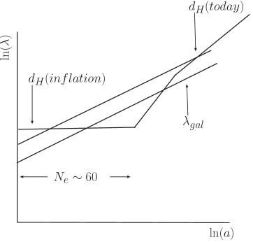
Figure 6: Logarithm of physical scales vs. logarithm of the scale factor. The causal horizon $d_{H}$ is shown for the inflationary (De Sitter), radiation dominated and matter dominated stages. The physical wavelengths for today’s Hubble radius $d_{H}(today)$, and a galactic scale $\lambda_{gal}$ are shown.

This is the main concept behind the inflationary paradigm for the generation of temperature fluctuations as well as for providing the seeds for large scale structure formation: quantum fluctuations generated early in the inflationary stage exit the Hubble radius during inflation, and eventually re-enter during the matter dominated era. The basic mechanism for generation of temperature anisotropies as well as primordial gravitational waves through inflation is the followingbookkolb -muk : the energy momentum tensor is split into a the fluid component $T^{\mu\nu}_{fluid}$ [eq.(5)] that drives the classical FRW metric plus small quantum fluctuations, namely $T^{\mu\nu}=T^{\mu\nu}_{fluid}+\delta\,T^{\mu\nu}$ the quantum fluctuation of the matter fields induce a quantum fluctuation in the metric (geometry) $\delta\,G^{\mu\nu}=\delta\,T^{\mu\nu}/M^{2}_{Pl}$. In the linearized approximation the different wavelengths of the perturbations evolve independently. After a given wavelength exits the Hubble radius, the corresponding perturbation becomes causally disconnected from microphysical processes. Perturbations that re-enter the Hubble radius at the time of photon decoupling, about $400000$ years after the beginning of the Universe, induce small fluctuations in the space time metric which induce fluctuations in the matter distribution driving acoustic oscillations in the photon-baryon fluid. At the last scattering surface, when photons decouple from the plasma these oscillations are imprinted in the power spectrum of the temperature anisotropies of the CMB and seed the inhomogeneities which generate structure upon gravitational collapsedodelson ; hu . The horizon problem, namely why the temperature of the CMB is nearly homogeneous and isotropic (to one part in $10^{5}$) is solved by an inflationary epoch because the wavelengths corresponding to the Hubble radius at the time of recombination were inside the Hubble radius hence in causal contact during inflation. This mechanism is depicted in fig. 6. While there is a great diversity of inflationary models, they generically predict a gaussian and nearly scale invariant spectrum of (mostly) adiabatic scalar (curvature) and tensor (gravitational waves) primordial fluctuations. These generic predictions of inflationary models make the inflationary paradigm robust. The gaussian, adiabatic and nearly scale invariant spectrum of primordial fluctuations provide an excellent fit to the highly precise wealth of data provided by the Wilkinson Microwave Anisotropy Probe (WMAP)WMAP1 ; kogut ; spergel ; peiris . WMAP has also provided perhaps the most striking validation of inflation as a mechanism for generating superhorizon fluctuations, through the measurement of an anticorrelation peak in the temperature-polarization (TE) angular power spectrum at $l\sim 150$ corresponding to superhorizon scaleskogut ; spergel ; peiris .

IV.2 Inflation and scalar field dynamics

A simple implementation of the inflationary scenario is based on a single scalar field, the inflaton with a Lagrangian density

$$\mathcal{L}=a^{3}(t)\left[\frac{\dot{\varphi}^{2}}{2}-\frac{(\nabla\varphi)^{2}}{2a^{2}(t)}-V(\varphi)\right]$$ (30)

with $V(\varphi)$ the inflationary potential. The energy density and the pressure for a spatially homogeneous and isotropic inflaton $\varphi(t)$ field in the early universe [see sec. II.2] are given by bookkolb -liddlerev

$$\rho=\frac{\dot{\varphi}^{2}}{2}+V(\varphi)\quad,\quad p=\frac{\dot{\varphi}^{2}}{2}-V(\varphi)\;.$$ (31)

Inflation should last at least $N_{e}\gtrsim 60$ efolds in order to solve the entropy and horizon problems. This entails a slow evolution and small temporal derivatives for the inflaton (slow roll), namely $\dot{\varphi}^{2}\ll V(\varphi)$. This implies $\rho=-p\simeq V(\varphi)\simeq{\rm constant}$ as the equation of state leading to a de Sitter universe with scale factor $a(t)=e^{Ht},\;H=\sqrt{V(\varphi)/[3\;M^{2}_{Pl}]}$ [see eq. (11)]. This situation is achieved via a variety of inflationary scenarios, old, new, chaotic, hybrid inflation etc. (see bookkolb -muk for discussions on different models).

While inflationary dynamics is typically studied in terms of a classical homogeneous inflaton field, such classical field must be understood as the expectation value of a quantum field in an isotropic and homogeneous quantum state. In ref.classi ; tsu the quantum dynamics of inflation was studied for inflation potentials which features a discrete symmetry breaking, $V(\varphi)=-m^{2}\varphi^{2}/2+\lambda\varphi^{4}$ (new inflation) as well as unbroken symmetry potentials $V(\varphi)=+m^{2}\varphi^{2}/2+\lambda\varphi^{4}$. The initial quantum state was taken to be a gaussian wave function(al) with vanishing or non-vanishing expectation value of the field. This state evolves in time with the full inflationary potential which features a spinodal region for $\varphi^{2}<m^{2}/12\lambda$ in the broken symmetric case. Just as in the case of Minkowski space time, there is a band of spinodally or parametrically unstable wave vectors, within this band the amplitude of the quantum fluctuations grows. Because of the cosmological expansion wave vectors are redshifted into the unstable band and when the wavelength of the unstable modes becomes larger than the Hubble radius these modes become classical with a large amplitude and a frozen phase. These long wavelength modes assemble into a classical coherent and homogeneous condensate, which obeys the equations of motion of the classical inflatonclassi ; tsu . This phenomenon of classicalization and the formation of a homogeneous condensate takes place during the first $5-10$ e-folds after the beginning of the inflationary stage. The full quantum theory treatment in refs.classi ; tsu show that this rapid redshift and classicalization justifies the use of an homogeneous classical inflaton leading to the following robust conclusionsclassi ; tsu :

• The quantum fluctuations of the inflaton are of two different kinds: (a) Large amplitude quantum fluctuations generated at the begining of inflation through spinodal or parametric resonance depending on the inflationary scenario chosen. They have comoving wavenumbers in the range of $e^{N_{T}-60}\;10^{13}\mbox{GeV}\lesssim k\lesssim e^{N_{T}-60}\;10^{15}$ GeV and they become superhorizon a few efolds after the begining of inflation. The phase of these long-wavelength fluctuations freeze out and their amplitude grows thereby effectively forming a homogeneous classical condensate. The study of more general initial quantum states featuring highly excited distribution of quanta lead to similar conclusionstsu : during the first few e-folds of evolution the rapid redshift results in a classicalization of long-wavelength fluctuations and the emergence of a homogeneous coherent condensate that obeys the classical equations of motion in terms of the inflaton potential. (b) Cosmological scales relevant for the observations today between $1\,\textrm{Mpc}$ and the Hubble radius had first crossed (exited) the Hubble radius about $\sim 50$ e-folds before the end of inflation within a rather narrow window of about $8$ e-foldsbookkolb . These correspond to small fluctuations of high comoving wavevectors in the rangedodelson $e^{N_{T}-60}\;10^{16}\,GeV<k<e^{N_{T}-60}\;10^{20}\,GeV$ where $N_{T}\geq 60$ is the total number of efolds.

• During the rest of the inflationary stage the dynamics is described by this classical homogeneous condensate that obeys the classical equations of motion with the inflaton potential. Thus inflation even if triggered by an initial quantum state or density matrix of the quantum field, is effectively described in terms of an homogeneous scalar condensate.

The body of results emerging from these studies provide a justification for the description of inflationary dynamics in terms of classical homogeneous scalar field. The conclusion is that after a few initial e-folds during which the unstable wavevectors (a) are redshifted well beyond the Hubble radius, all that remains for the ensuing dynamics is an homogeneous condensate, plus small fluctuations corresponding to modes (b).

IV.3 Slow roll inflation

Amongst the wide variety of inflationary scenarios, slow roll inflationbarrow ; stewlyth provides a simple and generic description of inflation consistent with the WMAP datapeiris . In this scenario, inflation is driven by the dynamics of the classical coherent and homogeneous condensate of the inflaton field $\varphi(t)$, which obeys the classical equation of motion

$${\ddot{\varphi}}+3\,H\,{\dot{\varphi}}+V^{\prime}(\varphi)=0\;.$$ (32)

Its energy density is given by $\rho(t)=\frac{{\dot{\varphi}}^{2}}{2}+V(\varphi)$. The basic premise of slow roll inflation is that the potential is fairly flat during the inflationary stage. This flatness not only leads to a slowly varying inflaton and Hubble parameter, hence ensuring a sufficient number of e-folds, but also provides an explanation for the gaussianity of the fluctuations as well as for the (almost) scale invariance of their power spectrum. A flat potential precludes large non-linearities in the dynamics of the fluctuations of the inflaton, which is therefore determined by a gaussian free field theory. Furthermore, because the potential is flat the inflaton is almost massless (compared with the scale of $V^{\frac{1}{4}}$), and modes cross the horizon with an amplitude proportional to the Hubble parameter. This fact combined with a slowly varying Hubble parameter yields an almost scale invariant primordial power spectrum. Departures from scale invariance and gaussianity are determined by the departures from flatness of the potential, namely by derivatives of the potential with respect to the inflaton field. These derivatives are small and can be combined into a hierarchy of dimensionless slow roll parametersbarrow that allow an assessment of the corrections to the basic predictions of gaussianity and scale invariancepeiris . The slow roll expansion introduces a hierarchy of small dimensionless quantities that are determined by the derivatives of the potentialbarrow ; stewlyth :

$$\epsilon_{V}=\frac{M^{2}_{Pl}}{2}\;\left[\frac{V^{{}^{\prime}}(\varphi)}{V(\varphi)}\right]^{2}~{},~{}\eta_{V}=M^{2}_{Pl}\;\frac{V^{{}^{\prime\prime}}(\varphi)}{V(\varphi)}~{},~{}\xi_{V}=M^{4}_{Pl}\;\frac{V^{\prime}(\varphi)\;V^{{}^{\prime\prime\prime}}(\varphi)}{V^{2}(\varphi)}\;.$$ (33)

The slow roll approximationbarrow ; bookliddle ; stewlyth corresponds to $\epsilon_{V}\sim\eta_{V}\ll 1$ with the hierarchy $\xi_{V}\sim\mathcal{O}(\epsilon^{2}_{V})$, namely $\epsilon_{V}$ and $\eta_{V}$ are first order in slow roll, $\xi_{V}$ second order in slow roll, etc. The slow roll variable $\epsilon_{V}\ll 1$ implies that the evolution of the inflaton $\varphi$ is slow, and to leading order (neglecting the second derivatives), the equation of motion (32) becomes

$$3H(t)~{}\dot{\varphi}+V^{\prime}(\varphi)=0$$ (34)

with

$$H^{2}(t)=\frac{V(\varphi)}{3M^{2}_{Pl}}\;.$$ (35)

The second slow roll variable $\eta_{V}\ll 1$ implies that the inflationary potential is nearly flat during the inflationary stage. During slow roll inflation the number of e-folds, from the time $t$ till the end of inflation, at which the value of the inflaton is $\varphi_{e}$, is given by

$$N_{e}[\varphi(t)]=-\frac{1}{M^{2}_{Pl}}\int^{\varphi_{e}}_{\varphi(t)}\frac{V(\varphi)}{V^{\prime}(\varphi)}\;d\varphi\;.$$ (36)

Small fluctuations of the scalar (matter) fields around the classical inflaton lead to small fluctuations in the space-time geometry through Einstein’s equations. There are two types fluctuations that are relevant: curvature perturbations and gravitational waves, both are produced during inflation. The fluctuations of the scalar field generate directly fluctuations in the curvature of space-time, while the expansion of the Universe, itself determined by the dynamics of the scalar field generates gravitational waves (see refs.dodelson ; hu ). In the linearized approximation different wavevectors of the fluctuations evolve differently, the power spectra per logarithmic wave vector interval for curvature ($R$) and gravitational wave ($h$) fluctuations are respectively given by

$$\Delta^{2}_{R}(k)=\frac{k^{3}}{2\pi^{2}}\langle|R_{k}|^{2}\rangle~{}~{},~{}~{}\Delta^{2}_{h}(k)=\frac{k^{3}}{\pi^{2}}\langle|h_{+k}|^{2}+|h_{\times,k}|^{2}\rangle\;,$$ (37)

where the $R_{k}$ are the quanta of curvature fluctuations, $h_{+,\times}$ are the two independent polarizations of the quanta of gravitational waves, and the expectation value is in the vacuum state during inflation. These power spectra feature power laws in the slow roll regime,

$$\Delta^{2}_{R}(k)=\Delta^{2}_{R}(k_{0})\left(\frac{k}{k_{0}}\right)^{n_{s}-1}\quad,\quad\Delta^{2}_{h}(k)=\Delta^{2}_{h}(k_{0})\left(\frac{k}{k_{0}}\right)^{n_{T}}\;,$$ (38)

namely during slow roll the power spectra of curvature and gravitational wave perturbations are nearly scale invariant. The amplitude of the curvature perturbations for wavelengths that re-entered the Hubble radius at the last scattering surface are directly relatedbookkolb ; bookliddle to the temperature anisotropies measured by COBE and WMAPCOBE ; WMAP1 -peiris ,

$$\Delta_{R}=\left.\frac{4}{5}\frac{\Delta T}{T}\right|_{WMAP}=(4.67\pm 0.27)\times 10^{-5}$$ (39)

The amplitude and the power laws are determined in slow roll by

$$\Delta^{2}_{R}(k_{0})=\frac{V(\varphi)}{24\,\pi^{2}\;M^{4}_{Pl}\,\epsilon_{V}}~{}~{};~{}~{}\frac{\Delta^{2}_{h}(k_{0})}{\Delta^{2}_{R}(k_{0})}=16\;\epsilon_{V}~{}~{};~{}~{}n_{s}-1=-6\;\epsilon_{V}+2\;\eta_{V}~{}~{};~{}~{}n_{T}=-2\;\epsilon_{V}\;.$$ (40)

The WMAP values are for $k_{0}=0.002/\textrm{Mpc}$, which yields an upper bound for the scale of the inflationary potential during slow roll inflation $V^{1/4}<3.3\times 10^{16}\textrm{GeV}$, suggesting a connection between the scale of grand unification and that of inflation. While inflation may not be related to phase transitions in the early Universe, the nearly scale invariant spectrum of gaussian fluctuations suggests a connection with a critical theory. Ref. hectornorma provided an effective field theory description of inflation akin to the Landau-Ginzburg description of critical phenomena. Slow roll dynamics can be organized elegantly in a systematic expansion in powers of $1/N_{e}$ within a Landau-Ginzburg effective field theory. This is achieved by introducing a dimensionless inflaton field and rescaled potential as

$$\chi=\frac{\varphi}{\sqrt{N_{e}}M_{Pl}}$$ (41)

and

$$w(\chi)=\frac{V(\varphi)}{N_{e}\;M^{4}}$$ (42)

where the value of $\Delta_{R}$ [eq.(39)] and eq.(40) fix the scale of inflation $M$ to be $M\sim 10^{16}$ GeV and $N_{e}\sim 50$ is the number of e-folds. To emphasize that the slow roll approximation implies a slow time evolution it is also convenient to introduce a stretched (slow) dimensionless time variable $\tau$ and a rescaled dimensionless Hubble parameter $\hat{h}$ as follows

$$t=\sqrt{N_{e}}\;\frac{M_{Pl}}{M^{2}}\;\tau\qquad;\qquad H=\sqrt{N_{e}}\;\frac{M^{2}}{M_{Pl}}\;\hat{h}$$ (43)

the Einstein-Friedman equation now reads

$$\hat{h}^{2}(\tau)=\frac{1}{3}\left[\frac{1}{2\;N_{e}}\left(\frac{d\chi}{d\tau}\right)^{2}+w(\chi)\right]$$ (44)

and the evolution equation for the inflaton field $\chi$ is given by

$$\frac{1}{N_{e}}\;\frac{d^{2}\chi}{d\tau^{2}}+3\;\hat{h}\;\frac{d\chi}{d\tau}+w^{\prime}(\chi)=0$$ (45)

The slow-roll approximation follows by neglecting the $1/{N_{e}}$ terms in eqs.(44) and (45). Both $w(\chi)$ and $\hat{h}(\tau)$ are of order $N^{0}_{e}$ for large $N_{e}$. Both equations make manifest the slow roll expansion as a systematic expansion in $1/N_{e}$hectornorma ; mangano . Slow roll dynamics, the inflationary scale and all of the observational phenomenology is reproduced with $\chi\sim\mathcal{O}(1),\;w(\chi)\sim\mathcal{O}(1)$ during inflation.

As a pedagogical example for slow roll inflation we display the main features of the inflationary dynamics for $w(\chi)=(\chi^{2}-4)^{2}/16$ in fig.7. These figures reveal clearly that inflation ends at $\tau\sim 10$ when $\hat{h}(\tau)$ begins a rapid decrease when the field is no longer slowly coasting along near the maximum of the potential $\chi\sim 0$ but rapidly approaching its equilibrium minimum. The left panel $\ln a(\tau)$ depicts the number of e-folds as a function of time [by definition $N_{e}(t)=\ln a(t)$], wavelengths of cosmological relevance today have crossed the Hubble radius during the last $\sim 50$ e-folds before the end of inflation within a narrow window $\Delta N_{e}\sim 8$, corresponding to a very small interval $\Delta\tau\sim 1$. A successful inflationary scenario requires at least $N_{e}\sim 60$ to solve the horizon and entropy problems of the standard hot Big Bangbookkolb which occur in an interval $\Delta\tau\sim 3$ prior to the end of inflation and during which the dimensionless field changes about $\Delta\chi\sim 1$. These are general aspects of a wide range of inflationary scenariihectornorma .

Figure 7: Left panel: $\ln a(\tau)$ which is the number of e-folds as a function of time. Middle panel $\hat{h}(\tau)$. Right panel: $\chi(\tau)$ for $N_{e}=60$.

We consider here a translationally and rotationally invariant cosmology where the only source of inhomogeneities are (small) quantum fluctuations. Indeed, inhomogeneities cannot be excluded at the beginning of inflation but the redshift of scales during inflation by at least $e^{60}\sim 10^{26}$ effectively erases all eventual initial inhomogeneities.

Inflation is now an established part of cosmology with several important aspects, such as the superhorizon origin of density perturbations, having been spectacularly validated by WMAPpeiris . Simple but phenomenologically accurate descriptions of inflation invoke an effective field theory for a homogeneous scalar field, akin to the Landau-Ginzburg description of critical phenomena described in section III.1 abovehectornorma . Analysis of the WMAP data puts very strongly pressure on the simple monomial $w(\chi)=G_{4}\;\chi^{4}$ at the $3\sigma$ levelpeiris ; afterWMAP1 and forthcoming observations of the CMB as the Planck satellite and others bear the promise of yielding precise information on the inflaton effective potential corresponding to the stage of inflation during which wavelengths of cosmological relevance today first crossed the Hubble radius during inflation (see peiris ; afterWMAP1 ; hectornorma for discussions of the lessons learned so far).

V The Electroweak scale: phase transitions and baryogenesis

There is a large body of observational evidence that suggests that the there is more matter than antimatter in the Universe up to scales of the order of the Hubble radiusdolgovmat ; trodden . The origin of this baryon asymmetry is one of the deep mysteries in particle physics and cosmology. The value of this asymmetry is quantified by the ratio

$$\eta=\frac{n_{b}-n_{\bar{b}}}{n_{\gamma}}$$ (46)

where $n_{b}$ ($n_{\bar{b}}$) is the baryon (antibaryon) density and $n_{\gamma}$ is the photon density. This is the only free input parameter that enters in nucleosynthesis calculations of the primordial abundance of light elementssteigman ; turnerBBN . The agreement between the WMAP resultsWMAP1 ; kogut ; spergel ; peiris and the most recent analysis of the primordial deuterium abundancekneller yields

$$\eta=(6.1\pm 0.3)\times 10^{-10}$$ (47)

What is the origin of this ratio? namely what is the microscopic mechanism responsible for baryogenesis?. The necessary conditions for successful baryogenesis were first identified and outlined by Sakharovsakharov :

• Baryon number violation.

• C and CP violation: unless these symmetries are violated in any process in which baryons are created and annihilated, the rates for baryon production equals that of the reverse reaction and no net baryon can be generated by these processes.

• Departure from equilibrium: in equilibrium the density matrix only depends on the Hamiltonian (and simultaneously commuting operators) which in all microscopic theories is invariant under CPT. Since the baryon number operator is odd under CPT, the expectation value of the baryon operator must vanish if the density matrix is that of equilibriumtrodden .

Notably, the standard model of particle physics has the main ingredients for baryogenesistrodden ; buch :

• $B+L$ violation in the standard model: Since the weak interactions only involve the left handed quark (baryon) and lepton currents there is a quantum mechanical anomaly in their conservation lawsthooft :

  $$\partial_{\mu}J^{\mu,B}=\partial_{\mu}J^{\mu,l}=\frac{N_{f}}{32\;\pi^{2}}\left[-g^{2}\;W^{a}_{\mu\nu}\widetilde{W}^{a,\mu\nu}+g^{\prime 2}\;B_{\mu\nu}\widetilde{B}^{\mu\nu}\right]$$ (48)

  where $N_{f}$ is the number of generations, $W,B$ are the field strength tensors for the $SU(2)$ and $U(1)$ gauge fields and $\widetilde{W}^{\mu\nu}=\epsilon^{\mu\nu\alpha\beta}\;W_{\alpha\beta}$ and similarly for $\widetilde{B}$. As a consequence of this anomaly the change in the baryon (and lepton) number is related to the change in the topological charge of the gauge field

  $$\Delta B=N_{f}\,\Delta N_{CS}~{}~{};~{}~{}N_{CS}=\frac{g^{2}}{32\pi^{2}}\int d^{3}x\;\epsilon^{ijk}\,\textrm{Tr}\left[W_{i}\;\partial_{j}W_{k}+\frac{2\,i\,g}{3}\;W_{i}\;W_{j}\;W_{k}\right]$$ (49)

  where $W_{i}$ is the $SU(2)$ gauge field and $N_{CS}$ is an integer that characterizes the topological structure of the gauge field configuration. Kuzmin, Rubakov and Shaposhnikovkuzi noticed that in the high temperature medium that prevailed in the early Universe there are non-perturbative field configurations, called sphalerons that induce transitions between gauge field configurations with different values of $N_{CS}$. The sphalerons lead to $B+L$ violating processes with transition rate per unit volume estimated to begamsphal $\Gamma_{sph}\sim\alpha^{5}\;T^{4}\;\ln(1/\alpha)$. This estimate for the transition rate suggests that sphaleron processes are in thermal equilibrium for $100\,\textrm{GeV}<T<10^{12}$ GeV.

• CP violation in the standard model Because only left handed quarks and leptons couple to the charged and neutral vector bosons that mediate the weak interactions, the standard model violates P maximally. However, CP violation is much more subtle and is the result of CP violating phases in the complex Cabibbo Kobayashi Maskawa mass matrix for quarks resulting from complex Yukawa couplings to the Higgs field. For $N_{f}$ generations of quarks and leptons there are $(N_{f}-1)(N_{f}-2)/2$ independent phases in the CKM mass matrix, and a non-zero value for any of these phases implies CP violation. For $N_{f}\geq 3$ there is at least one CP violating phase, hence the standard model, with $N_{f}=3$ does indeed have the possibility of CP violation. Experimentally CP violation is observed in the $K_{0}\,\bar{K}_{0}$ and $B\,\bar{B}$ systems.

• Non-equilibrium: as discussed above weak interaction processes are in LTE down to $T\sim 1\,\mathrm{MeV}$, therefore the only possibility for non-equilibrium is through a phase transition. Since the expansion rate of the Universe is much smaller than the weak interaction rate, it is very likely that a second order phase transition at the electroweak scale $T\sim 100\,\textrm{GeV}$ would occur in LTE, hence departure from equilibrium requires a strong first order phase transition. An estimate of the possibility and strength of a first order electroweak phase transition in the standard model is gleaned from a one loop calculation of the effective potential in the $SU(2)+$ Higgs model (i.e, neglecting the $U(1)$ gauge group)trodden

  $$V^{(1)}(\varphi;T)=\left(\frac{3g^{2}}{32}+\frac{\lambda}{4}+\frac{m^{2}_{t}}{4v^{2}_{0}}\right)(T^{2}-T^{2}_{*})\;\varphi^{2}-\frac{3g^{2}}{32\pi}\,T\,\varphi^{3}+\frac{\lambda}{4}\;\varphi^{4},$$ (50)

  where $\varphi=\sqrt{\phi^{*}\phi},\;v_{0}$ is the Higgs vacuum expectation value at $T=0$ and $m_{t}$ is the top quark mass. The second term proportional to $\varphi^{3}$ arises from the gauge field contribution and is responsible for a first order phase transition. Including the $U(1)$ gauge group changes the above only quantitatively. The one loop effective potential as a function of $\varphi$ has a typical shape as in the right panel in fig. 2 and features a global and a local minimum fortrodden

  $$T<T_{c}=m_{H}\left(\frac{3g^{2}}{8}+\lambda-\frac{9g^{6}}{256\pi^{2}}+\frac{m^{2}_{t}}{v^{2}_{0}}\right)^{-\frac{1}{2}}$$ (51)

  where $m_{H}$ is the Higgs mass. A measure of the strength the phase transition is the ratio $\Delta\varphi(T_{c})/T_{c}$shapo where $\Delta\varphi(T_{c})$ is the jump in the order parameter between the two (degenerate) minima at $T_{c}$. Successful baryogenesis requires this ratio to be $>1$shapo . One important aspect that emerges from this simple analysis is that the higher the Higgs mass the weaker the phase transition. A study of higher ordersbuchfod reveals that perturbation theory does not give reliable information about the electroweak phase transition for Higgs masses beyond $\sim 70$ GeV. Lattice studies have shownjansen that the ratio $\Delta\varphi(T_{c})/T_{c}<1$ for $m_{H}>45\,\textrm{GeV}$. If the standard model features a strong first order phase transition this phase transition occurs via the formation of nucleated bubbles just as described in section III.2. Finally, a mechanism for baryogenesis involves transport of baryons through the bubble walls as the nucleated bubbles grow and percolate filling the space with the globally stable phasekaplan : CP violating interactions of quarks and leptons in the thermal medium with the bubble walls leads to an excess of left handed quarks, which sphaleron transitions convert into a net baryon asymmetry. For a discussion of these mechanisms seetrodden and references therein.

Caveats: While the standard model features the main ingredients for successful baryogenesis, a substantial body of work has revealed that for a Higgs mass larger than about $72$ GeV there is no first order phase transition but a smooth crossover in the standard modellaine ; csikor . The current LEP bound for the standard model Higgs mass $m_{H}\gtrsim 115$ GeV, all but rules out the possibility of a strong first order phase transition and suggests a smooth crossover from the broken symmetry into the symmetric phase in the standard model. While it has become clear that the LEP bound on the Higgs mass precludes baryogenesis in the standard model, some supersymmetric extensions of the standard model with a stop lighter than the top may be able to explain the observed baryon asymmetrylaine ; csikor ; carena . An alternative scenario for baryogenesis proposes that a primordial asymmetry between leptons and antileptons or leptogenesis is responsible for generating the baryon asymmetryfuku ; buch . The leptogenesis proposal depends on the details of the origin of neutrino masses and remains a subject of ongoing study.

VI The QCD phase transition in the early Universe

One of the most spectacular epochs in the early Universe is the QCD transition, when quarks and gluons become confined in hadrons. In the early Universe the baryon asymmetry is very small [see eq. (47)], and at RHIC (and soon at LHC) it is expected that the mid-rapidity region for central collisions is also baryon free (see the discussion in section VIII.1 below). For the purpuse of cosmology, one would wish to directly measure $T_{QCD}$ and the equation of state from experiments with relativistic heavy ions, but it turns out not to be a simple task. The problem arises from extremely different time scales: $10^{-5}$ s in the cosmological QCD transition (very close to thermal equilibrium), but only $10^{-23}$ s in the laboratory (out-of-equilibrium effects may be important).

Since QCD is asymptotically free, it is expected that at high temperature a perturbative evaluation of the equation of state in terms of a weakly interacting gas of quark and gluons should be reliable. However near the hadronization phase transition the nature of the degrees of freedom changes from quarks and gluons to hadrons and QCD becomes non-perturbative. The only known first principle method to study QCD non-perturbatively in a wide temperature range is lattice gauge theory (LGT). Over the last several years there has been steady progress in the study of the QCD phase diagram with and without chemical potential including light and heavy quarks karsch2 ; Laermann:2003cv ; Katz:2005br . As explained above, the problems to incorporate a finite chemical potential in LGT (see Laermann:2003cv ) is of no concern to cosmology and the mid-rapidity region of central collisions at RHIC and LHC, because the relevant baryochemical potentials $\mu_{B}/T\ll 1$.

For an extended review of the cosmological consequences of the QCD transition and the physics of the first second of the Universe see Schwarz:2003du .

VI.1 The QCD transition and equation of state:

VI.1.1 Lattice gauge theory results

It has been established that lattice QCD without dynamical quarks (quenched approximation) exhibits a thermal first-order phase transition Fukugita:1989yb at a critical temperature of $T_{\star}\approx 270$ MeV Laermann:2003cv . This is also in agreement with the expectation of a first-order phase transition from the simplest bag model bagEOS ; teaney ; shuryak (see below). Unfortunately, the situation is not clear for dynamical quarks and is especially unclear for the physical values of the up, down and strange quark masses.

For dynamical quarks, lattice QCD calculations provide a range of estimates for $T_{c}$. In the case of two-flavour QCD $T_{c}\approx 175$ MeV AliKhan:2000iz ; Karsch:2000kv , whereas for three-flavour QCD $T_{c}\approx 155$ MeV Karsch:2000kv , almost independent of the quark mass. For the most interesting case of two light quark flavors (up and down) and the more massive strange quark, a value of $T_{c}\approx 170$ MeV has been obtained recently, both from standard Aoki:1998gi and improved Bernard:2004je staggered quarks. Accordingly, in the discussion that follows we adopt a transition temperature $T_{c}=170$ MeV, keeping in mind that the systematic uncertainty is probably of the order $10$ MeV.

The order of the phase transition and the value of $T_{c}$ is still under investigation. For massless quarks the theoretical expectation is a second order transition for two quark flavors and a first-order transition for three and more quark flavors Pisarski:1983ms . On the lattice, for two light quarks the results are inconclusive. The predicted universality class is not confirmed so far (see discussions in Laermann:2003cv ); most recent studies even claim to find hints for a first-order transition D'Elia:2005sy . For three flavours close to the chiral limit the lattice results clearly indicate that the phase transition is of first order (see Laermann:2003cv ), as expected from theory. Some older simulations suggested that this holds true for the physical case as well Iwasaki:1995yj . The latter result was obtained using the Wilson quark action, whereas results with standard Aoki:1998gi and improved Bernard:2004je staggered quarks indicate a crossover for the physical quark masses.

A microscopic description of phase transitions in QCD requires also a reliable assessment of the equation of state (EoS). Furthermore, as it will be described below, a hydrodynamic description of the space-time evolution in relativistic heavy ion collisions also requires knowledge of the equation of state at high temperature. The consensus that seems to be emerging is that for the physical masses of two light (up and down) and one heavier (strange) quark there is a sharp crossover between a high temperature gas of quark and gluon quasiparticles and a low temperature hadronic phase without any thermodynamic discontinuities. This is displayed in fig. 8 which summarize results from LGT for the energy density and pressure (both divided by $T^{4}$ to compare to a free gas of massless quarks and or gluons) as a function of $T/T_{c}$ karsch2 . The most recent simulations of the equation of state are reviewed in Katz:2005br .

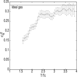
Figure 8: $\varepsilon/T^{4}$ and $p/T^{4}$, vs $T/T_{c}$ for a $16^{3}\times 4$ lattice From karsch2 . The arrows in the two left figures mark the Stephan-Boltzmann result. Right figure: speed of sound $C^{2}_{s}=\frac{dP}{d\varepsilon}$. From bernard

These figures clearly reveal a sharp decrease in the energy density and pressure at $T=T_{c}$, the value of the energy density is $\varepsilon_{c}\sim 6\;T^{4}_{c}$ karsch2 thus predicting an energy density $\varepsilon_{c}\sim 0.7\,\textrm{GeV}/\textrm{fm}^{3}$. Furthermore the high temperature behavior is not quite given by the Stephan-Boltzmann law, see fig. (8), suggesting that even at large temperatures the plasma is not described by free quarks and gluons up to temperatures $T\sim 4.0\;T_{c}\sim 700~{}{\rm Mev}$.

In the hydrodynamic limit, the speed of sound

$$c_{s}\equiv\left(\frac{\partial p}{\partial\epsilon}\right)_{S}^{1/2}$$ (52)

is a quantity of central interest. A strong decrease in the speed of sound, already above $T_{c}$, has been observed in lattice QCD, see bernard ; Aoki:2005vt for the most recent data. Consistent with previous results from quenched QCD and two-flavor QCD, $c_{s}^{2}(T_{c})\approx 0.1$ when approaching the critical temperature from above (in the QGP). The right panel of fig. 8 displays the speed of sound $c^{2}_{s}$ bernard clearly showing a dramatic decrease for $T\lesssim 2\;T_{c}$ and approaching $1/3$ for $T\gg T_{c}$ in agreement with an ultrarelativistic gas of quarks and gluons.

VI.1.2 The bag EOS and a first order phase transition

If the transition from $T>T_{c}$ to $T<T_{c}$ is continuous but sharp as evidenced by the lattice data in fig. 8 the behavior may not be too different from an actual transition which may be modelled by a simpler (EoS) which would allow an analytic treatment and to be included in a hydrodynamic description. The bag modelbagEOS provides a semi-phenomenological description of an (EoS) that features a quark-hadron transition. The simplest version considers the thermodynamics in two different regions: for $T>T_{c}$ a gas of massless quarks and gluons and confinement is accounted for in terms of a bag constant $B$bagEOS , for $T<T_{c}$ a gas of free massless pions (in the chiral limit). At $T=T_{c}$ quarks, gluons and pions coexist in equilibrium at constant pressure and temperature $p_{c},T_{c}$. In this model the pressure and energy density for vanishing chemical potential are given by

$$p_{>}=g_{>}\;\frac{\pi^{2}}{90}\;T^{4}-B~{}~{};~{}~{}\varepsilon_{>}=g_{>}\;\frac{\pi^{2}}{30}\;T^{4}+B~{}~{};~{}~{}\textrm{for}\;\,T>T_{c}\;,$$ (53)

$$p_{<}=g_{<}\;\frac{\pi^{2}}{90}\;T^{4}~{}~{};~{}~{}\varepsilon_{<}=g_{<}\;\frac{\pi^{2}}{30}\;T^{4}~{}~{};~{}~{}\textrm{for}\,T<T_{c}\;,$$ (54)

where $B$ is the bag constant with a typical value $B^{\frac{1}{4}}\sim 200$ MeVbagEOS . For a description of a quark-hadron transition $g_{>}=37,47.5$ for $N_{f}=2,3$ respectively and $g_{<}=3$ for a gas massless pions. The two regions are joined together by a flat coexistence curve with constant $p_{c},\;T_{c}$ according to a Maxwell construction (see sec.III.2.3). The value of $T_{c}$ is determined by this coexistence condition and is given by

$$T^{4}_{c}=\frac{90\;B}{(g_{>}-g_{<})\;\pi^{2}}\;\;.$$ (55)

For $N_{f}=2$ and three massless pions $T_{c}\sim 145$ Mev which is not too far from the lattice results $T_{c}\sim 170$ MeV. The flat coexistence region describes a mixed phase in which a quark-gluon plasma is in coexistence with a hadron gas with a vanishing isothermal sound speed, just like in the liquid-gas transition. The proportion of each phase in coexistence is determined by the lever-rule described in section III.2.3. The bag equation of state is therefore given by

$$p=\frac{\varepsilon}{3}-\frac{4}{3}\;B~{}~{};~{}~{}\textrm{for}~{}~{}\varepsilon>\varepsilon_{>}(T_{c})\quad,\quad p=\frac{\varepsilon}{3}~{}~{};~{}~{}\textrm{for}~{}~{}\varepsilon<\varepsilon_{<}(T_{c})\;,$$ (56)

with a flat coexistence line for $\varepsilon_{<}(T_{c})\leq p\leq\varepsilon_{>}(T_{c})$. This (EoS) is displayed in fig. 9, compare to the liquid-gas equation of state in the left panel of fig. 5.

Since the Helmholtz free energy density is $f(T)=\varepsilon-t\,s=-p$ with $s$ the entropy density, it is clear that for $T>T_{c}$ the free energy of the quark gluon phase is smaller and for $T<T_{c}$ the hadron phase has a smaller free energy. Since on the coexistence line $p=p_{c},\;T=T_{c}$ are constant, there is a jump in the entropy, namely a latent heat between the QGP and the hadronic phase, hence the bag model (EoS) leads to a first order phase transition with a latent heat

$$\textit{l}=T_{c}\;\Delta s=\varepsilon_{>}(T_{c})-\varepsilon_{<}(T_{c})=4\;B\;,$$ (57)

independent of the number of degrees of freedom. In the quenched approximation on the lattice, the latent heat was determined to be $l\approx 1.4\;T_{c}^{4}$ Iwasaki:1992ik ; Beinlich:1996xg , which is a factor of $5$ smaller than expected from a quenched bag model.

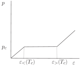
Figure 9: Bag (EoS) for a massless pion gas for $T<T_{c}$ and quarks and gluons in a bag for $T>T_{c}$.

More realistic versions of the bag equation of state have been constructed in ref.teaney ; shuryak . The importance of the bag (EoS) not only stems from its simplicity and the fact that it models a sharp crossover as evidenced by the lattice data but also because it is widely used in the hydrodynamic approach to ultrarelativistic heavy ion collisions [see the discussion in section VIII.1.1 below].

Besides the latent heat, the surface tension is the crucial parameter for the nucleation of bubbles in a first-order phase transition. The surface tension $\sigma\equiv\left({{\rm d}W}/{{\rm d}A}\right)_{V}$ is the work ${\rm d}W$ that has to be done per area ${\rm d}A$ to change the phase interface at fixed volume. The absence of surface excitations in hadronic spectra suggests that $\sigma^{1/3}\ll B^{1/4}$ Farhi:1984qu in the bag model. A self-consistent calculation of the surface tension within the bag model shows that the surface tension vanishes for massless quarks and gluons if no interactions besides the bag constant (i.e. $\alpha_{s}=0$) are taken into account Farhi:1984qu . This can be cured by introducing short-range interactions Farhi:1984qu or by including the strange quark mass Berger:1986ps ; Madsen:1994vp . For the surface tension rather small values are found from quenched lattice QCD, $\sigma\approx 0.015\;T_{c}^{3}$ Iwasaki:1993qu ; Beinlich:1996xg .

VI.2 Cosmological consequences of the QCD transition

In the radiation dominated Universe for $T>T_{c}$ the particle content is: quarks, gluons, leptons and photons. It is a good approximation to treat all particles with $m\ll 3\;T$ as massless. Above the QCD transition $g_{\rm quarks}=(7/8)12N_{f}$ (number of quark flavours) and $g_{\rm gluons}=8$, below the QCD transition $g_{\rm hadrons}$ quickly drops to zero, i.e. pions disappear at $T\sim 40$ MeV. Therefore at the QCD epoch $g_{>}=51.25\,(61.75)~{},~{}g_{<}=17.25(21.25)$ without (with) strange quarks and without (with) kaons, respectively. At the QCD transition the Hubble radius is about $10$ km, corresponding to scales of $1$ pc or $3$ light-years today. The mass inside a Hubble volume is $(4\pi/3)\;\epsilon(T_{c})\;R_{H}^{3}\sim 1M_{\odot}$. This mass is redshifted $\propto(1+z)$ as the Universe expands, because it is made up of radiation. The mass of cold dark matter in a comoving volume is invariant, $M_{\rm CDM}\equiv[(1+z_{\rm eq})/(1+z)]\;M(z)$. At the QCD transition $(1+z_{\rm eq})/(1+z)\sim 10^{-8}$ (recall $z_{\rm eq}\sim 10^{4}$), and thus

$$M_{\rm H}^{\rm CDM}\sim 10^{-8}M_{\odot}\ .$$ (58)

The Hubble time at the QCD transition, $t_{QCD}\sim 10^{-5}$ s, is much longer than the relaxation time scale of particle interactions. Thus, leptons, photons, the QGP and the hadron gas (HG) are in thermal and chemical equilibrium during cosmological time scales. All components are in LTE and form a radiation fluid. There conserved quantum numbers for this radiation fluid, lepton and baryon numbers (in the standard model). However, the corresponding chemical potentials are much smaller than the temperature at the QCD epoch. In this situation we can use the equation of state calculated in thermal lattice QCD and apply it directly to study the equilibrium aspects of cosmology. In standard cosmology, all lepton chemical potentials are assumed to vanish exactly. The baryon number density $n_{\rm B}$ follows from the ratio of baryons to photons at Big Bang Nucleosynthesis (BBN), $\eta\equiv(n_{\rm B}/n_{\gamma})_{\rm BBN}$, and the conservation of baryon number and entropy, $n_{\rm B}/s=$ constant:

$$n_{\rm B}(T_{c})=\eta\left(\frac{n_{\gamma}}{s}\right)_{\rm BBN}\;s(T_{c})=(8.2\pm 0.4)\times 10^{-11}\;s(T_{c})\;,$$ (59)

using the value of $\eta$ given in eq.(47). Finally, the baryon number inside a Hubble volume is given by

$$B_{\rm H}\approx\left(\frac{61.75}{g}\right)^{\frac{1}{2}}\;\left(\frac{170\mbox{\ MeV}}{T_{c}}\right)^{3}\;\left(\frac{\eta}{6.1\times 10^{-10}}\right)\;2.0\times 10^{48}$$ (60)

at the beginning of the transition and about twice that value at the end.

VI.2.1 A first-order QCD transition

If the cosmological QCD transition is of first order, it proceeds via bubble nucleation Hogan83 ; DeGrand . Its typical duration is $0.1t_{QCD}$. From the small values of surface tension and latent heat found in lattice QCD calculations Iwasaki:1993qu , the amount of supercooling is found to be small Ignatius . Hadronic bubbles nucleate during a short period of supercooling, $\Delta t_{\rm sc}\sim 10^{-3}\;t_{QCD}$. In a homogeneous Universe without ‘dirt’ the bubbles nucleate owing to thermal fluctuations (homogeneous nucleation), with a typical bubble nucleation distance of Christiansen

$$d_{\rm nuc}\sim 1\mbox{\ cm\ }\sim 10^{-6}\;R_{\rm H}\ .$$ (61)

The hadronic bubbles grow very fast, within $10^{-6}t_{QCD}$, until the released latent heat has reheated the Universe to $T_{c}$. By that time, just a small fraction of volume has gone through the transition. For the remaining $99\%$ of the transition, the HG and the QGP coexist at the pressure $p_{\rm HG}(T_{c})=p_{\rm QGP}(T_{c})$. During this time the hadronic bubbles grow slowly and the released latent heat keeps the temperature constant until the transition is completed. The energy density decreases continuously from $\epsilon_{\rm QGP}(T_{c})$ at the beginning of the transition to $\epsilon_{\rm HG}(T_{c})$ when the transition is completed.

In first-order phase transitions that we know from our everyday experience, like the condensation of water drops in clouds, the drops (bubbles) are nucleated at impurities (‘dirt’). This could happen in the early Universe as well. Candidates for cosmic ‘dirt’ are primordial black holes, monopoles, strings, and other kinds of defects. Of course, the existence of any of these objects has not been verified so far. Under these circumstances the typical nucleation distance may differ significantly from the scenario of homogeneous nucleation. For the QCD transition, heterogeneous nucleation has been studied in some detail in ref.Christiansen .

When the magnitude of primordial temperature fluctuations is of the same order or larger than the typical supercooling, the transition proceeds via inhomogeneous bubble nucleation. The mean nucleation distance results from the scale and amplitude of the temperature fluctuations.

Homogeneous nucleation : The probability to nucleate a bubble with critical radius (i.e. the minimal bubble size that can grow after its formation) by a thermal fluctuation per unit volume and unit time is given by (see discussion in Sec. III B.2)

$$I(T)=I_{0}(T)\;\exp\left(-\frac{\Delta W_{\rm c}}{T}\right)\ ,$$ (62)

with $\Delta W_{\rm c}=16\;\pi\;\sigma^{3}/[3\;(p_{\rm HG}-p_{\rm QGP})^{2}]$. For dimensional reasons $I_{0}\sim C\;T_{c}^{4}$, with $C={\cal O}(1)$. A more detailed calculation of $I_{0}$ within the bag model has been provided in Csernai . It was shown in Ref. Christiansen that the temperature dependence of the prefactor $I_{0}$ can be neglected for the calculation of the supercooling temperature $T_{\rm sc}$ in the cosmological QCD transition.

For small supercooling $\Delta\equiv 1-T/T_{c}\ll 1$ we may evaluate $(p_{\rm HG}-p_{\rm QGP})(T)$ by using the second law of thermodynamics, i.e. $p_{\rm HG}-p_{\rm QGP}\approx l\;\Delta$, and thus

$$I(\Delta)\approx I_{0}(T_{c})\;\exp\left(-A/\Delta^{2}\right),$$ (63)

with $A\equiv 16\;\pi\;\sigma^{3}/(3\;l^{2}\;T_{c})$ and $I_{0}(T_{c})\approx T_{c}^{4}$. Note that this result does not depend on the details of the QCD equation of state. For the values of $l=1.4\;T_{c}^{4}$ and $\sigma=0.015\;T_{c}^{3}$ from quenched lattice QCD Iwasaki:1993qu $A\approx 3\times 10^{-5}$. In the bag model $A\approx 5\times 10^{-2}\;(\sigma/T_{c}^{3})^{3}$.

The amount of supercooling that is necessary to complete the transition, $\Delta_{\rm sc}$, can be estimated from the schematic case of one single bubble nucleated per Hubble volume per Hubble time, which is

$${\cal O}(\Delta_{\rm sc})=\left[\frac{A}{4\;\ln(T_{c}/H_{QCD})}\right]^{1/2}\approx 4\times 10^{-4}$$ (64)

for the values of $l$ and $\sigma$ from quenched lattice QCD. For the bag model we assume $\sigma<0.1\;T_{c}^{3}$, which implies that $\Delta_{\rm sc}<6\times 10^{-4}$.

The time lapse during the supercooling period follows from the conservation of entropy and reads

$$\Delta t_{\rm sc}/t_{QCD}=\Delta_{\rm sc}/(3\;c_{s}^{2})={\cal O}(10^{-3})\ .$$ (65)

Here we used the relation $c_{s}^{2}={\rm d}\ln s/{\rm d}\ln T$ for the speed of sound in the supercooled phase. For realistic models $0<c_{s}(\Delta)<1/\sqrt{3}$, and in the bag model $c_{s}(\Delta)=1/\sqrt{3}$.

After the first bubbles have been nucleated, they grow most probably by weak deflagration DeGrand ; Kurki-Suonio ; Kajantie ; Ignatius . The deflagration front (the bubble wall) moves with the velocity $v_{\rm defl}\ll 1/\sqrt{3}$ Kajantie92 . The energy that is released from the bubbles is distributed into the surrounding QGP by a supersonic shock wave and by neutrino radiation. This reheats the QGP to $T_{c}$ and prohibits further bubble formation. Since the amplitude of the shock is very small Kurki-Suonio , on scales smaller than the neutrino mean free path, heat transport by neutrinos is the most efficient. Neutrinos have a mean free path of $10^{-6}R_{\rm H}$ at $T_{c}$. When they do most of the heat transport, heat goes with $v_{\rm heat}={\cal O}(c)$. For larger scales, heat transport is much slower. Figure 10 shows a sketch of the homogeneous bubble nucleation scenario.

Figure 10: Sketch of a first-order QCD transition via homogeneous bubble nucleation: above the critical temperature the Universe is filled with a quark–gluon plasma (Q). After a small amount of supercooling the first hadronic bubbles (H) nucleate at $t_{1}$, with mean separation $d_{\rm nuc}$. At $t_{2}>t_{1}$ these bubbles have grown and have released enough latent heat to quench the formation of new bubbles. The supercooling, bubble nucleation, and quenching takes just $1\%$ of the full transition time. In the remaining $99\%$ of the transition time the bubbles grow following the adiabatic expansion of the Universe. At $t_{3}$ the transition is almost finished. The shrinking QGP drops are separated by the typical distance $d_{\rm nuc}$.

Let us now calculate the mean bubble separation, $d_{\rm nuc}$, and the final supercooling, $\Delta_{\rm sc}$, for a scenario with weak deflagration. Bubbles present at a given time have typically been nucleated during the preceding time interval

$$\Delta t_{\rm nuc}\equiv I/({\rm d}I/{\rm d}t)\ .$$ (66)

Using the relation between time and supercooling, ${\rm d}\Delta/{\rm d}t=3\;c_{s}^{2}/t_{QCD}$, we find

$$\Delta t_{\rm nuc}/t_{QCD}=\Delta_{\rm sc}^{3}/(6\;A\;c_{s}^{2})={\cal O}(10^{-5})\quad\rm{and}\quad\Delta_{\rm nuc}=\frac{\Delta t_{\rm nuc}}{\Delta t_{\rm sc}}\;\Delta_{\rm sc}={\cal O}(10^{-2})\;\Delta_{\rm sc}\ .$$ (67)

During the time interval $\Delta t_{\rm nuc}$ each bubble releases latent heat, which is distributed over a typical distance $\approx 2\;v_{\rm heat}\;\Delta t_{\rm nuc}$. This distance has a weak dependence on the precise value of $\Delta_{\rm sc}$, but the bubble nucleation rate increases strongly with $\Delta$ until one bubble per volume $\sim(\Delta t_{\rm nuc}\;v_{\rm heat})^{3}$ is nucleated. Therefore the mean bubble separation is

$$d_{\rm nuc}\approx 2\;v_{\rm heat}\;\Delta t_{\rm nuc}\approx\frac{v_{\rm heat}}{3\;c_{s}^{2}}\;\frac{\Delta_{\rm sc}^{3}}{A}\;R_{\rm H}={\cal O}(10^{-6}\;R_{\rm H})={\cal O}(1{\rm cm}),$$ (68)

where we used $v_{\rm heat}={\cal O}(0.1),3\;c_{s}^{2}={\cal O}(0.1)$, which gives a typical value for the nucleation distance. The suppression of bubble nucleation due to already existing bubbles is neglected.

The estimate eq.(68) of the mean bubble separation applies if the released latent heat by means of sound waves and by neutrino free streaming is sufficient to reheat the QGP to $T_{c}$, i.e. to quench the nucleation of new bubbles. On the other hand the typical bubble separation could be given by the rate of release of latent heat, i.e. by the bubble wall velocity $v_{\rm defl}$. Since the period of supercooling lasts about $1\%$ of the time needed for completing the entire first-order phase transition, $1\%$ of the QGP must be converted to HG in the process of sudden reheating to $T_{c}$; the bubble radius at quenching must therefore reach $0.2$ of the bubble separation, $R_{\rm bubble}\approx 0.2\;d_{\rm nuc}$. With $R_{\rm bubble}\approx v_{\rm defl}\;\Delta t_{\rm nuc}$, and using the above relation $d_{\rm nuc}\approx 2\;v_{\rm heat}\;\Delta t_{\rm nuc}$, we require $v_{\rm defl}\geq 0.4v_{\rm heat}$ for consistency. If $v_{\rm defl}$ is smaller than this, the limiting factor for quenching is the rate of release of latent heat by bubble growth, and the bubble separation is

$$d_{\rm nuc}\approx 2\;v_{\rm defl}\;\Delta t_{\rm nuc}\approx\frac{v_{\rm defl}}{3\;c_{s}^{2}}\;\frac{\Delta_{\rm sc}^{3}}{A}\;R_{\rm H}\;,$$ (69)

i.e. the bubble separation will be smaller than the estimate in eq. (68).

We are now in a position to improve the estimate of $\Delta_{\rm sc}$: one bubble nucleates in the volume $(v_{\rm heat}\Delta t_{\rm nuc})^{3}$ during $\Delta t_{\rm nuc}$. This can be written as

$$1\approx(v_{\rm heat}\;\Delta t_{\rm nuc})^{3}\;\Delta t_{\rm nuc}I(t_{\rm sc})\ ,$$ (70)

which in terms of the supercooling parameter $\Delta_{\rm sc}$ is given by:

$$1\approx\frac{v_{\rm heat}^{3}}{(3\;c_{s}^{2}\;A)^{4}}\;\left(\frac{T_{c}}{H_{QCD}}\right)^{4}\;\Delta_{\rm sc}^{12}\;\exp\left(-\frac{A}{\Delta_{\rm sc}^{2}}\right)\approx 10^{94}\;\Delta_{\rm sc}^{12}\;\exp\left(-\frac{2.89\times 10^{-5}}{\Delta_{\rm sc}^{2}}\right)\;.$$ (71)

While the pre-exponential factor is smaller than the naive estimate eq.(64) by a factor of $10^{20}$, the amount of supercooling is just $20\%$ larger than in eq.(64), i.e. $\Delta_{\rm sc}=5\times 10^{-4}$, confirming, that that numerical prefactors in eq.(70) are irrelevant in the calculation of $\Delta_{\rm sc}$.

In summary, the scales on which non-equilibrium phenomena occur are given by the mean bubble separation, which is about $10^{-6}R_{\rm H}$. The entropy production is tiny, i.e. $\Delta S/S\sim 10^{-6}$, since the supercooling is small $\sim 10^{-3}$. After supercooling, which lasts $10^{-3}\;t_{QCD}$, the Universe reheats in $\Delta t_{\rm nuc}\approx 10^{-6}\;t_{QCD}$. After reheating, the thermodynamic variables follow their equilibrium values and bubbles grow only because of the expansion of the Universe.

Inhomogeneous nucleation: The local temperature $T(t,{\bf x})$ of the radiation fluid fluctuates, because cosmological perturbations have been generated during cosmological inflationhu . Let us denote the temperature fluctuation by $\Delta_{T}\equiv\delta T/T$. Inflation predicts a Gaussian distribution of perturbations (see sectionIV):

$$P(\Delta_{T})\;{\rm d}\Delta_{T}=\frac{1}{\sqrt{2\pi}\Delta_{T}^{\rm rms}}\exp\left[-\frac{1}{2}\frac{\Delta_{T}^{2}}{(\Delta_{T}^{\rm rms})^{2}}\right]{\rm d}\Delta_{T}\ .$$ (72)

If one allows for a tilt in the power spectrum of density fluctuations, the rms temperature fluctuation reads [see eq.(38) and ref.IS ],

$$\Delta_{T}^{\rm rms}\approx 10^{-4}\;(3\;c_{s}^{2})^{3/4}\;\left(\frac{k}{k_{0}}\right)^{(n_{s}-1)/2}\ ,$$ (73)

where $k_{0}$ is the wave number of the mode that crosses the Hubble radius today. For the scale-invariant spectrum ($n_{s}=1$) it is foundIS $\Delta_{T}^{\rm rms}(k_{\rm QCD})\approx 2\times 10^{-5}$.

The detailed analysis in ref.IS leads to the conclusion that the picture of homogeneous bubble nucleation, where bubbles form from statistical fluctuations, is false for the most probable cosmological scenarios.

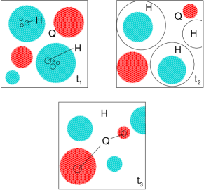
Figure 11: Sketch of a first-order QCD transition in the inhomogeneous Universe (from IS ): at $t_{1}$ the coldest spots (dark grey) are cold enough to render the nucleation of hadronic bubbles (H) possible, while most of the Universe remains in the quark–gluon phase (Q). At $t_{2}>t_{1}$ the bubbles from the cold spots have merged and have grown to bubbles as large as the fluctuation scale. Only the hot spots (light grey) are still in the QGP phase. At $t_{3}$ the transition is almost finished. The last QGP drops are found in the hottest spots of the Universe. The mean separation of these hot spots can be much larger than the homogeneous bubble nucleation separation.

A new scenario for the cosmological QCD transition was developed in ref.IS in which a small scale cut-off in the spectrum of primordial temperature fluctuations from collisional damping by neutrinos Weinberg ; SSW2 is included. This study revealed that at the QCD transition neutrinos travel freely on scales $\lambda_{\nu-{\rm mfp}}\approx 10^{-6}\;R_{\rm H}$, and that fluctuations on the diffusion scale of neutrinos are washed out by the time of the QCD transition:

$$\lambda_{\nu-{\rm diff}}=\frac{1}{3}\;\sqrt{\lambda_{\nu-{\rm mfp}}\;c\;t_{QCD}}\approx 10^{-4}\;R_{\rm H}\ .$$ (74)

Thus the old picture of homogeneous bubble nucleation still applies within the small homogeneous patches of $\lambda_{\rm smooth}=10^{-4}\;R_{\rm H}$.

The compression time scale for a homogeneous patch is $\delta t=\lambda_{\rm smooth}/c_{s}\sim 10^{-3}\;t_{QCD}$. If the compression time scale is larger than $\Delta t_{\rm nuc}$ the temperature fluctuations are frozen with respect to the time scale of nucleations.

A sketch of inhomogeneous bubble nucleation is shown in fig. 11. The basic idea is that temperature inhomogeneities determine the location of bubble nucleation. In cold regions, bubbles nucleate first. In general we have two possible situations:

1. If $\Delta_{\rm nuc}>\Delta_{T}^{\rm rms}$, the temperature inhomogeneities are negligible and the phase transition proceeds via homogeneous nucleation (see section VI.2.1).

2. If $\Delta_{\rm nuc}<\Delta_{T}^{\rm rms}$, the nucleation rate is inhomogeneous and we have to consider the scenario sketched in fig. 11.

A first attempt to analyse inhomogeneous nucleation has been given in IS . According to IS , the nucleation distance $d_{\rm nuc}$ exceeds the scale $\lambda_{\rm smooth}$, if

$$\lambda_{\rm smooth}<2\;\frac{v_{\rm heat}}{3\;c_{s}^{2}}\Delta_{T}^{\rm rms}\;R_{\rm H}.$$ (75)

If $\Delta_{T}^{\rm rms}>5\times 10^{-5}$, it is quite likely that this condition is met. In that case we can conclude that the typical inhomogeneity scale in the baryon distribution is inherited from the scale of density inhomogeneities in the radiation fluid at the end of the QCD transition. The effect in terms of length scales is at least two orders of magnitude larger than the nucleation distance in homogeneous nucleation and is ${\cal O}(1\mbox{\ m})$, which is of interest for inhomogeneous BBN.

VI.2.2 Effects from a first-order QCD transition

Let us now briefly summarize the effects that have been suggested to emerge from the cosmological QCD transition. There are two kinds of effects: the effects that have been found in the mid 80s and early 90s stem from the bubble scale and they thus affect scales $\lambda\leq d_{\rm nuc}$. The formation of quark nuggets, the generation of isothermal baryon fluctuations, the generation of magnetic fields and gravitational waves belong to the effects from the bubble scale.

In recent years it was found that there is another class of possible consequences from the QCD transition, which are connected to the Hubble scale and therefore affect scales $\lambda\leq R_{\rm H}$. Among these effects are the amplification of inhomogeneities and later formation of cold dark matter clumps, the modification of primordial gravitational waves, and the enhanced probability of black hole formation during the QCD transition.

Quark nuggets/Strangelets: In 1971 Bodmer Bodmer suggested the possibility that strange quark matter might be the ground state of bulk matter, instead of ⁵⁶Fe. Later Witten Witten rediscovered this idea. Strange quark matter was further studied by Farhi and Jaffe Farhi:1984qu . The idea of strange quark matter is based on the observation that the Pauli principle allows more quarks to be packed into a fixed volume in phase space if three instead of two flavours are available. Thus the energy per baryon would be lower in strange quark matter than in nuclei. However, the strange quark is heavy compared with up and down quarks, and this mass counteracts the advantage from the Pauli principle. No strange quark matter has been found experimentally so far smexp . The issue of stability of strange quark matter has not been settled yet; for a recent review see Madsen .

Witten Witten pointed out that a separation of phases during the coexistence of the hadronic and the quark phase could gather a large number of baryons in strange quark nuggets Witten . These quark nuggets could contribute to the dark matter today Witten or affect BBN steigman ; turnerBBN . At the end of the transition the baryon number in the quark droplets could exceed the baryon number in the hadron phase by several orders of magnitude, $n_{\rm B}^{\rm QGP}$ could be close to nuclear density. However, it was realized that the quark nuggets, while cooling, lose baryons. The quark nuggets evaporate as long as the temperature is above $\sim 50$ MeV Alcock . Quark nuggets may survive this evaporation if they contain much more than $\sim 10^{44}$ baryons initially evap . This number should be compared with the number of baryons inside a Hubble volume at the QCD transition, which is $10^{48}$. Thus, the mean bubble nucleation distance should be $>3\times 10^{-2}R_{\rm H}\sim 300$ m so as to collect enough baryons. This seems impossible from todays perspective, as explained above.

Inhomogeneous nucleosynthesis: Applegate and Hogan Applegate found that a strong first-order QCD phase transition induces inhomogeneous nucleosynthesis. It is extremely important to understand the initial conditions for BBN, because many of our ideas about the early Universe rely on the validity of the standard (homogeneous) BBN scenario. This is in good agreement with observations steigman ; turnerBBN . In inhomogeneous nucleosynthesis IBBN , large isothermal fluctuations of the baryon number (the remnants of the quark droplets at the end of the QCD transition) could lead to different yields of light elements. As a minimal requirement for an inhomogeneous scenario of nucleosynthesis, the mean bubble nucleation distance has to be larger than the proton diffusion length, which corresponds to $\sim 3$ m Mathews at the QCD transition. This is two orders of magnitude above recent estimates of the typical nucleation distance Christiansen .

Although values for $\eta$ dramatically different from those in the standard BBN are excluded both from measurements of the light element abundances and from the CMB, it might be possible to alter the primordial abundance of heavy elements ($A>7$) in inhomogeneous scenarios JedamzikHE .

Cold dark matter clumps: Scales $\lambda$ that are of the order of the Hubble radius $R_{\rm H}$ are not sensitive to details of the bubbles. It was reported in Refs. SSW ; SSW2 that the evolution of cosmological density perturbations (see Sec. III) is strongly affected by a first-order QCD transition for subhorizon scales, $\lambda<R_{\rm H}$.

In the radiation-dominated Universe subhorizon density perturbations perform acoustic oscillations. The restoring force is provided by pressure gradients. These, and therefore the speed of sound $c_{s}=\left(\partial p/\partial\epsilon\right)_{S}^{1/2}$ (on scales much larger than the bubble separation scale) drop to zero at a first-order QCD transition SSW , because both phases coexist at the pressure $p_{c}$ only ($a$ is the scale factor of the Universe):

$$c_{s}^{2}=\frac{{\rm d}p_{c}/{\rm d}a}{{\rm d}\epsilon(a)/{\rm d}a}=0\ .$$ (76)

It stays zero during the entire transition and suddenly rises back to the radiation value $c_{s}=1/\sqrt{3}$ after the transition. A significant decrease in the effective speed of sound $c_{s}$ during the cosmological QCD transition was also pointed out by Jedamzik Jedamzik .

As the speed of sound drops to zero, the restoring force for acoustic oscillations vanishes and density perturbations for subhorizon modes fall freely. The fluid velocity stays constant during this free fall. Perturbations of shorter wavelengths have higher velocities at the beginning of the transition, and thus grow proportional to the wave number $k$ during the phase transition. The primordial Harrison–Zel’dovich spectrum of density perturbations is amplified on subhorizon scales. The spectrum of density perturbations on superhorizon scales, $\lambda>R_{\rm H}$, is unaffected. At $T\sim 1$ MeV the neutrinos decouple from the radiation fluid. During this decoupling the large peaks in the radiation spectrum are wiped out by collisional damping Weinberg .

Today a major component of the Universe is dark matter, most likely CDM. If CDM is kinetically decoupled from the radiation fluid at the QCD transition, the density perturbations in CDM do not suffer from the neutrino damping. This is the case for primordial black holes or axions, but not for supersymmetric dark matter. At the time of the QCD transition the energy density of CDM is small, i.e. $\epsilon_{\rm cdm}(T_{c})\sim 10^{-8}\;\epsilon_{\rm rad}(T_{c})$. CDM falls into the potential wells provided by the dominant radiation fluid. Thus, the CDM spectrum is amplified on subhorizon scales. The peaks in the CDM spectrum go non-linear shortly after radiation–matter equality. This leads to the formation of CDM clumps with mass $<10^{-10}M_{\odot}$. Especially the clumping of axions has important implications for axion searches Sikivie . If the QCD transition is strong enough, these clumps could be detected by gravitational femtolensing femtolensing .

VI.2.3 Damping of gravitational waves at the QCD transition

In principle, primordial gravitational waves (e.g. from cosmological inflation) present a clean probe of the dynamics of the early Universe, since they know only about the Hubble expansion. As was shown in Schwarz a step is imprinted in the spectrum of primordial gravitational waves by the cosmological QCD transition. This step does not allow us to tell the difference between a first-order transition and a crossover, but an estimate of the transition temperature and a measurement of the drop in effective number of relativistic degrees of freedom would be possible.

Primordial gravitational waves are predicted to be generated during inflation Starobinskii and could be detected by observing the so-called B-mode (parity odd patterns) polarisation of the CMB. Inflation predicts an almost scale-invariant energy density per logarithmic frequency interval for the most interesting frequencies ($\sim 10^{-8}$ Hz for pulsar timing, $\sim 10^{-3}$ Hz for LISA, and $\sim 100$ Hz for LIGO and VIRGO) of the gravitational waves. The energy fraction in gravitational waves, per logarithmic interval in frequency $f$, is defined by

$$\Omega_{\rm gw}(f)\equiv f\;{{\rm d}\epsilon_{\rm gw}\over{\rm d}f}\;{1\over\epsilon_{\rm c}}\ .$$ (77)

Figure 12 shows the transfer function $\Omega_{\rm gw}(f)/\Omega_{\rm gw}(f\ll f_{QCD})$ from the cosmological QCD transition. The typical frequency scale is

$$f_{QCD}\approx 1.5\left(g\over 17.25\right)^{\frac{1}{2}}\;{T_{c}\over 170\mbox{\ MeV}}\;10^{-7}\mbox{\ Hz}\ ,$$ (78)

which corresponds to the mode that crosses the Hubble horizon at the end of the bag model QCD transition. Scales that cross into the horizon after the transition (l.h.s. of the figure) are unaffected, whereas modes that cross the horizon before the transition are damped by an additional factor $\approx 0.7$. The modification of the differential spectrum has been calculated for a first-order (bag model) and a crossover QCD transition. In both cases the step extends over one decade in frequency. The detailed form of the step is almost independent from the order of the transition.

Figure 12: The modification of the energy density, per logarithmic frequency interval, for primordial gravitational waves from the QCD transition (from Schwarz ).

The size of the step can be calculated analytically Schwarz . Comparing the differential energy spectrum for modes that cross into the horizon before and after the transition gives the ratio

$${\Omega_{\rm gw}(f\gg f_{QCD})\over\Omega_{\rm gw}(f\ll f_{QCD})}=\left(g_{\rm a}\over g_{\rm b}\right)^{\frac{1}{3}}\approx 0.696\ ,$$ (79)

for the QCD transition.

In fig. 12 we indicated the frequency range ($\sim 1$ yr^-1) in which limits on $\Omega_{\rm gw}$ have been reported from pulsar timing residuals pulsar . Unfortunately, today’s technology does not enable us to detect primordial gravitational waves at frequencies around $10^{-7}$ Hz, because their expected amplitude is too small.

VII Observing the early Universe: the earliest is the latest.

As discussed above, during the inflationary stage the acceleration of the scale factor is positive, while in the radiation or matter dominated eras it is negative. Eq.(29) shows that wavelengths grow faster than the Hubble radius during inflation but slower during radiation and matter dominated eras. Perturbations of cosmological relevance with wavelengths between our Hubble radius today to galactic scales exited the Hubble radius during a window of $\sim 5-8$ e-folds about $55$ e-folds before the end of inflation thus becoming causally disconnected from microphysics. Wavelengths relevant to CMB anisotropies re-entered at the time of recombination prior to photon decoupling. Therefore CMB anisotropies provide direct information about the inflationary stage. Contrary to this case, the wavelengths of quantum fluctuations produced inside the Hubble radius during the radiation or matter dominated eras are always inside the Hubble radius and are causally influenced by microphysical processes. Hence observable consequences of processes that occurred during these eras are generally indirect. The baryon asymmetry is perhaps a remnant of the the microphysics of the standard model (or extensions thereof) and perhaps the QCD phase transition left an observable footprint as discussed in secs.VI.2.2 and VI.2.3. The time scale between the QCD phase transition $\sim 10\mu\textrm{secs}$ and that of nucleosynthesis $\sim 200\,\textrm{secs}$ is very large on the scale of strong interactions $\sim 10^{-23}\,\textrm{secs}$ which tend to erase any potentially interesting signature. Thus CMB observations, $400000$ years after the Big Bang, provide a window into the earliest phenomena that took place during inflation, while microphysical processes within the standard model of particle physics occur much later, are causal all throughout the evolution, and interactions blur their observable signals. An important possible remnant of these phase transitions are primordial magnetic fields.

A variety of astrophysical observations including Zeeman splitting, synchrotron emission, Faraday rotation measurements (RM) combined with pulsar dispersion measurements (DM) and polarization measurements suggest the presence of large scale magnetic fieldscmp ; han . The strength of typical galactic magnetic fields is of the order $\sim\mu~{}G$cmp ; han and they are correlated on very large scales up to galactic or even larger reaching to scales of cluster of galaxies $\sim 1~{}\mbox{Mpc}$cmp . The origin of these large scale magnetic fields is still a subject of discussion. It is currently agreed that a variety of dynamo mechanisms are efficient in amplifying seed magnetic fields with typical growth rates $\Gamma\sim\mbox{Gyr}^{-1}$ over time scales $\sim 10-12$ Gyr cmp . There are different proposals for the origin of the initial seed at different stages in the history of the early Universe, in particular during inflation, and or phase transitionscmp . Primordial (hyper) magnetic fields may have important consequences in electroweak baryogenesisgrassoEW , Big Bang nucleosynthesis (seecmp ), the polarization of the CMBvarios via the same physical processes as Faraday rotation, and structure formationcmp ,otros . If the electroweak and/or the chiral phase transitions occurred out of equilibrium they could be a significant source of primordial magnetic fieldsmagne . Thus cosmic magnetic fields may be one of the few observational relics of primordial phase transitions. The study of the origin of cosmic magnetic fields is one of the key science projects of the forthcoming Square Kilometer Array (SKA)SKA .

VIII Studying phase transitions with accelerators

VIII.1 Ultrarelativistic heavy ion collisions: seeking the Quark Gluon Plasma

The program of ultra relativistic heavy ion collisions (URHIC) whose primary goal is to study the phase diagram of QCD began almost two decades ago with the fixed target heavy ion programs at the AGS at Brookhaven and the SPS at CERN. A summary of the results of these efforts mainly through the $Pb+Pb$ experiments at SPS-CERN provided compelling evidence in favor of the existence of a new state of matterheinz . The program continues at the Relativistic Heavy Ion Collider (RHIC) at BNL. Unlike the fixed target experiment SPS at CERN, RHIC is a collider experiment which currently studies $Au+Au$ collisions with center of mass energy $\sqrt{s}\sim 200{\rm AGev}$ and luminosity $\sim 10^{26}cm^{-2}s^{-1}$. The future ALICE (A Large Ion Collider Experiment) heavy ion program at LHC is expected to study $Pb+Pb$ collisions with c.m. energies up to $\sqrt{s}\sim 5{\rm ATev}$ and luminosities $\sim 10^{27}cm^{-2}s^{-1}$. In these collisions the heavy nuclei can be pictured in the CM frame as two Lorentz contracted pancakes. For $Au+Au$ collisions the size of each pancake in the direction transverse to the beam axis is about 7 fm. At RHIC and LHC energies most of the baryons are expected to be carried away by the receding pancakes (the fragmentation region) while in the region of the collision a large energy (density) is deposited in the form of quark pairs and gluons. At least two important mechanisms for energy deposition in the collision region are at work muharris ; blaizot ; shuryak ; qgpbooks : i) the establishment of a strong color electric field (flux tube) that eventually breaks up into quark-antiquark pairs when the energy in the field is larger than the pair production threshold and ii) the partons (quarks and gluons) inside the colliding nuclei interact and redistribute their energy geiger . An estimate of the energy deposited in the collision region has been provided by Bjorken bjorken

$$\epsilon=\frac{1}{\tau_{0}\pi R^{2}_{A}}\frac{dE_{T}}{dy}$$ (80)

with $\tau_{0}\sim 1{\rm fm}/c$, $R_{A}\sim 7{\rm fm}$ for Au and $dE_{T}/dy$ is the transverse energy per unit rapidity which is measured. Parton-parton scattering is expected to lead to thermalization on time scales $\sim 1\,{\rm fm}/c$  muharris ; blaizot . After the quark-gluon plasma achieves LTE, the evolution is conjectured to be described by hydrodynamic expansion hydro1 . As the QGP expands and cools, the temperature falls near the critical temperature and the confinement and chiral phase transitions occurmeyer . Upon further cooling the quark-gluon plasma hadronizes, the hadrons rescatter until the hadron gas is dilute enough that the mean free path is larger than the mean distance between hadrons. At this point hadrons freeze-out and stream out freely to the detectors from this last scattering or freeze-out surface. This picture is summarized in fig. 13 below.

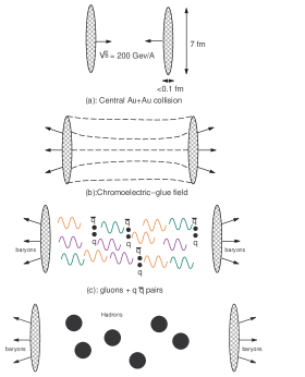
Figure 13: Heavy Ion Collisions.

Estimates based on this picture and on detailed numerical evolution evolutionqgp suggest that at RHIC the quark gluon plasma lifetime is of order $\sim 10fm/c$ while the total evolution until freeze-out is $\sim 50-100fm/c$.

VIII.1.1 Hydrodynamics, lattice gauge theory and the equation of state.

Although the evolution of the quark gluon plasma from the initial state described by the parton distribution of the colliding nuclei until freeze-out of hadrons clearly requires a non-equilibrium description, a hydrodynamic picture of the evolution is both useful and experimentally relevant hydro1 ; hydro2 . In the approximation in which quarks and gluons are strongly coupled in the sense that their mean free paths are much smaller than the typical wavelength for the variation of collective phenomena, the QGP can be described as a fluid in LTE, for which the energy momentum tensor is of the form

$$T^{\mu\nu}=(\varepsilon+p)\;u^{\mu}\;u^{\nu}-p\;g^{\mu\nu}\;,$$ (81)

with $\varepsilon,\;p$ the energy density and pressure respectively, $g^{\mu\nu}$ is the metric and

$$u^{\mu}=\gamma(x)\;(1,{\vec{v}}(x))$$ (82)

is a local 4-velocity vector with $\gamma(x)$ the local Lorentz contraction factor.

In this description the dynamical evolution of the fluid is obtained from the conservation laws of energy-momentum, baryon number and entropy shuryak ; qgpbooks ; meyer ; hydro1 with an equation of state $p=p(\varepsilon)$ to close the set of equations. A simple and phenomenologically useful description is provided by Bjorken’s model for longitudinal expansion shuryak ; qgpbooks ; bjorken ; hydro1 . There are three important ingredients in Bjorken’s models: i) the central rapidity region where the energy deposited and the formation of the QGP takes place well separated from the fragmentation region which is the region of the receding pancakes where most of the baryons are (see fig. 13). ii) The thermodynamic variables are invariant under boosts along the beam (longitudinal) axis, this is based on the observation that the particle distributions are invariant under these boosts in the central rapidity region and iii) the expansion only occurs along the beam axis, i.e, longitudinal expansion. In the baryon free region, local thermodynamics implies that the entropy density $s$ in the local rest frame of the fluid is related to the energy density $\varepsilon$ and pressure $p$ as

$$\varepsilon+p=T\;s\;.$$ (83)

It is convenient to introduce the space time rapidity $\eta$ and proper-time $\tau$ as

$$\eta=\frac{1}{2}\ln\left[\frac{t+z}{t-z}\right]~{}~{};~{}~{}\tau=\sqrt{t^{2}-z^{2}}\;,$$ (84)

with $z$ the coordinate along the beam axis (longitudinal) and the fluid rapidity $\theta$ by writing the local velocity eq.(82) as $u^{\mu}=(\cosh\theta,0,0,\sinh\theta)$. Bjorken’s model assumes the fluid to be composed of free streaming particles for which $v_{z}=z/t$ in which case the fluid rapidity $\theta$ becomes the space-time rapidity $\eta$. Boost invariance along the longitudinal direction entails that $\varepsilon,p,s,T$ are all functions of proper time onlybjorken ; hydro1 .

The energy-momentum conservation equation $\partial_{\mu}T^{\mu\nu}$ leads to two equations by projecting along the direction $u^{\mu}$ and perpendicular to it using the projector $g^{\mu\nu}-u^{\mu}u^{\nu}$. Under the assumption that the central region is baryon free, the conservation of entropy and energy and momentum lead to the following equations (for details see hydro1 ; meyer ; shuryak ; qgpbooks ; bjorken )

$$\frac{d\varepsilon(\tau)}{d\tau}+\frac{1}{\tau}(\varepsilon+p)=0\quad,\quad\frac{ds(\tau)}{d\tau}+\frac{s}{\tau}=0\;.$$ (85)

Assuming an equation of state $p(\tau)=p(\varepsilon(\tau))$ and combining eqs.(85) with the thermodynamic relation (83) (for baryon free plasmas) one finds that the evolution of the temperature is given by

$$\left.\frac{\tau}{T}\frac{dT}{d\tau}=-c^{2}_{s}\quad,\quad c^{2}_{s}=\frac{dP}{d\varepsilon}\right|_{s}\;.$$ (86)

Which for constant speed of sound results in the cooling law

$$T(\tau)=T_{0}\left(\frac{\tau_{0}}{\tau}\right)^{c^{2}_{s}}$$ (87)

Obviously, the form of eq.(85) is similar to the energy conservation equation (8) in cosmology with the expansion rate $\dot{a}/a=1/(3\tau)$ when the proper time $\tau$ is identified with the comoving time $t$ in the cosmological setting. The similarity becomes even more remarkable for the case of the QGP being modelled as a radiation fluid (which is expected to be a good approximation at high temperature) since in this case $c^{2}_{s}=1/3$ and the connection with a radiation dominated cosmology with scale factor $a(t)\propto t^{\frac{1}{3}}$ is evident.

To find the general evolution equations for the QGP, an equation of state is needed. It is at this stage where the connection with lattice gauge theory (LGT) is made. LGT obtains the thermodynamic functions in equilibrium and these are input in the hydrodynamic description as local functions of space-time under the assumption of LTE. However, practically hydrodynamic simulationshydro2 use a bag (EoS). For a discussion of the parameters in the bag (EoS) as well as a justification for using this equation of state which features a strong first order phase transition instead of the lattice (EoS) which features a crossover seehydro2 .

VIII.2 Predictions and observations pre-RHIC

Several experimental signatures had been associated with the formation of the QGP muharris ; signatures , and the heavy ion program at SPS focused on several of them. We summarize the observables that have been proposed as telltales of a QGP and the data gathered by the SPS from $Pb+Pb$ and $Pb+Au$ collisions, which taken together provide a hint of evidence heinz ; blaizot ; phystoday ; gyul for a QGP, although many of them could have alternative explanations.

VIII.2.1 $J/\Psi$ suppression and strangeness enhancement

The $J/\Psi$ is a narrow $\bar{c}c$ bound state, which, if produced in the early stages of the collision can probe the QGP because its lifetime is longer than that of the QGP and decays into dilepton pairs which leave the plasma without scattering. The original suggestion satz is that when the screening length of the color force is smaller than the size of the $\bar{c}c$ bound state, this narrow resonance will melt. This argument suggests that charmonium suppression could provide evidence for a QGP. Alternatively a suppression could result from scattering with hard gluons in the plasma and the dissociation of the bound state satz . A normal suppression of charmonium is expected on the grounds that once formed the $\bar{c}c$ bound state interact with other nucleons inside the nucleus. This expected suppression is studied in proton nucleon collisions and extrapolated to nucleon-nucleon collisions. This is considered the normal suppression in contrast to the abnormal suppression expected from the presence of a plasma. The left panel of fig. 14 shows the data gathered by the NA50 collaboration at the SPS-CERN jpsi .

This figure reveals an abnormal suppression when the energy density is $\varepsilon>2.5\,{\rm GeV}/{\rm fm}^{3}$. The energy density in this figure has been computed with Bjorken’s formula eq.(80). The NA50 collaboration at CERN-SPS jpsi2 combined data for $J/\Psi$ suppression from the NA38 and NA50 experiments. The analysis reveals that while for the most peripheral (largest impact parameter) collisions the suppression can be accounted for by nuclear absorption, there is no saturation in the suppression in the most central $Pb+Pb$ collisions and that the observed suppression pattern can be understood in a deconfinement scenario. This report concluded that the $J/\Psi$ suppression pattern observed in the NA50 data provides significant evidence for deconfinement of quarks and gluons in $Pb+Pb$ collisions. Strangeness enhancement along with chemical equilibration are some of the earliest proposals for clear signatures of the formation of a QGP strangeness . The main idea is based on the estimate that the strangeness equilibration time in a hot QGP is of the same order as the expected lifetime of the QGP ($\sim 10fm/c$) produced in nucleus-nucleus collisions. Two important aspects of this estimate make strangeness enhancement a prime candidate: if strangeness attains chemical equilibrium in the QGP, this equilibrium value is significantly higher than the strangeness production in nucleon-nucleon collisions. Also strangeness production through hadronic rescattering or final state interactions was estimated to be negligibly small strangeness . In the QGP, color deconfinement leads to a large gluon density that leads to the creation of $s\bar{s}$ pairs, furthermore chiral symmetry makes the strange quark lighter thus lowering the production threshold. This situation is in contrast to the case of hadronic rescattering or final state interactions where the production of pairs of strange quarks has large thresholds and small cross sections heinz . The usual measure of strangeness enhancement is through the ratio $\lambda_{s}={2\langle\bar{s}s\rangle}/{\langle\bar{u}u+\bar{d}d\rangle}$. The right panel in fig. 14 displays $\lambda_{s}$ as a function of $\sqrt{s}$ for nucleon-nucleon as well as nucleus-nucleus collisions ($S+S,S+Ag,Pb+Pb$) at SPS. The data displayed in fig. 14 is taken as evidence that nucleus-nucleus collisions at SPS are creating a hot state of matter.

Figure 14: Left panel: anomalous $J/\psi$ suppression as a function of the initial energy density. From jpsi . Right panel: The ratio $\lambda_{s}$ as a function of $\sqrt{s}$, the energy of the collision for nucleon-nucleon and nucleus-nucleus collisions. From soll

VIII.2.2 Electromagnetic probes: dileptons and direct photons

Electromagnetic probes: $e^{+}e^{-}$ or $\mu^{+}\mu^{-}$ dilepton pairs and direct (prompt) photons are prime probes of the hot plasma wam ; electro , since once produced they leave the plasma without further interactions because their mean free path is much larger than the typical size of the plasma. The $\rho$ vector meson is important because it decays into dileptons and its lifetime is $\sim 1fm/c$. Therefore once it is produced in the hadron gas it decays within the hot hadronic plasma and the produced dileptons carry direct information from the plasma. Thus while dileptons produced from the decay of the $\rho$ meson do not yield evidence of the earlier stages in the QGP, they do offer information on the hadronic stage. The left panel in fig. 15 presents the data gathered by the CERES-NA45 collaboration for the invariant mass spectrum for electron-positron pairs from 158 AGeV $Pb+Au$ collisions at the SPS-CERN. The solid line represents the expected spectrum from the decays of hadrons produced in proton-nucleon and proton-proton collisions extrapolated to $Pb+Au$ collisions and is the sum of the contributions shown in the graph. There are two remarkable features in this graph: a clear enhancement of dileptons in the region $2~{}{\rm MeV}\lesssim M_{e^{+}e^{-}}\lesssim 700~{}{\rm MeV}$ and that instead of the $\rho$ meson peak at $m_{\rho}=770~{}{\rm MeV}$ there is a broad distribution. The excess of dileptons in the small invariant mass region cannot be explained by charged pion annihilation heinz . It is remarkable that the dilepton enhancement is below the putative $\rho$ peak and that there is no hint of the $\rho$ at $770~{}{\rm MeV}$!. The current understanding of these features is that the medium effects result in a shift in the $\rho$ meson mass as well as a change in its widthwam ; heinz ; blaizot . Thus while this interpretation does not directly yield information on the QGP, it does support the picture of a hot gas of hadrons, mainly pions which is the main interaction channel of the $\rho$ vector meson. Direct photons are conceptually a clean direct probe of the early stages of the QGP. Photons are produced in the QGP by several processes: gluon-to-photon Compton scattering off (anti)quark $q(\bar{q})g\rightarrow q(\bar{q})\gamma$ and quark-antiquark annihilation to photon and gluon $q\bar{q}\rightarrow g\gamma$ and to the same order (see Kapusta et. al. and Aurenche et. al. in electro ) (anti)quark bremsstrahlung $qq(g)\rightarrow qq(g)\gamma$ and quark-antiquark annihilation with scattering $q\bar{q}q(g)\rightarrow q(g)\gamma$. Detailed calculations including screening corrections electro reveal that direct photons from the QGP could provide a signal that could be discriminated against the signal from the hadronic background. This work indicates the theoretical feasibility of direct photons as direct probes of the early stages of the QGP. The WA98 collaboration at SPS-CERN reported their analysis for the first observation of direct photons from $Pb+Pb$ collisions with $\sqrt{s}=158\,\textrm{AGeV}$ WA98 . Their data is summarized in the right panel of fig. 15. The transverse momentum distribution of direct photons is determined on a statistical basis and compared to the background photon yield predicted from a calculation of the radiative decays of hadrons. The most interesting result is that a significant excess of direct photons beyond that expected from proton-induced reaction at the same $\sqrt{s}\,$ is observed in the range of transverse momentum greater than about $1.5\;{\rm GeV}/c$ in central collisions. A comparison of the data to the theoretical predictions for direct photons from an equilibrated QGP was performed in ref hatsuda . The conclusions are that while it is not clear if SPS reached the energy density to form the QGP, the data indicates a hot and dense phase that could be its precursor. It has recently been shown wangnon that non-equilibrium effects in an expanding QGP formed in RHIC collisions lead to an enhancement of direct photons in the region of transverse momentum $p_{T}\gtrsim 2~{}{\rm GeV}$.

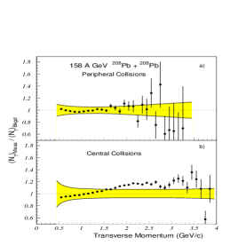
Figure 15: Left figure: invariant mass spectrum of $e^{+}e^{-}$ pairs from $Pb+Au$ collisions at 158 AGev at the SPS-CERN (CERES/NA45). From ceres . Right figure: ratio of total measured yield of direct photons to hadronic background vs. transverse momentum from $Pb+Pb$ at 158 AGev for peripheral and central collisions. From WA98 .

VIII.2.3 Quantum spinodal decomposition and pion domains

For massless up and down quarks, QCD has an $SU(2)_{L}\otimes SU(2)_{R}$ symmetry which is spontaneously broken down to $SU(2)_{L+R}$, this is the chiral phase transition. It has been argued that for massless quarks the equilibrium aspects of this transition is described by the universality class of the $O(4)$ Heisenberg ferromagnetraja . The Landau-Ginzburg effective field theory for this universality class is given by the effective potential

$$V(\vec{\Phi})=a\;(T-T_{c})\;\vec{\Phi}^{2}+g\;(\vec{\Phi}^{2})^{2}~{}~{};~{}~{}\vec{\Phi}=(\sigma,\vec{\pi})\;,$$ (88)

where $\sigma\sim\bar{\psi}\gamma^{5}\psi$ is the pseudoscalar chiral order parameter field that acquires an expectation value below the critical temperature, and $\vec{\pi}\sim\bar{\psi}\gamma^{5}\vec{\tau}\psi$ ($\tau^{a}=\textrm{isospin~{}matrices}$) is the triplet of pions, which are the Goldstone bosons associated with the symmetry breaking. In an URHIC, chiral symmetry is expected to be restored if a QGP is formed with $T>T_{c}$. Upon expansion and rapid cooling chiral symmetry is again broken. If the chiral phase transition occurs out of equilibrium, the ensuing quench can bring the hadronic phase into the spinodal region of the effective potential (88). As a result, quantum spinodal instabilities would lead to the formation of correlated domains inside which the order parameter is disoriented resulting in a disoriented chiral condensate(DCC)dcc ; raja . Spinodal instabilities would result in the formation and growth of pion domainsboydcc with distinct observational signatures in the pion distribution. A systematic study by the WA98 collaboration at SPS-CERNdccexp measured charged particle multiplicities in $158\,\textrm{AGeV}\,Pb+Pb$ collisions and ruled out the formation of (DCC) domains at $90\%\,CL$. The Minimax collaboration studied the possibility of (DCC)-like events at Fermilab’s Tevatron in $p\bar{p}$ collisionsminimax and found no statistically significant signals of large isospin fluctuations.

VIII.3 News from RHIC:

The four experiments at RHIC have presented their analysis of the first three years of operation at the top energy $\sqrt{s}=200A\,\textrm{GeV}$ for $Au+Au$ collisionsphenix . The combined body of results not only confirms most of the findings at SPS but also reveal novel and unexpected phenomenagyul ; phystoday . To begin with, the results on particle multiplicity when combined with Bjorken’s estimate for the value of the energy density eq.(80) yield $\varepsilon\sim 5.5\,\textrm{GeV}/\textrm{fm}^{3}$ for $\tau_{0}\sim 1\,\textrm{fm}/c$. This energy density is almost one order of magnitude larger than the critical value obtained from (LGT), $\varepsilon_{LGT}\sim 0.7\,\textrm{GeV}/\textrm{fm}^{3}$ (see section (VI.1.1)) therefore these experiments probe QCD in the deconfined regime. At least two important results stand out:

VIII.3.1 Elliptic flow, ideal hydrodynamics and early thermalization

If a QGP is formed early in the collision the pressure drives a collective expansion or flow. An important measure of this collective flow is elliptic flowolli in collisions with non-vanishing impact parameter (non-central). If the reaction plane is taken to be the $x-z$ plane, with $z$ the beam axis, the triple differential momentum distribution for hadron $h$ is expanded in a Fourier series in terms of the angle $\phi$ in the $x-y$ plane as

$$\frac{dN_{h}}{dydp_{T}^{2}d\phi}=\frac{dN_{h}}{2\pi\,dydp_{T}^{2}}\left[1+2v_{1}(y,p_{T})\cos\phi+2v_{2}(y,p_{T})\cos 2\phi+\cdots\right]\;\;.$$ (89)

The first coefficient $v_{1}$ vanishes at midrapidityhydro2 , the second $v_{2}$, the elliptic flow parameter is a measure of the hydrodynamic flow in peripheral collisions driven by pressure gradientshydro2 . A remarkable result from RHIC experiments is that ideal hydrodynamic calculations of $v_{2}$ are in excellent agreement with the combined experimental results from STARstarv2 and PHENIXphenixv2 for a many hadron species, up to $p_{T}\sim 2\,\textrm{GeV}$ as shown in fig. 16.

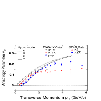
Figure 16: Combined STAR and PHENIX data on $v_{2}$. Fromphystoday .

A hydrodynamic calculation requires two inputs: an initialization (proper) time $\tau_{0}$ at which LTE is assumed to hold and an equation of state. The initial stage that leads to LTE requires knowledge beyond the realm of applicability of hydrodynamics. Hydrodynamic calculations just input initial data at a given (proper) time hypersurface. In most hydrodynamic approaches a bag-like (EoS) is usedhydro2 with typical values for the bag constant $B^{1/4}\sim 200-250\,\textrm{MeV}$ which yield a critical temperature $T_{c}\sim 160\textrm{MeV}$. Such equation of state yields a strong first order transition, with a latent heat $l\sim 1\,\textrm{GeV}/\textrm{fm}^{3}$. While such strong first order phase transition is in contradiction with the (EoS) from (LGT), it is argued in ref.hydro2 that the latent heat is consistent with the (gradual) change in entropy density across the transition in the lattice data. Agreement between the hydrodynamical calculations and the experimental values of $v_{2}$ requires a very short initialization time scale $\tau_{0}\sim 0.6\,\textrm{fm}/c$hydro2 and systematic studies of different equations of state in ref.teaney points out that the data is reproduced if the (EoS) includes a soft point at which the speed of sound becomes anomalously small as featured by a quark-hadron mixed phase. As the plasma enters the mixed phase pressure gradients become very small and anisotropies in the transverse flow stallhydro2 . Furthermore an important aspect of the hydrodynamic results is that ideal hydrodynamics yields a remarkable agreement with the experimental data on collective flow. Taken together these results suggest the following:

• Early thermalization: the data is reproduced if the initialization proper time at which LTE is assumed to hold is $\tau_{0}\sim 0.6\textrm{fm}/c$.

• Ideal hydrodynamics: the data is reproduced by ideal hydrodynamics, namely a strongly coupled fluid with a short mean free path and small viscosity coefficients.

• Phase transition: the study of different (EoS) in ref.teaney conclude that hydrodynamics with an (EoS) that feature a phase transition is consistent with the elliptic flow data, while an (EoS) without a phase transition is not.

The emerging consensus is that the new state of matter formed in URHIC is a strongly correlated state or strongly coupled quark gluon plasma, a strikingly different situation from the original conjecture of a QGP of weakly interacting quark and gluon quasiparticles. Ideal hydrodynamics combined with such early thermalization scale leading to a rapid equilibration can only result from strong correlations. However, and alternative interpretation has been recently argued: that the RHIC data, in particular the elliptic flow parameter $v_{2}$ can be interpreted from an incomplete equilibrationbhale . Clearly the understanding of the new findings at RHIC is still evolving.

VIII.3.2 A new initial state?

A new picture of the initial state prior to the onset of LTE and hydrodynamical evolution is emergingphystoday . Current theoretical understandingcgc suggests that the ground state of high energy nuclei prior to the collision is akin to a non-perturbative Bose-Einstein condensate of gluons, a color glass condensate. Evidence for a rapid growth in the gluon distribution function as a function of $x$, the fraction of the longitudinal momentum carried by the gluon was first revealed by deep inelastic scattering experiments at HERAhera . Gluon self-interaction results in a characteristic momentum scale below which the gluon distribution function saturates, at RHIC this scale is $Q_{s}\sim 1\textrm{GeV}$. The density of gluons below this scale is $dN_{g}/d\ln(1/x)\sim 1/\alpha_{s}$ which is very large because the strong interaction coupling $\alpha_{s}$ becomes small at this scale. The evidence for this novel initial state at RHIC emerges from the suppression or quenching of jets and has been observed in comparing $d+Au$ and $Au+Au$ collisionsphystoday ; cgc . This high gluon density initial state is conjectured to be the precursor of a QGPphystoday and it is possibleroma that this highly correlated and non-perturbative initial state is responsible for the early thermalization required by the hydrodynamic approach. These novel aspects of URHIC will continue to be the focus of the experimental and theoretical programs.

VIII.4 Little Bang vs. Big Bang

One of the stated goals of the URHIC program was to open a window to the early Universe by creating the conditions that prevailed when it was about $10\,\mu\textrm{secs}$ old. While there are similarities between URHIC and early Universe cosmology, there also are differences which are even more pronounced by the recent results from RHIC.

Similarities: i) The early Universe is almost baryon free, and the entropy is dominated by radiation, in central collisions at RHIC (and the forthcoming LHC) the central rapidity region is nearly baryon free. ii) Ideal hydrodynamics and longitudinal expansion are very similar to the Hubble expansion of the cosmic fluid.

Differences: i) In the early Universe at the time of the QCD phase transition, the expansion time scale $1/H\sim 10^{-5}\,\textrm{secs}$ was much longer than the time scale of strong interactions $\sim 10^{-23}\,\textrm{secs}$, hence the crossover behavior revealed by the lattice data implies that the QCD phase transition(s) (deconfinement-confinement and chiral symmetry breaking) occurred in LTE. In URHIC, the expansion time scale is of order $10^{-22}$secs, ten times the time scale of strong interactions, and non-equilibrium effects are more likely. ii) Since in the early Universe cooling occurs via Hubble expansion from an initial temperature or energy density many orders of magnitude larger than the energy density required for the QCD phase transition $\sim 1\,\textrm{GeV}/\textrm{fm}^{3}$, undoubtedly a weakly interacting gas of quarks and gluons, namely a weakly interacting QGP was present as a consequence of asymptotic freedom. Contrary to this expectation, the results from RHIC seem to suggest a strongly interacting liquid, a very different state of matter. Furthermore, the initial condition in the early Universe, prior to the QCD scale is that of a radiation dominated fluid in LTE slowly cooling via adiabatic expansion. RHIC (and HERA) reveal a novel initial state of strongly correlated gluons with a non-perturbative ‘color glass condensate’. Whether the strongly coupled quark gluon liquid is a consequence of such strongly correlated initial state and whether we can learn aspects of QCD during the first few $\mu\,\textrm{secs}$ after the Big Bang will continue to be the focus of the experimental programs at RHIC and LHC.

VIII.5 The nuclear liquid gas phase transition: spinodal decomposition and nuclear fragmentation.

The interaction between nucleons in nuclei is similar to the Van der Waals potential which acts between molecules: a short distance repulsive core and a long distance attractive tail. For this reason is was suggested that the nuclear interaction should lead to a liquid-gas phase transition in nucleisiemens . This original work suggested that if the equation of state of nuclear matter is of the Van der Walls type, collision experiments may bring excited nuclei into the spinodal region of the phase diagram in which spinodal instabilities towards phase separation would lead to the spectacular fragmentation of nuclei. This observation launched considerable theoretical efforts to yield a better understanding of the nuclear equation of statechomaz and several experimental facilities to study this phenomenon. The most commonly used nuclear effective interaction to study the thermodynamics of nuclear matter is of the Skyrme typeskyrme . More modern approaches to the nuclear equation of state are in terms of effective nuclear field theoriesserot ; serotreview of hadrons and mesons where the hadronic interaction results from the exchange of $\pi,\sigma,\rho$ and $\omega$ mesons. At the mean field levelserotreview the hadronic interaction does feature a short range repulsion and a long range attractive tail that yield an equation of state with a flat region of coexistence akin to the Maxwell construction in a Van der Walls equation of state. These theoretical studies suggest that the critical temperature for nuclear matter is $T_{c}\sim 18-20\,\textrm{MeV}$. From the experimental point of view a number of accelerator facilities: GANIL, GSI, LNL, MSU, Dubna have been developed to study the physics of nuclear multifragmentation as a consequence of the nuclear liquid gas phase transition. These experimental facilities study low energy heavy ion collisions involving several types of nuclei. For example heavy ion reactions of $Xe+Sn$ at $32\,\textrm{MeV}/\textrm{nucleon}$borderiex are studied at GANIL, and $25-35\,\textrm{MeV}/\textrm{nucleon}$ $Au+Cu$ collisions at the K1200-NSCL Cyclotron at Michigan State University (MSU)agostino . The main experimental signature of the nuclear liquid-gas phase transition is expected to be the decay of highly excited nuclei through the process of multifragmentation via spinodal instabilitiesmoretto . Experimentally the process of multifragmentation leads to abnormally large fluctuations in the distribution of nucleichomazrev , these fluctuations becoming more pronounced as the critical temperature is approached. The distribution of fragments should favor a particular size, associated with the most spinodally unstable modeschomaz ; chomazrev . In finite nuclei the transition is smoothed by the finite size and the signatures are not expected to be as sharp as predicted by bulk thermodynamics in an infinite medium. Theoretical modelling of the dynamics is based on transport or quantum molecular dynamics simulationschomaz . There is now a substantial body of experimental dataagostino ; borderiex that seems to confirm the presence of such large fluctuations with an impressive identification capability thanks to high performance $4\pi$ detectors. A summary of the experimental results from the INDRA detector at GANIL has been recently presentedrivet . Some of the remarkable experimental evidence reported by the INDRA collaboration arerivet :

• Statistically significant evidence for spinodal fragmentation in $Xe+Sn$ collisions at energies $32-45\,\textrm{MeV}/\textrm{nucleon}$.

• Bimodality: in coexistence the order parameter features bimodality from the two coexisting phases. Such bimodality was reported in the distribution of fragments in $Au+Au$ collisions at energies in the range $60-100\,\textrm{MeV}/\textrm{nucleon}$.

• Negative specific heat: the microcanonical heat capacity is a thermodynamic quantity that features a negative branch in the coexistence region, signaling again an instability. The results of the experiments are in agreement with such a negative branch of the microcanonical heat capacity for finite nuclei in a region of coexistence.

These experimental findings seem to validate the picture of the nuclear liquid-gas phase transition and pave the way towards a detailed understanding of the nuclear equation of state in a regime of temperatures and density of relevance for understanding nuclear matter in supernovae explosions and the emerging neutron stars. As more high precision experiments are carried out at these facilities a more detailed picture of the equation of state of nuclear matter will emerge, as well as a first, spectacular confirmation of the dynamics of a phase transition in nuclear matter.

IX Summary, conclusions and outlook:

This article presents an excursion of the early and the present Universe exploring the standard models of cosmology and particle physics. The focus is on the equilibrium and non-equilibrium physical aspects and potential observational consequences of the phase transitions predicted by particle physics. General relativity, statistical mechanics and the standard model of particle physics lead to a detailed understanding of the evolution of the Universe and to time-marks at which phase transitions may have occurred. A detailed introduction to static and dynamical aspects of phase transitions with relevance to cosmology and the experimental program that studies the phase diagram of quark and nuclear matter is provided.

An important aspect of the connection between particle physics and cosmology is the theoretical prediction of an early stage of inflation during which the visible Universe expands almost exponentially. This inflationary stage solves outstanding problems of the standard Big Bang model and has been spectacularly confirmed by CMB measurements. Inflation is now an integral part of the standard model of cosmology and inflationary dynamics has a prominent role in the evolution of the Universe. We have discussed the potential observable consequences of the electroweak and the QCD phase transitions in the early Universe and highlighted the fact that while anisotropies in the CMB provide direct information of the inflationary phase which is the earliest, observable consequences of the electroweak and QCD phase transition, which took place much later are indirect. The URHIC program initiated with the AGS at BNL, continued with SPS and CERN and currently with RHIC at BNL has provided a wealth of evidence in support of a novel state of matter, the QGP. We summarize the experimental evidence from SPS and RHIC and discuss some of the most recent discoveries at RHIC. While the results from all four experiments at RHIC provide compelling evidence for a new state of matter, the evidence suggests a strongly correlated quark-gluon liquid instead of a weakly interacting gas of quarks and gluons which presumably existed in the early Universe prior to the QCD phase transition. We have also discussed theoretical and experimental studies of the liquid-gas phase transition in cold nuclear matter. Recent results from several experimental programs offer compelling evidence for a liquid-gas transition and spinodal instabilities in nuclear matter leading to multifragmentation of excited nuclei. These studies yield a detailed knowledge of the equation of state of nuclear matter in a regime of temperature and density relevant of supernovae and neutron stars.

- (1) Kolb EW and Turner MS, The Early Universe, Addison Wesley. Redwood City, C.A. 1990.
- (2) Longair, MS, Galaxy formation, Springer-Verlag, Berlin, 1998.
- (3) Coles P and Lucchin F, Cosmology. J Wiley, Chichester, 1995.
- (4) Dodelson S, Modern Cosmology, Academic Press, 2003.
- (5) Liddle AR and Lyth DH, Cosmological Inflation and Large Scale Structure, Cambridge University Press, 1999.
- (6) Liddle AR, The Early Universe , in From quantum fluctuations to cosmological structures , eds. Valls-Gabaud et al. Astronomical Society of the Pacific Conference Series, Vol. 126: 31 (1997) .
- (7) Mukhanov V, Physical Foundations of Cosmology, Cambridge University Press, 2005.
- (8) Turner MS, Tyson JA, Rev.Mod.Phys 71: S145, (1999).
- (9) Scott D, astro-ph/0510731.
- (10) Kamionkowski M, Kosowsky A, Ann. Rev. Nucl. Part. Sci. 49: 77 (1999) .
- (11) Fixsen DJ et al., Astrophys. J. 473: 576 (1996); Mather JC et al., Astrophys. J. 512: 511 (1999); Smoot GF et. al., Astrophys. J. 396: L1 (1992); Bennett CL et. al. Astrophys. J. 464:L1 (1996); G. F. Smoot, Lectures at the V International School of Astrophysics D. Chalonge, World Scientific, 1997.
- (12) Steigman G, astro-ph/0511534; Olive K A , Steigman G, Walker TP, Phys. Rep. 333: 389-407, (2000).
- (13) Schramm DN and Turner MS, Rev.Mod.Phys. 70 : 303-318 (1988).
- (14) Riess A G, Astrophys.J. 607: 665 (2004).
- (15) Bennett CL et.al. (WMAP collaboration), Ap.J.Suppl. 148:1 (2003).
- (16) Kogut A et.al. (WMAP collaboration), Ap.J.Suppl. 148: 161 (2003).
- (17) Spergel DN et. al. (WMAP collaboration), Ap. J. Suppl. 148: 175 (2003).
- (18) Peiris HV et.al. (WMAP collaboration), Ap. J. Suppl. 148: 213 (2003).
- (19) Tegmark M, et al., Phys.Rev. D69:103501 (2004). R. A. Daly, S. G. Djorgovski, astro-ph/0512576.
- (20) Donoghue JF et al. Dynamics of the Standard Model, (Cambridge Univ. Press. 1992); Erler J, Langacker P, Phys.Lett.B592:1(2004); Phys.Rev. D66:010001 (2002).
- (21) Polonsky N, Supersymmetry Structure and Phenomena, Lect. Notes Phys. M68: 1-169 (2001), Springer-Verlag, Heidelberg; Langacker P, Polonsky N, Phys. Rev. D47: 4028 (1993).
- (22) Ludlam T and McLerran L, Physics TodayOctober (2003); Gyulassy M, McLerran L, Nucl.Phys.A750:30-63 (2005).
- (23) Heinz U and Jacob M, nucl-th/0002042; Heinz U, hep-ph/9902424 (1999); Gavai RV, Pramana 55 : 125-135 (2000); Zschiesche D, et. al. nucl-th/0101047. Stachel J, Nucl.Phys. A654: 119c (1999); Braun-Munzinger P, Stachel J, Nucl.Phys. A638:3 (1998).
- (24) Le Bellac, M Thermal field theory, (Cambrige University Press, 1996); Kapusta, J Finite temperature field theory (Cambridge Monographs in Mathematical Physics, Cambridge University Press, 1989).
- (25) For a modern up to date presentation of static and dynamical aspects of phase transitions see: Goldenfeld N, Lectures on phase transitions and the renormalization group, Addison Wesley, Frontiers in Physics, Reading Massachusetts, 1992.
- (26) Langer JS in Fluctuations, Instabilities and Phase Transitions , Riste T, Ed. page 19, (Plenum N.Y.) (1975). See also: Langer JS in Solids Far From Equilibrium , Ed. Godreche C, (Cambridge Univ. Press) (1992), page 297, and Systems Far From Equilibrium , Garrido L, et. al. eds. Lect. Notes in Phys. 132 Springer (1975).
- (27) Gunton JD, San Miguel M and Sahni PS in Phase Transitions and Critical Phenomena , Domb C and Lebowitz JJ, Eds. Vol 8, (Academic Press), (1983); Langer JS, Acta Metall. 21, 1649 (1973).
- (28) Boyanovsky D, de Vega H.J, Phys.Rev. D65:085038, (2002); Phys.Rev.D63:045007, (2001). Pietroni M, Phys.Rev.Lett. 81:2424-2427, (1998); hep-ph/9809390.
- (29) Dumitru A, Pisarski RD, Phys.Rev. D66:096003,(2002); Nucl.Phys.Proc.Suppl 106:483 (2002); Phys.Lett.B504:282 (2001).
- (30) Rajagopal K and Wilczek F, Nucl. Phys. B399: 395 (1993); Nucl. Phys. B404: 577 (1993). See for example: Rajagopal K, in Quark Gluon Plasma 2 , (Ed. R. C. Hwa, World Scientific, 1995) p. 484.
- (31) Goldburg WI, Huang JS, in Fluctuations, Instabilities and Phase Transitions , Ed. T. Riste, Nato ASI Ser. B. Physics, V. 11, Geilo Norway, 1975 (Plenum, 1975) p. 87; Huang JS, Goldburg WI and Moldover MR, Phys. Rev. Lett. 34: 639 (1975); Chou YC and Goldburg WI, Phys. Rev. A 23: 858 (1981); Chan CK and Goldburg WI, Phys. Rev. Lett. 58: 674-677 (1987); Huang JS, Goldburg WI, and Bjerkaas AW, Phys. Rev. Lett. 32: 921-923 (1974).
- (32) Calzetta E, Annals Phys. 190:32-58,(1989).
- (33) Boyanovsky D, de Vega HJ, Phys. Rev. D 47: 2343 (1993). Boyanovsky D, Lee DS and Singh A, Phys. Rev. D 48: 800, (1993); Boyanovsky D, Phys. Rev. E48: 767 (1993). Boyanovsky D, de Vega HJ, Holman R, Lee DS and Singh A, Phys. Rev. D 51: 4419 (1995).
- (34) Hindmarsh MB, Kibble TWB, Rep. Prog. Phys. 58: 477 (1995); Vilenkin A, Shellard EPS, Cosmic Strings and other Topological Defects, Cambridge Monographs on Math. Phys. (Cambridge Univ. Press, 1994).
- (35) Kazanas D, ApJ 241: L59 (1980); Guth A, Phys. Rev. D23: 347 (1981); Sato K, MNRAS, 195: 467 (1981).
- (36) See for example: Hu W and Dodelson S, Ann. Rev. Astron. Ap. 40: 171 (2002); Lidsey J, Liddle A, Kolb E, Copeland E, Barreiro T and Abney M, Rev. of Mod. Phys. 69: 373, (1997). Hu W, astro-ph/0402060. Mukhanov VF, Feldman HA and Brandenberger RH, Phys. Rep. 215:203 (1992).
- (37) Boyanovsky D, de Vega HJ, in the Proceedings of the VIIth. Chalonge School, ‘Current Topics in Astrofundamental Physics’, p. 37-97, edited by N. G. Sanchez, Kluwer publishers, Series C, vol. 562, (2001), astro-ph/0006446. Boyanovsky D, Cormier D, de Vega HJ , Holman R, Phys.Rev. D55: 3373 (1997); Boyanovsky D, Cormier D, de Vega H , Holman, Kumar SP, Phys. Rev. D 57:2166 (1998); Boyanovsky D, Cormier D, de Vega HJ, Holman R, Singh A and Srednicki M, Phys.Rev. D56: 1939 (1997).
- (38) Boyanovsky D, Cao F J, de Vega HJ , Nucl. Phys. B 632: 121 (2002). Cao F J, de Vega HJ , Sanchez N, Phys. Rev. D70: 083528 (2004).
- (39) Liddle AR, Parsons P , Barrow JD, Phys. Rev. D50: 7222 (1994).
- (40) Leach SM and Liddle AR, Phys. Rev. D 68:123508 (2003); Schwarz DJ and Terrero-Escalante CA, JCAP 0408:003 (2004).
- (41) Stewart ED, Lyth DH, Phys. Lett. B302: 171 (1993); Lyth DH, Stewart ED, Phys. Lett. B274: 168 (1992). Martin J and Schwarz DJ, Phys. Rev. D 62:103520 (2000); Gong JO and Stewart ED, Phys. Lett. B 510:1 (2001); Leach SM, Liddle AR, Martin J and Schwarz DJ, Phys. Rev. D 66:023515 (2002).
- (42) Cirigliano D, de Vega HJ, Sanchez NG, Phys.Rev. D 71: 103518(2005); Boyanovsky D, de Vega HJ, Sanchez NG, Phys. Rev. D73: 023008 (2006); astro-ph/0601132.
- (43) Mangano G, Miele G, Stornaiolo C, Mod.Phys.Lett.A 10:1977-1988, (1995).
- (44) Dolgov AD, Nucl.Phys.Proc.Suppl.113:40-49 (2002); hep-ph/0211260; Nucl.Phys.Proc.Suppl.95:42-46 (2001).
- (45) Trodden M, Rev. of Mod. Phys. 71: 1463 (1999).
- (46) Kneller JP and Steigman G, New J. Phys 6:117 (2004).
- (47) Sakharov AD, Zh. Eksp. Teor. Fiz. Pism’a Red 5:32 [JETP Lett5:24 (1967)].
- (48) Buchmuller W, Peccei RD and Yanagida T, hep-ph/0502169.
- (49) t’Hooft G, Phys. Rev. Lett. 37:8 (1976); Phys. Rev. D 14: 4332 (1976).
- (50) Kuzmin VA, Rubakov VA and Shaposhnikov MA, Phys. Lett. B 155:36 (1985).
- (51) Bodeker D, Phys. Lett. B 426:351 (1998); Nucl. Phys. B 559:502 (1999); Arnold P, Son D and Yaffe L, Phys. Rev. D 55: 6264 (1997); Phys. Rev. D 59:105020 (1999).
- (52) Shaposhnikov ME, JETP Lett 44:465 (1986).
- (53) Buchmuller W, Fodor Z and Hebecker A, Nucl. Phys. B 447: 317 (1995).
- (54) See for example Jansen K, Nucl.Phys.Proc.Suppl. B47:196-211, (1996) and references therein; Kajantie K, Laine M, Rummukainen K, Shaposhnikov M; Nucl.Phys. B466: 189 (1996).
- (55) Cohen A, Kaplan D, Nelson A, Phys. Lett. B245:561 (1990).
- (56) Kajantie K, Laine M, Rummukainen K, Shaposhnikov M, Phys. Rev. Lett. 77: 2887 (1996); Rummukainen K, Tsypin M, Kajantie K, Laine M , Shaposhnikov M, Nucl. Phys. B532: 283 (1998); Laine M, Rummukainen K, Nucl. Phys. Proc. Suppl. 73: 180 (1999).
- (57) Csikor F, Fodor Z, . Hegedus P, Jakovac A, Katz SD, Piroth A, Phys.Rev.Lett. 85 : 932 (2000); Aoki Y, Csikor F, Fodor Z, Ukawa A, Phys.Rev. D60: 013001 (1999); Csikor F, Fodor Z, Heitger J, Nucl.Phys.Proc.Suppl. 73: 659 (1999); Phys.Rev.Lett. 82 : 21 (1999).
- (58) Balazs C, Carena M, Menon A, Morrissey DE and Wagner CEM, Phys.Rev. D71:075002 (2005), and references therein.
- (59) Fukugita M, Yanagida T, Phys. Lett. B174:45 (1986).
- (60) Laermann E and Philipsen O, Ann. Rev. Nucl. Part. Sci. 53 (2003) 163 Petreczky P, Nucl. Phys. Proc. Suppl. 140 (2005) 78
- (61) Katz SD, hep-ph/0511166.
- (62) Karsch F, Laermann E, Peikert A, Phys. Lett. B 478: 447 (2000); Ejiri S, Nucl.Phys.Proc.Suppl.94: 19 (2001).
- (63) Schwarz DJ, Annalen Phys. 12:220 (2003).
- (64) Fukugita M, Okawa M and Ukawa A, Phys. Rev. Lett. 63:1768 (1989).
- (65) Chodos A et al. Phys. Rev. D 9:3471 (1974); Hasenfratz P and Kuti J, Phys. Rep. 40:73 (1978). DeGrand T, Jaffe RL, Johnson K and Kiskis JE, Phys. Rev. D 12:2060 (1975).
- (66) Teaney D, Lauret J, Shuryak EV, Phys. Rev. Lett. 86:4783 (2001); nucl-th/0110037; Nucl. Phys. A698:479 (2002).
- (67) Shuryak EV, The qcd vacuum, hadrons and superdense matter, World Scientific Lecture Notes in Physics Vol, 71, 2004.
- (68) Karsch F, Laermann E and Peikert A, Nucl. Phys. B 605:579 (2001).
- (69) Ali Khan A et al. [CP-PACS Collaboration], Phys. Rev. D 63:034502 (2001).
- (70) Aoki S et al. [JLQCD Collaboration], Nucl. Phys. Proc. Suppl. 73:459 (1999). Fodor Z and Katz SD, JHEP 0404:050 (2004).
- (71) Bernard C et al. [MILC Collaboration], Phys. Rev. D 71:034504 (2005). Bernard C et al. [MILC Collaboration], Nucl. Phys. Proc. Suppl. 140:538 (2005).
- (72) Pisarski RD and Wilczek F, Phys. Rev. D 29:338 (1984).
- (73) D’Elia M, Di Giacomo A and Pica C, Nucl.Phys.Proc.Suppl. 153:68 (2006).
- (74) Iwasaki Y, Kanaya K, Kaya S, Sakai S and Yoshie T, Z. Phys. C 71:343 (1996).
- (75) Bernard CW et al. [MILC Collaboration], Phys. Rev. D 55: 6861 (1997). Gupta S, Pramana 61: 877 (2003).
- (76) Aoki Y, Fodor Z, Katz SD and Szabo KK, arXiv:hep-lat/0510084.
- (77) Iwasaki Yet al., Phys. Rev. D 46:4657 (1992).
- (78) Beinlich B, Karsch F and Peikert A, Phys. Lett. B 390:268 (1997).
- (79) Farhi E and Jaffe RL, Phys. Rev. D 30:2379 (1984).
- (80) Berger MS and Jaffe RL, Phys. Rev. C 35:213 (1987); ibid. 44:566 (1991) (Erratum).
- (81) Madsen J, Phys. Rev. D 50:3328 (1994).
- (82) Iwasaki Y, Kanaya K, Karkkainen L, Rummukainen K and Yoshie T, Phys. Rev. D 49:3540 (1994). Grossmann B and Laursen ML, Nucl. Phys. B 408:637 (1993).
- (83) Hogan CJ, Phys. Lett. 133B:172 (1983).
- (84) DeGrand T and Kajantie K, Phys. Lett. 147B:273 (1984).
- (85) Ignatius J et al., Phys. Rev. D 49:3854 (1994); ibid. 50:3738 (1994).
- (86) Christiansen MB and Madsen J, Phys. Rev. D 53: 5446 (1996).
- (87) Csernai LP and Kapusta JI, Phys. Rev. D 46:1379 (1992).
- (88) Kurki-Suonio H, Nucl. Phys. B255:231 (1985).
- (89) Kajantie K and Kurki-Suonio H, Phys. Rev. D 34:1719 (1986).
- (90) Kajantie K, Phys. Lett. B 285:331 (1992).
- (91) Ignatius J and Schwarz DJ, Phys. Rev. Lett. 86:2216 (2001).
- (92) Weinberg S, Astrophys. J. 168:175 (1971).
- (93) Schmid C, Schwarz DJ and Widerin P, Phys. Rev. D 59: 043517 (1999).
- (94) Bodmer A, Phys. Rev. D 4:1601 (1971).
- (95) Witten E, Phys. Rev. D 30:272 (1984).
- (96) The E864 Collaboration: Armstrong TA et al., Nucl. Phys. A 625:494 (1997); Weber J for the NA52 Collaboration, J. Phys. G: Nucl. Part. Phys. 28:1921 (2002); The STAR Collaboration: Adams J et al., nucl-ex/0511047.
- (97) Alcock C and Olinto A, Annu. Rev. Nucl. Part. Sci. 38:161 (1988); Madsen J in Physics and Astrophysics of Quark Gluon Plasma, eds. Sinha B, Viyogi YP, Raha S World Scientific, Singapore, 1994 p186; Greiner C and Schaffner-Bielich J, [arXiv:nucl-th/9801062]; Madsen J, [arXiv:astro-ph/9809032].
- (98) Madsen J and Riisager K, Phys. Lett. B 158:208 (1985).
- (99) Alcock C and Farhi E, Phys. Rev. D 32:1273 (1985); Madsen J, Heiselberg H and Riisager K, Phys. Rev. D 34: 2947 (1986).
- (100) Sumiyoshi K and Kajino T, Nucl. Phys. B (Proc. Suppl.) 24:80 (1991); Bhattacharjee P et al., Phys. Rev. D 48: 4630 (1993).
- (101) Applegate JH and Hogan CJ, Phys. Rev. D 31: 3037 (1985); ibid. 34:1938 (1986) (Erratum).
- (102) Applegate JH, Hogan CJ and Scherrer RJ, Phys. Rev. D 35:1151 (1987); Fuller GM, Mathews GJ and Alcock CR, Phys. Rev. D 37:1380 (1988); Kurki-Suonio H, Phys. Rev. D 37:2104 (1988); Malaney RA and Mathews GJ, Phys. Rep. 229:145 (1993); Kainulainen K, Kurki-Suonio H and Sihvola E, Phys. Rev. D 59:083505 (1999); Jedamzik K and Rehm JB, Phys. Rev. D 64:023510 (2001).
- (103) In-Saeng Suh and Mathews GJ, Phys. Rev. D 58: 025001 (1998); ibid. 58:123002 (1998).
- (104) Jedamzik K et al., Astrophys. J. 422:423 (1994).
- (105) Schmid C, Schwarz DJ and Widerin P, Phys. Rev. Lett. 78:791 (1997).
- (106) Jedamzik K, Phys. Rev. D 55:R5871 (1997); Jedamzik K and Niemayer J, Phys. Rev. D 59:124013 (1999); ibid. 59:124014 (1999).
- (107) Sikivie P, Phys. Rev. Lett. 51:1415 (1983); Eidelman S et al., Phys. Lett. B 592 (2004).
- (108) Gould A, Astrophys. J. 386:L5 (1992); Ulmer A and Goodman J, ibid. 442:67 (1995); Marani GF et al., ibid. 512:L13 (1999).
- (109) Schwarz DJ, Mod. Phys. Lett. A 13:2771 (1998).
- (110) Starobinskii AA, Pis’ma Zh. Eksp. Teor. Fiz. 30:719 (1979) [JETP Lett. 30:682 (1979)].
- (111) Kaspi VM, Taylor JH and Ryba MF, Astrophys. J. 428:713 (1994); Thorsett SE and Dewey RJ, Phys. Rev. D 53:3468 (1996); McHugh MP et al., ibid. 54:5993 (1996); Jenet FA et al., astro-ph/0504458.
- (112) P. P. Kronberg, Rept. Prog. Phys. 57: 325 (1994). D. Grasso and H. R. Rubinstein, Phys. Rept. 348: 163 (2001). L. Widrow, Revs. of Mod. Phys. 74: 775 (2002). M. Giovannini, hep-ph/0208152; M. Giovannini, hep-ph/0111220.
- (113) For a recent review on observations see: J.-L. Han and R. Wielebinski, ChJ A&A Vol.2, pp.293-324 (2002), astro-ph/0209090.
- (114) D. Grasso, hep-ph/0002197; P. Elmfors, K. Enqvist and K. Kainulainen, Phys. Lett. B440: 269 (1998); M. Giovannini and M. E. Shaposhnikov, Phys. Rev. D57, 2186 (1988).
- (115) T. Kahniashvili, A. Kosowsky, A. Mack and R. Durrer, astro-ph/0011095 (2000); A. Mack, T. Kahniashvili, A. Kosowsky, Phys. Rev. D65: 123004 (2002); R. Durrer et al. Phys. Rev. D61: 043001 (2000); J. Adams, U. H. Danielsson, D. Grasso, H. Rubinstein, Phys. Lett. B388: 253 (1996).
- (116) C. J. Hogan, Phys. Rev. Lett. 51: 1488 (1983). M. S. Turner and L. M. Widrow, Phys. Rev. D37: 2743 (1988). W. D. Garretson, G. B. Field, S. M. Carroll, Phys. Rev. D46: 5346 (1992); B. Ratra, Ap. J. 391: L1, (1992). M. Giovannini and M. E. Shaposhnikov, Phys. Rev. D 62, 103512 (2000). M. Giovannini and M. E. Shaposhnikov, hep-ph/0011105 (2000) A. Dolgov, Phys. Rev. D 48: 2499 (1993). J. Ahonen and K. Enqvist, Phys. Rev. D57: 664 (1998).
- (117) Boyanovsky D, de Vega H J, Simionato M, Phys. Rev. D 67: 023502 and 123505 (2003).
- (118) See the webpage of the Square Array Telescope project: http://www.skatelescope.org.
- (119) Harris JW and Muller B, Ann.Rev.Nucl.Part.Sci. 46:71 (1996); Muller B in Particle Production in Highly Excited Matter, edited by H.H. Gutbrod and J. Rafelski, NATO ASI series B, vol. 303 (1993).
- (120) Blaizot B, Nucl. Phys. A661, 3c (1999).
- (121) Muller B, The physics of the quark-gluon plasma, Lecture Notes in Physics, Vol. 225, Springer-Verlag, Berlin, 1985; Csernai LP, Introduction to relativistic heavy ion collisions, John Wiley and Sons, England, 1994; Wong CY, Introduction to high-energy heavy ion collisions, World Scientific, Singapore, 1994.
- (122) Wang XN, Gyulassy M, Phys. Rev. D 44: 3501 (1991); Phys. Rev. D 45: 844 (1992); Geiger K and Müller B, Nucl. Phys. B 369: 600 (1992); Geiger K, Phys. Rep. 258: 237 (1995); Wang XN, in Quark Gluon Plasma 2 (Ed. R. C. Hwa, World Scientific, 1995) p. 324; Geiger K, in Quark Gluon Plasma 2, Ed. R. C. Hwa, World Scientific, 1995, p. 264.
- (123) Bjorken JD, Phys. Rev. D 27: 140 (1983).
- (124) Blaizot JP and Ollitrault JY, in Quark-Gluon Plasma 1, edited by R.C. Hwa (World Scientific, Singapore, 1990), p.393.
- (125) Meyer-Ortmanns H, Rev. of Mod. Phys. 68: 473 (1996).
- (126) See for example: Bass SA, Dumitru A, Phys.Rev. C 61: 064909 (2000).
- (127) Kolb PF, Heinz U, in Quark gluon plasma 3, Ed. Hwa RC and Wang XN, World Scientific, Singapore (2004), nucl-th/0305084.
- (128) Bass SA, Gyulassy M, Stoecker H, Greiner W, J.Phys. G 25: R1 (1999).
- (129) McLerran L, Pramana 60: 575 (2003). Gyulassy M, in Quark Gluon Plasma 1, Ed. by R. C. Hwa, World Scientific, 1990.
- (130) T. Matsui and H. Satz, Phys. Lett. B178, 416 (1986); D. Kharzeev and H. Satz, Phys. Lett. B 334, 155 (1994).
- (131) Abreu M, et. al. (NA50 Collaboration), Phys. Lett. B 477: 28 (2000).
- (132) Abreu M, et. al. (NA50 collaboration), hep-ex/0101052 (2001).
- (133) Rafelski J and Müller B, Phys. Rev. Lett. 48: 1066 (1982); Koch P, Müller B and Rafelski J, Phys. Rep. 142: 167 (1986).
- (134) Becattini F, Gazdzicki M, Sollfrank J, Eur. Phys. J. C 5: 143 (1998).
- (135) Wambach J and Rapp R, Nucl. Phys. A 638:171 c (1998).
- (136) See the review article by Alam J-e et al. Annals Phys. 286: 159 (2001); Kapusta JI et al. Phys. Rev. D 44: 2774 (1991); ibid. 47: 4171 (1993); Baier R et al. Z. Phys. C 53: 433 (1992); Ruuskanen PV, in Particle Production in Highly Excited Matter, NATO ASI Series, Series B: Physics Vol. 303, edited by H.H. Gutbrod and J. Rafelski, Plenum Press, New York, 1992; McLerran LD and Toimela T, Phys. Rev. D 31: 545 (1985); Aurenche P et al. Phys. Rev. D 58: 085003 (1998).
- (137) WA98 Collaboration, Aggarwal MM et al., Phys. Rev. Lett. 85: 3595 (2000).
- (138) Alam J, et. al. Phys.Rev. C63: 021901 (2001).
- (139) Wang SY, Boyanovsky D, Phys. Rev. D 63: 051702 (2001); Wang SY, Boyanovsky D, Ng KW, Nucl.Phys. A699: 819 (2002); Boyanovsky D, de Vega HJ, Phys.Rev. D68: 065018 (2003); Nucl.Phys. A747: 564-608 (2005).
- (140) CERES (NA45) Collaboration, Lenkeit B, et. al. Nucl. Phys. A 661: 23c (1999).
- (141) Anselm AA and Ryskin MG, Phys. Lett. B266:482 (1991); Blaizot JP,Krzywicki A, Phys. Rev. D46: 246 (1992); Bjorken JD, Int. J. Mod. Phys. A7:4189 (1992); Bjorken JD, Acta Physica Polonica B23:561 (1992); G. Amelino-Camelia G, Bjorken JD, Larsson SE, Phys.Rev. D56:6942 (1997); Bjorken JD, Acta Phys.Polon. B28: 2773 (1997); Anselm A, Phys. Lett. B217: 169 (1989).
- (142) Boyanovsky D, de Vega HJ and Holman R, Phys. Rev. D51:734 (1995). Cooper F, Kluger Y, Mottola E and Paz JP, Phys. Rev. D51: 2377 (1995); Kluger Y, Cooper F, Mottola E, Paz JP Kovner A, Nucl. Phys. A590: 581 (1995). S. Gavin, A. Gocksch and R. D. Pisarski, Phys. Rev. Lett, 72, 2143 (1994); S. Gavin and B. Muller, Phys. Lett. B329, 486 (1994); Z. Huang and X.-N. Wang, Phys. Rev. D49, 4335 (1994); Z. Huang, M. Suzuki and X-N. Wang, Phys. Rev. D50, 2277 (1994); Z. Huang and M. Suzuki, Phys. Rev. D53, 891 (1996); M. Asakawa, Z. Huang and X. N. Wang, Phys. Rev. Lett. 74, 3126 (1995); J. Randrup, Nucl.Phys. A616 (1997) 531; J. Randrup, Phys.Rev.Lett. 77 (1996) 1226.
- (143) WA98 Collaboration, Steinberg P, et. al. Nucl.Phys.Proc.Suppl. 71: 335 (1999); WA98 Collaboration, Aggarwal MM, et al. , Phys.Lett.B 420: 169 (1998); WA98 Collaboration, Nayak TK et. al., Nucl.Phys.A 638: 249c (1998).
- (144) MiniMax Collaboration, Brooks TC et al. Phys.Rev.D 61:032003 (2000); WA98 Collaboration, Nayak TK et al., Nucl.Phys.A 663: 745 (2000); Minimax collaboration, Brooks TC et. al. hep-ex/9608012 (1996); Convery ME, A Disoriented Chiral Condensate Search at the Fermilab Tevatron hep-ex/9801020, (Ph.D. Thesis, Case Western Reserve University, May 1997) (1998).
- (145) Adcox K, et. al. PHENIX Collaboration, Nucl. Phys. A757:184 (2005). Arsene I, et. al. BRAMHS Collaboration, Nucl. Phys. A757:1 (2005). Back BB, et. al. PHOBOS Collaboration, Nucl. Phys. A757:28 (2005). Adams J, et. al. STAR Collaboration, Nucl. Phys. A757:102 (2005). For a summary of the experimental program see: Stachel J, nucl-ex/0508025.
- (146) Ollitrault JY, Phys. Rev. D 46:229 (1992).
- (147) Adams J et al. STAR Collaboration, Phys. Rev. Lett. 92: 062301 (2004); Adler C et al. STAR Collaboration, Phys. Rev. C 66: 034904 (2002)
- (148) Adler SS et al. PHENIX Collaboration, Phys. Rev. Lett. 91: 182301 (2003).
- (149) Bhalerao RS, Blaizot JP, Borghini N, Ollitrault JY, Phys. Lett. B627:49 (2005); Borghini N, nucl-th/0509092.
- (150) For a comprehensive review see: McLerran L, hep-ph/0402137; hep-ph/0311028; Iancu E, Leonidov A, McLerran L, hep-ph/0202270.
- (151) Breitweg J, et.al. Eur. Phys. J.67:609 (1999).
- (152) Romatschke P, Venugopalan R, Phys.Rev.Lett. 96:062302 (2006); Romatschke P, Venugopalan R, hep-ph/0510292.
- (153) Bertsch G and Siemens PJ, Phys. Lett B 126: 9 (1983).
- (154) For a recent review article on theoretical efforts see: Chomaz P, Colonna M and Randrup J, Phys. Rept 389: 263 (2004).
- (155) Skyrme THR, Phil. Mag. 1:1043 (1956); Nucl. Phys. 9: 615 (1959). Li GQ, Comm. Theo. Phys. 13:457 (1990); Ogul R, Int. J. Mod. Phys. E 7: 419 (1998); Zhang FS, Z. Phys. A356:163 (1996).
- (156) Mueller H and Serot BD, Phys.Rev. C52 : 2072-2091 (1995); Nucl.Phys. A606: 508-537 (1996).
- (157) For a comprehensive review see: Serot BD, Walecka JD, Int.J.Mod.Phys. E6: 515-631 (1997).
- (158) Borderie B, et. al. Phys.Rev.Lett. 86: 3252-3255 (2001); Borderie B, et. al. nucl-ex/0106007; Tabacaru G, et. al. Eur.Phys.J. A18: 103-116 (2003); Borderie B, et. al. Nucl.Phys. A734: 495-503 (2004).
- (159) D’Agostino M, et. al. Nucl. Phys. A 749:55c (2005).
- (160) Moretto LG and Wozniak GJ, Ann. Rev. of Nuc. and Part. Sci. 43:379 (1993).
- (161) Chomaz Ph, nucl-ex/0410024.
- (162) Rivet MF, et. al. Nucl.Phys. A749: 73-82 (2005).